Correcting for attenuation due to measurement error

Abstract

I present a frequentist method for quantifying uncertainty when correcting correlations for attenuation due to measurement error. The method is conservative but has far better coverage properties than the methods currently used when sample sizes are small. I recommend the use of confidence curves in favor of confidence intervals when this method is used. I introduce the R package “attenuation” which can be used to calculate and visualize the methods described in this paper.

1 Introduction

Here is a story about two researchers named Alice and Bob. Alice wants to calculate the correlation $\rho$ between $X,Y$, but all she has is the correlation $\rho_{x^{\prime}y^{\prime}}$ between two noisy measurements $X^{\prime}$ and $Y^{\prime}$. How can she recover the correlation between $X$ and $Y$? If Alice knows the squared correlations, also known as the reliabilities, $r_{xx^{\prime}}^{2}$ and $r_{yy^{\prime}}^{2}$ for the measurements $X^{\prime}$ and $Y^{\prime}$, she can use the classical formula of Spearman (1904), $\rho=\rho_{y^{\prime}x^{\prime}}/r_{xx^{\prime}}r_{yy^{\prime}}$. Bob is in a worse position, as he does not know $\rho_{x^{\prime}y^{\prime}}$, $r_{xx^{\prime}}^{2}$ and $r_{yy^{\prime}}^{2}$, he only has estimates of them. His estimate of $\rho_{x^{\prime}y^{\prime}}$ is $r_{x^{\prime}y^{\prime}}$, the sample correlation calculated from a sample of $n_{1}$ participants. His estimate of $r_{xx^{\prime}}^{2}$ is $\widehat{\alpha_{xx^{\prime}}}$, the maximum likelihood estimator of coefficient alpha (McNeish, 2018, equation 1) calculated from a sample of $n_{2}$ participants and $k_{2}$ testlets. His estimate of $R_{yy^{\prime}}$ is $\widehat{\omega_{yy^{\prime}}}$, McDonald’s omega (McNeish, 2018, equation 2) based on $n_{3}$ participants and $k_{3}$ testlets. His uses the plug-in estimator of $\rho_{x^{\prime}y^{\prime}}$ using Spearman’s formula, and obtains $r_{x^{\prime}y^{\prime}}/\widehat{\alpha_{xx^{\prime}}}^{1/2}\widehat{\omega_{yy^{\prime}}}^{1/2}>1$.

My purpose with this paper is to help Bob – and people like him – in quantifying the uncertainty of their plug-in estimates of $\rho$. I propose confidence sets, p-values, and confidence curves that take the variability in all three estimates into account. This is particularly important when the magnitude of estimate of $\rho$ exceeds $1$, as this can lead to unwarranted conclusions such as $X$ and $Y$ measure essentially the same thing when it is equally well explained by sampling variability.

It is hard to construct p-values for $\rho$ since we do not directly observe the data from the bivariate distribution $\left(X,Y\right)$. This makes standard sampling theory difficult to use (Hakstian et al., 1988). However, as it turns out it is, it is not too hard to construct approximate p-values if we allow them to be somewhat conservative and do not attempt to identify the sampling distributions of $\widehat{\rho}$.

The most important confidence set for corrected correlations in the Hunter-Schmidt confidence interval, see Hunter and Schmidt (2004, p. 96 - 103). This confidence set is based on normal sampling theory for the correlation coefficient $r_{x^{\prime}y^{\prime}}$ and an assumption that $r_{xx^{\prime}}^{2}$ and $r_{yy^{\prime}}^{2}$ are known. It equals

$$\frac{r_{x^{\prime}y^{\prime}}}{r_{xx^{\prime}}r_{yy^{\prime}}}\pm\frac{1-r_{x^{\prime}y^{\prime}}^{2}}{\left(N-1\right)^{1/2}r_{xx^{\prime}}r_{yy^{\prime}}}$$ (1)

where $N$ is the sample size of $r_{x^{\prime}y^{\prime}}$. The corresponding p-value for $H_{0}:\rho=\rho^{0}$ is

$$2\Phi\left(-\left|r_{x^{\prime}y^{\prime}}-\rho^{0}r_{xx^{\prime}}r_{yy^{\prime}}\right|,\left(1-r_{x^{\prime}y^{\prime}}^{2}\right)\left(N-1\right)^{1/2}\right)$$

In addition, Padilla and Veprinsky (2012) proposed a bootstrap confidence interval, but this is also based on the assumption that the reliabilities $r_{xx^{\prime}}^{2}$ and $r_{yy^{\prime}}^{2}$ are known. Charles (2005) has a lengthy discussion of confidence sets and includes some new constructions as well.

In section 2 I how to construct p-values, confidence sets and confidence curves for $\rho$. In the following section 3 I run some simulations investigating the coverage of the confidence sets. Section 4 is devoted to a description of $\mathtt{attenuation}$, an R package devoted to the calculation and visualization of the methods described in his paper. I briefly conclude in section 5.

2 The Method

The underlying model is

$$\left(X,Y\right) \sim N\left(0,\left[\begin{array}[]{cc}1&\rho\\ \rho&1\end{array}\right]\right)$$ (4)

$$X^{\prime} \sim N\left(X,\sigma_{x}\right)$$

$$Y^{\prime} \sim N\left(Y,\sigma_{y}\right)$$

Here $\left(X,Y\right)$ are standardized to make the model identifiable. The standard deviations $\sigma_{x},\sigma_{y}$ are noise levels of the measurements $X^{\prime}$ and $Y^{\prime}$. The model for $X^{\prime}$ and $Y^{\prime}$ are taken from true score theory. The reliability of $X^{\prime}$ is defined as $\textrm{Var}\left(X\right)/\textrm{Var}\left(X^{\prime}\right)=$$\left(1+\sigma_{x}\right)^{-1}=\rho_{xx^{\prime}}^{2}$, and likewise for $Y^{\prime}$. Since $\textrm{Cor}\left(X^{\prime},X\right)=\left(1+\sigma_{x}\right)^{-1/2}>0$, the correlation between $X$ and $X^{\prime}$ is positive, and the correlation between $Y$ and $Y^{\prime}$ is positive too.

I will denote $\rho_{x^{\prime}y^{\prime}}=\rho_{1}$ , $\rho_{xx^{\prime}}=\rho_{2}$ and $\rho_{yy^{\prime}}=\rho_{3}$ for readability. The estimate $\widehat{\rho_{1}}=r_{1}$ is a sample correlation based on $N_{1}$ observations from a bivariate normal with true correlation $\rho_{1}$. For now, $\widehat{\rho_{2}}=r_{2}$ and $\widehat{\rho_{3}}=r_{3}$ are sample correlations from bivariate normals with sample sizes $N_{2}$ and $N_{3}$ and true correlations $\rho_{2}$ and $\rho_{3}$. I will let $\widehat{\rho_{2}}$ and $\widehat{\rho_{3}}$ be alpha coefficients later on, in subsection 2.2. I will make use of the shorthands $r=\left(r_{1},r_{2},r_{3}\right)$ and $N=\left(N_{1},N_{2},N_{3}\right)$.

Consider the following testing problem.

$$H_{0} : \rho=\rho^{0}$$ (5)

$$H_{1} : \rho\neq\rho^{0}$$

Notice that the null hypothesis is composite, as $\rho=\rho^{0}$ if and only if our observations $r,N$ are sampled from the probability $P_{\overline{\rho}}$, where $\overline{\rho}=\left(\rho_{1},\rho_{2},\rho_{3}\right)$ and $\rho^{0}=\rho_{1}/\left(\rho_{2}\rho_{3}\right)$. An hypothesis test of level $\alpha$ for this problem is defined by an acceptance set $A_{\rho^{0}}$ satisfying $P_{\overline{\rho}}\left(\omega\in A_{\rho^{0}}\right)\geq 1-\alpha$ whenever $\rho^{0}=\rho_{1}/\left(\rho_{2}\rho_{3}\right)$, where $\overline{\rho}=\left(\rho_{1},\rho_{2},\rho_{3}\right)$.

In order to construct such a set, I will start out with creating a reasonable size $\alpha$ acceptance set for the simple null hypothesis

$$H_{0} : \rho_{1}=\rho_{1}^{0},\rho_{2}=\rho_{2}^{0},\rho_{3}=\rho_{3}^{0}$$ (6)

To do this, use the Fisher (1915) transform to approximate

$$s=\left(\textrm{artanh}\left(r_{1}\right),\textrm{artanh}\left(r_{2}\right),\textrm{artanh}\left(r_{3}\right)\right)$$

as a multivariate normal with mean

$$\eta=\left(\textrm{artanh}\left(\rho_{1}\right),\textrm{artanh}\left(\rho_{2}\right),\textrm{artanh}\left(\rho_{3}\right)\right)$$

and diagonal covariance matrix $D$ with diagonal elements $D_{11}=\left(N_{1}-3\right)^{-1}$, $D_{22}=\left(N_{2}-3\right)^{-1}$, and $D_{33}=\left(N_{3}-3\right)^{-1}$. Then the smallest set of probability $1-\alpha$ is the interior of a level set ellipsoid, which equals $A_{\overline{\rho}}=\left\{\left(\eta-s\right)^{T}D^{-1}\left(\eta-s\right)\leq\chi_{3,1-\alpha}^{2}\right\}$ where $\chi_{3,1-\alpha}^{2}$ is the $1-\alpha$ quantile of a $\chi^{2}$ with three degrees of freedom. To test the hypothesis (6), just check if $r$ is included in $A_{\overline{\rho}}$.

Now let us return to our the testing problem 5. Define the acceptance set by $A_{\rho^{0}}=\bigcup A_{\overline{\rho}}$, where the union is over all $\overline{\rho}=\left(\rho_{1},\rho_{2},\rho_{3}\right)$ such that $\rho^{0}=\rho_{1}/\left(\rho_{2}\rho_{3}\right)$. Then $P_{\overline{\rho}}\left(\omega\in A_{\rho^{0}}\right)\geq P_{\overline{\rho}}\left(A_{\overline{\rho}}\right)\geq 1-\alpha$, hence it is an acceptance set of a level $\alpha$ test of (5).

Since the ellipses $A_{\overline{\rho}}$ are nested as a function of $\alpha$, the acceptance sets $A_{\rho^{0}}$ are nested as a function of $\alpha$ too. This implies there is a p-value with $\left\{A_{\rho^{0}}\right\}$ as underlying acceptance sets, see e.g. Lehmann and Romano (2006, p. 63).

The p-value at $\rho$ is the solution to the following program

maximize $$1-F_{\chi_{3}^{2}}\left[\left(\eta-s\right)^{T}D^{-1}\left(\eta-s\right)\right]$$ (7)

subject to $$\rho_{1}/\left(\rho_{2}\rho_{3}\right)=\rho$$

$$\rho_{1}\in\left[-1,1\right],\rho_{i}\in\left[0,1\right],i=2,3$$

The inequality constraints $\rho_{i}\in\left[0,1\right],i=2,3$ are imposed to make the p-value consistent with the model 4.

Since $\rho_{1}/\left(\rho_{2}\rho_{3}\right)=\rho$ if and only if $\rho_{1}=\rho\rho_{2}\rho_{3}$, this is can be rewritten as maximization problem of two parameters constrained to the unit interval. Moreover, since $F_{\chi_{3}^{2}}$ is strictly increasing, the maximizer of the program 7 is the same the minimizer

minimize $$\left(\eta-s\right)^{T}D^{-1}\left(\eta-s\right)$$

subject to $$\rho_{1}\in\left[-1,1\right],\rho_{i}\in\left[0,1\right],i=2,3$$ (8)

$$\eta_{1}=\text{{artanh}}\left(\rho\rho_{2}\rho_{3}\right)$$

As this is a strictly convex program it has a unique solution $\left(\rho^{\prime}_{2},\rho^{\prime}_{3}\right)$. It is easy to solve with numerical optimization procedures such as the $\mathtt{optim}$ function of $\mathtt{R}$ (R Core Team, 2019). To recover the p-value, simply plug the solution $\eta=\left(\text{{artanh}}\left(\rho\rho^{\prime}_{2}\rho^{\prime}_{3}\right),\text{{artanh}}\left(\rho^{\prime}_{2}\right),\text{{artanh}}\left(\rho^{\prime}_{3}\right)\right)$ into $1-F_{\chi_{3}^{2}}\left[\left(\eta-s\right)^{T}D^{-1}\left(\eta-s\right)\right]$.

2.1 Confidence Curves

A confidence curve (Birnbaum, 1961; Schweder and Hjort, 2016), also known as a p-value function (Martin, 2017), is a the function $\rho\mapsto 1-p_{\rho}\left(r,N\right)$, where $p_{\rho}\left(r,N\right)$ is the p-value at $\rho$ calculated under the data $\left(r,N\right)$. From a confidence curve you can read all $1-\alpha$ level confidence sets and a point estimate as the minimizer of the curve. Confidence curves are particularly useful for understanding the uncertainty in $\rho$ since the confidence sets can potentially be either empty or cover the entire interval $\left[-1,1\right]$. If you come across a level $\alpha$ confidence set that is empty, you would probably try to calculate a confidence set with a lower level, say $\alpha/2$, and check if it is non-empty. But such a procedure is unprincipled. By using confidence curves, you do not need to make a choice of $\alpha$ for yourself and your readers.

Example 1.

Marx and Winne (1978) studied three self-report measures of self-concept on $488$ six-graders. In the results section they provide sample correlations between the three measures and their reliabilities as sample Cronbach alphas. The correlation between the measure of self-concept called Gordon and the measure of self-concept called Piers-Harris is $r_{1}=.57$ with reliabilities $r_{2}^{2}=.56$ and $r_{3}^{2}=.55$. Using Spearman’s formula yields an estimate of $\rho$ equal to $1.03$, which is impossible. The confidence curve for this data is to the left in figure, where the solid curve is the new method and the dashed curve is the Hunter-Schmidt method (1). 1. The $95\%$ confidence set is $\left[0.84,1\right]$ for the new method and $\left[0.92,1\right]$ for the Hunter-Schmidt method.

There is no need for the correlations to come from the same study or have the same sample sizes.

Example 2.

Fiori and Antonakis (2012, table 1) contains sample correlations $(n=85)$ between the branches of the MSCEIT test of emotional intelligence (Mayer et al., 2002) and the dimensions of The Big Five Inventory (BFI) (John et al., 1999). The sample correlation between the Facilitating branch of the MSCEIT and the Agreeableness dimension of the BFI is $.52$. Mayer et al. (2003) provides an estimate of coefficient alpha $(.79)$ for Facilitating with $n=2028$, while Benet-Martinez and John (1998) has an estimate of Cronbach alpha for Agreeableness equal to $0.79$ with $n=711$. The confidence curve for this data is to the right in figure, where the solid curve is the new method and the dashed curve is the Hunter-Schmidt method. 1. The $95\%$ confidence set is $\left[0.33,0.90\right]$ for the new method and $\left[0.46,0.86\right]$ for the Hunter-Schmidt method.

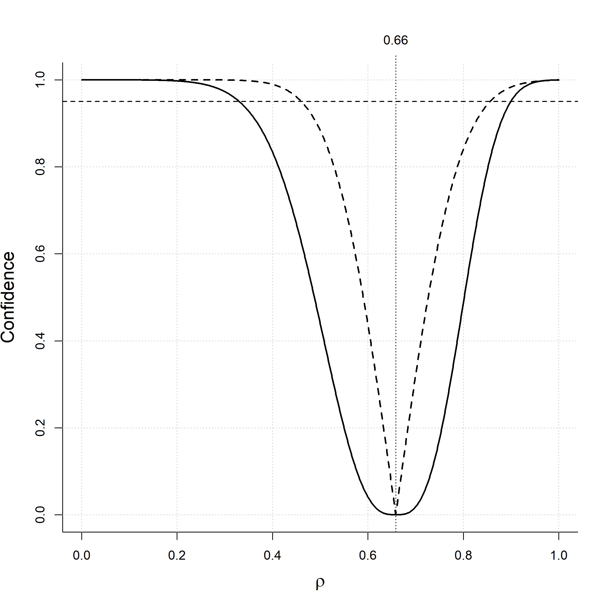
Figure 1: Confidence curves with the $95\%$ confidence set and point estimates emphasized. The solid curves are calculated by the new method and the dashed curve by the Hunter-Schmidt method. . (left) Corrected correlation between Gordon and Piers-Harris from Marx and Winne (1978). (right) Corrected correlation between Facilitation and Agreeableness from Fiori and Antonakis (2012).

2.2 Using Cronbach’s $\alpha$

In the previous section I assumed that $r_{2}$ and $r_{3}$ were sample correlations. But such correlations are hard to come by, since the latent $X,Y$ are almost always unknown. Instead, the reliabilities are estimated indirectly using typically coefficient alpha, which is by far most popular measure of reliability in the psychological literature (McNeish, 2018). Coefficient alpha does not have the same sampling distribution as $r$, so we cannot expect the p-values to be equals. Luckily, it is easy to modify the p-value program 7 to work for coefficient alpha.

The essential ingredient is the formula for the asymptotic distribution of coefficient alpha by van Zyl et al. (2000):

$$n^{1/2}\left[\frac{1}{2}\log\left(1-r^{2}\right)-\frac{1}{2}\log\left(1-\alpha\right)\right]\stackrel{{\scriptstyle d}}{{\to}}N\left(0,\frac{k}{2\left(k-1\right)}\right)$$ (9)

were $\alpha$ is coefficient alpha, $r^{2}$ is its maximum likelihood estimator of $\widehat{\alpha}$, $n$ is the sample size and $k$ is the number of testlets. This result holds under the assumption of multivariate normality and compound symmetry of the covariance matrix of the testlets. Another name for the compound symmetry assumption is that tests are parallell.

The modification of program 8 reads

minimize $$\left(\eta-s\right)^{T}D^{-1}\left(\eta-s\right)$$

subject to $$\rho_{1}\in\left[-1,1\right],R_{i}\in\left[0,1\right],i=2,3$$ (10)

$$\eta_{1}=\text{{artanh}}\left(\rho r_{2}r_{3}\right)$$

where $\eta_{i}=1/2\log\left(1-r_{i}^{2}\right)$ for $i=2,3$ and $D$ is a diagonal matrix with elements $D_{1}=\left(N_{1}-3\right)^{1/2}$, $D_{2}=\left[2N_{2}\left(k_{2}-1\right)/k_{2}\right]^{1/2}$ and $D_{3}=\left[2N_{3}\left(k_{3}-1\right)/k_{3}\right]^{1/2}$, and $r_{2},r_{3}$ are the positive roots of $r_{2}^{2}$ and $r_{3}^{2}$.

3 Coverage of the Confidence Sets

In this section I simulate the coverage of the confidence sets based on correlations (program 7), coefficient alpha (program 10) and the Hunter-Schmidt method 1 using the same setup as Fan (2003). This simulation involves four sample sizes $N$, two different true correlations $\rho$, two different number of testlets $k$, and five different true reliabilities $r^{2}$:

$$N \in \left\{50,100,200,400\right\}$$

$$\rho \in \left\{0.4,0.6\right\}$$

$$k \in \left\{4,8\right\}$$

$$R \in \left\{0.25,0.36,0.49,0.64,0.81\right\}$$

For each combination of $N,\rho,k,R$ I simulate two coefficient alphas $r_{2}^{2},r_{3}^{2}$ based on $k$ testlets, a sample size of $N$, and a true coefficeint alpha of $R$, and one correlation $r=\rho R$ based on a sample size of $N$. I check if the resulting $r,N,k$ are included in the acceptance sets of the three tests at level $\alpha=0.05$. I repeat each simulation $10000$ times. The results can be found in the OSF repository of this paper at https://osf.io/54zea/. I do not show the results for the confidence sets based on correlations since they are not interesting enough. There is no discernible pattern in the coverage, with mean $0.99$ and standard deviation $0.0007$. Figure 2 shows the results of the simulation for the confidence sets based on coefficient alpha and the Hunter-Schmidt method.

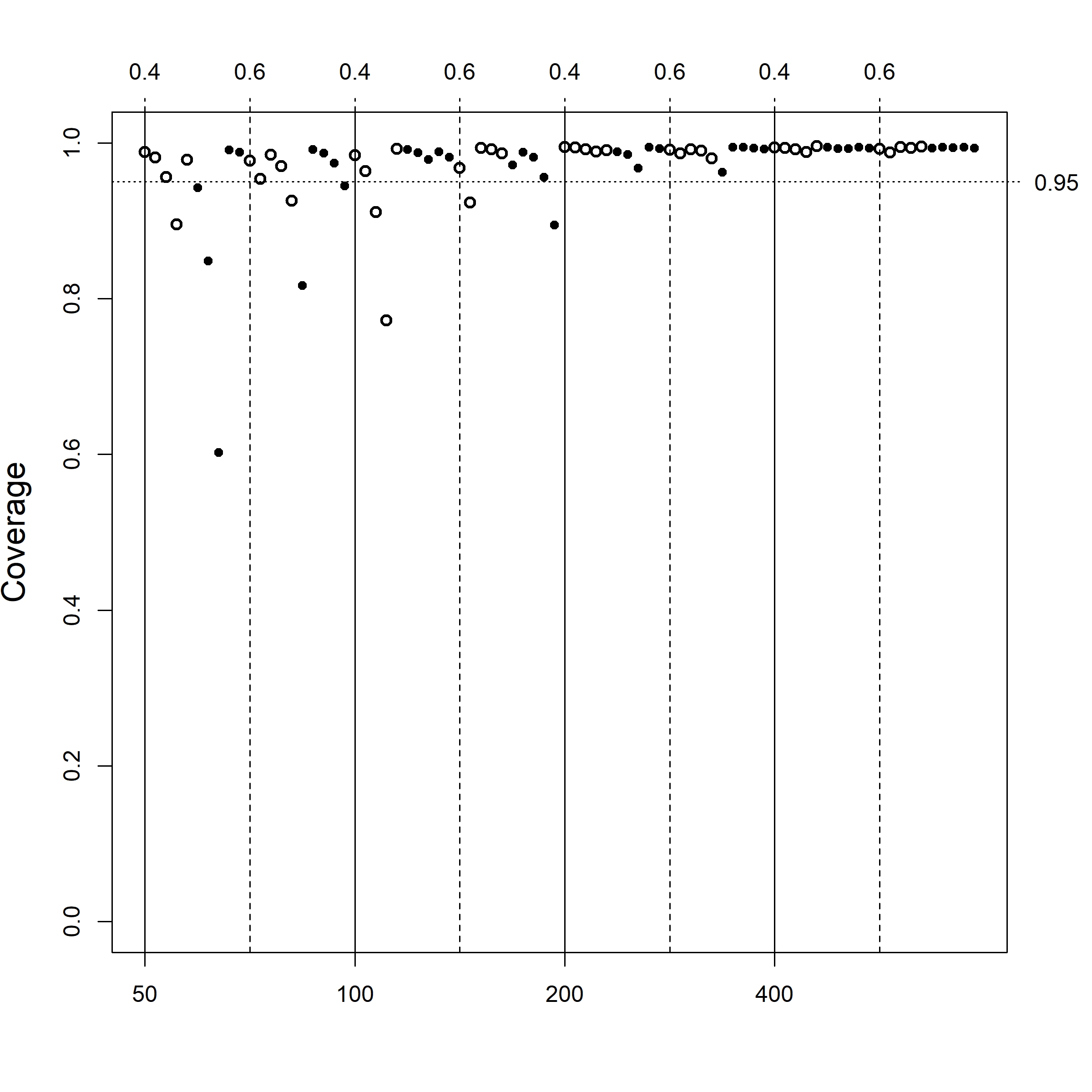
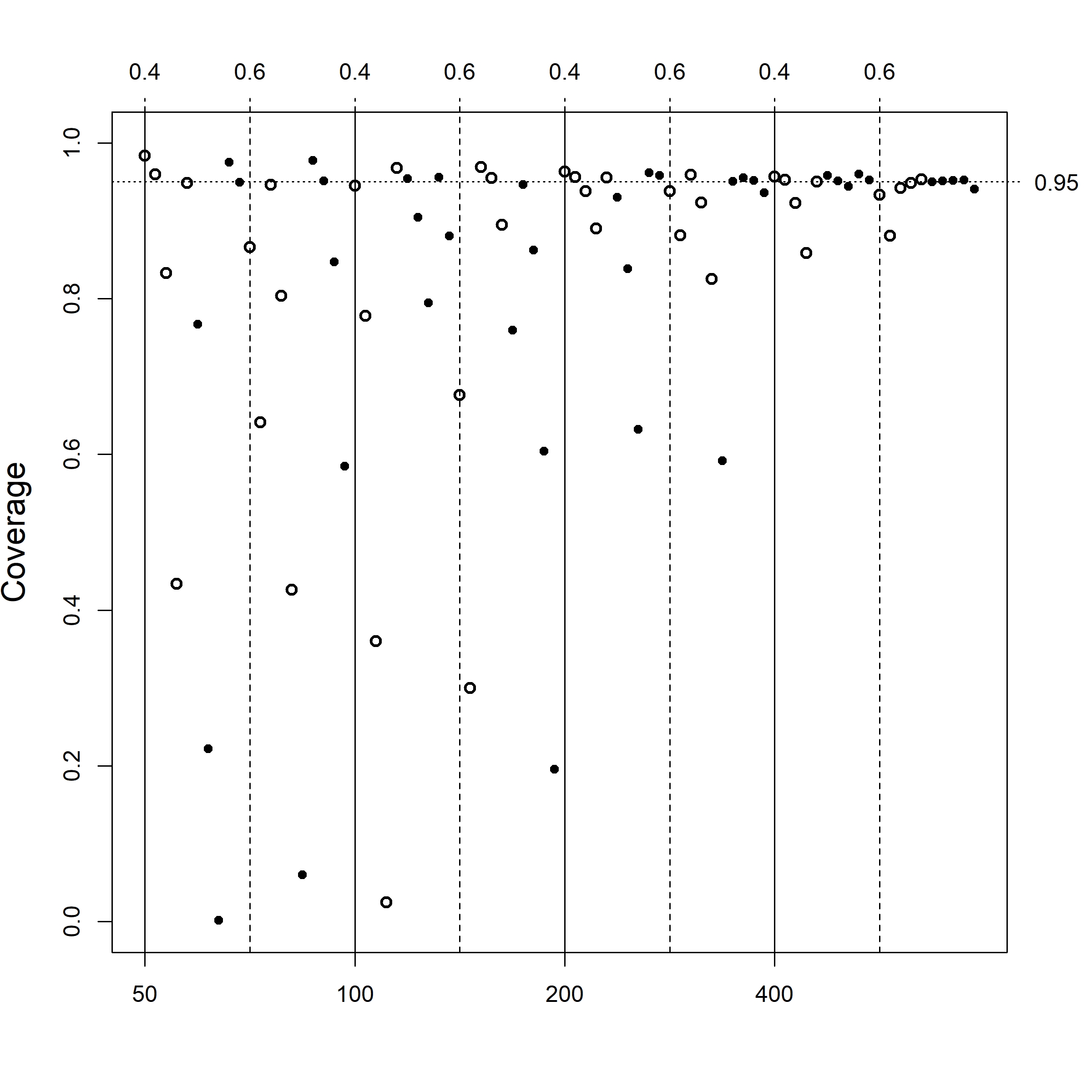
Figure 2: Simulated coverage for the (left) confidence sets based on coefficient alpha (mean: $0.970,$ sd: $0.06$) and (right) the Hunter-Schmidt method (mean: $0.82,$ sd: $0.23$) . The solid vertical lines delineate the different values of $n$ and the dashed vertical lines the different values of $\rho$. The circles correspond to $k=4$, while the solid dots correspond to $k=8$. The rest of the points are ordered according to $r^{2}\in\left\{0.25,0.36,0.49,0.64,0.81\right\}$. The limits on the $y$-axes are not the same in both plots.

The coverage of both the confidence sets based on correlations and the confidence sets based on coefficient alpha are uniformly much larger than the nominal $0.95$.

The confidence sets based on correlations are conservative for all sample sizes, which should be no surprise given their construction. What is more surprising is the poor coverage of the coefficient alpha confidence set for some parameters when the sample size is low. This is probably due to slow convergence of the sample coefficient alpha to the limiting distribution in 9.

The coverage of the confidence sets based on correlations agree well with the confidence sets based on coefficient alpha when the sample size is large. Since the confidence sets based on correlations are easier to calculate, require less information and have better coverage for small sample sizes, it is reasonable to prefer the confidence sets based on correlations. Even if some choices of $N,\rho,k,r^{2}$ turn out to make the coverage of the correlation based confidence set smaller, the conservatism of the confidence set based on correlations is so large the true coverage of the confidence set is likely to be larger than the nominal coverage anyway.

The coverage of the Hunter-Schmidt method is bad for sample sizes smaller than $400$ and horrible when below $200$. On the other hand, its coverage is good for $n=400$. While it fails to achieve a coverage close $0.95$ for all parameter values, it is not nearly as conservative as the new confidence sets.

4 The attenuation package

The R package attenuation has three core functions, p_value for calculating p-values, cc for calculating confidence curves, and ci for calculating confidence sets. Each of these functions support four methods:

• $\mathtt{corr}$: The method based on sample correlation described in program 7.

• $\mathtt{free}$: The method in 7, except that the correlations $\rho_{2},\rho_{3}$ are allowed to be negative.

• $\mathtt{cronbach}$: The method based on the asymptotic distribution for coefficient alpha in 10.

• $\mathtt{HS}$: The Hunter-Schmidt method (1).

The simulations and examples in this paper were done using the attenuation package. It is available on $\mathtt{CRAN}$. Here is an example calculation of a confidence set.

⬇

library("attenuation")

r = c(0.20, sqrt(0.45), sqrt(0.55))

N = c(100, 100, 100)

ci(r, N, method = "corr")

#> [1] -0.1647174 0.9958587

5 Concluding Remarks

My proposed p-value 7 is not likely to be optimal in any sense of the word. Still, it is the result of a reasonable and intuitive construction, and is the first p-value with good behavior under small sample sizes. I note that I have not proven that the p-value has the correct level, as this would require something along the lines of a proof of uniform convergence in distribution (in in $\rho$) of $\left(n-3\right)^{1/2}\left(\textrm{artanh}\left(\rho\right)-\textrm{artanh}\left(r\right)\right)$ to $N\left(0,1\right)$.

The method is conservative, giving confidence sets with true coverage far above the nominal coverage in a simulation that violates its assumption. It would be nice to have smaller confidence sets, perhaps by a modification of the method in this paper. It is well known that the assumptions underlying coefficient alpha as a measure of reliability (i.e tau equivalence) seldom holds (Novick and Lewis, 1967). For instance ”A simulation by Green and Yang (2009a) found that coefficient alpha may underestimate the true reliability by as much as 20% when tau equivalence is violated (e.g., if the true reliability is 0.70, coefficient alpha would estimate reliability in the mid 0.50s).” (McNeish, 2018, p. 4) Since the estimates of the reliability coefficients are likely to be inconsistent, there is a strong extra-statistical case in favor of conservatism.

References

- Benet-Martinez and John (1998) Benet-Martinez, V., John, O.P., 1998. Los cinco grandes across cultures and ethnic groups: Multitrait-multimethod analyses of the big five in spanish and english. Journal of Personality and Social Psychology 75, 729–750.
- Birnbaum (1961) Birnbaum, A., 1961. Confidence curves: An omnibus technique for estimation and testing statistical hypotheses. Journal of the American Statistical Association 56, 246–249.
- Charles (2005) Charles, E.P., 2005. The correction for attenuation due to measurement error: clarifying concepts and creating confidence sets. Psychological Methods 10, 206–226.
- Fan (2003) Fan, X., 2003. Two approaches for correcting correlation attenuation caused by measurement error: Implications for research practice. Educational and Psychological Measurement 63, 915–930.