Global Entanglement Distribution with Multi-mode Non-Gaussian Operations

Abstract

Non-Gaussian operations have been studied intensively in recent years due to their ability to enhance the entanglement of quantum states. However, most previous studies on such operations are carried out in a single-mode setting, even though in reality any quantum state contains multi-mode components in frequency space. Whilst there have been general frameworks developed for multi-mode photon subtraction (PS) and photon addition (PA), an important gap exists in that no framework has thus far been developed for multi-mode photon catalysis (PC). In this work we close that gap. We then apply our newly developed PC framework to the problem of continuous variable (CV) entanglement distribution via quantum-enabled satellites. Due to the high pulse rate envisioned for such systems, multi-mode effects will be to the fore in space-based CV deployments. After determining the entanglement distribution possible via multi-mode PC, we then compare our results with the entanglement distribution possible using multi-mode PS and PA. Our results show that multi-mode PC carried out at the transmitter is the superior non-Gaussian operation when the initial squeezing is below some threshold. When carried out at the receiver, multi-mode PC is found to be the superior non-Gaussian operation when the mean channel attenuation is above some threshold. Our new results should prove valuable for next-generation deployments of CV quantum-enabled satellites.

I Introduction

Non-Gaussian operations are important ingredients for various quantum information tasks, such as quantum teleportation [1], entanglement distillation [2, 3], and quantum error correction [4]. Indeed, in this latter task non-Gaussian effects are a necessary requirement due to the no-go theorem for error correction in a pure Gaussian setting. Having the potential to boost the loss tolerance of quantum states, non-Gaussian operations are also widely studied in the noiseless amplifier [5, 6, 7], and quantum key distribution [8, 9, 10, 11, 12, 13, 14, 15, 16].

At the core of non-Gaussian operations is the application of the ladder operators $\hat{a}$ and $\hat{a}^{\dagger}$ to quantum states, thus altering the photon number statistics. Considering single-mode states, Photon Subtraction (PS), which applies $\hat{a}$ to a state, was first proposed in [17] as a means of producing cat-like states. The operation was then utilized as an efficient way to improve the entanglement of EPR states [18, 19]. The opposite operation, Photon Addition (PA), which applies $\hat{a}^{\dagger}$ to a state, has also been shown to enhance the entanglement of EPR states, at least in a lossless environment [20, 21, 22]. Studies combining PA and PS ($\hat{a}+\hat{a}^{\dagger}$) have also been undertaken e.g., [23, 24, 25, 26]. Such combinations further improve the entanglement but at the price of lower efficiency. Different from PS and PA, Photon Catalysis (PC) applies $\hat{a}^{\dagger}\hat{a}$ to a state. That is, instead of adding or subtracting photons to or from a state, respectively, the PC operation replaces photons from the state. It has been shown previously that PC can enhance entanglement of squeezed EPR states [27, 28]. It can also partially recover the entanglement of states that suffer attenuation [29].

For a given quantum link and initial entangled state, which non-Gaussian operation provides the most entanglement improvement is an interesting question to ask. It turns out that, the best non-Gaussian operation to perform is determined by various settings including, but not limited to, the level of entanglement of the entangled state, the channel conditions, and the locale (transmitter or receiver) where the non-Gaussian operation is performed. Considering all these facts there are two interesting conclusions with regard to the PC operation in the single-mode assumption. At the transmitter, PC provides the most entanglement improvement when the squeezing of the EPR states is below a certain threshold [30]. At the receiver, PC is the best non-Gaussian operation to improve the entanglement when the channel attenuation is above a certain threshold [31].

However, the previous works discussed above are all under the assumption that each beam of the EPR state only contains a single frequency mode. In reality, any quantum state contains multiple frequency modes - an issue of increased concern when broadband pulses of light (narrow pulses in the time domain) are utilized. In such broadband pulses, one frequency mode of the EPR state can be entangled with many other frequency modes. It is therefore natural to investigate whether results derived from single mode analysis are retained for the multi-mode case, or more generally, ask what impact can non-Gaussian operations have on a multiplexed system. To this end, a complete framework of all multi-mode non-Gaussian operations is required. PS and PA in the the multi-mode case have been investigated [32, 33, 34, 35, 36, 37]. However, currently no general framework for multi-mode PC has been established. A key aim of our study is to remedy this situation by developing the full framework for PC in the multi-mode setting. With such a new framework in place we can then fully compare the PS, PA and PC operations in the multi-mode setting. In doing this, we will be particularly interested in the significant potential for entanglement multiplexing gains within such a setting [38, 39, 40].

Our comparison study will be focused on Earth-satellite channels for the quantum entanglement distribution. Recent advances in space-based deployment of quantum communications [41] represent a significant step forward in the creation of global-scale quantum networks. However, it is important to further study quantum communications in this context in the search for improvement in the communications set up, particularly in regard to the global distribution of entanglement - the key resource of any quantum network. Different from [41], in this work we will be considering Continuous Variable (CV) technology embedded in the satellite. For a review of CV quantum communications via satellite see [42].

Our contributions in this work are,

• We develop, for the first time, a general framework for PC in the multi-mode setting.

• We use this new PC multi-mode framework to investigate improvements in entanglement distribution that can be obtained via PC operations applied over Earth-satellite channels.

• We show that the PC operation can be applied to many effective single-mode states (termed ‘supermodes’ in what is to follow) leading to a multiplexed entanglement gain relative to pure single-mode states.

• Finally, we compare the performance of multi-mode PC with multi-mode PS and multi-mode PA in terms of entanglement distribution gains.

The rest of this paper is organized as follows. In Section II we present our framework for the multi-mode PC. In Section III we apply this framework to specific multi-mode entangled states. In Section IV a comparison of multi-mode PS, PA, and PC in terms of entanglement distribution over Earth-satellite channels is provided. Section V concludes our work.

II The General Framework of Photon Catalysis

II-A The Single-mode Case

We begin with a review of the ideal single-mode photon catalysis, which will serve as the cornerstone of the multi-mode case in the next section. Denoting $\hat{a}$ as the annihilation operator of the ancillary state of the photon catalysis operation and $\hat{b}$ the annihilation operator of the state to be catalysed (the input state), as illustrated in Fig. 1a, the single-mode $n$-photon catalysis can be described by an operator $\hat{R}_{n}$. In the Fock basis, this operator has the form

$$\begin{aligned} \hat{R}_{n}&=\bra{n}\hat{U}\left(T\right)\ket{n}\\ &=\bra{0}\frac{\hat{a}^{n}}{\sqrt{n!}}\hat{U}\left(T\right)\frac{\hat{a}^{\dagger n}}{\sqrt{n!}}\ket{0},\end{aligned}$$ (1)

where $\hat{U}\left(T\right)$ is the operator of a Beam Splitter (BS) with transmissivity $T$. Using IWOP (Integration Within an Ordered Product) techniques [43], $\hat{U}\left(T\right)$ can be expressed as [44]

$$\begin{aligned} \hat{U}\left(T\right)=&:\exp\left\{(\sqrt{T}-1)\left(\hat{a}^{\dagger}\hat{a}+\hat{b}^{\dagger}\hat{b}\right)\right.\\ &+\left.\left(\hat{a}^{\dagger}\hat{b}-\hat{a}\hat{b}^{\dagger}\right)\sqrt{\left(1-T\right)}\right\}:,\end{aligned}$$ (2)

where $:\cdot:$ means simple ordering, i.e, ordering the annihilation operators to the right without taking into account the commutation relations. A Fock state has the coherent state representation

$$\ket{n}=\left.\frac{1}{\sqrt{n!}}\frac{\partial^{n}}{\partial\alpha^{n}}\|\alpha\rangle\right|_{\alpha=0},$$ (3)

where $||\alpha\rangle=\exp{(\alpha\hat{a}^{\dagger})\ket{0}}$. Putting Eqs. (2) and (3) into Eq. (1), $\hat{R}_{n}$ can be expressed as [45]

$$\begin{aligned} \hat{R}_{n}=\sqrt{T}^{n}:L_{n}\left(\hat{b}^{\dagger}\hat{b}\frac{1-T}{T}\right):\sqrt{T}^{\hat{b}^{\dagger}\hat{b}},\end{aligned}$$ (4)

where $L_{n}\left(\cdot\right)$ are the Laguerre polynomials. Particularly, when $n=0$ we have the single-mode zero-photon catalysis operator

$$\hat{R}_{0}=\sqrt{T}^{\hat{b}^{\dagger}\hat{b}}.$$ (5)

When $n=1$ we have the single-mode single-photon catalysis operator

$$\hat{R}_{1}=\left(-\frac{1-T}{\sqrt{T}}\hat{b}^{\dagger}\hat{b}+\sqrt{T}\right)\sqrt{T}^{\hat{b}^{\dagger}\hat{b}},$$ (6)

which can also be written as

$$\hat{R}_{1}=\left(-\frac{1-T}{\sqrt{T}}\hat{b}^{\dagger}\hat{b}+\sqrt{T}\right)\hat{R}_{0}.$$ (7)

II-B The Multi-mode Case

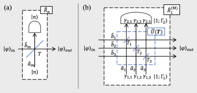
Figure 1: (a) The single-mode $n$-photon catalysis. (b) The multi-mode single-photon catalysis. Here for conciseness only three frequency modes are illustrated.

A multi-mode state is a superposition of single-mode states with different frequency. Let $\hat{a}^{\dagger}_{m}$ be the creation operator of a single-mode state at a specific frequency (indexed with $m$), the creation operator for a multi-mode state is defined as

$$\hat{A}^{\dagger}_{\Gamma_{k}}=\sum_{m=1}^{\infty}\gamma_{k,m}\hat{a}^{\dagger}_{m},$$ (8)

where $\Gamma_{k}=\left[\gamma_{k,1},\gamma_{k,2},...,\gamma_{k,\infty}\right]$ is a normalized complex vector describing the frequency profile of the multi-mode state. The vector $\Gamma_{k}$ is selected from a set of vectors, $\mathbf{\Gamma}=\{\Gamma_{1},\Gamma_{2},...,\Gamma_{\infty}\}$. When the vector elements of $\mathbf{\Gamma}$ are mutually orthogonal, the composed mode created by $\hat{A}^{\dagger}_{\Gamma_{k}}$ is named a supermode.

For the general multi-mode photon catalysis, two major components appearing in the single-mode photon catalysis need to be generalized. These are the Fock state and the BS operator. We first define the multi-mode Fock state as

$$\begin{aligned} \ket{n;\Gamma_{k}}_{A}=\frac{\hat{A}^{\dagger n}_{\Gamma_{k}}}{\sqrt{n!}}&\ket{0},\end{aligned}$$ (9)

which consists of $n$ photons with the same frequency profiles.

We assume that during the multi-mode photon catalysis each single-mode component of the multi-mode state goes through separate independent BSs. In this case, the multi-mode BS is a parallel combination of single-mode BSs. The multi-mode BS operator is defined as

$$\hat{\textbf{U}}\left(\textbf{T}\right)=\bigotimes_{m=1}^{\infty}\hat{U}_{m}\left(T_{m}\right),$$ (10)

where $\hat{U}_{m}\left(T_{m}\right)$ is the single-mode BS operator given by Eq. (2) (acting on a single-mode at the $m$-th frequency), $\textbf{T}=\left\{T_{1},T_{2},...,T_{\infty}\right\}$ is the transmissivity set.

Let $\ket{\varphi}_{\text{in}}$ and $\ket{\varphi}_{\text{out}}$ be the input and output states, the multi-mode $n$-photon catalysis operation can be given by

$$\ket{\varphi}_{\text{out}}=\frac{\hat{R}_{n}^{(\text{M})}}{\sqrt{P}}\ket{\varphi}_{\text{in}},$$ (11)

where $P$ is the success probability for the photon catalysis, and $\hat{R}_{n}^{(\text{M})}$ is the multi-mode $n$-photon catalysis operator. The notation $(\cdot)^{(\text{M})}$ is used to distinguish a multi-mode non-Gaussian operator from its single-mode counterpart. The operator $\hat{R}_{n}^{(\text{M})}$ has a general form

$$\hat{R}_{n}^{(\text{M})}=\left\{\begin{array}[]{cr}\bra{0}\frac{\prod_{k=n+1}^{2n}\hat{A}_{\Gamma_{k}}}{\sqrt{\mathcal{N}_{2}}}\hat{\textbf{U}}\left(\textbf{T}\right)\frac{\prod_{k=1}^{n}\hat{A}_{\Gamma_{k}}^{\dagger}}{\sqrt{\mathcal{N}_{1}}}\ket{0},&n\geq 1\\ \bra{0}\hat{\textbf{U}}\left(\textbf{T}\right)\ket{0},&n=0\end{array}\right.$$ (12)

where $\hat{A}_{\Gamma_{k}}^{\dagger}$’s are multi-mode creation operators defined in Eq. (8), and $\mathcal{N}_{1},\mathcal{N}_{2}\in\left[1,n!\right]$ are normalization constants. It is worth noting that the $n$ photons from the input ancillary Fock state might have different frequency profiles. For the general case, the frequency profiles $\Gamma_{k}$ and $\Gamma_{k^{\prime}}$ are not necessarily orthogonal. The value for $\mathcal{N}_{1}$ is minimized when all the input photons have orthogonal frequency profiles. In this case, the input ancillary state consists of $n$ supermodes. The value for $\mathcal{N}_{1}$ is maximized when the profiles are identical. In this case, the input ancillary state contains only one supermode. Similar to $\mathcal{N}_{1}$, the value of $\mathcal{N}_{2}$ is determined by the frequency profiles of the output detected photons.

III Multi-mode Single-photon Catalysis (MSC)

From the operational point of view, the non-deterministic property of the non-Gaussian operation is an important fact to consider in any implementation [49, 50]. In this regard, the single-photon non-Gaussian operations usually have the highest success probability for a given type of non-Gaussian operation, making them the best candidates for practical implementation. As such, in this work we mainly focus on single-photon non-Gaussian operations. The multi-mode single-photon catalysis (MSC) operation is illustrated in Fig. 1b. The MSC operator can be obtained by setting $n=1$ in Eq. (12),

$$\begin{aligned} \hat{R}_{1}^{(\text{M})}=&\bra{0}\hat{A}_{\Gamma_{2}}\hat{\textbf{U}}\left(\textbf{T}\right)\hat{A}_{\Gamma_{1}}^{\dagger}\ket{0}\\ =&\Bigg{(}\sum_{m,m^{\prime}=1}^{\infty}-\gamma_{1,m}\gamma_{2,m^{\prime}}^{*}\sqrt{1-T_{m}}\sqrt{\frac{1-T_{m^{\prime}}}{T_{m^{\prime}}}}\hat{b}_{m}^{\dagger}\hat{b}_{m^{\prime}}\\ &+\sum_{m=1}^{\infty}\gamma_{1,m}\gamma_{2,m}^{*}\sqrt{T_{m}}\Bigg{)}\bigotimes_{m=1}^{\infty}\sqrt{T_{m}}^{\hat{b}^{\dagger}_{m}\hat{b}_{m}}.\end{aligned}$$ (13)

We are more interested in the case of a frequency non-selective beam splitter ($T_{m}=T$) coupled to an ancillary single-photon state that has frequency profile identical to the output photon ($\Gamma_{1}=\Gamma_{2}=\Gamma_{k}$), which is quite common in experiments [37]. In this work, we will always use this setup when performing the non-Gaussian operations. In this case, the MSC operator $\hat{R}_{1}^{(\text{M})}$ is reduced to

$$\hat{R}_{1}^{(\text{M})}=\left(-\frac{1-T}{\sqrt{T}}\hat{B}^{\dagger}_{\Gamma_{k}}\hat{B}_{\Gamma_{k}}+\sqrt{T}\right)\bigotimes_{m=1}^{\infty}\sqrt{T}^{\hat{b}^{\dagger}_{m}\hat{b}_{m}},$$ (14)

where

$$\hat{B}_{\Gamma_{k}}=\sum_{m=1}^{\infty}\gamma_{k,m}\hat{b}_{m}.$$ (15)

For the special case when $\gamma_{1,m}=\gamma_{2,m}=\delta_{m,1}$, the MSC operator is written

$$\begin{aligned} \hat{R}_{1}^{(\text{M})}=\left(-\frac{1-T_{1}}{\sqrt{T_{1}}}\hat{b}^{\dagger}_{1}\hat{b}_{1}+\sqrt{T_{1}}\right)\sqrt{T_{1}}^{\hat{b}_{1}^{\dagger}\hat{b}_{1}},\end{aligned}$$ (16)

which is simply the single-mode single-photon catalysis operator (on a specific single-mode) given by Eq. (6).

III-A Application of the MSC to a Specific Multi-mode Entangled State

In the single-mode setup, an Einstein-Podolsky-Rosen (EPR) state consists of two entangled single modes. Likewise, in the multi-mode scenario, an EPR state consists of two entangled supermodes. In the following , we label a supermode, $X_{k}$, where $X$ identifies a specific location, and $k$ identifies a specific frequency profile (from a set of orthogonal profiles). For convenience, we introduce another two normalized vectors that characterize the frequency profiles of the two supermodes of the EPR state. Labeling the two supermodes with $B_{k}$ and $D_{k}$, let $\Phi_{k}=\left[\phi_{k,1},\phi_{k,2},...,\phi_{k,\infty}\right]$ and $\Psi_{k}=\left[\psi_{k,1},\psi_{k,2},...,\psi_{k,\infty}\right]$ be the frequency profiles of $B_{k}$ and $D_{k}$, respectively, a multi-mode EPR state is defined as

$$\ket{\text{EPR}_{k}}_{BD}=\sum_{n=0}^{\infty}q_{k,n}\ket{n;\Phi_{k}}_{B}\ket{n;\Psi_{k}}_{D},$$ (17)

where

$$q_{k,n}=\left(\sqrt{1-\tanh^{2}{r_{k}}}\right)\tanh^{n}{r_{k}},$$ (18)

and with $r_{k}$ being the squeezing parameter, and

$$\begin{aligned} \ket{n;\Phi_{k}}_{B}\ket{n;\Psi_{k}}_{D}&=\frac{\hat{B}^{\dagger n}_{\Phi_{k}}}{\sqrt{n!}}\frac{\hat{D}^{\dagger n}_{\Psi_{k}}}{\sqrt{n!}}\ket{0}\\ &:=\ket{n,n;k}_{BD},\end{aligned}$$ (19)

where

$$\hat{B}^{\dagger}_{\Phi_{k}}=\sum_{m=1}^{\infty}\phi_{k,m}\hat{b}^{\dagger}_{m},$$ (20)

and

$$\hat{D}^{\dagger}_{\Psi_{k}}=\sum_{m=1}^{\infty}\psi_{k,m}\hat{d}^{\dagger}_{m},$$ (21)

are the creation operators of the two supermodes.

Suppose we perform the MSC on $B_{k}$, the resultant state reads

$$\begin{aligned} \ket{\psi_{\text{out}}}_{BD}=&\frac{1}{\sqrt{P}}\hat{R}_{1}^{(\text{M})}\ket{\text{EPR}_{k}}_{BD}\\ =&\frac{1}{\sqrt{P}}\left(-\frac{1-T}{\sqrt{T}}\hat{B}^{\dagger}_{\Gamma_{k}}\hat{B}_{\Gamma_{k}}+\sqrt{T}\right)\\ &\times\sum_{n=0}^{\infty}q_{k,n}\sqrt{T}^{n}\ket{n,n;k}_{BD}.\end{aligned}$$ (22)

Suppose the ancillary single-photon state for the MSC are shaped to match the frequency profile of $B_{k}$, i.e., $\Gamma_{k}=\Phi_{k}$. The output state of the MSC operation can then be written

$$\begin{aligned} \ket{\psi_{\text{out}}}_{BD}&=\frac{1}{\sqrt{P}}\sum_{n=0}^{\infty}q_{k,n}\sqrt{T}^{n-1}\left[T-\left(1-T\right)n\right]\ket{n,n;k}_{BD}\\ &:=\frac{1}{\sqrt{P}}\ket{\text{MSC}_{k}}_{BD},\end{aligned}$$ (23)

where $\ket{\text{MSC}_{k}}_{BD}$ is an un-normalized multi-mode photon catalysed EPR state. The success probability for the MSC operation is given by $P=\text{Tr}\{\ket{\text{MSC}_{k}}_{BD}\bra{\text{MSC}_{k}}_{BD}\}$.

III-B Application of the MSC to General Multi-mode Entangled States

More generally, the creation of EPR multi-mode entangled states arise via a Parametric Down-Conversion (PDC) process that leads to simultaneous production of multiple EPR states, each consisting of a pair of entangled supermodes. In this process, a pump laser beam is first fed into a nonlinear crystal. Two correlated beams, labeled signal and idler, are then created. The resultant state can be written in the discrete form as [51]

$$\begin{aligned} \ket{\mathrm{PDC}}_{BD}=\exp\left[i{\hbar}g\left(\sum_{m,m^{\prime}}L_{m,m^{\prime}}\hat{b}^{\dagger}_{m}\hat{d}^{\dagger}_{m^{\prime}}+\mathrm{H.c.}\right)\right]|0\rangle\textrm{,}\end{aligned}$$ (24)

where H.c. represents the Hermitian conjugate, $g$ is the overall gain of the PDC process, $\hat{b}^{\dagger}_{m}$ ($\hat{d}^{\dagger}_{m^{\prime}}$) is the creation operator of the signal (idler) beam at the $m$-th frequency, and $L_{m,m^{\prime}}$ is the Joint Spectrum Amplitude (JSA) function. The PDC process is mainly characterized by the JSA function, which can be decomposed to the following form using the Schmidt decomposition,

$$L_{m,m^{\prime}}=\sum_{k=1}^{\infty}\lambda_{k}\psi_{k,m}\phi_{k,m^{\prime}}\textrm{,}$$ (25)

where $\lambda_{k}$’s are the Schmidt coefficients, and $\psi_{k,m}$ and $\phi_{k,m^{\prime}}$ are entries of the Schmidt basis $\Psi_{k}$ and $\Phi_{k}$, respectively. The PDC state can be viewed as multiple independent multi-mode EPR states using the Schmidt decomposition. Specifically, the PDC state can be re-written as

$$\begin{aligned} \ket{{\mathrm{PDC}}}_{BD}=&\bigotimes_{k=1}^{\infty}\exp\left[r_{k}\hat{B}_{\Phi_{k}}^{\dagger}\hat{D}_{\Psi_{k}}^{\dagger}-\mathrm{H.c.}\right]\ket{0}\\ =&\bigotimes_{k=1}^{\infty}\ket{\text{EPR}_{k}}_{BD},\end{aligned}$$ (26)

where $r_{k}=g\lambda_{k}$, $\hat{B}^{\dagger}_{\Phi_{k}}$and $\hat{D}^{\dagger}_{\Psi_{k}}$ are the supermode creation operators defined in Eqs. (20) and (21), and $\ket{\text{EPR}_{k}}_{BD}$ is a multi-mode EPR state defined in Eq. (17).

Given a collection of multiple EPR states (each consisting of two supermodes) we need to define a detection strategy. The detection strategy we adopt here is one in which the leading supermode (that corresponding to highest eigenvalue) has the MSC operator applied to it, while the remaining supermodes have a zero-photon catalysis operator applied to each of them. This new operator can be written as

$$\begin{aligned} \hat{\textbf{R}}^{(\text{M})}=\hat{R}_{1}^{(\text{M})}\bigotimes_{k=2}^{\infty}\hat{R}_{0}^{(\text{M})},\end{aligned}$$ (27)

where

$$\hat{R}_{0}^{(\text{M})}=\bigotimes_{m=1}^{\infty}\sqrt{T}^{\hat{b}^{\dagger}_{m}\hat{b}_{m}}$$ (28)

is the multi-mode zero-photon catalysis operator.

Applying $\hat{\textbf{R}}^{(\text{M})}$ to the PDC state yields

$$\begin{aligned} \ket{\psi_{\text{out}}}_{BD}=&\frac{1}{\sqrt{P}}\hat{\textbf{R}}^{(\text{M})}\ket{{\mathrm{PDC}}}_{BD}\\ =&\frac{1}{\sqrt{P}}\left[\hat{R}_{1}^{(\text{M})}\ket{\text{EPR}_{1}}_{BD}\bigotimes_{k=2}^{\infty}\hat{R}_{0}^{(\text{M})}\ket{\text{EPR}_{k}}_{BD}\right]\\ =&\frac{1}{\sqrt{P}}\left[\ket{\text{MSC}_{1}}_{BD}\bigotimes_{k=2}^{\infty}\ket{\text{MZC}_{k}}_{BD}\right],\end{aligned}$$ (29)

where

$$\begin{aligned} \ket{\text{MZC}_{k}}_{BD}&=\sum_{n=0}^{\infty}q_{k,n}\underbrace{\sqrt{T}^{\sum_{m=1}^{\infty}\hat{b}_{m}\hat{b}_{m}^{\dagger}}\ket{n;\Phi_{k}}_{B}}_{\sqrt{T}^{n}\ket{n;\Phi_{k}}_{B}}\ket{n;\Psi_{k}}_{D}\\ &=\sum_{n=0}^{\infty}q_{k,n}\sqrt{T}^{n}\ket{n,n;k}_{BD}\end{aligned}$$ (30)

is an un-normalized multi-mode zero-photon catalysed (MZC) state. The success probability $P$ for creation of $\ket{\psi_{\text{out}}}_{BD}$ is written

$$\begin{aligned} P=&\text{Tr}\left\{\left[\ket{\text{MSC}_{1}}_{BD}\bigotimes_{k=2}^{\infty}\ket{\text{MZC}_{k}}_{BD}\right]\times\text{H.c.}\right\}.\\ \end{aligned}$$ (31)

III-C Comparison of Non-Gaussian Operations

For comparison purposes (in the simulations to follow), we also introduce two other multi-mode single-photon non-Gaussian operations, namely the multi-mode single-photon subtraction, and the multi-mode single-photon addition. We also need to define a detection strategy for these new operations. For fairness, we assume the two comparison operations are performed to the PDC state using a detection strategy similar to that adopted for the MSC case. That is, we adopt a strategy in which a multi-mode single-photon subtraction (addition) is applied to the leading supermode, while the remaining supermodes have a zero-photon subtraction (addition) applied to them. Considering that the zero-photon subtraction (and the zero-photon addition) are equivalent to the zero-photon catalysis, the operator for the multi-mode single-photon subtraction can be written

$$\begin{aligned} \hat{\textbf{S}}^{(\text{M})}=\hat{S}_{1}^{(\text{M})}\bigotimes_{k=2}^{\infty}\hat{R}_{0}^{(\text{M})},\end{aligned}$$ (32)

where

$$\hat{S}_{1}^{(\text{M})} =\bra{0}\hat{A}_{\Phi_{1}}\hat{\textbf{U}}\left(\textbf{T}\right)\ket{0}$$ (33)

$$=\sqrt{\frac{1-T}{T}}\hat{B}_{\Phi_{1}}\bigotimes_{m=1}^{\infty}\sqrt{T}^{\hat{b}^{\dagger}_{m}\hat{b}_{m}}.$$ (34)

Likewise, the operator for the multi-mode single-photon addition can be written

$$\begin{aligned} \hat{\textbf{G}}^{(\text{M})}=\hat{G}_{1}^{(\text{M})}\bigotimes_{k=2}^{\infty}\hat{R}_{0}^{(\text{M})},\end{aligned}$$ (35)

where

$$\begin{aligned} \hat{G}_{1}^{(\text{M})}&=\bra{0}\hat{\textbf{U}}\left(\textbf{T}\right)\hat{A}_{\Phi_{1}}^{\dagger}\ket{0}\\ &=-\sqrt{1-T}\hat{B}_{\Phi_{1}}^{\dagger}\bigotimes_{m=1}^{\infty}\sqrt{T}^{\hat{b}^{\dagger}_{m}\hat{b}_{m}}.\end{aligned}$$ (36)

IV Entanglement Distribution over Earth-satellite Channels

In this section we study the entanglement property of the non-Gaussian operations with a concrete example, namely, the evolution of multi-mode states over Earth-satellite channels. In entanglement distribution, Alice (at the transmitter) will send the signal beam of the entangled state to Bob (at the receiver). We will investigate two scenarios as shown in Fig 2. In the first scenario the non-Gaussian operation is performed before the multi-mode state enters the channel. In the second scenario, the non-Gaussian operation is performed after the state has passed through the channel. Three types of non-Gaussian operations, namely the MSC, the multi-mode single-photon subtraction, and the multi-mode single-photon addition will be investigated. We begin this section with a discussion of the Earth-satellite channel model.

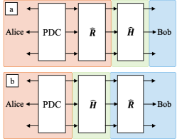
Figure 2: The entanglement distribution with a non-Gaussian operation at the transmitter (a) or at the receiver (b). Here the red, green, and blue boxes illustrate the transmitter, the channel, and the receiver, respectively. The channel is represented by the operator $\hat{H}$ while the non-Gaussian operation is denoted by the operator $\hat{R}$.

IV-A The Earth-satellite Fading Channels

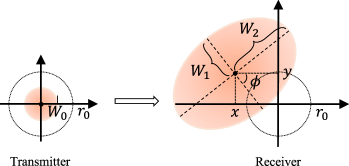
Figure 3: Evolution of the beam-profile over the atmospheric channel. The dotted circle with radius $r_{0}$ illustrates the receiver aperture, and the orange eclipse represents the beam-profile at the receiver.

In atmospheric channels, for optical beams the main loss mechanisms are beam-wandering, beam-broadening, and beam-deformation, all randomly caused by turbulence in the Earth’s atmosphere [52]. The beam-broadening is also a consequence of diffraction. At the receiver, the energy outside the receiver aperture is lost. Over horizontal links the loss mechanisms are well-described by a recent model proposed by [53]. In this model, the profile of the received beam is assumed to have an elliptical shape (see Fig. 3), which is mainly characterized by five real random parameters, namely the 2-D position of the beam-centroid $(x,y)$, the semi-axes of the ellipse $W_{1}$ and $W_{2}$, and the beam rotation angle $\phi$. It is also assumed that $(x,y)$ follows a zero-mean Rayleigh distribution, $W_{1}$ and $W_{2}$ are described by log-normal distributions,, and $\phi$ is uniformly distributed. Let $r_{0}$ be the receiver aperture radius, then the channel transmissivity $\eta$ reads

$$\eta=\eta_{0}\exp\left\{-\left[\frac{\sqrt{x^{2}+y^{2}}/r_{0}}{R(\frac{2}{W_{\rm{eff}}(\phi-\phi_{0})})}\right]^{\lambda\left(2/W_{\rm{eff}}(\phi-\phi_{0})\right)}\right\}\textrm{,}$$ (37)

where $\phi_{0}=\tan^{-1}\frac{y}{x}$,

$$\begin{array}[]{*{20}{l}}W_{\rm{eff}}^{2}(\phi)=&4r_{0}^{2}\left\{\mathcal{W}\left(\frac{4r_{0}^{2}}{W_{1}W_{2}}e^{(r_{0}^{2}/W_{1}^{2})\left[1+2\cos^{2}(\phi)\right]}\right.\right.\\ &\times\left.\left.e^{(r_{0}^{2}/W_{2}^{2})\left[1+2\sin^{2}(\phi)\right]}\right)\right\}^{-1}\end{array}$$ (38)

is the squared effective spot-radius, and

$$\begin{array}[]{*{30}{l}}\eta_{0}=&1-I_{0}\left(r_{0}^{2}\left[\frac{1}{W_{1}^{2}}-\frac{1}{W_{2}^{2}}\right]\right)e^{-r_{0}^{2}\left(1/W_{1}^{2}+1/W_{2}^{2}\right)}\\ &-2\left[1-e^{-(r_{0}^{2}/2)\left[1/W_{1}-1/W_{2}\right]^{2}}\right]\\ &\times\exp\left\{-\left[\frac{\frac{(W_{1}+W_{2})^{2}}{\left|W_{1}^{2}-W_{2}^{2}\right|}}{R\left(\frac{1}{W_{1}}-\frac{1}{W_{2}}\right)}\right]^{\lambda\left(\frac{1}{W_{1}}-\frac{1}{W_{2}}\right)}\right\}\end{array}$$ (39)

is the maximal attainable transmissivity achieved when $(x,y)=(0,0)$ (i.e. no beam-wandering). In the above equations, $\mathcal{W}(\cdot)$ is the Lambert W function, $I_{i}(\cdot)$ is the modified Bessel function of $i$-th order, $R(\xi)$ is a scaling function given by

$$R(\xi)=\left[\ln\left(2\frac{1-\exp\left[-\frac{1}{2}r_{0}^{2}\xi^{2}\right]}{1-\exp\left[-r_{0}^{2}\xi^{2}\right]I_{0}(r_{0}^{2}\xi^{2})}\right)\right]^{-\frac{1}{\lambda(\xi)}}\textrm{,}$$ (40)

and $\lambda(\xi)$ is a shaping function given by

$$\begin{array}[]{*{20}{l}}\lambda(\xi)=&2r_{0}^{2}\xi^{2}\frac{\exp{[-r_{0}^{2}\xi^{2}]}I_{1}(r_{0}^{2}\xi^{2})}{1-\exp\left[-r_{0}^{2}\xi^{2}\right]I_{0}(r_{0}^{2}\xi^{2})}\\ &\times\left[\ln\left(2\frac{1-\exp\left[-\frac{1}{2}r_{0}^{2}\xi^{2}\right]}{1-\exp\left[-r_{0}^{2}\xi^{2}\right]I_{0}(r_{0}^{2}\xi^{2})}\right)\right]^{-1}.\end{array}$$ (41)

In [54] the elliptical model is combined with a scintillation model to characterize the beam evolution over Earth-satellite channels. This requires the introduction of the scintillation index, which can be written [55]

$$\sigma_{I}^{2}=\exp{\left[\frac{0.49\sigma_{R}^{2}}{\left(1+1.11\sigma_{R}^{12/5}\right)^{7/6}}+\frac{0.51\sigma_{R}^{2}}{\left(1+0.69\sigma_{R}^{12/5}\right)^{5/6}}\right]}-1\textrm{,}$$ (42)

where $\sigma_{R}^{2}$ is the Rytov variance given by [52]

$$\sigma_{R}^{2}=2.25k^{7/6}\sec^{11/6}{\zeta}\int_{h_{0}}^{h_{0}+L}C_{n}^{2}\left(h\right)\left(h-h_{0}\right)^{5/6}\,dh,$$ (43)

where $\zeta$ is the zenith angle of the satellite, $h_{0}$ the altitude above sea level of the ground station, and $C_{n}^{2}(h)$ the refractive index structure constant. Using the Hufnagel-Valley model, $C_{n}^{2}(h)$ is described by [56]

$$C_{n}^{2}(h)= 0.00594(v/27)^{2}(h\times 10^{-5})^{10}e^{-\frac{h}{1000}}$$

$$+2.7\times 10^{-16}e^{-\frac{h}{1500}}+Ae^{-\frac{h}{100}}\textrm{,}$$ (44)

where $v$ is the rms wind speed and $A=C_{n}^{2}(0)$.

The mean and variance of $\left\{x,y,\theta_{1},\theta_{2}\right\}$ can be written

$$\begin{aligned} &\left<\theta_{1/2}\right>=\ln{\left[\frac{\left(1+2.96\sigma_{I}^{2}\Omega^{5/6}\right)^{2}}{\Omega^{2}\sqrt{\left(1+2.96\sigma_{I}^{2}\Omega^{5/6}\right)^{2}+1.2\sigma_{I}^{2}\Omega^{5/6}}}\right]},\\ &\left<{\Delta\theta_{1/2}}^{2}\right>=\ln{\left[1+{1.2\sigma_{I}^{2}\Omega^{5/6}}/{\left(1+2.96\sigma_{I}^{2}\Omega^{5/6}\right)^{2}}\right]},\\ &\left<\Delta\theta_{1}\Delta\theta_{2}\right>=\ln{\left[1-{0.8\sigma_{I}^{2}\Omega^{5/6}}/{\left(1+2.96\sigma_{I}^{2}\Omega^{5/6}\right)^{2}}\right]},\\ &\left<\Delta x^{2}\right>=\left<\Delta y^{2}\right>=0.33W_{0}^{2}\sigma_{I}^{2}\Omega^{-7/6},\end{aligned}$$ (45)

where $\theta_{1/2}=\ln\frac{W_{1/2}^{2}}{W_{0}^{2}}$, $W_{0}$ is the initial beam waist, $\Omega=\frac{\pi W_{0}^{2}}{L\lambda}$, $\lambda$ is the beam wavelength, and $L$ is the propagation distance of the transmitted beam.

IV-B Non-Gaussian Operations at the Transmitter

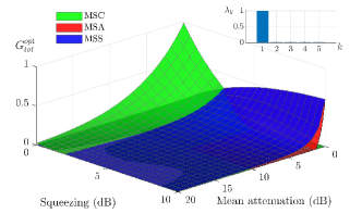
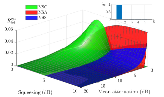
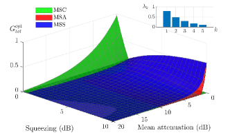
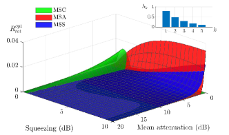
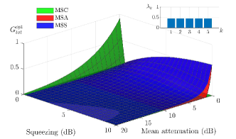
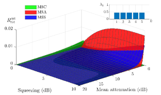
Figure 4: Figures in the the left panel, from top to bottom, illustrate the optimal mean total log-negativity gain $G_{tot}^{opt}$ for the two PDC states. The insets of each figure illustrate the supermode structure of the PDC states. Figures in the right panel illustrate the optimal mean log-negativity gain rate $R_{tot}^{opt}$. Here the multi-mode non-Gaussian operations are performed at the transmitter. (MSC: multi-mode single-photon subtraction, MSA: multi-mode single-photon addition)

Suppose Alice first prepares a PDC state given by Eq. (26). For clarity, we assume that this state only has some finite number $k_{max}$ of supermodes for each beam and Alice only performs the multi-mode non-Gaussian operation on the leading supermode of the signal beam. Considering that the three types of non-Gaussian operations have similar derivations, we use the MSC operation as an example. The resultant state of the MSC operation reads

$$\begin{aligned} \ket{\psi}_{BD}=\frac{1}{\sqrt{P}}\left[\ket{\text{MSC}_{1}}_{BD}\bigotimes_{k=2}^{k_{max}}\ket{\text{MZC}_{k}}_{BD}\right],\end{aligned}$$ (46)

where

$$\begin{aligned} P=&\text{Tr}\left\{\left[\ket{\text{MSC}_{1}}_{BD}\bigotimes_{k=2}^{k_{max}}\ket{\text{MZC}_{k}}_{BD}\right]\times\text{H.c.}\right\}.\\ \end{aligned}$$ (47)

Alice will send the signal beam through the channel, which is modeled by a beam splitter with transmissivity $\eta_{m}$. We also assume that the channel is a pure loss channel, so that the environmental mode can be modeled by a vacuum state. Employing the IWOP techniques the channel for $B_{k}$ can be represented by an operator

$$\begin{aligned} \hat{H}_{k}&=\bigotimes_{m=1}^{\infty}\left[\sqrt{\eta_{m}}^{\hat{b}^{\dagger}_{m}\hat{b}_{m}}\exp\left({\sqrt{1-\eta_{m}}\hat{e}_{m}^{\dagger}\hat{b}_{m}}\right)\right]\ket{0},\\ \end{aligned}$$ (48)

where $\hat{e}_{m}^{\dagger}$ is the creation operator of the environmental mode. For simplicity we assume that the channel is frequency non-selective (i.e., $\eta_{m}=\eta$), the channel operator can be re-written as

$$\begin{aligned} \hat{H}_{k}&=\left[\sqrt{\eta}^{{\hat{B}_{\Phi_{k}}}^{\dagger}\hat{B}_{\Phi_{k}}}\exp\left({\sqrt{1-\eta}\hat{E}_{\Phi_{k}}^{\dagger}\hat{B}_{\Phi_{k}}}\right)\right]\ket{0},\\ \end{aligned}$$ (49)

where $\hat{E}_{\Phi_{k}}^{\dagger}=\sum_{m=1}^{\infty}\phi_{k,m}\hat{e}^{\dagger}_{m}$. Under frequency non-selective assumption the supermodes remain orthogonal after the channel. The entire system, $\ket{\psi}_{DBE}$, after the channel can be written

$$\begin{aligned} \ket{\psi}_{BDE}=&\frac{1}{\sqrt{P}}\left[\hat{H}_{1}\ket{\text{MSC}_{1}}_{BD}\bigotimes_{k=2}^{k_{max}}\hat{H}_{k}\ket{\text{MZC}_{k}}_{BD}\right]\\ =&\frac{1}{\sqrt{P}}\sum_{n=0}^{\infty}\sum_{n^{\prime}=0}^{n}q_{1,n}\sqrt{T}^{n-1}\left[T-\left(1-T\right)n\right]r_{n,n^{\prime}}^{\eta}\\ &\times\ket{n-n^{\prime},n;1}_{BD}\ket{n^{\prime};\Phi_{1}}_{E}\\ &\bigotimes_{k=2}^{k_{max}}\sum_{n=0}^{\infty}\sum_{n^{\prime}=0}^{n}q_{k,n}\sqrt{T}^{n}r_{n,n^{\prime}}^{\eta}\\ &\times\ket{n-n^{\prime},n;k}_{BD}\ket{n^{\prime};\Phi_{k}}_{E},\end{aligned}$$ (50)

where

$$\begin{aligned} r_{n,n^{\prime}}^{\eta}=\sqrt{\left({\begin{array}[]{*{20}{c}}n\\ n^{\prime}\\ \end{array}}\right)}{\sqrt{\eta}^{n-n^{\prime}}}{\sqrt{1-\eta}^{n^{\prime}}}.\end{aligned}$$ (51)

IV-C Non-Gaussian Operations at the Receiver

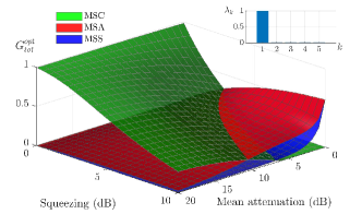
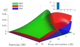
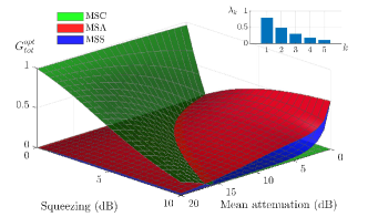
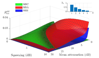
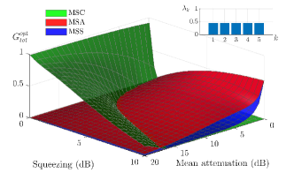
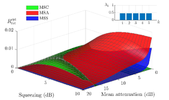
Figure 5: Same as Fig. 4 except that the multi-mode non-Gaussian operations are performed at the receiver. (MSC: multi-mode single-photon subtraction, MSA: multi-mode single-photon addition)

In this section we discuss entanglement distribution with multi-mode non-Gaussian operation performed at the receiver. In this scenario Alice first prepares a PDC state at the transmitter. She then directly sends the signal beam to Bob through the channel while keeping the idler beam. The channel alters the PDC state to the form

$$\begin{aligned} &\ket{\psi}_{BDE}\\ &\quad=\bigotimes_{k=1}^{k_{max}}\hat{H}_{k}\ket{\text{EPR}_{k}}_{BD}\\ &\quad=\bigotimes_{k=1}^{k_{max}}\left[\sum_{n=0}^{\infty}\sum_{{n^{\prime}}=0}^{n}q_{k,n}r_{n,{n^{\prime}}}^{\eta}\ket{n-n^{\prime},n;k}_{BD}\ket{n^{\prime};\Phi_{k}}_{E}\right].\end{aligned}$$ (52)

After receiving the signal beam Bob will perform the MSC on this beam. Similar to the transmitter case, we assume that Bob performs the MSC on the leading supermode of the received signal beam. The resultant state of this operation reads

$$\begin{aligned} &\ket{\psi^{\prime}}_{BDE}\\ &=\frac{1}{\sqrt{P}}\sum_{n=0}^{\infty}\sum_{{n^{\prime}}=0}^{n}q_{1,n}r_{n,{n^{\prime}}}^{\eta}\sqrt{T}^{n-{n^{\prime}}-1}\left[T-\left(1-T\right)\left(n-{n^{\prime}}\right)\right]\\ &\quad\times\ket{n-n^{\prime},n;1}_{BD}\ket{n^{\prime};\Phi_{1}}_{E}\\ &\quad\bigotimes_{k=2}^{k_{max}}\sum_{n=0}^{\infty}\sum_{{n^{\prime}}=0}^{n}q_{k,n}r_{n,{n^{\prime}}}^{\eta}\sqrt{T}^{n-{n^{\prime}}}\\ &\quad\times\ket{n-n^{\prime},n;k}_{BD}\ket{n^{\prime};\Phi_{k}}_{E}\\ &:=\frac{1}{\sqrt{P}}\ket{\psi^{\prime\prime}}_{BDE},\end{aligned}$$ (53)

where the success probability for the MSC operation reads

$$P=\text{Tr}\left(\ket{\psi^{\prime\prime}}_{BDE}\bra{\psi^{\prime\prime}}_{BDE}\right).$$ (54)

IV-D The Measurement of Entanglement

We adopt the log-negativity $E_{LN}$ of the bipartite system as the entanglement measurement. The log-negativity of a state $\rho$ is given by [57]

$$E_{LN}(\rho)=\log_{2}[1+2\varepsilon(\rho)],$$ (55)

where $\varepsilon(\rho)$ is the negativity defined as the absolute value of the sum of the negative eigenvalues of $\rho^{PT}$. We use the total log-negativity gain, which is defined

$$G_{tot}=\text{max}\left[\sum_{k=1}^{k_{max}}\left(E_{LN}(\rho_{k})-E_{LN}(\rho_{k}^{G})\right),\ 0\right],$$ (56)

as our performance metric. Here $\rho_{k}$ is the non-Gaussian state in the $k$-th supermode, and $\rho_{k}^{G}$ is the original Gaussian state on which the non-Gaussian operation is performed. Since the density matrix contains infinite terms, in general the closed form solution to $E_{LN}$ is intractable. Therefore, we approximate $E_{LN}$ by truncating the subsystems $B$, $D$, and $E$ to finite dimensions of $N_{B}$, $N_{D}$, and $N_{E}$, respectively. The density matrix of $B$ and $D$ is obtained by tracing out $E$ in the truncated density matrix. This provides a lower bound to the log-negativity.

In devices which possess quantum memory the success probability, $P$, for the non-Gaussian operations can be neglected. For the situation where the quantum memory is not applicable, we introduce another performance metric, the entanglement gain rate, which reads $R_{tot}=PG_{tot}$.

IV-E Simulation Results

For the Earth-satellite channel, we adopt the parameters from [54]. These are $h_{0}=0$, $v=6\text{m/s}$, and $C_{n}^{2}(0)=9.6\times 10^{-14}\text{m}^{-2/3}$. We focus on vertical down-link channels, which can be easily generalized to non-vertical cases. The initial beam waist and the receiver aperture are set to $W_{0}=6\text{cm}$ and $r_{0}=1\text{m}$, respectively. We note that such a receiver aperture is realistic for ground stations. In accordance with the experiment in [48], the center wavelength of the beam is set as $\lambda=795\text{nm}$ with a bandwidth of roughly $20\text{nm}$. We assume that all the frequency components undergo the same attenuation as the central frequency component. In this case, both the supermode structure and orthogonality of the PDC state after the channel are retained.

A Monte Carlo algorithm is used to simulate the channel since no closed-form solutions to the PDF of the channel transmissivity $\eta$ exists. Let $\eta_{s}$ be the samples generated by the Monte Carlo algorithm, during state transmission, we assume that the channel transmissivity can be measured for each coherent time window, so that the transmissivity $T$ for the beam splitter for the non-Gaussian operations can be adjusted to optimize $G_{tot}$ or $R_{tot}$ for every given $\eta_{s}$. We label the mean optimized $G_{tot}$ and $R_{tot}$ by $G_{tot}^{opt}$ and $R_{tot}^{opt}$, respectively.

Assuming that $k_{max}=5$, we consider three PDC states that have different supermode structures. For the first PDC state, the energy of the supermodes, other than the leading supermode, is assumed close to zero. This state is a good approximation to a single-mode state. The second PDC state is more realistic and contains more than one non-trivial supermodes. For the last PDC state, we assume the 5 supermodes have the same level of squeezing.

We first investigate the scenario where the non-Gaussian operations are performed at the transmitter. In the left panel of Fig. 4, $G_{tot}^{opt}$ is shown as a function of the mean channel attenuation $\bar{\eta}\left[dB\right]=-10\log_{10}\bar{\eta}$ and the squeezing level of the leading supermode $r_{1}\left[dB\right]=-10\log_{10}\left[\exp\left(2{g\lambda_{1}}\right)\right]$, where $g$ is the PDC gain in Eq. (24). We find that the first conclusion mentioned in the introduction is retained for the multi-mode case. That is, at the transmitter the MSC provides larger $G_{tot}^{opt}$ when the initial squeezing is below a threshold. In the multi-mode case this threshold is different from the single-mode case, and is determined by the supermode structure of the state. As such, the parameter settings under which a specific non-Gaussian operation maximizes entanglement is quite different in the single-mode and multi-mode cases. In the right panel of Fig. 4, we compare $R_{tot}^{opt}$ for the three non-Gaussian operations. For the cases where quantum memory is not applicable, MSC is still the best non-Gaussian operation to increase the entanglement when the initial squeezing is below a certain threshold.

We then study the scenario where the non-Gaussian operations are performed at the receiver. Similar to Fig. 4, in the left panel of Fig. 5, $G_{tot}^{opt}$ is illustrated as a function of $\bar{\eta}\left[dB\right]$ and $r_{1}\left[dB\right]$. We find that the second conclusion mentioned in the introduction is also retained. That is, at the receiver, the MSC provides larger $G_{tot}^{opt}$ when $\bar{\eta}$ is above a certain threshold (similar for $R_{tot}^{opt}$ as illustrated in the right panel of Fig. 5). Note that the threshold value is a function of the supermode structure of the state.

V Conclusions

In this work we have established, for the first time, a framework for multi-mode photon catalysis operations. Using our new framework, and focusing on higher success-rate single-photon operations, we then compared photon catalysis operation with photon subtraction and photon addition operations when applied to Earth-satellite channels. Our results show that the outcomes are dependent on whether the operations are carried out at the transmitter or the receiver. In the former case we find that multi-mode photon catalysis is the superior non-Gaussian operation when the initial squeezing is below some threshold. In the latter case we find that multi-mode photon catalysis is the superior non-Gaussian operation when the mean channel attenuation is above some threshold. Our new results will be important for next-generation deployments of quantum-enabled satellites that deploy CV technology. This will be particularly the case when on-board quantum memory becomes available.

References

- [1] T. Opatrnỳ, G. Kurizki, and D.-G. Welsch, “Improvement on teleportation of CV by photon subtraction via conditional measurement,” Physical Review A, vol. 61, no. 3, p. 032302, 2000.
- [2] D. E. Browne, J. Eisert, S. Scheel, and M. B. Plenio, “Driving non-Gaussian to Gaussian states with linear optics,” Physical Review A, vol. 67, no. 6, p. 062320, 2003.
- [3] Y. Kurochkin, A. S. Prasad, and A. Lvovsky, “Distillation of the two-mode squeezed state,” Physical Review Letters, vol. 112, no. 7, p. 070402, 2014.
- [4] J. Niset, J. Fiurášek, and N. J. Cerf, “No-go theorem for Gaussian quantum error correction,” Physical Review Letters, vol. 102, no. 12, p. 120501, 2009.
- [5] J. Jeffers, “Optical amplifier-powered quantum optical amplification,” Physical Review A, vol. 83, no. 5, p. 053818, 2011.
- [6] H.-J. Kim, S.-Y. Lee, S.-W. Ji, and H. Nha, “Quantum linear amplifier enhanced by photon subtraction and addition,” Physical Review A, vol. 85, no. 1, p. 013839, 2012.
- [7] C. Gagatsos, J. Fiurášek, A. Zavatta, M. Bellini, and N. Cerf, “Heralded noiseless amplification and attenuation of non-Gaussian states of light,” Physical Review A, vol. 89, no. 6, p. 062311, 2014.
- [8] P. Huang, G. He, J. Fang, and G. Zeng, “Performance improvement of CV-QKD via photon subtraction,” Physical Review A, vol. 87, no. 1, p. 012317, 2013.
- [9] Z. Li, Y. Zhang, X. Wang, B. Xu, X. Peng, and H. Guo, “Non-Gaussian postselection and virtual photon subtraction in CV-QKD,” Physical Review A, vol. 93, no. 1, p. 012310, 2016.
- [10] Y. Zhao, Y. Zhang, Z. Li, S. Yu, and H. Guo, “Improvement of two-way CV-QKD with virtual photon subtraction,” Quantum Information Processing, vol. 16, no. 8, p. 184, 2017.
- [11] K. Lim, C. Suh, and J.-K. K. Rhee, “CV-QKD protocol with photon subtraction at receiver,” in Proceedings of the International Conference on Quantum Cryptography 2017. QCrypt, 2017.
- [12] Y. Guo, Q. Liao, Y. Wang, D. Huang, P. Huang, and G. Zeng, “Performance improvement of CV-QKD with an entangled source in the middle via photon subtraction,” Physical Review A, vol. 95, no. 3, p. 032304, 2017.
- [13] H.-X. Ma, P. Huang, D.-Y. Bai, S.-Y. Wang, W.-S. Bao, and G.-H. Zeng, “CV MDI-QKD with photon subtraction,” Physical Review A, vol. 97, no. 4, p. 042329, 2018.
- [14] M. He, R. Malaney, and J. Green, “Quantum communications via satellite with photon subtraction,” in IEEE Globecom Workshops. IEEE, 2018, pp. 1–6.
- [15] ——, “Photonic engineering for CV-QKD over Earth-satellite channels,” in IEEE ICC. IEEE, 2019, pp. 1–7.
- [16] W. Ye, H. Zhong, Q. Liao, D. Huang, L. Hu, and Y. Guo, “Improvement of self-referenced CV-QKD with quantum photon catalysis,” Optics Express, vol. 27, no. 12, pp. 17 186–17 198, 2019.
- [17] M. Dakna, T. Anhut, T. Opatrnỳ, L. Knöll, and D.-G. Welsch, “Generating schrödinger-cat-like states by means of conditional measurements on a beam splitter,” Physical Review A, vol. 55, no. 4, p. 3184, 1997.
- [18] P. Cochrane, T. Ralph, and G. Milburn, “Teleportation improvement by conditional measurements on the two-mode squeezed vacuum,” Physical Review A, vol. 65, no. 6, p. 062306, 2002.
- [19] S. Olivares, M. G. Paris, and R. Bonifacio, “Teleportation improvement by inconclusive photon subtraction,” Physical Review A, vol. 67, no. 3, p. 032314, 2003.
- [20] F. Dell’Anno, S. De Siena, L. Albano, and F. Illuminati, “CV quantum teleportation with non-Gaussian resources,” Physical Review A, vol. 76, no. 2, p. 022301, 2007.
- [21] C. Navarrete-Benlloch, R. García-Patrón, J. H. Shapiro, and N. J. Cerf, “Enhancing quantum entanglement by photon addition and subtraction,” Physical Review A, vol. 86, no. 1, p. 012328, 2012.
- [22] S. Zhang, Y. Dong, X. Zou, B. Shi, and G. Guo, “CV-entanglement distillation with photon addition,” Physical Review A, vol. 88, no. 3, p. 032324, 2013.
- [23] V. Parigi, A. Zavatta, M. Kim, and M. Bellini, “Probing quantum commutation rules by addition and subtraction of single photons to/from a light field,” Science, vol. 317, no. 5846, pp. 1890–1893, 2007.
- [24] Y. Yang and F.-L. Li, “Nonclassicality of photon-subtracted and photon-added-then-subtracted Gaussian states,” JOSA B, vol. 26, no. 4, pp. 830–835, 2009.
- [25] S.-Y. Lee, S.-W. Ji, H.-J. Kim, and H. Nha, “Enhancing quantum entanglement for continuous variables by a coherent superposition of photon subtraction and addition,” Physical Review A, vol. 84, no. 1, p. 012302, 2011.
- [26] J. Park, S.-Y. Lee, H.-W. Lee, and H. Nha, “Enhanced Bell violation by a coherent superposition of photon subtraction and addition,” JOSA B, vol. 29, no. 5, pp. 906–911, 2012.
- [27] L. Hu, Z. Liao, and M. S. Zubairy, “CV entanglement via multiphoton catalysis,” Physical Review A, vol. 95, no. 1, p. 012310, 2017.
- [28] Y. Guo, W. Ye, H. Zhong, and Q. Liao, “CV-QKD with non-Gaussian quantum catalysis,” Physical Review A, vol. 99, no. 3, p. 032327, 2019.
- [29] A. E. Ulanov, I. A. Fedorov, A. A. Pushkina, Y. V. Kurochkin, T. C. Ralph, and A. Lvovsky, “Undoing the effect of loss on quantum entanglement,” Nature Photonics, vol. 9, no. 11, p. 764, 2015.
- [30] N. Hosseinidehaj and R. Malaney, “Entanglement generation via non-Gaussian transfer over atmospheric fading channels,” Physical Review A, vol. 92, no. 6, p. 062336, 2015.
- [31] J. Lee and H. Nha, “Entanglement distillation for continuous variables in a thermal environment: Effectiveness of a non-Gaussian operation,” Physical Review A, vol. 87, no. 3, p. 032307, 2013.
- [32] V. A. Averchenko, V. Thiel, and N. Treps, “Nonlinear photon subtraction from a multimode quantum field,” Physical Review A, vol. 89, no. 6, p. 063808, 2014.
- [33] V. Averchenko, C. Jacquard, V. Thiel, C. Fabre, and N. Treps, “Multimode theory of single-photon subtraction,” New Journal of Physics, vol. 18, no. 8, p. 083042, 2016.
- [34] Y.-S. Ra, C. Jacquard, A. Dufour, C. Fabre, and N. Treps, “Tomography of a mode-tunable coherent single-photon subtractor,” Physical Review X, vol. 7, no. 3, p. 031012, 2017.
- [35] M. Walschaers, C. Fabre, V. Parigi, and N. Treps, “Statistical signatures of multimode single-photon-added and-subtracted states of light,” Physical Review A, vol. 96, no. 5, p. 053835, 2017.
- [36] W. N. Plick, F. Arzani, N. Treps, E. Diamanti, and D. Markham, “Violating bell inequalities with entangled optical frequency combs and multipixel homodyne detection,” Physical Review A, vol. 98, no. 6, p. 062101, 2018.
- [37] M. Walschaers, Y.-S. Ra, and N. Treps, “Mode-dependent loss model for multimode photon-subtracted states,” arXiv:1905.06755, 2019.
- [38] A. Christ, C. Lupo, and C. Silberhorn, “Exponentially enhanced quantum communication rate by multiplexing CV teleportation,” New Journal of Physics, vol. 14, no. 8, p. 083007, 2012.
- [39] V. C. Usenko, L. Ruppert, and R. Filip, “Entanglement-based CV-QKD with multimode states and detectors,” Physical Review A, vol. 90, no. 6, p. 062326, 2014.
- [40] N. Hosseinidehaj and R. Malaney, “CV-QKD with Gaussian and non-Gaussian entangled states over satellite-based channels,” in IEEE Global Communications Conference. IEEE, 2016, pp. 1–7.
- [41] S.-K. Liao, W.-Q. Cai, W.-Y. Liu, L. Zhang, Y. Li, J.-G. Ren, J. Yin, Q. Shen, Y. Cao, Z.-P. Li et al., “Satellite-to-ground QKD,” Nature, vol. 549, no. 7670, p. 43, 2017.
- [42] N. Hosseinidehaj, Z. Babar, R. Malaney, S. X. Ng, and L. Hanzo, “Satellite-based continuous-variable quantum communications: state-of-the-art and a predictive outlook,” IEEE Communications Surveys & Tutorials, vol. 21, no. 1, pp. 881–919, 2018.
- [43] H.-y. Fan and L.-y. Hu, “Quantum optical version of classical optical transformations and beyond,” arXiv preprint arXiv:1010.0377, 2010.
- [44] F. Jia, X.-X. Xu, C.-J. Liu, J.-H. Huang, L.-Y. Hu, and H.-Y. Fan, “Decompositions of beam splitter operator and its entanglement function,” Acta Phys. Sin., 2014.
- [45] L.-Y. Hu, J.-N. Wu, Z. Liao, and M. S. Zubairy, “Multiphoton catalysis with coherent state input: nonclassicality and decoherence,” Journal of Physics B: Atomic, Molecular and Optical Physics, vol. 49, no. 17, p. 175504, 2016.
- [46] B. Brecht, A. Eckstein, A. Christ, H. Suche, and C. Silberhorn, “From quantum pulse gate to quantum pulse shaper—engineered frequency conversion in nonlinear optical waveguides,” New Journal of Physics, vol. 13, no. 6, p. 065029, 2011.
- [47] S. Armstrong, J.-F. Morizur, J. Janousek, B. Hage, N. Treps, P. K. Lam, and H.-A. Bachor, “Programmable multimode quantum networks,” Nature Communications, vol. 3, p. 1026, 2012.
- [48] J. Roslund, R. M. De Araujo, S. Jiang, C. Fabre, and N. Treps, “Wavelength-multiplexed quantum networks with ultrafast frequency combs,” Nature Photonics, vol. 8, no. 2, p. 109, 2014.
- [49] T. J. Bartley, P. J. Crowley, A. Datta, J. Nunn, L. Zhang, and I. Walmsley, “Strategies for enhancing quantum entanglement by local photon subtraction,” Physical Review A, vol. 87, no. 2, p. 022313, 2013.
- [50] T. J. Bartley and I. A. Walmsley, “Directly comparing entanglement-enhancing non-Gaussian operations,” New Journal of Physics, vol. 17, no. 2, p. 023038, 2015.
- [51] R. M. de Araújo, J. Roslund, Y. Cai, G. Ferrini, C. Fabre, and N. Treps, “Full characterization of a highly multimode entangled state embedded in an optical frequency comb using pulse shaping,” Physical Review A, vol. 89, no. 5, p. 053828, 2014.
- [52] L. C. Andrews and R. L. Phillips, Laser beam propagation through random media. SPIE press Bellingham, WA, 2005, vol. 152.
- [53] D. Vasylyev, A. Semenov, and W. Vogel, “Atmospheric quantum channels with weak and strong turbulence,” Physical Review Letters, vol. 117, no. 9, p. 090501, 2016.
- [54] Y. e. a. Guo, “Channel-parameter estimation for satellite-to-submarine CV-QKD,” Physical Review A, vol. 97, no. 5, p. 052326, 2018.
- [55] L. C. Andrews, R. L. Phillips, and C. Y. Young, “Scintillation model for a satellite communication link at large zenith angles,” Optical Engineering, vol. 39, no. 12, pp. 3272–3281, 2000.
- [56] R. R. Beland, “Propagation through atmospheric optical turbulence,” Atmospheric Propagation of Radiation, vol. 2, pp. 157–232, 1993.
- [57] G. Vidal and R. F. Werner, “Computable measure of entanglement,” Physical Review A, vol. 65, no. 3, 2002.