The generalization error of max-margin linear classifiers:
Benign overfitting and high dimensional asymptotics in the overparametrized regime

Abstract

Modern machine learning classifiers often exhibit vanishing classification error on the training set. They achieve this by learning nonlinear representations of the inputs that maps the data into linearly separable classes.

Motivated by these phenomena, we revisit high-dimensional maximum margin classification for linearly separable data. We consider a stylized setting in which data $(y_{i},{\boldsymbol{x}}_{i})$, $i\leq n$ are i.i.d. with ${\boldsymbol{x}}_{i}\sim\mathsf{N}({\boldsymbol{0}},{\boldsymbol{\Sigma}})$ a $p$-dimensional Gaussian feature vector, and $y_{i}\in\{+1,-1\}$ a label whose distribution depends on a linear combination of the covariates $\langle{\boldsymbol{\theta}}_{*},{\boldsymbol{x}}_{i}\rangle$. While the Gaussian model might appear extremely simplistic, universality arguments can be used to show that the results derived in this setting also apply to the output of certain nonlinear featurization maps.

We consider the proportional asymptotics $n,p\to\infty$ with $p/n\to\psi$, and derive exact expressions for the limiting generalization error. We use this theory to derive two results of independent interest: $(i)$ Sufficient conditions on $({\boldsymbol{\Sigma}},{\boldsymbol{\theta}}_{*})$ for ‘benign overfitting’ that parallel previously derived conditions in the case of linear regression; $(ii)$ An asymptotically exact expression for the generalization error when max-margin classification is used in conjunction with feature vectors produced by random one-layer neural networks.

1 Introduction

1.1 Background

Modern machine learning models for classification, such as multi-layer neural networks, are a composition of multiple nonlinear maps, which produce increasingly simple representations of the data. A linear readout unit outputs the class label. In the case of binary classification, on input ${\boldsymbol{z}}\in\mathbb{R}^{d}$, such a model outputs

$$\hat{y}({\boldsymbol{z}})=\mathop{\rm sign}\,\langle{\boldsymbol{\theta}},{\boldsymbol{\phi}}({\boldsymbol{z}};{\boldsymbol{W}})\rangle\,,$$ (1.1)

where the featurization map ${\boldsymbol{\phi}}:\mathbb{R}^{d}\to\mathbb{R}^{p}$ encodes a nonlinear data representation, parametrized by weights ${\boldsymbol{W}}$. For instance, in the case of a multi-layer neural network, ${\boldsymbol{\phi}}({\boldsymbol{z}};{\boldsymbol{W}})=\sigma\circ{\boldsymbol{W}}_{1}\circ\sigma\circ\cdots\sigma\circ{\boldsymbol{W}}_{L}{\boldsymbol{z}}$.

In the practice of machine learning, it is often the case that these models achieve vanishing error on the training data and, despite this, they generalize well to unseen data. Vanishing training error means that the representation ${\boldsymbol{\phi}}({\boldsymbol{z}};{\boldsymbol{W}})$ is able to map the data into linearly separable classes. There are two possible mechanisms for this:

• The parameters ${\boldsymbol{W}}$ are also learnt from training data, and hence ${\boldsymbol{\phi}}(\;\cdot\;;{\boldsymbol{W}})$ is a highly non-linear data-dependent map that makes the data separable. Notice that by allowing for a sufficiently rich class of maps ${\boldsymbol{\phi}}(\;\cdot\;;{\boldsymbol{W}})$, linear separability can be achieved even with a low embedding dimension $p$.

• The map ${\boldsymbol{\phi}}(\;\cdot\;;{\boldsymbol{W}})$ is not learnt from the same training data and it is possibly entirely random. In this case, linear separability emerges mainly because of the dimension blow up from $d$ to $p$.

While both mechanisms —learning and dimensionality blow-up— are relevant for fully trained neural networks, this paper focuses on the second aspect. This is most important for nonlinear models in the neural tangent or lazy regime [JGH18], but also for kernel methods [HSS08, Wah02] and for their random features approximation [Nea96, BBV06, RR08]. Notice that in these applications, the interpretation of the features dimensions $p$ varies. For instance, in the case of neural nets in the lazy regime, $p$ is the overall number of parameter, and not just the size of the last layer. Given the current status of mathematical technology, the dimensionality blow-up is more amenable to rigorous analysis and yet very challenging. Indeed, we will leave several mathematical questions unsolved and, despite the substantial follow-up work, many questions have been unsolved since the first appearance of this manuscript.

We are thus led to consider the set of linear classifiers with vanishing empirical error, namely:

$${\rm ERM}_{0}({\boldsymbol{y}},{\boldsymbol{X}}) :=\Big{\{}{\boldsymbol{\theta}}\in\mathbb{R}^{p}:\,\,\|{\boldsymbol{\theta}}\|_{2}=1,\;\;\min_{i\leq n}y_{i}\langle{\boldsymbol{\theta}},{\boldsymbol{x}}_{i}\rangle\geq 0\;\Big{\}}\,,$$ (1.2)

$${\boldsymbol{X}} =\left[\begin{matrix}\;\text{---}\;{\boldsymbol{x}}_{1}\;\text{---}\;\\ \vdots\\ \;\text{---}\;{\boldsymbol{x}}_{n}\;\text{---}\;\end{matrix}\right]\,,\;\;\;\;{\boldsymbol{x}}_{i}={\boldsymbol{\phi}}({\boldsymbol{x}}_{i};{\boldsymbol{W}})\,,$$ (1.3)

where ${\boldsymbol{\phi}}(\,\cdot\,;{\boldsymbol{W}})$ is a featurization map independent of the data.

A rich line of work supports the intuition that among all the possible classifiers with vanishing training error ${\boldsymbol{\theta}}\in{\rm ERM}_{0}({\boldsymbol{y}},{\boldsymbol{X}})$, the ones selected by optimization algorithms used in practice have special ‘simplicity’ properties [SHN⁺18, GLSS18b, LMZ17, GLSS18a, ACHL19]. This phenomenon is commonly referred to as ‘implicit regularization.’

Of particular interest (and our focus in this paper) is the max-margin classifier:

$$\hat{\boldsymbol{\theta}}^{\mbox{\tiny\rm MM}}({\boldsymbol{y}},{\boldsymbol{X}}):=\arg\max\Big{\{}\;\;\min_{i\leq n}y_{i}\langle{\boldsymbol{\theta}},{\boldsymbol{x}}_{i}\rangle:\;\;\;\|{\boldsymbol{\theta}}\|_{2}=1\;\;\Big{\}}\,.$$ (1.4)

Indeed, it was proven in [SHN⁺18] that gradient descent (with respect to logistic loss) converges to $\hat{\boldsymbol{\theta}}^{\mbox{\tiny\rm MM}}({\boldsymbol{y}},{\boldsymbol{X}})$. Namely, considering the gradient-descent iteration

$$\hat{\boldsymbol{\theta}}^{k+1}=\hat{\boldsymbol{\theta}}^{k}-s_{k}\nabla\hat{L}_{n}(\hat{\boldsymbol{\theta}}^{k})\,,\;\;\;\hat{L}_{n}({\boldsymbol{\theta}})\equiv\frac{1}{n}\sum_{i=1}^{n}\left\{-y_{i}\langle{\boldsymbol{\theta}},{\boldsymbol{x}}_{i}\rangle+\log\big{(}e^{\langle{\boldsymbol{\theta}},{\boldsymbol{x}}_{i}\rangle}+e^{-\langle{\boldsymbol{\theta}},{\boldsymbol{x}}_{i}\rangle}\big{)}\right\}\,.$$ (1.5)

we have $\hat{\boldsymbol{\theta}}^{k}/\|\hat{\boldsymbol{\theta}}^{k}\|\to\hat{\boldsymbol{\theta}}^{\mbox{\tiny\rm MM}}$ as $k\to\infty$.

In this paper, we will study the generalization error of max-margin classification for i.i.d. separale data $(y_{i},{\boldsymbol{x}}_{i})$, $i\leq n$. For this purpose, the form of the featurization map ${\boldsymbol{z}}_{i}\mapsto{\boldsymbol{x}}_{i}={\boldsymbol{\phi}}({\boldsymbol{z}}_{i};{\boldsymbol{W}})$ only matters to the extent that it determines the distribution of the feature vectors ${\boldsymbol{x}}_{i}$ given the underlying distribution of the ${\boldsymbol{z}}_{i}$. We will consider a stylized model whereby the features are Gaussian with population covariance ${\boldsymbol{\Sigma}}$: ${\boldsymbol{x}}_{i}\sim\mathsf{N}(0,{\boldsymbol{\Sigma}})$. At first sight, this might appear to be unrelated to the original problem. However, as further discussed below, recent universality results [HL22, MS22], as well as our companion paper [MR⁺23], indicate that the characterization we obtain for Gaussian features applies to a class of featurization maps provided we match the covariances ${\boldsymbol{\Sigma}}=\mathbb{E}_{{\boldsymbol{z}}}[{\boldsymbol{\phi}}({\boldsymbol{z}};{\boldsymbol{W}}){\boldsymbol{\phi}}({\boldsymbol{z}};{\boldsymbol{W}})^{{\sf T}}]$.

Throughout this paper we will say that a model is overparametrized if the set of zero-error classifiers ${\rm ERM}_{0}({\boldsymbol{y}},{\boldsymbol{X}})$ is non-empty. Over the last couple of years, the generalization properties of overparametrized models have attracted considerable interest (see also Section 4). A unified phenomenology has emerged from simulation studies with a number of statistical models, including kernel methods, random forests, and multilayer neural networks [BHMM19]

In order to discuss this phenomenology, it is convenient to regard the prediction error as a function of two quantities: the sample size $n$ and the number of parameters $p$. The classical statistical theory assumes that $p$ is fixed and is related to the data distribution. $p$ can be either smaller or larger than $n$ depending on whether the low-dimensional or high-dimensional regimes are considered, but typically larger $p$ is regarded as yielding a different, ‘harder’, data distribution. In contrast, we think here of the data distribution as fixed, and larger $p$ corresponds to different featurization maps. When looking at the possibility of increasing $p$ in this way, two interesting statistical behaviors have been observed repeatedly:

1. Benign overfitting. The excess error (difference between the prediction error and the Bayes error) can vanish as $p,n$ get large, despite: $(i)$ the model is extremely overparametrized $p\gg n$; $(ii)$ the model is not regularized and in particular, it has vanishing training error.

2. Optimality of overfitting. For certain data distributions, the test error of overparametrized models is smaller than the test error of underparametrized ones. In particular, the test error is minimized when $p/n\gg 1$.

Rigorous confirmation of these phenomena were established in a number of papers [BHX19, BHM18, HMRT22, BLLT20, TB20, MM19, MZ22]. (See Section 4 for further references.) The bulk of these rigorous studies, and by far the most detailed picture was developed in the case of ridge regression and its ridge-less limit min-norm regression. A number of models for the feature vectors ${\boldsymbol{x}}_{i}$ were studied in this context: unstructured distributions with prescribed covariance [HMRT22, BLLT20], kernel methods [LR20] random features models [MM22], and neural tangent features [MZ22]. However, all of these works rely on the linear-algebraic structure of the ridge estimator, and leverage tools from random matrix theory to characterize its behavior. Moving beyond ridge regression is an important step that requires fundamentally different mathematical ideas.

At this point, it is legitimate to wonder whether max-margin classification warrants being revisited. After all, the machine learning community has devoted significant attention to the analysis of max-margin classifiers. An incomplete selection of references include [Bar98, AB09, KP02, BM02, KST09, Kol11]. This line of work develops upper bounds on the generalization error (difference between test and training error) in terms of the complexity (e.g. the Radamacher complexity) of the underlying function class. In the case of maximum margin classification, this approach yields upper bounds that depend on the empirical margin or the empirical margin distribution. In this theory, the empirical margin concentrates around the population margin (or the population margin distribution). Intuitively, data are (approximately) separable because the signal-to-noise ratio is very strong.

In contrast, we are interested in cases in which the signal-to-noise ratio is moderate and the population distribution is not linearly separable (not even approximately so). In the regime studied here, separability is a high-dimensional phenomenon that arises because of overparametrization. Appendix L illustrates this claim by providing concrete examples in which classical margin-based bounds fail to capture the qualitative behavior of the generalization error.

1.2 Overview of results

We assume the feature vectors ${\boldsymbol{x}}_{i}$ to be independent draws from a $p$-dimensional centered Gaussian with covariance ${\boldsymbol{\Sigma}}$, and responses to be distributed according to

$$\mathbb{P}\big{(}y_{i}=+1\big{|}{\boldsymbol{x}}_{i}\big{)} =1-\mathbb{P}\big{(}y_{i}=-1\big{|}{\boldsymbol{x}}_{i}\big{)}=f(\langle{\boldsymbol{\theta}}_{*},{\boldsymbol{x}}_{i}\rangle)\,,$$ (1.6)

$${\boldsymbol{x}}_{i} \sim\mathsf{N}({\boldsymbol{0}},{\boldsymbol{\Sigma}})\,.$$ (1.7)

We will assume throughout the proportional asymptotics

$$n,p\to\infty\quad\textnormal{with}\quad\frac{p}{n}\to\psi\in(0,\infty),$$ (1.8)

and determine the precise asymptotics of the test error. In what follows, we will index sequence of instances by $n\in\mathbb{N}$, and it will be understood that $p=p_{n}$.

In order for the limit to exist and be well defined, we need to make certain assumptions about the behavior of the covariance matrix ${\boldsymbol{\Sigma}}={\boldsymbol{\Sigma}}_{n}$ and the ‘true’ parameters vector ${\boldsymbol{\theta}}_{*}={\boldsymbol{\theta}}_{*,n}$. These are -in a way– analogous to the assumptions made in random matrix theory to derive the asymptotics of the empirical spectral distribution.

Let ${\boldsymbol{\Sigma}}_{n}=\sum_{i=1}^{p}\lambda_{i}{\boldsymbol{v}}_{i}{\boldsymbol{v}}_{i}^{{\sf T}}$ be the eigenvalue decomposition of ${\boldsymbol{\Sigma}}$, with $\lambda_{1}\geq\lambda_{2}\geq\dots\geq\lambda_{p}$. Our first assumption requires that the eigenvalues of ${\boldsymbol{\Sigma}}$ do not decay too rapidly.

Assumption 1.

Denote $\lambda_{\max}({\boldsymbol{\Sigma}}_{n})=\lambda_{1}({\boldsymbol{\Sigma}}_{n})$. There exist constants $\lambda_{\textsf{M}},L>0,$ and $\varepsilon>0$ such that

$$\lambda_{\max}({\boldsymbol{\Sigma}}_{n})\leq\lambda_{\textsf{M}}\,,$$ (1.9)

and

$$\frac{1}{p}\sum_{i=1}^{p}\left(\frac{1}{\lambda_{i}({\boldsymbol{\Sigma}}_{n})}\right)^{1+\varepsilon}\leq L.$$

Our second assumption concerns the eigenvalue distribution of ${\boldsymbol{\Sigma}}_{n}$ as well as the decomposition of ${\boldsymbol{\theta}}_{*,n}$ in the basis of eigenvectors of ${\boldsymbol{\Sigma}}_{n}$.

Assumption 2.

Let $\rho_{n}\equiv\langle{\boldsymbol{\theta}}_{*,n},{\boldsymbol{\Sigma}}_{n}{\boldsymbol{\theta}}_{*,n}\rangle^{1/2}$ and $\bar{w}_{i}\equiv\sqrt{p\lambda_{i}}\langle{\boldsymbol{v}}_{i},{\boldsymbol{\theta}}_{*,n}\rangle/\rho_{n}$. Then the empirical distribution of $\{(\lambda_{i},\bar{w}_{i})\}_{1\leq i\leq n}$ converges in Wasserstein-$2$ distance to a probability distribution $\mu$ on $\mathbb{R}_{>0}\times\mathbb{R}$:

$$\frac{1}{p}\sum_{i=1}^{p}\delta_{(\lambda_{i},\bar{w}_{i})}\stackrel{{\scriptstyle W_{2}}}{{\Longrightarrow}}\mu\,.$$ (1.10)

In particular, $\int w^{2}\mu({\rm d}\lambda,{\rm d}w)=1$, and we have that

$$\rho\equiv\lim_{n\to\infty}\rho_{n}=\int(w^{2}/\lambda)\mu({\rm d}\lambda,{\rm d}w).$$ (1.11)

We refer the reader to Appendix A for a reminder of the definition of the Wasserstein distance $W_{2}$. Here, we limit ourselves to mentioning that convergence in $W_{2}$ is equivalent to weak convergence plus the convergence of the second moment, see e.g. [Vil08]. In particular, the condition $\int(w^{2}/\lambda)\mu({\rm d}\lambda,{\rm d}w)=1/\rho^{2}$ implies $\lim_{n\to\infty}\|{\boldsymbol{\theta}}_{*,n}\|_{2}=1$. Notice that this choice of normalization implies no loss of generality: if $\lim_{n\to\infty}\|{\boldsymbol{\theta}}_{*,n}\|_{2}=c\neq 1$, we can rescale ${\boldsymbol{\theta}}_{*,n}$ (letting ${\boldsymbol{\theta}}^{\mbox{\tiny\rm new}}_{*,n}={\boldsymbol{\theta}}_{*,n}/c$) and the function $f$ (letting $f^{\mbox{\tiny\rm new}}(t)=f(ct)$), as to satisfy the assumed normalization.

Finally, we state our assumptions on the function $f$.

Assumption 3.

Define $T=YG$ where

$$\mathbb{P}(Y=1\mid G)=1-\mathbb{P}(Y=-1\mid G)=f(\rho\cdot G),\quad G\sim\mathsf{N}(0,1).$$ (1.12)

We assume $f:\mathbb{R}\to[0,1]$ to be continuous, and it satisfies the following non-degeneracy condition:

$$\inf\Big{\{}x:\mathbb{P}(T<x)>0\Big{\}}=-\infty\leavevmode\nobreak\ \leavevmode\nobreak\ \text{and}\leavevmode\nobreak\ \leavevmode\nobreak\ \sup\Big{\{}x:\mathbb{P}(T>x)>0\Big{\}}=\infty\,.$$

It is easy to check that the non-degeneracy condition is satisfied for most ‘reasonable’ choices of $f$. In particular, it is sufficient that $f(x)\in(0,1)$ for all $x$.

Remark 1.1.

At first sight, Assumption 2 is the strongest of our conditions. Note however that the convergence of Eq. (1.10) always holds along subsequences under some tightness condition (by Prokhorov’s theorem). For instance, this is the case if we assume that $\sum_{i=1}^{p}|\lambda_{i}|^{2+\varepsilon}\leq C\,p$ and $\sum_{i=1}^{p}|\bar{w}_{i}|^{2+\varepsilon}\leq C\,p$ hold for some constants $C,\varepsilon>0$.

Under tightness, we could always apply our theory to characterize each converging subsequence of instances.

Under these assumptions, we establish the following results.

Asymptotic characterization of the maximum margin.

Define the maximum margin by

$$\kappa_{n}({\boldsymbol{y}},{\boldsymbol{X}})\equiv\max\big{\{}\min_{i\leq n}y_{i}\langle{\boldsymbol{\theta}},{\boldsymbol{x}}_{i}\rangle:\;\;{\boldsymbol{\theta}}\in\mathbb{R}^{p},\;\|{\boldsymbol{\theta}}\|_{2}=1\big{\}}\,.$$ (1.13)

We prove that $\kappa_{n}({\boldsymbol{y}},{\boldsymbol{X}})\to\kappa^{*}(\mu,\psi)$ in probability as $n\to\infty$ for some non-random asymptotic margin $\kappa^{*}(\mu,\psi)$. We give an explicit characterization of the limiting value $\kappa^{*}(\mu,\psi)$, stated in Section 5.

As a corollary, we derive the limiting value of the interpolation threshold, i.e. the minimum number of parameters per dimensions above which the data are linearly separable with a positive margin: $\psi^{*}(\mu)\equiv\inf\{\psi\geq 0:\;\kappa^{*}(\mu,\psi)>0\}$, and below which the data are non-separable. (This generalizes the recent result of [CS18].)

Asymptotic characterization of prediction error.

Let the test error be defined by

$${\rm Err}_{n}({\boldsymbol{y}},{\boldsymbol{X}})\equiv\mathbb{P}\big{(}y^{\mbox{\tiny\rm new}}\langle\hat{\boldsymbol{\theta}}^{\mbox{\tiny\rm MM}}({\boldsymbol{y}},{\boldsymbol{X}}),{\boldsymbol{x}}^{\mbox{\tiny\rm new}}\rangle\leq 0\big{)}\,,$$ (1.14)

where expectation is with respect to a fresh sample $(y^{\mbox{\tiny\rm new}},{\boldsymbol{x}}^{\mbox{\tiny\rm new}})$ independent of the data $({\boldsymbol{y}},{\boldsymbol{X}})$. We will sometimes refer to ${\rm Err}_{n}({\boldsymbol{y}},{\boldsymbol{X}})$ as to the prediction error. We prove that ${\rm Err}_{n}({\boldsymbol{y}},{\boldsymbol{X}})\to{\rm Err}^{*}(\mu,\psi)$ in probability as $n\to\infty$ for a non-random limit ${\rm Err}^{*}(\mu,\psi)$, which we characterize explicitly, cf. Section 5.

Benign overfitting.

We use the asymptotic formula of the test error ${\rm Err}^{*}(\mu,\psi)$ to characterize sequences $({\boldsymbol{\Sigma}},{\boldsymbol{\theta}}_{*})$ along which we achieve benign overfitting. More precisely, for fixed $\varepsilon>0$, we characterize those sequences along which ${\rm Err}_{n}({\boldsymbol{y}},{\boldsymbol{X}})-{\rm Bayes}\leq\varepsilon$ when $n,p\to\infty$ with $p\asymp n$ (here ${\rm Bayes}$ denotes the Bayes error). To the best of our knowledge, this is the first generalization of the results of [TB20] beyond ridge regression.

Random features models.

We apply our general theory to the random features model of [RR08]. This corresponds to the general setting of Eqs. (1.2), (1.3) with featurization map

$${\boldsymbol{\phi}}({\boldsymbol{z}};{\boldsymbol{W}}):=\big{(}\sigma({\boldsymbol{w}}_{1}^{{\sf T}}{\boldsymbol{z}});\dots;\sigma({\boldsymbol{w}}_{p}^{{\sf T}}{\boldsymbol{z}})\big{)}\,,$$ (1.15)

where ${\boldsymbol{W}}=({\boldsymbol{w}}_{i})_{i\leq p}$ are i.i.d. random weights. In other words ${\boldsymbol{\phi}}({\boldsymbol{z}};{\boldsymbol{W}})$ is the output of a one-layer random neural network with $p$ hidden neurons. While the feature vectors ${\boldsymbol{x}}_{i}={\boldsymbol{\phi}}({\boldsymbol{z}}_{i};{\boldsymbol{W}})$ are non-Gaussian, universality results [MR⁺23] will allow us to apply the Gaussian theory nevertheless.

We observe that the test error decreases monotonically with the network width $p$ and is minimal in the limit of large overparametrization $p/n\gg 1$. This confirms the general phenomenology described above and provides the first exact asymptotics for random features models beyond simple ridge regression.

Technical innovation.

Our analysis is based on Gordon’s Gaussian comparison inequality [Gor88] and, in particular, its application to convex-concave problems developed in [TOH15]. This approach allows us to replace the original optimization problem by a simpler one, which is nearly separable. By studying the asymptotics of this equivalent problem, it is possible to obtain a precise characterization of the original problem in terms of the solution of a set of nonlinear equations.

However, this asymptotic characterization holds only if the set of nonlinear equations admit a unique solution. Proving uniqueness can be challenging, and is normally done on a case-by-case basis. Here, we develop a new technique to prove uniqueness. In extreme synthesis, we construct, in a natural way, an infinite-dimensional convex problem whose KKT conditions are equivalent to the same set of nonlinear equations. We exploit this underlying convex structure to prove uniqueness. We believe this technique is potentially applicable to a broad set of problems.

We will begin our exposition by applying the general theory to establish benign overfitting in Section 2 and to study the random features model in Section 3. We will then survey related work in Section 4, and state our general technical results in Section 5. Section 6 outlines the proof of these results while deferring most of the technical work to the appendices.

2 Benign overfitting and the role of overparametrization

In the context of binary classification, the Bayes error is defined as the minimum prediction error achieved by any predictor $\hat{y}:\mathbb{R}^{d}\to\{+1,-1\}$:

$${\rm Bayes}=\inf_{\hat{y}:\mathbb{R}^{p}\to\{\pm 1\}}\mathbb{P}\big{(}\hat{y}({\boldsymbol{x}})\neq y\big{)}\,.$$ (2.1)

In this section, we characterize the sequences $({\boldsymbol{\Sigma}}_{n},{\boldsymbol{\theta}}_{n}^{*})$ for which the generalization error of the max-margin classifier gets arbitrarily close to the Bayes error. Conversely, we show that overparameterization is also necessary in order for the maximum margin classifier to attain near Bayes error.

In order to contain the technical overhead, we assume link function $f$ is monotonically increasing with $f(0)=1/2$. Under these assumptions, the Bayes classifier is simply linear and is given by $\hat{y}({\boldsymbol{x}})=\mathop{\rm sign}(\langle{\boldsymbol{\theta}}^{*},{\boldsymbol{x}}\rangle$ and the Bayes error is simply

$${\rm Bayes}:=\mathbb{P}(YG\leq 0)$$ (2.2)

where the law of $(Y,G)$ is defined in Eq. (1.12).

Theorem 1.

Let $\{(n,p_{n},{\boldsymbol{\Sigma}}_{n},{\boldsymbol{\theta}}^{*}_{n})\}_{n\geq 1}$ be a sequence of instances such that $p_{n}/n\to\psi\in(0,\infty)$ and $({\boldsymbol{\Sigma}}_{n},{\boldsymbol{\theta}}^{*}_{n})$, $f$ satisfy Assumptions 1-3, additionally assume that the link function $f$ is almost everywhere differentiable, monotonically increasing with $f(0)=1/2$ and $f^{\prime}(0)>0$.

• (Necessity) There exists a constant $c>0$ depending only on $\rho$, $\lambda_{\textsf{M}}$, $f$ such that with probability converging to one

  $${\rm Err}_{n}({\boldsymbol{y}},{\boldsymbol{X}})-{\rm Bayes}\geq c\cdot\frac{n}{p}\,.$$ (2.3)

• (Sufficiency) There exists a constant $C>0$ depending only on $\rho$, $\lambda_{\textsf{M}}$, $f$ such that for any $\lambda>0$, the following holds with probability converging to one:

  $${\rm Err}_{n}({\boldsymbol{y}},{\boldsymbol{X}})-{\rm Bayes}\leq C\cdot\big{(}\mathcal{B}_{n}(\lambda)+\mathcal{V}_{n}(\lambda)\big{)}\,.$$ (2.4)

  Here, $\mathcal{B}(\lambda)$ and $\mathcal{V}(\lambda)$ are given by

  $$\begin{split}&\mathcal{B}_{n}(\lambda):=\frac{1}{\langle{\boldsymbol{\theta}}_{n}^{*},{\boldsymbol{\Sigma}}_{n}{\boldsymbol{\theta}}_{n}^{*}\rangle}\left\{\Big{(}\frac{\lambda r_{1}(\lambda)}{n}\Big{)}^{2}\sum_{i:\lambda_{i}>\lambda}\frac{1}{\lambda_{i}}\langle{\boldsymbol{v}}_{i},{\boldsymbol{\theta}}^{*}_{n}\rangle^{2}+\sum_{i:\lambda_{i}\leq\lambda}\lambda_{i}\langle{\boldsymbol{v}}_{i},{\boldsymbol{\theta}}^{*}_{n}\rangle^{2}\right\}\,,\\ &\mathcal{V}_{n}(\lambda):=\frac{r_{0}(\lambda)}{n}+\frac{n}{\overline{r}(\lambda)}\,,\end{split}$$ (2.5)

  where we defined, for $q\geq 0$,

  $$r_{q}(\lambda):=\sum_{i:\lambda_{i}\leq\lambda}\Big{(}\frac{\lambda_{i}}{\lambda}\Big{)}^{q}\,,\;\;\;\;\;\;\;\overline{r}(\lambda):=\frac{r_{1}(\lambda)^{2}}{r_{2}(\lambda)}\,.$$ (2.6)

Roughly speaking, $\mathcal{B}_{n}(\lambda)$ and $\mathcal{V}_{n}(\lambda)$ correspond to a bias and variance term, despite the fact that an exact bias-variance decomposition does not hold for classification error. The structure of these terms is very similar to the one of the bounds holding for ridge(-less) regression [BLLT20, TB20]. In particular, the excess error is small if: $(i)$ the model is sufficiently overparameterized (i.e., $\psi=p/n$ is large); $(ii)$ the eigenvalues of the population covariance ${\boldsymbol{\Sigma}}$ are slowly decaying; and $(iii)$ the projection of the signal ${\boldsymbol{\theta}}^{*}$ onto the the span of eigenvectors of ${\boldsymbol{\Sigma}}$ that corresponds to small eigenvalues has small magnitude.

In addition, Theorem 1 shows that overparameterization is necessary component for max-margin estimator to achieve near Bayes risk in the high-dimensional setting studied here.

The proof of Theorem 1 proceeds by applying our general characterization of the limit of ${\rm Err}_{n}({\boldsymbol{y}},{\boldsymbol{X}})$ in Section 5. For it’s technicality, the proof is deferred to Section H.

Below we provide two concrete examples of sequences of instances along which the max-margin classification is ‘$\varepsilon$-consistent’, where the notion of ‘$\varepsilon$-consistent’ means that that the excess risk can be made smaller than $\varepsilon$ for any pre-assigned $\varepsilon>0$.

Example 1:  Let $\{(n,p_{n},{\boldsymbol{\Sigma}}_{n},{\boldsymbol{\theta}}^{*}_{n})\}_{n\geq 1}$ denote a sequence of instances where $p_{n}/n\to\psi\in(0,\infty)$. Here, the matrix ${\boldsymbol{\Sigma}}_{n}=\mathop{\rm diag}(\lambda_{1},\dots,\lambda_{p})$ and the truth ${\boldsymbol{\theta}}_{n}^{*}$ form a bilevel structure, meaning that there is a subset of $k_{n}$ covariates that are much more powerful than the rest $p_{n}-k_{n}$ junk covariates in terms of prediction, which is similar to the setup studied in [MNS⁺21]. More precisely, taking constants $\lambda_{\textsf{M}}>\lambda_{\textsf{s}}$ (independent of $n$), we consider

$$\lambda_{i}=\begin{cases}\lambda_{\textsf{M}}&\leavevmode\nobreak\ \leavevmode\nobreak\ \leavevmode\nobreak\ i\leq k_{n}\\ \lambda_{\textsf{s}}&\leavevmode\nobreak\ \leavevmode\nobreak\ \leavevmode\nobreak\ i>k_{n}\end{cases}\leavevmode\nobreak\ \leavevmode\nobreak\ \leavevmode\nobreak\ \leavevmode\nobreak\ \leavevmode\nobreak\ \leavevmode\nobreak\ \leavevmode\nobreak\ \leavevmode\nobreak\ (\theta_{*,n})_{i}=\begin{cases}\frac{1}{\sqrt{k}}&\leavevmode\nobreak\ \leavevmode\nobreak\ \leavevmode\nobreak\ i\leq k_{n}\\ 0&\leavevmode\nobreak\ \leavevmode\nobreak\ \leavevmode\nobreak\ i>k_{n},\end{cases}$$

where $k_{n}/p_{n}\to\phi$ for some $\phi\in(0,\infty)$. Under the conditions of Theorem 1, there exists $C_{\lambda_{\textsf{M}},f}>0$ depending only on $\lambda_{\textsf{M}},f$ such that the following holds with probability converging to one:

$${\rm Err}_{n}({\boldsymbol{y}},{\boldsymbol{X}})-{\rm Bayes}\leq C_{\lambda_{\textsf{M}},f}\cdot\big{(}\overline{\mathcal{B}}_{n}+\overline{\mathcal{V}}_{n}\big{)}\,,$$

where $\overline{\mathcal{B}}_{n}$ and $\overline{\mathcal{V}}_{n}$ are given by

$$\overline{\mathcal{B}}_{n}:=\left(\frac{p_{n}}{n}\cdot\lambda_{\textsf{s}}\right)^{2}\,,\leavevmode\nobreak\ \leavevmode\nobreak\ \leavevmode\nobreak\ \leavevmode\nobreak\ \leavevmode\nobreak\ \leavevmode\nobreak\ \leavevmode\nobreak\ \leavevmode\nobreak\ \leavevmode\nobreak\ \leavevmode\nobreak\ \overline{\mathcal{V}}_{n}:=\frac{k_{n}}{n}+\frac{n}{p_{n}-k_{n}}\,.$$

In particular, for any $\varepsilon>0$, one can first pick $\psi$ large enough (say, $\psi^{-1}\ll\varepsilon$), and then $\phi,\lambda_{\textsf{s}}$ small enough (say, $\psi\phi<\varepsilon$ and $\psi\lambda_{\textsf{s}}\ll\varepsilon$), such that the excess error ${\rm Err}_{n}({\boldsymbol{y}},{\boldsymbol{X}})-{\rm Bayes}\leq\varepsilon$ with probability converging to one. $\clubsuit$

Example 2:  Here, we consider a more involved example where the eigenvalues of the covariance decay to zero at a certain delicate rate $\lambda_{i}\asymp g(i)$ ($i\to\infty$) where $g(j)\equiv j^{-1}(\log j)^{-\alpha}$ for some $\alpha>1$. This is motivated by a setting recently proposed in the literature where benign overfitting—under the context of ridgeless regression—is observed [BLLT20]. In this example, we show that the benign overfitting continues showing up when we change the setting from regression to classification.

As before, consider a sequence of instances $\{(n,p_{n},{\boldsymbol{\Sigma}}_{n},{\boldsymbol{\theta}}^{*}_{n})\}_{n\geq 1}$ where $p_{n}/n\to\psi\in(0,\infty)$. Fixing an absolute constant $\lambda_{\textsf{M}}>1$, and taking $k\equiv k_{n}$ with $k_{n}/p_{n}\to\phi$, we consider a sequence of pair of covariance ${\boldsymbol{\Sigma}}_{n}=\mathop{\rm diag}(\lambda_{1},\dots,\lambda_{p})$ and the ground truth ${\boldsymbol{\theta}}_{n}^{*}=((\theta_{*,n})_{1},\ldots,(\theta_{*,n})_{p})$ where

$$\lambda_{i}=\begin{cases}g(k)\cdot\lambda_{\textsf{M}}&\leavevmode\nobreak\ \leavevmode\nobreak\ \leavevmode\nobreak\ i\leq k\\ g(i)&\leavevmode\nobreak\ \leavevmode\nobreak\ \leavevmode\nobreak\ i>k\end{cases}\leavevmode\nobreak\ \leavevmode\nobreak\ \leavevmode\nobreak\ \leavevmode\nobreak\ \leavevmode\nobreak\ \leavevmode\nobreak\ \leavevmode\nobreak\ \leavevmode\nobreak\ (\theta_{*,n})_{i}=\begin{cases}\frac{1}{\sqrt{kg(k)}}&\leavevmode\nobreak\ \leavevmode\nobreak\ \leavevmode\nobreak\ i\leq k\\ 0&\leavevmode\nobreak\ \leavevmode\nobreak\ \leavevmode\nobreak\ i>k\end{cases}.$$

Above $g(j)=j^{-1}(\log j)^{-\alpha}$. Rescaling the eigenvalues $\lambda_{i}\mapsto\lambda_{i}/g(k)$ and the coordinates $(\theta_{*,n})_{i}\mapsto(\theta_{*,n})_{i}\cdot\sqrt{g(k)}$ allows us to apply Theorem 1, which yields an error bound for the max-margin classifier for this setup (below the constant $C_{\lambda_{\textsf{M}},f}>0$ depends only on $\lambda_{\textsf{M}},f$)

$${\rm Err}_{n}({\boldsymbol{y}},{\boldsymbol{X}})-{\rm Bayes}\leq C_{\lambda_{\textsf{M}},f}\cdot\big{(}\overline{\mathcal{B}}_{n}^{\;\prime}+\overline{\mathcal{V}}_{n}^{\;\prime}\big{)}\,$$

that holds with probability converging to one. Here the quantities $\overline{\mathcal{B}}_{n}^{\;\prime}$ and $\overline{\mathcal{V}}_{n}^{\;\prime}$ are given by

$$\overline{\mathcal{B}}_{n}^{\;\prime}:=\left(\frac{k_{n}\log\big{(}p_{n}/k_{n}\big{)}}{n}\right)^{2}\,,\leavevmode\nobreak\ \leavevmode\nobreak\ \leavevmode\nobreak\ \leavevmode\nobreak\ \leavevmode\nobreak\ \leavevmode\nobreak\ \leavevmode\nobreak\ \leavevmode\nobreak\ \leavevmode\nobreak\ \leavevmode\nobreak\ \overline{\mathcal{V}}_{n}^{\;\prime}:=\frac{k_{n}}{n}+\frac{n}{k_{n}\left(\log\big{(}p_{n}/k_{n}\big{)}\right)^{2}}\,.$$

In particular, for any $\varepsilon>0$, one can first pick $\psi$ large enough and then $\phi$ small enough such that the excess error ${\rm Err}_{n}({\boldsymbol{y}},{\boldsymbol{X}})-{\rm Bayes}\leq\varepsilon$ holds with probability converging to one. $\clubsuit$

Remark 2.1.

Let us emphasize that, while the bounds in Theorem 1 and the above examples are of order one as $n,p\to\infty$ in the proportional asymptotics, they reveal the dependence of the excess risk on $({\boldsymbol{\Sigma}},{\boldsymbol{\theta}}_{*})$ because the constant $C$ only depends on $\lambda_{\textsf{M}}$, $f$. Hence, they allow to establish $\varepsilon$-consistency results.

3 A random features model

Random features methods originate in the work of Neal [Nea96], Balcan, Blum, Vempala [BBV06], and of Rahimi, Recht [RR08]. A sequence of recent papers [JGH18, DZPS18, CB18] suggests that in the so-called ‘lazy training’ regime, the behavior of multilayer networks is well approximated by certain random features model, whereby the randomness is connected with the initialization of the training process.

Under this model the feature vectors ${\boldsymbol{x}}_{i}$ are obtained by mapping the covariates ${\boldsymbol{z}}_{i}$ through a nonlinear featurization map, see Eqs. (1.3) and (1.15) and further explanation below. In particular, ${\boldsymbol{x}}_{i}$ is non-Gaussian. Our approach to the analysis of this model will be based on universality. Namely, the asymptotics of the margin and prediction error under the random feature models is the same as for a Gaussian model with matching second order statistics.

Universality results under random features models were proved for ridge regression in [MM19], strongly convex empirical risk minimization in [HL22] and nonconvex empirical risk minimization in [MS22]. (See also [CS13, FM19] for related results in the context of random matrix theory.) For technical reasons, these results do not apply to max-margin classification, and we present an extension in a companion paper [MR⁺23].

3.1 Classification using random features

We assume to be given data $\{(y_{i},{\boldsymbol{z}}_{i})\}_{i\leq n}$, whereby $y_{i}\in\{+1,-1\}$, ${\boldsymbol{z}}_{i}\in\mathsf{N}(0,{\boldsymbol{I}}_{d})$ and

$$\mathbb{P}\big{(}y_{i}=+1\big{|}{\boldsymbol{z}}_{i}\big{)}=h(\langle{\boldsymbol{\beta}}_{*},{\boldsymbol{z}}_{i}\rangle)\,,\;\;\;\|{\boldsymbol{\beta}}_{*}\|_{2}=1\,.$$ (3.1)

Let us emphasize that ${\boldsymbol{\beta}}_{*}\in\mathbb{R}^{d}$ is the coefficient vector with respect to the original covariates ${\boldsymbol{z}}_{i}$. This is different from the coefficient vector ${\boldsymbol{\theta}}_{*}$ of Eq. (1.6).

In order to perform classification, we proceed as follows: $(i)$ We generate features $\tilde{x}_{ij}=\sigma(\langle{\boldsymbol{w}}_{j},{\boldsymbol{z}}_{i}\rangle)$ where $\sigma:\mathbb{R}\to\mathbb{R}$ is a non-linear function. Here ${\boldsymbol{w}}_{j}$, $j\leq p$ are $d$-dimensional vectors which we draw uniformly on the unit sphere ${\mathbb{S}}^{d-1}(1)$, $({\boldsymbol{w}}_{j})_{j\leq p}\sim{\sf Unif}({\mathbb{S}}^{d-1}(1))$. $(ii)$ We find a max-margin separating hyperplane for data $\{(y_{i},\tilde{{\boldsymbol{x}}}_{i})\}_{i\leq n}$, where $\tilde{{\boldsymbol{x}}}_{i}=(x_{ij})_{j\leq p}$.

Equivalently, letting ${\boldsymbol{W}}\in\mathbb{R}^{p\times d}$ be the matrix with rows ${\boldsymbol{w}}_{i}$, $1\leq i\leq p$, we compute the max-margin classifier $\hat{y}({\boldsymbol{z}})=\mathop{\rm sign}\,\langle\hat{\boldsymbol{\theta}}^{\mbox{\tiny\rm MM}},{\boldsymbol{\phi}}({\boldsymbol{z}};{\boldsymbol{W}})\rangle$ where $\hat{\boldsymbol{\theta}}^{\mbox{\tiny\rm MM}}$ is given by Eq. (1.4) with featurization map (1.15). We summarize relevant formulas below for the readers convenience:

$$\hat{\boldsymbol{\theta}}^{\mbox{\tiny\rm MM}}({\boldsymbol{y}},{\boldsymbol{Z}}) =\arg\max\Big{\{}\min_{i\leq n}y_{i}\langle{\boldsymbol{\theta}},{\boldsymbol{\phi}}({\boldsymbol{z}}_{i};{\boldsymbol{W}})\rangle:\;\;\;\|{\boldsymbol{\theta}}\|_{2}=1\Big{\}}\,,$$ (3.2)

$${\boldsymbol{\phi}}({\boldsymbol{z}};{\boldsymbol{W}}) :=\big{(}\sigma({\boldsymbol{w}}_{1}^{{\sf T}}{\boldsymbol{z}});\dots;\sigma({\boldsymbol{w}}_{p}^{{\sf T}}{\boldsymbol{z}})\big{)}\,.$$ (3.3)

This can be described as a two layers neural network, with random first-layer weights which are fixed to ${\boldsymbol{W}}$ and non-optimized. Second-layer weights are instead given by ${\boldsymbol{\theta}}\in\mathbb{R}^{p}$ and chosen as to maximize the margin.

3.2 Asymptotics via equivalent Gaussian model and universality

Following [MM19]– we will now construct a Gaussian covariates model that is asymptotically equivalent to the above random features model (in the sense of having same margin and prediction error) in the limit

$$p,n,d\to\infty\quad\text{with}\quad p/d\to\psi_{1}\quad\text{and}\quad n/d\to\psi_{2}.$$ (3.4)

In order to motivate our construction, we decompose the activation function in $\mathcal{L}^{2}(\mathbb{R},\nu_{G})$ (the space of square-integrable functions, with respect to $\nu_{G}$ the standard Gaussian measure) as follows

$$\sigma(u)=\gamma_{0}+\gamma_{1}\,u+\gamma_{*}\sigma_{\perp}(u)\,.$$ (3.5)

Here the constants $\gamma_{0},\gamma_{1},\gamma_{*}$ are given by

$$\gamma_{0}=\mathbb{E}\{\sigma(G)\},\gamma_{1}=\mathbb{E}\{G\sigma(G)\}\quad\text{and}\quad\gamma_{*}^{2}=\mathbb{E}\{\sigma(G)^{2}\}-\mathbb{E}\{G\sigma(G)\}^{2}-\mathbb{E}\{\sigma(G)\}^{2},$$ (3.6)

where the expectation is over $G\sim\mathsf{N}(0,1)$. We can then rewrite the random features model of the previous section as follows

$$\tilde{x}_{ij} =\gamma_{0}+\gamma_{1}\langle{\boldsymbol{w}}_{j},{\boldsymbol{z}}_{i}\rangle+\gamma_{*}\tilde{\xi}_{ij}\,,\;\;\;\;\tilde{\xi}_{ij}=\sigma_{\perp}(\langle{\boldsymbol{w}}_{j},{\boldsymbol{z}}_{i}\rangle)\,,$$ (3.7)

$$g_{i} =\langle{\boldsymbol{\beta}}_{*},{\boldsymbol{z}}_{i}\rangle\,,\;\;\;\;\;\;\;\mathbb{P}(y_{i}=+1|g_{i})=h(g_{i})\,.$$ (3.8)

In what follows, to simplify calculation we will assume $\gamma_{0}=0$ (activations are centered). The generalization to $\gamma_{0}\neq 0$ is quite natural.

Note that the random variables $\tilde{\xi}_{ij}$ have zero mean and unit variance by construction. Further $\mathbb{E}_{{\boldsymbol{z}}_{i}}\{\tilde{\xi}_{ij}\langle{\boldsymbol{w}}_{j},{\boldsymbol{z}}_{i}\rangle\}=0$ since by construction $\mathbb{E}\{\sigma_{\perp}(G)G\}=0$. This suggest to replace the $\tilde{\xi}_{ij}$ by a collection of independent random variables:

$$x_{ij} =\gamma_{1}\langle{\boldsymbol{w}}_{j},{\boldsymbol{z}}_{i}\rangle+\gamma_{*}\xi_{ij}\,,\;\;\;\;\xi_{ij}\sim\mathsf{N}(0,1)\,,$$ (3.9)

$$g_{i} =\langle{\boldsymbol{\beta}}_{*},{\boldsymbol{z}}_{i}\rangle\,,\,,\;\;\;\;\;\;\;\mathbb{P}(y_{i}=+1|g_{i})=f(g_{i})\,,$$ (3.10)

Here $(\xi_{ij})_{i\leq n,j\leq p}$ are drawn independently of $\{{\boldsymbol{w}}_{i}\}_{i\leq p}$, $\{{\boldsymbol{x}}_{j}\}_{j\leq p}$. These equations define the ‘noisy linear features model.’

Under the noisy linear features model ${\boldsymbol{x}}_{i}$ and $g_{i}$ are jointly Gaussian. Hence we can rewrite the joint distribution of $({\boldsymbol{x}}_{i},y_{i})$ in the form of Eq. (1.6), (1.7) ${\boldsymbol{\Sigma}}_{n}$, ${\boldsymbol{\theta}}_{*,n}$, $f_{n}$:

$${\boldsymbol{\Sigma}}_{n} :=\gamma_{1}^{2}{\boldsymbol{W}}{\boldsymbol{W}}^{{\sf T}}+\gamma_{*}^{2}{\boldsymbol{I}}_{p}\,,$$ (3.11)

$${\boldsymbol{\theta}}_{*,n} :=\alpha_{n}^{-1}\gamma_{1}\big{(}\gamma_{1}^{2}{\boldsymbol{W}}{\boldsymbol{W}}^{{\sf T}}+\gamma_{*}^{2}{\boldsymbol{I}}_{p}\big{)}^{-1}{\boldsymbol{W}}{\boldsymbol{\beta}}_{*}\,,$$ (3.12)

$$f_{n}(x) :=\mathbb{E}\{h(\alpha_{n}\,x+\tau_{n}G)\}\,,$$ (3.13)

$$\alpha_{n}^{2} =\gamma_{1}^{2}{\boldsymbol{\beta}}_{*}^{{\sf T}}{\boldsymbol{W}}^{{\sf T}}\big{(}\gamma_{1}^{2}{\boldsymbol{W}}{\boldsymbol{W}}^{{\sf T}}+\gamma_{*}^{2}{\boldsymbol{I}}_{p}\big{)}^{-2}{\boldsymbol{W}}{\boldsymbol{\beta}}_{*}\,,$$ (3.14)

$$\tau^{2}_{n} =1-\gamma_{1}^{2}{\boldsymbol{\beta}}_{*}^{{\sf T}}{\boldsymbol{W}}^{{\sf T}}\big{(}\gamma_{1}^{2}{\boldsymbol{W}}{\boldsymbol{W}}^{{\sf T}}+\gamma_{*}^{2}{\boldsymbol{I}}_{p}\big{)}^{-1}{\boldsymbol{W}}{\boldsymbol{\beta}}_{*}\,.$$ (3.15)

We next verify that the parameters ${\boldsymbol{\Sigma}}_{n},{\boldsymbol{\theta}}_{*,n}$, and link function $f_{n}(x)$ satisfy the conditions of our general theory, namely Assumptions 1,2, 3. Assumption 1 immediately follows since $\lambda_{\min}({\boldsymbol{\Sigma}}_{n})\geq\gamma_{*}^{2}>0$, and (for any $c>0$) $\lambda_{\max}({\boldsymbol{\Sigma}}_{n})\leq\gamma_{1}(1+\sqrt{p/d}+c)^{2}+\gamma_{*}^{2}$, with probability at least $1-\exp(-\Theta(d))$, by standard bounds on the eigenvalues of Wishart random matrices [Ver18a].

Next, we check Assumption 2 and determine the limit probability measure $\mu$. Fix numbers $\gamma_{1}$, $\gamma_{*},\psi_{1},\psi_{2}>0$, and consider the following probability measure on $(0,\infty)$:

$$\mu_{s}({\rm d}x) =\begin{cases}(1-\psi_{1}^{-1})\delta_{0}+\psi_{1}^{-2}\nu_{1/\psi_{1}}(x/\psi_{1}){\rm d}x&\;\;\mbox{if $\psi_{1}>1$,}\\ \nu_{\psi_{1}}(x){\rm d}x&\;\;\mbox{if $\psi_{1}\in(0,1]$,}\end{cases}$$ (3.16)

$$\nu_{\lambda}(x) =\frac{\sqrt{(\lambda_{+}-x)(x-\lambda_{-})}}{2\pi\lambda x}\,{\boldsymbol{1}}_{x\in[\lambda_{-},\lambda_{+}]}\,,$$ (3.17)

$$\lambda_{\pm} =(1\pm\sqrt{\lambda})^{2}\,.$$ (3.18)

By Marchenko-Pastur’s law, the empirical spectral distribution of ${\boldsymbol{W}}{\boldsymbol{W}}^{{\sf T}}$ converges in $W_{2}$ to $\mu_{s}$ almost surely as $p,d\to\infty$ [BS10]. Let $\tilde{X}\sim\mu_{s}$ independent of $G\sim\mathsf{N}(0,1)$. Using Eq. (3.12), we obtain that (recalling from Assumption 2 that $\bar{w}_{i}=\sqrt{p\lambda_{i}}\langle{\boldsymbol{v}}_{i},{\boldsymbol{\theta}}_{*,n}\rangle/\rho_{n}$, $\rho_{n}=\langle{\boldsymbol{\theta}}_{*,n},{\boldsymbol{\Sigma}}_{n}{\boldsymbol{\theta}}_{*,n}\rangle^{1/2}$)

$$\frac{1}{p}\sum_{i=1}^{p}\delta_{(\lambda_{i},\bar{w}_{i})}\stackrel{{\scriptstyle W_{2}}}{{\Longrightarrow}}\mu:={\sf Law}(X,W)\,,$$ (3.19)

where

$$X=\gamma_{1}^{2}\tilde{X}+\gamma_{*}^{2}\,,\;\;\;\;\;\;\;\;\;\;W=\frac{\gamma_{1}\sqrt{\psi_{1}\tilde{X}}\,G}{C_{0}(\gamma_{1}^{2}\tilde{X}+\gamma_{*}^{2})^{1/2}}\,,\;\;\;\;\;\;\;\;\;\;C_{0}=\mathbb{E}\Big{\{}\frac{\gamma_{1}^{2}\psi_{1}\tilde{X}}{(\gamma_{1}^{2}\tilde{X}+\gamma_{*}^{2})}\Big{\}}^{1/2}\,.$$ (3.20)

Finally, we need to check Assumption 3. Using Eq. (3.15), we obtain $\tau_{n}\to\tau$ as $n\to\infty$, where:

$$\tau^{2}=1-\psi_{1}\mathbb{E}\Big{\{}\frac{\gamma_{1}^{2}\tilde{X}}{\gamma_{1}^{2}\tilde{X}+\gamma_{*}^{2}}\Big{\}}$$ (3.21)

Since $\tau^{2}>0$, it follows from Eq. (3.13) that Assumption 3 holds.

In our companion paper [MR⁺23], we prove that the margin and test error of the random features model are universal, namely they coincide with the ones of the equivalent Gaussian model we defined in this section. As a consequence of our main results presented in Section 5, we obtain the following sharp characterization of the random features model.

Theorem 2.

Let $\kappa^{*}_{\mbox{\tiny\rm RF},n}({\boldsymbol{y}},{\boldsymbol{Z}})$ and ${\rm Err}^{*}_{\mbox{\tiny\rm RF},n}({\boldsymbol{y}},{\boldsymbol{Z}})$ be the maximum margin and test error of the random features model of Section 3.1. Further, let $\kappa^{*}(\mu,\psi)$ and ${\rm Err}^{*}(\mu,\psi)$ be the theoretical predictions for the max margin and the test error given in Definition 5.1 below. Then, in the limit $p,n,d\to\infty$ with $p/d\to\psi_{1}$ and $n/d\to\psi_{2}$, we have

$$\operatorname{p-lim}_{p,n,d\to\infty}\kappa^{*}_{\mbox{\tiny\rm RF},n}({\boldsymbol{y}},{\boldsymbol{Z}}) =\kappa^{*}(\mu,\psi)\,,$$ (3.22)

$$\operatorname{p-lim}_{p,n,d\to\infty}{\rm Err}^{*}_{\mbox{\tiny\rm RF},n}({\boldsymbol{y}},{\boldsymbol{Z}}) ={\rm Err}^{*}(\mu,\psi)\,,$$ (3.23)

where $\mu={\sf Law}(X,W)$ is defined by Eq. (3.20), and $\psi:=\psi_{1}/\psi_{2}$.

Remark 3.1.

Independently of its relationship with the nonlinear random features model, the noisy linear features model is a valid statistical method, which is of independent interest. Given data $\{(y_{i},{\boldsymbol{z}}_{i})\}_{i\leq n}$ which are potentially non-separable, it embeds them in $p$ dimensions via the noisy linear map ${\boldsymbol{z}}_{i}\mapsto\gamma_{1}{\boldsymbol{W}}{\boldsymbol{z}}_{i}+\gamma_{*}{\boldsymbol{\xi}}_{i}$: this map can be implemented in practice.

3.3 Numerical experiments

A

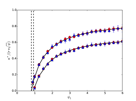
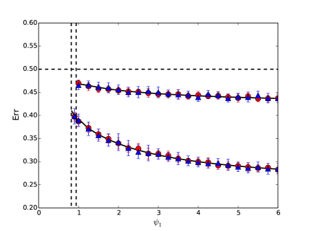
Figure 1: Random features model, with ReLU activations. Left: maximum margin. Right: test error. Labels are generated using the logistic function $f(x)=(1+e^{-\beta x})^{-1}$ with $\beta=1,4$ (bottom to top on the left and top to bottom on the right). Here $\psi_{2}=n/d=2$, and red circles, blue triangles stand for $d=400,200$ respectively. Results were averaged over $20$ samples, Dashed lines report the interpolation threshold, and continuous lines are the predicted test error, both within the Gaussian covariates model of Section 3.2.

A

Figure 2: Random features model, with ReLU activations. Recall the notation $\psi_{1}$ and $\psi_{2}$ from (3.4). Left: maximum margin. Right: test error. Labels are generated using the logistic function $f(x)=(1+e^{-\beta x})^{-1}$ with $\beta=4$. Here red circles stand for empirical values for $d=400$, and results were averaged over $20$ samples. Blue surfaces are the predicted values, both within the Gaussian covariates model of Section 3.2.

A

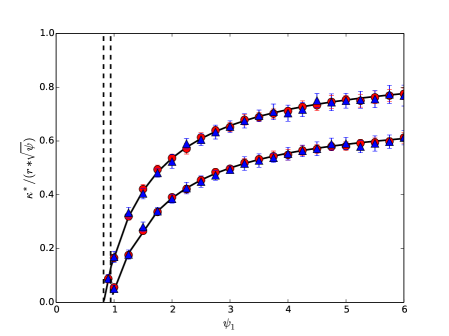
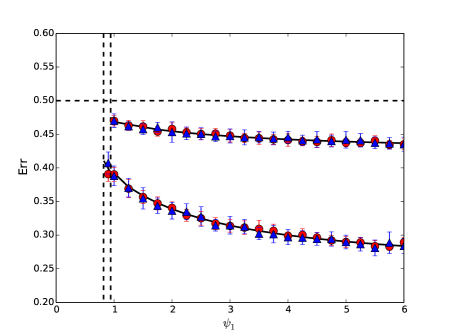
Figure 3: Random features model: same setting as in Figure 1, for a different activation function $\sigma_{1}(x)$ (see text). This activation is expected to have asymptotically the same maximum margin and test error as ReLU.

In Figures 1, 2 we report the results of numerical simulations within the random features model with ReLU activations. We compare the outcome of these simulation with the analytical predictions of Theorem 2. The agreement is excellent already at moderate values of $n,p,d$.

• Vertical lines correspond to the analytical predictions for the interpolation threshold $\psi^{*}$. For $p/n\to\psi_{1}/\psi_{2}>\psi^{*}$ the data have (With high probability) a strictly positive margin. Indeed the margin appears to vanish linearly as $p/n$ approaches $\psi^{*}$.

• The test error is monotonically decreasing with the overparametrization ratio $p/n=\psi_{1}/\psi_{2}$, and its global minimum is achieved at large overparametrization $\psi_{1}/\psi_{2}\gg 1$.

• The margin is monotonically increasing in $\psi$ for $\psi>\psi^{*}$.

At first sight, the last two observations might suggest that the decrease of test error can be explained by the increase of the margin using standard margin theory. In order to understand whether this is the case, we consider for instance [SSBD14, Theorem 26.14], which implies, with our notations,

$${\rm Err}_{n}({\boldsymbol{y}},{\boldsymbol{X}})\leq\frac{4r\sqrt{\psi}}{\kappa^{*}(\psi)}+o_{n}(1)\,,\;\;\;\;\;r^{2}:=\int x\,\mu({\rm d}x,{\rm d}w)\,.$$ (3.24)

Here $r$ is the typical radius of the feature vectors, namely the asymptotic value of $r_{n}^{2}=\mathbb{E}\|{\boldsymbol{x}}_{1}\|^{2}/p$, (in the ReLU case, $r=1/\sqrt{2}$). Even discarding the factor $4$ (which we do in Figure 6), this upper bound has the wrong qualitative dependence on $\psi$ and is never non-trivial in the present setting (never smaller than 1). As it can be seen from the plots of the margin, this upper bound is is always larger than one in this application (even neglecting the factor $4$), and therefore vacuous.

One particular prediction of our theory is that the test error and the margin should depend on the activation function only through the two coefficients $\gamma_{1}$ and $\gamma_{*}$. We check this numerically by repeating the same simulation of Figure 1, but using a different activation function. Namely, we use activation $\sigma_{2}(x)=0.5x_{+}+a_{0}x_{+}^{2}+a_{1}x_{+}(1+x_{+})^{-1}$, where we choose $a_{0}$ and $a_{1}$ as to obtain the same values of $\gamma_{1},\gamma_{*}$ as for ReLU. Figure 3 reports the outcome of numerical simulations with activation $\sigma_{2}$. As conjectured, the two sets of numerical results in Figures 1 and 3 are hardly distinguishable.

3.4 Wide network asymptotics

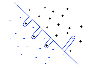
Figure 4: A cartoon of random features max margin classifiers. This is a pictorial representation of Proposition 3.2. The random features classifier (continuous line) achieves vanishing training error, but behaves as a linear classifier with a soft margin (dotted line).

Of particular interest for the random features model is the wide network asymptotics $\psi_{1}\to\infty$, at fixed $\psi_{2}$. This corresponds to a large number of neurons per dimension ($p/d$ large), while the number of samples per dimension $n/d$ stays constant. It is important to bear in mind that these limits are taken after $p,n,d\to\infty$ with $p/d=\psi_{1}$, $n/d=\psi_{2}$: hence $p/d$ should be interpreted here as large but of order one.

The next proposition characterizes this limit: its proof is deferred to Appendix J.

Proposition 3.1.

Let $\kappa^{*}(\mu_{\psi_{1}},\psi)$, ${\rm Err}^{*}(\mu_{\psi_{1}},\psi)$ be the asymptotic maximum margin and classification error of the random features model defined in Section 3.1, cf. Theorem 2. For $\psi_{2},\gamma_{1},\gamma_{*}>0$, define $T_{\infty}(\,\cdot\,;\psi_{2},\gamma_{1},\gamma_{*}):\mathbb{R}_{>0}\to\mathbb{R}$ by

$$T_{\infty}(\bar{\kappa};\psi_{2},\gamma_{1},\gamma_{*})=\min_{\begin{subarray}{c}d_{1}^{2}+d_{2}^{2}\leq 1,\\ d_{2}\geq 0\end{subarray}}\bigg{\{}F_{\bar{\kappa}}(\sqrt{\psi_{2}}\gamma_{1}d_{1},\sqrt{\psi_{2}}\gamma_{1}d_{2})-\gamma_{1}d_{2}-\gamma_{*}\sqrt{1-d_{1}^{2}-d_{2}^{2}}\bigg{\}}\,.$$ (3.25)

where $F_{\kappa}$ is defined in Eq. (5.1) below. Denote the unique minimizer of this optimization problem by $(d_{1}^{*},d_{2}^{*})=(d_{1}^{*}(\bar{\kappa}),d_{2}^{*}(\bar{\kappa}))$, and let

$$\bar{\kappa}^{*,{\mbox{\rm\tiny wide}}}(\psi_{2},\gamma_{1},\gamma_{*})\equiv\inf\big{\{}\bar{\kappa}>0:\;\;T_{\infty}(\bar{\kappa};\psi_{2},\gamma_{1},\gamma_{*})=0\big{\}}\,.$$ (3.26)

Finally define $d_{i}^{*,{\mbox{\rm\tiny wide}}}=d_{i}^{*}(\bar{\kappa}^{*,{\mbox{\rm\tiny wide}}})$ and

$${\rm Err}^{*,{\mbox{\rm\tiny wide}}}(\psi_{2},\gamma_{1},\gamma_{*})\equiv\mathbb{P}\left(\nu^{*,{\mbox{\rm\tiny wide}}}Y_{0}G+\sqrt{1-(\nu^{*,{\mbox{\rm\tiny wide}}})^{2}}Z\leq 0\right)\,,$$ (3.27)

$$\nu^{*,{\mbox{\rm\tiny wide}}}=\nu^{*,{\mbox{\rm\tiny wide}}}(\psi_{2},\gamma_{1},\gamma_{*})=\frac{d_{1}^{*,{\mbox{\rm\tiny wide}}}}{\sqrt{(d_{1}^{*,{\mbox{\rm\tiny wide}}})^{2}+(d_{2}^{*,{\mbox{\rm\tiny wide}}})^{2}}},\leavevmode\nobreak\ \leavevmode\nobreak\ \text{where}\leavevmode\nobreak\ \leavevmode\nobreak\ d_{i}^{*,{\mbox{\rm\tiny wide}}}=d_{i}^{*}(\bar{\kappa}^{*,{\mbox{\rm\tiny wide}}})\leavevmode\nobreak\ \leavevmode\nobreak\ \text{for}\leavevmode\nobreak\ \leavevmode\nobreak\ i=1,2\,,$$ (3.28)

where expectation is with respect to $Z$ independent of $(Y_{0},G)$, $\mathbb{P}(Y_{0}=+1\mid G)=h(G)$, $\mathbb{P}(Y_{0}=-1\mid G)=1-h(G)$, $Z,G\stackrel{{\scriptstyle i.i.d}}{{\sim}}\mathsf{N}(0,1)$.

Then

$$\lim_{\psi_{1}\to\infty}\frac{\kappa^{*}(\mu_{\psi_{1}},\psi))}{\sqrt{\psi}} =\bar{\kappa}^{*,{\mbox{\rm\tiny wide}}}(\psi_{2},\gamma_{1},\gamma_{*})\,,$$ (3.29)

$$\lim_{\psi_{1}\to\infty}{\rm Err}^{*}(\mu_{\psi_{1}},\psi) ={\rm Err}^{*,{\mbox{\rm\tiny wide}}}(\psi_{2},\gamma_{1},\gamma_{*})\,.$$ (3.30)

It turns out that Proposition 3.1 has a remarkably simple interpretation. In the wide, high-dimensional limit, the random features model behaves as a simple linear model in the covariates ${\boldsymbol{z}}_{i}$, whereby instead of the maximum margin classifier of Eq. (1.4), we solve the following soft margin problem

$$(\hat{\boldsymbol{\theta}}^{\mbox{\tiny\rm SM}},\hat{\boldsymbol{u}}^{\mbox{\tiny\rm SM}})\in\mathop{\rm argmax}_{{\boldsymbol{\theta}}\in\mathbb{R}^{d},\,{\boldsymbol{u}}\in\mathbb{R}^{n}}\left\{\min_{i\leq n}\big{[}\gamma_{1}y_{i}\langle{\boldsymbol{\theta}},{\boldsymbol{z}}_{i}\rangle+\gamma_{*}u_{i}\big{]}\;:\;\;\;\|{\boldsymbol{\theta}}\|_{2}^{2}+\frac{\|{\boldsymbol{u}}\|_{2}^{2}}{d}=1\right\}\,.$$ (3.31)

We denote by $\kappa_{n}^{\mbox{\tiny\rm SM}}({\boldsymbol{y}},{\boldsymbol{Z}})$ the corresponding soft margin, namely the value of this optimization problem. (Here ${\boldsymbol{Z}}\in\mathbb{R}^{n\times d}$ is the matrix whose $i$-th row is ${\boldsymbol{z}}_{i}$.)

Proposition 3.2.

Let $\bar{\kappa}^{*,{\mbox{\rm\tiny wide}}}(\psi_{2},\gamma_{1},\gamma_{*})$, ${\rm Err}^{*,{\mbox{\rm\tiny wide}}}(\psi_{2},\gamma_{1},\gamma_{*})$ be the asymptotic margin and classification error of the noisy linear features model, as defined in Proposition 3.1, Eqs. (3.26), (3.27). Further, denote by $\kappa_{n}^{\mbox{\tiny\rm SM}}({\boldsymbol{y}},{\boldsymbol{Z}})$ the soft-margin, that is the optimum value of problem (3.31), and ${\rm Err}_{n}^{\mbox{\tiny\rm SM}}({\boldsymbol{y}},{\boldsymbol{Z}})$ the corresponding classification error. Consider the proportional asymptotics $n,d\to\infty$ with $n/d\to\psi_{2}\in(0,\infty)$. Then

$$\lim_{n\to\infty}\kappa_{n}^{\mbox{\tiny\rm SM}}({\boldsymbol{y}},{\boldsymbol{Z}})=\frac{\bar{\kappa}^{*,{\mbox{\rm\tiny wide}}}(\psi_{2},\gamma_{1},\gamma_{*})}{\sqrt{\psi_{2}}}\,,\;\;\;\;\;\;\;\;\;\lim_{n\to\infty}{\rm Err}_{n}^{\mbox{\tiny\rm SM}}({\boldsymbol{y}},{\boldsymbol{Z}})={\rm Err}^{*,{\mbox{\rm\tiny wide}}}(\psi_{2},\gamma_{1},\gamma_{*})\,.$$ (3.32)

The proof of Proposition 3.2 is deferred to Appendix K.

Remark 3.2.

It is worth emphasizing that Proposition 3.2 establishes the equivalence of two classifiers that —at first sight— are very different. The first one is the original random features max-margin classifier which is linear in the $p$-dimensional lifted space, but non-linear in the underlying $d$-dimensional space, and has vanishing training error. The second one is the soft-margin classifier of Eq. (3.31). This is a linear classifier in $d$ dimensions. A pictorial representation of this result is given in Figure 4.

4 Further related work

‘Noisy’ high-dimensional statistics.

Classical high-dimensional statistics [BVDG11] studies the regime $n\lesssim p$ but under the assumption that the parameters’ vector is highly structured. For instance, the sparsity $s_{0}$ is assumed satisfy $s_{0}\ll n/\log p$. Concentration of measure is sufficient to prove consistency in such highly structured problems.

The present work contributes to a growing body of work focuses on a different ‘noisy high-dimensional regime’ In this setting, the sample size is proportional to the number of parameters, and the estimation error (suitably rescaled) converges to a non-trivial limit [Mon18]. Asymptotically exact results have been obtained in a large array of problems including sparse regression using $\ell_{1}$ penalization (Lasso) [BM12, MM18], general regularized linear regression [DJM13, ALMT14, TOH15], robust regression [EKBB⁺13, DM16, EK18, TAH18], Bayesian estimation within generalized linear models [BKM⁺19], logistic regression [CS18, SC19], low rank matrix estimation [DAM16, LM19, BDM⁺18], and so on. Several new mathematical techniques have been developed to address this regime: constructive methods based on message passing algorithms [BM11, BLM15]; Gaussian comparison methods based on Gordon’s inequality [Gor88, TOH15]; interpolation techniques motivated from statistical physics [BM19].

The study of this ‘noisy high-dimensional’ regime has a long history in statistical physics. Non-rigorous methods from spin glass theory have been successfully used since the eighties in this context. We refer to [EVdB01] for an overview of this early work, and to [MPV87, MM09] for general introductions. An early breakthrough in this line of work was the result by Elizabeth Gardner [Gar88], who computed the maximum margin $\kappa^{*}(\psi)$ for the special case of isotropic features and purely random labels (i.e. ${\boldsymbol{\Sigma}}_{n}={\boldsymbol{I}}_{p}$ and $f(x)=1/2$).

Here we follow the approach based on Gordon’s inequality [Gor88], as formalized by Thrampoulidis, Oymak, Hassibi [TOH15]. Gordon’s inequality was previously used to study various statistical learning problems such as compressed sensing [Sto10, CRPW12] and Lasso [Sto13, OTH13]. The closest results to ours in the earlier literature are the analysis of logistic regression by Sur and Candés [CS18, SC19], and the recent paper on regularized logistic regression by Salehi, Abbasi and Hassibi [SAH19]. Both of these analyses focus on the underparametrized regime, in which the maximum likelihood estimator is well defined and (with high probability) unique. By contrast, we focus on the overparametrized regime here. Further, while earlier work assumes isotropic covariates ${\boldsymbol{x}}_{i}\sim\mathsf{N}(0,{\boldsymbol{I}}_{p})$, we consider a general covariance structure, under Assumptions 1 and 2. This is crucial in order to be able to capture the behavior of overparametrized random features models. From a technical point of view, our approach is related to the one of [SAH19]. Notice however that [SAH19] does not prove uniqueness of the minimizer of Gordon’s optimization problem, while this is the main technical challenge that we address in our proof (in a more complicated setting, due to the general covariance).

Overparametrization and overfitting.

As discussed in the introduction, our work is connected to a substantial line of research that investigates the behavior of generalization error in overparametrized model that interpolate the data. This work was largely motivated by the empirical observation that deep neural networks fit perfectly the data and yet generalize well [ZBH⁺16, NBMS17]. It was noticed in [BMM18] that this behavior is significantly more general than neural networks, while [BHMM19] pointed out that the classical U-shaped curve describing the behavior of generalization error as a function of number of parameters does not hold in general. Independently, [GJS⁺19] observed the same phenomenon in the context of multilayer networks, and connected it to phase transitions in physics.

Mathematical results about generalization behavior in the overparametrized regime have been obtained in several recent papers [BHM18, BHX19, LR20, RZ18, MVS19, HMRT22, BLLT20, MM19]. However, all of earlier work has focused on least squares (or ridge) regression with square loss. (Certain nearest-neighbor-like methods are also considered in [BHM18].) The closest earlier results in this literature are [HMRT22, MM19] which use random matrix theory to characterize ridge regression in the proportional asymptotics $p,n\to\infty$ with $p/n=\psi$. Moving beyond ridge regression requires abandoning the powerful tools of random matrix theory and developing new mathematical tools.

Threshold for linear separability.

As a corollary of our theory, we characterize a the threshold for linear separability $\psi^{*}=\psi^{*}(f)$. For $p/n\to\psi>\psi^{*}$ data are with high probability separable (with a margin bounded away from $0$), while for $p/n\to\psi<\psi^{*}$ they are not. A classical result of Cover [Cov65] yields $\psi^{*}=1/2$ for the special case in which $y_{i}\sim{\sf Unif}(\{+1,-1\})$ independently of ${\boldsymbol{x}}_{i}$, provided the $({\boldsymbol{x}}_{i})_{i\leq n}$ are in generic positions. This result was recently generalized by Candés and Sur [CS18] for the more challenging setting in which $\mathbb{P}(y_{i}=+1|{\boldsymbol{x}}_{i})=(1+e^{-\langle{\boldsymbol{\theta}}_{*},{\boldsymbol{x}}_{i}\rangle})^{-1}$ and ${\boldsymbol{x}}_{i}$ is Gaussian. Our results yield a generalization of the threshold obtained in [CS18], but also characterize the margin in the overparametrized regime $\psi>\psi^{*}$. (The latter is significantly more challenging because the margin depends on all the entries of $({\boldsymbol{\Sigma}},{\boldsymbol{\theta}}_{*})$ while the separability does not.)

Independent and follow-up work.

The special case of isotropic covariates ${\boldsymbol{\Sigma}}={\boldsymbol{I}}_{p}$ was treated independently from our work in [DKT22].

After the first version of this paper was posted online, our results were generalized in a number of significant ways by several authors. A few pointers to this literature are [GMKZ20, KT20, TPT20, GLK⁺20, KPOT21, LS22, JS22] (we limit ourselves to papers that derive sharp asymptotics in the proportional regime). The most closely related work is [LS22] that adapts the techniques of the present paper to analyze max $\ell_{1}$-margin (rather than max $\ell_{2}$ as we do here).

Non-asymptotic bounds on max-margin classification were proven in [CL21], implying benign overfitting in certain settings in certain settings. Namely, the data distribution is a mixture $(\mathbb{P}_{+}+\mathbb{P}_{-})/2$ where $\mathbb{P}_{+}({\boldsymbol{x}}_{i}\in\,\cdot\,)$ and $\mathbb{P}_{-}({\boldsymbol{x}}_{i}\in\,\cdot\,)$ are assumed to be well separated, and labels noise is independent of the features: $\mathbb{P}_{+}(y_{i}=-1|{\boldsymbol{x}}_{i})=\mathbb{P}_{-}(y_{i}=+1|{\boldsymbol{x}}_{i})=\eta$ independent of ${\boldsymbol{x}}_{i}$. This analysis was generalized to two-layer ReLU networks in [FCB22, FVBS23].

Finally, the recent paper [ZKS⁺22] (building on the earlier work [KZSS21]) obtains non-asymptotic bound on population loss in generalized linear models. Their approach also uses Gaussian comparison inequalities as ours and imply certain benign overfitting guarantees.

While limited to proportional asymptotics, our work is the first one characterizing covariances and parameters’ sequences $({\boldsymbol{\Sigma}},{\boldsymbol{\theta}}_{*})$ under which max-margin classification displays benign overfitting in classification accuracy.

5 Main results

Our main technical theorem characterizes the asymptotic value of the maximum margin $\kappa^{*}(\mu,\psi)$ and the asymptotic generalization error of the max-margin classifier, to be denoted by ${\rm Err}^{*}(\mu,\psi)$.

5.1 Introducing the asymptotic predictions

We start by defining our general analytical predictions $\kappa^{*}(\mu,\psi)$ and ${\rm Err}^{*}(\mu,\psi)$. Recall that $\rho\in\mathbb{R}_{>0}$ and the probability measure $\mu$ on $\mathbb{R}_{>0}\times\mathbb{R}$ are defined by Assumption 2. For any $\kappa\geq 0$, define $F_{\kappa}:\mathbb{R}\times\mathbb{R}_{\geq 0}\to\mathbb{R}_{\geq 0}$ by

$$F_{\kappa}(c_{1},c_{2})=\left(\mathbb{E}\left[(\kappa-c_{1}YG-c_{2}Z)_{+}^{2}\right]\right)^{1/2}\leavevmode\nobreak\ \leavevmode\nobreak\ \text{where}\leavevmode\nobreak\ \begin{cases}Z\perp(Y,G)\\ Z\sim\mathsf{N}(0,1),G\sim\mathsf{N}(0,1)\\ \mathbb{P}(Y=+1\mid G)=f(\rho\cdot G)\\ \mathbb{P}(Y=-1\mid G)=1-f(\rho\cdot G)\end{cases}$$ (5.1)

Let the random variables $X,W$ be such that $(X,W)\sim\mu$. Introduce the constants

$$\zeta=\left(\mathbb{E}_{\mu}[X^{-1}W^{2}]\right)^{-1/2}\leavevmode\nobreak\ \text{and}\leavevmode\nobreak\ \omega=\left(\mathbb{E}_{\mu}[(1-\zeta^{2}X^{-1})^{2}W^{2}]\right)^{1/2}.$$ (5.2)

Define the functions $\psi_{+}:\mathbb{R}_{>0}\to\mathbb{R}$  and $\psi_{-}:\mathbb{R}_{>0}\to\mathbb{R}$ by

$$\begin{split}\psi_{+}(\kappa)&=\begin{cases}0\leavevmode\nobreak\ \leavevmode\nobreak\ &\text{if $\partial_{1}F_{\kappa}(\zeta,0)>0$,}\\ \partial_{2}^{2}F_{\kappa}(\zeta,0)-\omega^{2}\partial_{1}^{2}F_{\kappa}(\zeta,0)\leavevmode\nobreak\ \leavevmode\nobreak\ \leavevmode\nobreak\ \leavevmode\nobreak\ \leavevmode\nobreak\ \leavevmode\nobreak\ \leavevmode\nobreak\ &\text{if otherwise,}\end{cases}\\ \psi_{-}(\kappa)&=\begin{cases}0\leavevmode\nobreak\ \leavevmode\nobreak\ &\text{if $\partial_{1}F_{\kappa}(-\zeta,0)>0$,}\\ \partial_{2}^{2}F_{\kappa}(-\zeta,0)-\omega^{2}\partial_{1}^{2}F_{\kappa}(-\zeta,0)\leavevmode\nobreak\ \leavevmode\nobreak\ &\text{if otherwise.}\end{cases}\end{split}$$ (5.3)

Finally, we define $\psi^{*}(0)$ and $\psi^{\downarrow}:\mathbb{R}_{>0}\to\mathbb{R}_{\geq 0}$ by

$$\psi^{*}(0) =\min_{c\in\mathbb{R}}F_{0}^{2}(c,1)\,,$$ (5.4)

$$\psi^{\downarrow}(\kappa) =\max\{\psi^{*}(0),\psi_{+}(\kappa),\psi_{-}(\kappa)\}.$$ (5.5)

The next proposition guarantees that the definition of $\kappa^{*}(\mu,\psi)$, and ${\rm Err}^{*}(\mu,\psi)$ given below are meaningful. Its proof is deferred to Appendix B. In the following, we will often omit the argument $\mu$ from $\kappa^{*}$, ${\rm Err}^{*}$, $\mathcal{L}^{*}$.

Proposition 5.1.

1. For any $\psi>\psi^{\downarrow}(\kappa)$, the following system of equations has unique solution $(c_{1},c_{2},s)\in\mathbb{R}\times\mathbb{R}_{>0}\times\mathbb{R}_{>0}$ (here expectation is taken with respect to $(X,W)\sim\mu$):

   $$\begin{split}-c_{1}&=\mathbb{E}_{\mu}\left[\frac{\left(\partial_{1}F_{\kappa}(c_{1},c_{2})-c_{1}c_{2}^{-1}\partial_{2}F_{\kappa}(c_{1},c_{2})\right)W^{2}X^{1/2}}{c_{2}^{-1}\partial_{2}F_{\kappa}(c_{1},c_{2})X^{1/2}+\psi^{1/2}sX^{-1/2}}\right]\,,\\ c_{1}^{2}+c_{2}^{2}&=\mathbb{E}_{\mu}\left[\frac{\psi X+\left(\partial_{1}F_{\kappa}(c_{1},c_{2})-c_{1}c_{2}^{-1}\partial_{2}F_{\kappa}(c_{1},c_{2})\right)^{2}W^{2}X}{(c_{2}^{-1}\partial_{2}F_{\kappa}(c_{1},c_{2})X^{1/2}+\psi^{1/2}sX^{-1/2})^{2}}\right]\,,\\ 1&=\mathbb{E}_{\mu}\left[\frac{\psi+\left(\partial_{1}F_{\kappa}(c_{1},c_{2})-c_{1}c_{2}^{-1}\partial_{2}F_{\kappa}(c_{1},c_{2})\right)^{2}W^{2}}{(c_{2}^{-1}\partial_{2}F_{\kappa}(c_{1},c_{2})X^{1/2}+\psi^{1/2}sX^{-1/2})^{2}}\right]\,.\end{split}$$ (5.6)

2. Define the function $T:(\psi,\kappa)\to\mathbb{R}$ (for any $\psi>\psi^{\downarrow}(\kappa)$) by

   $$T(\psi,\kappa)=\psi^{-1/2}\left(F_{\kappa}(c_{1},c_{2})-c_{1}\partial_{1}F_{\kappa}(c_{1},c_{2})-c_{2}\partial_{2}F_{\kappa}(c_{1},c_{2})\right)-s\,,$$ (5.7)

   where $(c_{1}(\psi,\kappa),c_{2}(\psi,\kappa),s(\psi,\kappa))$ is the unique solution of Eq (5.6) in $\mathbb{R}\times\mathbb{R}_{>0}\times\mathbb{R}_{>0}$. Then we have

   1. $T(\cdot,\cdot),c_{1}(\cdot,\cdot),c_{2}(\cdot,\cdot),s(\cdot,\cdot)$ are continuous functions in the domain $\left\{(\psi,\kappa):\psi>\psi^{\downarrow}(\kappa)\right\}$.

   2. For any $\kappa>0$, the mapping $T(\,\cdot\,,\kappa)$ is strictly monotonically decreasing, and satisfies

      $$\lim_{\psi\nearrow+\infty}T(\psi,\kappa)<0<\lim_{\psi\searrow\psi^{\downarrow}(\kappa)}T(\psi,\kappa).$$ (5.8)

   3. For any $\psi>0$, the mapping $T(\psi,\cdot)$ is strictly monotonically increasing, and satisfies

      $$\lim_{\kappa\nearrow+\infty}T(\psi,\kappa)=\infty.$$ (5.9)

We are now in position to define $\kappa^{*}(\mu,\psi)$, ${\rm Err}^{*}(\mu,\psi)$ and $\mathcal{L}^{*}(\mu,\psi)$.

Definition 5.1.

Recall the function $T$ defined at Eq. (5.7). For any $\psi\geq\psi^{*}(0)$, we define the asymptotic max-margin as

$$\kappa^{*}(\mu,\psi)=\inf\left\{\kappa\geq 0:T(\psi,\kappa)=0\right\}.$$

We further define the asymptotic generalization error ${\rm Err}^{*}:(0,\infty)\to[0,1]$ by

$${\rm Err}^{*}(\mu,\psi) =\mathbb{P}\left(\nu^{*}(\psi)YG+\sqrt{1-\nu^{*}(\psi)^{2}}Z\leq 0\right)\,,$$ (5.10)

$$\nu^{*}(\psi) \equiv\frac{c_{1}^{*}(\psi)}{\sqrt{(c_{1}^{*}(\psi))^{2}+(c_{2}^{*}(\psi))^{2}}}\,,$$ (5.11)

where probability is over $Z\perp(Y,G)$, with $G,Z\sim\mathsf{N}(0,1)$ and $\mathbb{P}(Y=+1\mid G)=f(\rho\cdot G)=1-\mathbb{P}(Y=-1\mid G)$. Further $c_{i}^{*}(\psi)=c_{i}(\psi,\kappa^{*}(\psi))$, $i\in\{1,2\}$. Lastly, for each $\psi>\psi^{\downarrow}(\kappa)$, we introduce the random variable

$$H_{\psi,\kappa}(G,X,W)=-\frac{\psi^{1/2}G+\left(\partial_{1}F_{\kappa}(c_{1},c_{2})-c_{1}c_{2}^{-1}\partial_{2}F_{\kappa}(c_{1},c_{2})\right)W}{c_{2}^{-1}\partial_{2}F_{\kappa}(c_{1},c_{2})X^{1/2}+\psi^{1/2}sX^{-1/2}}.$$ (5.12)

where $(c_{1},c_{2},s)$ is defined as in Proposition 5.1. We use $\mathcal{L}_{\psi,\kappa}$ to denote the distribution of the random variable $(X,W,H_{\psi,\kappa}(G,X,W))$ when $(G,X,W)\sim\mathsf{N}(0,1)\otimes\mu$. Define

$$\mathcal{L}^{*}(\mu,\psi)=\mathcal{L}_{\psi,\kappa^{*}(\psi)}.$$

Proposition 5.1 shows that the mapping $\psi\to\kappa^{*}(\mu,\psi)$ is well-defined, strictly monotonically increasing, and satisfies $\lim_{\psi\to\infty}\kappa^{*}(\mu,\psi)=\infty$.

5.2 Main statement

Below we present the main mathematical result of this paper. Section 6 presents the proof of this theorem, with most technical legwork deferred to the appendices.

Theorem 3.

Consider i.i.d. data $({\boldsymbol{y}},{\boldsymbol{X}})=\{(y_{i},{\boldsymbol{x}}_{i})\}_{i\leq n}$ where ${\boldsymbol{x}}_{i}\sim\mathsf{N}({\boldsymbol{0}},{\boldsymbol{\Sigma}}_{n})$ and $\mathbb{P}\big{(}y_{i}=+1\big{|}{\boldsymbol{x}}_{i}\big{)}=f(\langle{\boldsymbol{\theta}}_{*,n},{\boldsymbol{x}}_{i}\rangle)$. Assume $n,p\to\infty$ with $p/n\to\psi\in(0,\infty)$, and ${\boldsymbol{\theta}}_{*,n},{\boldsymbol{\Sigma}}_{n},f$ satisfying Assumptions 1, 2, 3. (In particular, $\rho,\mu$ are defined by Assumption 2.)

Let $\psi^{*}(0)$ be defined as per Eq. (5.4), and $\kappa^{*}(\mu,\psi)$, ${\rm Err}^{*}(\mu,\psi)$ be determined as per Definition 5.1. Then the following hold:

1. With probability tending to one, the data are linearly separable if $\psi>\psi^{*}(0)$ and are not linearly separable if $\psi<\psi^{*}(0)$.

2. Let $\kappa_{n}({\boldsymbol{y}},{\boldsymbol{X}})\equiv\max_{\|{\boldsymbol{\theta}}\|_{2}=1}\min_{i\leq n}y_{i}\langle{\boldsymbol{\theta}},{\boldsymbol{x}}_{i}\rangle$ be the maximum margin for data $({\boldsymbol{y}},{\boldsymbol{X}})$. In the overparametrized regime $\psi>\psi^{*}(0)$ we have, as $n\to\infty$,

   $$\kappa_{n}({\boldsymbol{y}},{\boldsymbol{X}})\stackrel{{\scriptstyle p}}{{\to}}\kappa^{*}(\mu,\psi)\,.$$ (5.13)

3. Let ${\rm Err}_{n}({\boldsymbol{y}},{\boldsymbol{X}})\equiv\mathbb{P}\big{(}y^{\mbox{\tiny\rm new}}\langle\hat{\boldsymbol{\theta}}^{\mbox{\tiny\rm MM}}({\boldsymbol{y}},{\boldsymbol{X}}),{\boldsymbol{x}}^{\mbox{\tiny\rm new}}\rangle\leq 0\big{)}$ be the prediction error of the maximum margin classifier. In the overparametrized regime $\psi>\psi^{*}(0)$ we have, as $n\to\infty$,

   $${\rm Err}_{n}({\boldsymbol{y}},{\boldsymbol{X}})\stackrel{{\scriptstyle p}}{{\to}}{\rm Err}^{*}(\mu,\psi)\,.$$ (5.14)

4. Recall that $\{\lambda_{i}\}_{i\in[p]}$, $\{{\boldsymbol{v}}_{i}\}_{i\in[p]}$ are the eigenvalues and eigenvectors of ${\boldsymbol{\Sigma}}_{n}$ and $\bar{w}_{i}=\sqrt{p\lambda_{i}}\langle{\boldsymbol{v}}_{i},{\boldsymbol{\theta}}_{*,n}\rangle/\rho_{n}$ for $\rho_{n}=\langle{\boldsymbol{\theta}}_{*,n},{\boldsymbol{\Sigma}}_{n}{\boldsymbol{\theta}}_{*,n}\rangle^{1/2}$ (see Section 1.2). Let $\hat{\mathcal{L}}_{n}({\boldsymbol{y}},{\boldsymbol{X}})$ denote the empirical distribution induced by $\{(\lambda_{i},\bar{w}_{i},\sqrt{p}\langle\hat{{\boldsymbol{\theta}}}_{n}^{{\mbox{\tiny\rm MM}}},{\boldsymbol{v}}_{i}\rangle)\}_{i\in[p]}$, i.e., $\hat{\mathcal{L}}_{n}({\boldsymbol{y}},{\boldsymbol{X}})=\frac{1}{p}\sum_{i=1}^{p}\delta_{(\lambda_{i},\bar{w}_{i},\sqrt{p}\langle\hat{{\boldsymbol{\theta}}}_{n}^{{\mbox{\tiny\rm MM}}},{\boldsymbol{v}}_{i}\rangle)}.$ In the overparametrized regime $\psi>\psi^{*}(0)$ we have, as $n\to\infty$,

   $$W_{2}\left(\hat{\mathcal{L}}_{n}({\boldsymbol{y}},{\boldsymbol{X}}),\mathcal{L}^{*}(\mu,\psi)\right)\stackrel{{\scriptstyle p}}{{\to}}0.$$ (5.15)

Remark 5.1.

Point $(a)$ in Theorem 3 is a generalization of the recent result of [CS18], which concerns the case in which $f(x)$ is a logistic function.

The main content of Theorem 3 is in parts $(b)$, $(c)$ and $(d)$. To the best of our knowledge, the only case that had been characterized before is the one of isotropic covariates and purely random labels (i.e. ${\boldsymbol{\Sigma}}_{n}={\boldsymbol{I}}_{p(n)}$ and $f(x)=1/2$). In this case the asymptotic value of the maximum margin was first determined rigorously by Shcherbina and Tirozzi [ST03], confirming the non-rigorous result by Gardner [Gar88].

5.3 Proof technique

Parts $(a)$, $(b)$. Consider first the problem of determining the asymptotics of the maximum margin. Recall that ${\boldsymbol{X}}\in\mathbb{R}^{n\times p}$ denotes the matrix with rows ${\boldsymbol{x}}_{1},\dots,{\boldsymbol{x}}_{n}$ and, for any $\kappa>0$, define the event

$$\mathcal{E}_{n,\psi,\kappa}=\left\{\exists{\boldsymbol{\theta}}\in\mathbb{R}^{p},\leavevmode\nobreak\ \left\|{{\boldsymbol{\theta}}}\right\|_{2}\leq 1,\text{such that}\leavevmode\nobreak\ y_{i}\langle{\boldsymbol{x}}_{i},{\boldsymbol{\theta}}\rangle\geq\kappa\leavevmode\nobreak\ \text{for $i\in[n]$}\right\}.$$

In order to prove Theorem 3.$(b)$, we would like to determine for which pairs $(\psi,\kappa)$ we have $\mathbb{P}(\mathcal{E}_{n,\psi,\kappa})\to 1$ and for which pairs instead $\mathbb{P}(\mathcal{E}_{n,\psi,\kappa})\to 0$.

To this end, we define $\xi_{n,\psi,\kappa}$ by

$$\xi_{n,\psi,\kappa}=\min_{\left\|{{\boldsymbol{\theta}}}\right\|_{2}\leq 1}\leavevmode\nobreak\ \max_{\left\|{{\boldsymbol{\lambda}}}\right\|_{2}\leq 1,{\boldsymbol{y}}\odot{\boldsymbol{\lambda}}\geq 0}\frac{1}{\sqrt{p}}{\boldsymbol{\lambda}}^{{\sf T}}(\kappa{\boldsymbol{y}}-{\boldsymbol{X}}{\boldsymbol{\theta}})\,.$$ (5.16)

We then have:

$$\left\{\xi_{n,\psi,\kappa}>0\right\}\Leftrightarrow\mathcal{E}^{c}_{n,\psi,\kappa}\leavevmode\nobreak\ \leavevmode\nobreak\ \text{and}\leavevmode\nobreak\ \leavevmode\nobreak\ \left\{\xi_{n,\psi,\kappa}=0\right\}\Leftrightarrow\mathcal{E}_{n,\psi,\kappa}\,.$$ (5.17)

This equivalence follows immediately from the following identities

$$\mathcal{E}_{n,\psi,\kappa} =\left\{\exists{\boldsymbol{\theta}}\in\mathbb{R}^{p},\left\|{{\boldsymbol{\theta}}}\right\|_{2}\leq 1\leavevmode\nobreak\ \text{such that }\left\|{(\kappa\textbf{1}-({\boldsymbol{y}}\odot{\boldsymbol{X}}{\boldsymbol{\theta}}))_{+}}\right\|_{2}=0\right\}\,,$$

$$\xi_{n,\psi,\kappa} =\min_{\left\|{{\boldsymbol{\theta}}}\right\|_{2}\leq 1}\leavevmode\nobreak\ \frac{1}{\sqrt{p}}\left\|{(\kappa\textbf{1}-({\boldsymbol{y}}\odot{\boldsymbol{X}}{\boldsymbol{\theta}}))_{+}}\right\|_{2}\,.$$

We are then reduced to study the typical value of the minimax problem (5.16). Notice that this problem is convex in ${\boldsymbol{\theta}}$, concave in ${\boldsymbol{\lambda}}$, and linear in the Gaussian random matrix ${\boldsymbol{X}}$. We use Gordon’s Gaussian comparison inequality [Gor88] (and in particular a refinement due to Thrampoulidis, Oymak, Hassibi [TOH15]) to study the asymptotics of $\xi_{n,\psi,\kappa}$.

The result on data separability (Theorem 3.$(a)$) essentially follows from the analysis of the maximum margin. First, a direct implication of Theorem 3.$(b)$ is the separability of data (with high probability) if $\psi>\psi^{*}(0)$. To show the other way around, we consider instead $\Xi_{n,\psi}$, whose definition replaces the constraint $\left\|{{\boldsymbol{\theta}}}\right\|_{2}\leq 1$ in equation (5.16) by $\left\|{{\boldsymbol{\theta}}}\right\|_{{\boldsymbol{\Sigma}}_{n}}:=\langle{\boldsymbol{\theta}},{\boldsymbol{\Sigma}}_{n}{\boldsymbol{\theta}}\rangle^{1/2}=1$ and substitutes $\kappa$ by $0$:

$$\Xi_{n,\psi}=\min_{\left\|{{\boldsymbol{\theta}}}\right\|_{{\boldsymbol{\Sigma}}_{n}}=1}\leavevmode\nobreak\ \max_{\left\|{{\boldsymbol{\lambda}}}\right\|_{2}\leq 1,{\boldsymbol{y}}\odot{\boldsymbol{\lambda}}\geq 0}-\frac{1}{\sqrt{p}}{\boldsymbol{\lambda}}^{{\sf T}}{\boldsymbol{X}}{\boldsymbol{\theta}}\,=\min_{\left\|{{\boldsymbol{\theta}}}\right\|_{{\boldsymbol{\Sigma}}_{n}}=1}\frac{1}{\sqrt{p}}\left\|{(-{\boldsymbol{y}}\odot{\boldsymbol{X}}{\boldsymbol{\theta}})_{+}}\right\|_{2}.$$ (5.18)

We can then apply the same technique as before to show the typical value of $\Xi_{n,\psi}$ is strictly positive, indicating non-separability of the data, under the situation when $\psi<\psi^{*}(0)$.

Part $(c)$. Let $G,Z$ be independent $\mathsf{N}(0,1)$. Define for $r\in\mathbb{R}_{\geq 0}$ and $\nu\in[-1,1]$ the error function:

$$Q(r,\nu)=\mathbb{P}\left(\nu YG+\sqrt{1-\nu^{2}}Z\leq 0\right)\leavevmode\nobreak\ \leavevmode\nobreak\ \text{where}\leavevmode\nobreak\ \leavevmode\nobreak\ \begin{cases}\mathbb{P}(Y=+1\mid G)=f(r\cdot G)\\ \mathbb{P}(Y=-1\mid G)=1-f(r\cdot G)\end{cases}$$ (5.19)

Note that in the expression (1.14), $y^{\mbox{\tiny\rm new}}$ depends on $\langle{\boldsymbol{\theta}}_{*,n},{\boldsymbol{x}}^{\mbox{\tiny\rm new}}\rangle$. Conditional on $({\boldsymbol{y}},{\boldsymbol{X}})$, $\langle{\boldsymbol{\theta}}_{*,n},{\boldsymbol{x}}^{\mbox{\tiny\rm new}}\rangle$ and $\langle\hat{\boldsymbol{\theta}}^{\mbox{\tiny\rm MM}}({\boldsymbol{y}},{\boldsymbol{X}}),{\boldsymbol{x}}^{\mbox{\tiny\rm new}}\rangle$ are jointly Gaussian with covariance $\langle\hat{\boldsymbol{\theta}}^{\mbox{\tiny\rm MM}},{\boldsymbol{\theta}}_{*,n}\rangle_{{\boldsymbol{\Sigma}}_{n}}:=\langle\hat{\boldsymbol{\theta}}^{\mbox{\tiny\rm MM}},{\boldsymbol{\Sigma}}_{n}{\boldsymbol{\theta}}_{*,n}\rangle$. Thus, it is straightforward to see that the generalization error of the max-margin classifier is given by

$${\rm Err}_{n}({\boldsymbol{y}},{\boldsymbol{X}})=Q\left(\left\|{{\boldsymbol{\theta}}_{*,n}}\right\|_{{\boldsymbol{\Sigma}}_{n}},\langle\hat{\boldsymbol{\theta}}^{\mbox{\tiny\rm MM}},{\boldsymbol{\theta}}_{*,n}\rangle_{{\boldsymbol{\Sigma}}_{n}}/(\left\|{{\boldsymbol{\theta}}_{*,n}}\right\|_{{\boldsymbol{\Sigma}}_{n}}\|{\hat{{\boldsymbol{\theta}}}^{\mbox{\tiny\rm MM}}}\|_{{\boldsymbol{\Sigma}}_{n}})\right)\,.$$ (5.20)

Comparing this expression to Theorem 3.$(c)$, and recalling that $\left\|{{\boldsymbol{\theta}}_{*,n}}\right\|_{{\boldsymbol{\Sigma}}_{n}}:=\langle{\boldsymbol{\theta}}_{*,n},{\boldsymbol{\Sigma}}_{n}{\boldsymbol{\theta}}_{*,n}\rangle^{1/2}\to\rho$ by Assumption 2, we see that it is sufficient to prove that for each $\psi>\psi^{*}(0)$,

$$\lim_{n\to\infty}\frac{\langle\hat{\boldsymbol{\theta}}^{\mbox{\tiny\rm MM}},{\boldsymbol{\theta}}_{*,n}\rangle_{{\boldsymbol{\Sigma}}_{n}}}{\left\|{{\boldsymbol{\theta}}_{*,n}}\right\|_{{\boldsymbol{\Sigma}}_{n}}\|{\hat{{\boldsymbol{\theta}}}^{\mbox{\tiny\rm MM}}}\|_{{\boldsymbol{\Sigma}}_{n}}}=\nu^{*}(\psi)\,,$$ (5.21)

where $\nu^{\star}(\psi)$ is defined in (5.10). To this end, we generalize the definition of $\xi_{n,\psi,\kappa}$ as follows. For any compact set ${\boldsymbol{\Theta}}_{p}\subseteq\mathbb{R}^{p}$, we define the quantity $\xi_{n,\psi,\kappa}({\boldsymbol{\Theta}}_{p})$ by

$$\xi_{n,\psi,\kappa}({\boldsymbol{\Theta}}_{p})=\min_{{\boldsymbol{\theta}}\in{\boldsymbol{\Theta}}_{p}}\leavevmode\nobreak\ \max_{\left\|{{\boldsymbol{\lambda}}}\right\|_{2}\leq 1,{\boldsymbol{y}}\odot{\boldsymbol{\lambda}}\geq 0}\frac{1}{\sqrt{p}}{\boldsymbol{\lambda}}^{{\sf T}}(\kappa{\boldsymbol{y}}-{\boldsymbol{X}}{\boldsymbol{\theta}})\,.$$ (5.22)

Notice that if $\xi_{n,\psi,\kappa}({\boldsymbol{\Theta}}_{p})>\xi_{n,\psi,\kappa}$ with high probability, then $\mathbb{P}(\hat{\boldsymbol{\theta}}^{\mbox{\tiny\rm MM}}_{n}\in{\boldsymbol{\Theta}}_{p})\to 0$ as $n\to\infty$. In order to control the left hand side of Eq. (5.21), we consider sets of the form

$${\boldsymbol{\Theta}}_{p}=\left\{{\boldsymbol{\theta}}\in\mathbb{R}^{p}:\;\|{\boldsymbol{\theta}}\|_{2}\leq 1\,,\;\;\;\frac{\langle\hat{\boldsymbol{\theta}}^{\mbox{\tiny\rm MM}},{\boldsymbol{\theta}}_{*,n}\rangle_{{\boldsymbol{\Sigma}}_{n}}}{\left\|{{\boldsymbol{\theta}}_{*,n}}\right\|_{{\boldsymbol{\Sigma}}_{n}}\|{\hat{{\boldsymbol{\theta}}}^{\mbox{\tiny\rm MM}}}\|_{{\boldsymbol{\Sigma}}_{n}}}\in J_{n}\right\}\,,$$ (5.23)

for suitable sequences of compact sets $J_{n}\subseteq\mathbb{R}$. Using Gordon’s inequality to lower bound $\xi_{n,\psi,\kappa}({\boldsymbol{\Theta}}_{p})$, we can guarantee that Eq. (5.21) holds.

6 Proofs

This section provides a complete outline of the proof of Theorem 3, deferring most technical steps to the appendices.

Notice that the definition of the joint distribution of $(y,{\boldsymbol{x}})$ and the statements in Theorem 3 are independent of the choice of a basis on $\mathbb{R}^{p}$. We can therefore work in the basis in which ${\boldsymbol{\Sigma}}$ is diagonal. This amounts to assuming that ${\boldsymbol{\Sigma}}={\boldsymbol{\Lambda}}$ is diagonal.

The proof proceeds through a sequence of steps to progressively simplify the quantities $\xi_{n,\psi,\kappa}$ $\xi_{n,\psi,\kappa}({\boldsymbol{\Theta}}_{p})$. We begin by setting $\xi_{n,\psi,\kappa}^{(0)}\equiv\xi_{n,\psi,\kappa}$ and $\xi^{(0)}_{n,\psi,\kappa}({\boldsymbol{\Theta}}_{p})\equiv\xi_{n,\psi,\kappa}({\boldsymbol{\Theta}}_{p})$. By Gordon’s inequality and concentration, we will reduce $\xi^{(0)}_{n,\psi,\kappa}$ to quantities $\xi^{(i)}_{n,\psi,\kappa},i=1,2$, to be defined below.

Step 1: Reduction from $\xi_{n,\psi,\kappa}^{(0)}$ to $\xi_{n,\psi,\kappa}^{(1)}$ via Gordon’s comparison inequality

We use Gordon’s comparison inequality to reduce the original minimax of a complicated Gaussian process to that of a much simpler Gaussian process. We state Gordon’s comparison inequality below for reader’s convenience [Gor88, TOH15].

Theorem 4 (Theorem 3 from [TOH15]).

Let $\mathcal{C}_{1}\subseteq\mathbb{R}^{p}$ and $\mathcal{C}_{2}\subseteq\mathbb{R}^{n}$ be two compact sets and let $T:\mathcal{C}_{1}\times\mathcal{C}_{2}\to\mathbb{R}$ be a continuous function. Let ${\boldsymbol{X}}=(X_{i,j})\stackrel{{\scriptstyle i.i.d}}{{\sim}}\mathsf{N}(0,1)\in\mathbb{R}^{p\times n}$, ${\boldsymbol{g}}\sim\mathsf{N}(0,I_{p})$ and ${\boldsymbol{h}}\sim\mathsf{N}(0,I_{n})$ be independent vectors and matrices. Define,

$$Q_{1}({\boldsymbol{X}}) =\min_{{\boldsymbol{w}}_{1}\in\mathcal{C}_{1}}\max_{{\boldsymbol{w}}_{2}\in\mathcal{C}_{2}}{\boldsymbol{w}}_{1}^{{\sf T}}{\boldsymbol{X}}{\boldsymbol{w}}_{2}+T({\boldsymbol{w}}_{1},{\boldsymbol{w}}_{2})$$

$$Q_{2}({\boldsymbol{g}},{\boldsymbol{h}}) =\min_{{\boldsymbol{w}}_{1}\in\mathcal{C}_{1}}\max_{{\boldsymbol{w}}_{2}\in\mathcal{C}_{2}}\left\|{{\boldsymbol{w}}_{2}}\right\|_{2}{\boldsymbol{g}}^{{\sf T}}{\boldsymbol{w}}_{1}+\left\|{{\boldsymbol{w}}_{1}}\right\|_{2}{\boldsymbol{h}}^{{\sf T}}{\boldsymbol{w}}_{2}+T({\boldsymbol{w}}_{1},{\boldsymbol{w}}_{2})$$

Then the following hold:

1. For all $t\in\mathbb{R}$

   $$\mathbb{P}(Q_{1}({\boldsymbol{X}})\leq t)\leq 2\,\mathbb{P}(Q_{2}({\boldsymbol{g}},{\boldsymbol{h}})\leq t).$$

2. Suppose $\mathcal{C}_{1}$ and $\mathcal{C}_{2}$ are both convex, and $T$ is convex concave in $({\boldsymbol{w}}_{1},{\boldsymbol{w}}_{2})$. Then, for all $t\in\mathbb{R}$

   $$\mathbb{P}(Q_{1}({\boldsymbol{X}})\geq t)\leq 2\,\mathbb{P}(Q_{2}({\boldsymbol{g}},{\boldsymbol{h}})\geq t).$$

Let ${\boldsymbol{g}}\sim\mathsf{N}(0,I_{p})$, ${\boldsymbol{h}}\sim\mathsf{N}(0,I_{n})$, ${\boldsymbol{u}}\sim\mathsf{N}(0,I_{n})$ be independent Gaussian vectors and ${\boldsymbol{w}}$ the unit vector in the direction of ${\boldsymbol{\Lambda}}^{1/2}{\boldsymbol{\theta}}_{*}$, i.e. ${\boldsymbol{w}}={\boldsymbol{\Lambda}}^{1/2}{\boldsymbol{\theta}}_{*}/\|{\boldsymbol{\Lambda}}^{1/2}{\boldsymbol{\theta}}_{*}\|_{2}$. Further, let ${\boldsymbol{y}}\in\{+1,-1\}^{n}$ be such that $y_{i}$ is conditional independent of ${\boldsymbol{g}},{\boldsymbol{h}}$ and $(u_{j})_{j\neq i}$ given $u_{i}$, with $\mathbb{P}(y_{i}=+1|u_{i})=f(\rho_{n}u_{i})$ and $\rho_{n}=\|{\boldsymbol{\Lambda}}^{1/2}{\boldsymbol{\theta}}_{*}\|_{2}$. Define $\xi_{n,\psi,\kappa}^{(1)}$ and $\xi_{n,\psi,\kappa}^{(1)}({\boldsymbol{\Theta}}_{p})$ by letting

$$\xi_{n,\psi,\kappa}^{(1)}({\boldsymbol{\Theta}}_{p}):=\min_{{\boldsymbol{\theta}}\in{\boldsymbol{\Theta}}_{p}}\max_{\left\|{{\boldsymbol{\lambda}}}\right\|_{2}\leq 1,{\boldsymbol{\lambda}}\odot{\boldsymbol{y}}\geq 0}\leavevmode\nobreak\ \frac{1}{\sqrt{p}}\left({\boldsymbol{\lambda}}^{{\sf T}}(\kappa{\boldsymbol{y}}-\langle{\boldsymbol{\Lambda}}^{1/2}{\boldsymbol{w}},{\boldsymbol{\theta}}\rangle{\boldsymbol{u}}-\big{\|}{{\boldsymbol{\Pi}}_{{\boldsymbol{w}}^{\perp}}{\boldsymbol{\Lambda}}^{1/2}{\boldsymbol{\theta}}}\big{\|}_{2}{\boldsymbol{h}})+\left\|{{\boldsymbol{\lambda}}}\right\|_{2}{\boldsymbol{g}}^{{\sf T}}{\boldsymbol{\Pi}}_{{\boldsymbol{w}}^{\perp}}{\boldsymbol{\Lambda}}^{1/2}{\boldsymbol{\theta}}\right),$$ (6.1)

and $\xi_{n,\psi,\kappa}^{(1)}=\xi_{n,\psi,\kappa}^{(1)}({\sf B}^{p}(1))$.

We can apply Gordon’s inequality (Theorem 4) to relate $\xi_{n,\psi,\kappa}^{(0)}$ to $\xi_{n,\psi,\kappa}^{(1)}$: the result is given in the next lemma, whose proof can be found in Appendix D.1.

Lemma 6.1.

The following inequalities hold for any $t\in\mathbb{R}$, any compact set ${\boldsymbol{\Theta}}_{p}\subseteq\mathbb{R}^{p}$:

$$\begin{split}&\mathbb{P}(\xi_{n,\psi,\kappa}^{(0)}\leq t)\leq 2\,\mathbb{P}(\xi_{n,\psi,\kappa}^{(1)}\leq t)\leavevmode\nobreak\ \text{and}\leavevmode\nobreak\ \mathbb{P}(\xi_{n,\psi,\kappa}^{(0)}\geq t)\leq 2\,\mathbb{P}(\xi_{n,\psi,\kappa}^{(1)}\geq t).\\ &\mathbb{P}(\xi_{n,\psi,\kappa}^{(0)}({\boldsymbol{\Theta}}_{p})\leq t)\leq 2\mathbb{P}(\xi_{n,\psi,\kappa}^{(1)}({\boldsymbol{\Theta}}_{p})\leq t)\,.\end{split}$$ (6.2)

Further, if ${\boldsymbol{\Theta}}_{p}$ is convex, we have

$$\mathbb{P}(\xi_{n,\psi,\kappa}^{(0)}({\boldsymbol{\Theta}}_{p})\geq t)\leq 2\,\mathbb{P}(\xi_{n,\psi,\kappa}^{(1)}({\boldsymbol{\Theta}}_{p})\geq t)\,.$$ (6.3)

Step 2: Reduction from $\xi_{n,\psi,\kappa}^{(1)}$ to $\xi_{n,\psi,\kappa}^{(2)}$.

A simple calculation gives

$$\xi_{n,\psi,\kappa}^{(1)}=\left(\bar{\xi}_{n,\psi,\kappa}^{(1)}\right)_{+}\leavevmode\nobreak\ \text{and}\leavevmode\nobreak\ \xi_{n,\psi,\kappa}^{(1)}({\boldsymbol{\Theta}}_{p})=\left(\bar{\xi}_{n,\psi,\kappa}^{(1)}({\boldsymbol{\Theta}}_{p})\right)_{+},$$ (6.4)

where

$$\begin{split}\bar{\xi}_{n,\psi,\kappa}^{(1)}:=\min_{\left\|{{\boldsymbol{\theta}}}\right\|_{2}\leq 1}\frac{1}{\sqrt{p}}\left(\bigg{\|}{\left(\kappa\textbf{1}-\langle{\boldsymbol{\Lambda}}^{1/2}{\boldsymbol{w}},{\boldsymbol{\theta}}\rangle({\boldsymbol{y}}\odot{\boldsymbol{u}})-\big{\|}{{\boldsymbol{\Pi}}_{{\boldsymbol{w}}^{\perp}}{\boldsymbol{\Lambda}}^{1/2}{\boldsymbol{\theta}}}\big{\|}_{2}({\boldsymbol{y}}\odot{\boldsymbol{h}})\right)_{+}}\bigg{\|}_{2}+{\boldsymbol{g}}^{{\sf T}}{\boldsymbol{\Pi}}_{{\boldsymbol{w}}^{\perp}}{\boldsymbol{\Lambda}}^{1/2}{\boldsymbol{\theta}}\right)\\ \bar{\xi}_{n,\psi,\kappa}^{(1)}({\boldsymbol{\Theta}}_{p}):=\min_{{\boldsymbol{\theta}}\in{\boldsymbol{\Theta}}_{p}}\frac{1}{\sqrt{p}}\left(\bigg{\|}{\left(\kappa\textbf{1}-\langle{\boldsymbol{\Lambda}}^{1/2}{\boldsymbol{w}},{\boldsymbol{\theta}}\rangle({\boldsymbol{y}}\odot{\boldsymbol{u}})-\big{\|}{{\boldsymbol{\Pi}}_{{\boldsymbol{w}}^{\perp}}{\boldsymbol{\Lambda}}^{1/2}{\boldsymbol{\theta}}}\big{\|}_{2}({\boldsymbol{y}}\odot{\boldsymbol{h}})\right)_{+}}\bigg{\|}_{2}+{\boldsymbol{g}}^{{\sf T}}{\boldsymbol{\Pi}}_{{\boldsymbol{w}}^{\perp}}{\boldsymbol{\Lambda}}^{1/2}{\boldsymbol{\theta}}\right)\end{split}$$ (6.5)

Recall the definition of $F_{\kappa}$. Now we define the quantity $\xi_{n,\psi,\kappa}^{(2)}$ and $\xi_{n,\psi,\kappa}^{(2)}$ by,

$$\begin{split}\xi_{n,\psi,\kappa}^{(2)}&:=\min_{\left\|{{\boldsymbol{\theta}}}\right\|_{2}\leq 1}\psi^{-1/2}\cdot F_{\kappa}\left(\langle{\boldsymbol{\Lambda}}^{1/2}{\boldsymbol{w}},{\boldsymbol{\theta}}\rangle,\big{\|}{{\boldsymbol{\Pi}}_{{\boldsymbol{w}}^{\perp}}{\boldsymbol{\Lambda}}^{1/2}{\boldsymbol{\theta}}}\big{\|}_{2}\right)+\frac{1}{\sqrt{p}}{\boldsymbol{g}}^{{\sf T}}{\boldsymbol{\Pi}}_{{\boldsymbol{w}}^{\perp}}{\boldsymbol{\Lambda}}^{1/2}{\boldsymbol{\theta}}\\ \xi_{n,\psi,\kappa}^{(2)}({\boldsymbol{\Theta}}_{p})&:=\min_{{\boldsymbol{\theta}}\in{\boldsymbol{\Theta}}_{p}}\leavevmode\nobreak\ \leavevmode\nobreak\ \psi^{-1/2}\cdot F_{\kappa}\left(\langle{\boldsymbol{\Lambda}}^{1/2}{\boldsymbol{w}},{\boldsymbol{\theta}}\rangle,\big{\|}{{\boldsymbol{\Pi}}_{{\boldsymbol{w}}^{\perp}}{\boldsymbol{\Lambda}}^{1/2}{\boldsymbol{\theta}}}\big{\|}_{2}\right)+\frac{1}{\sqrt{p}}{\boldsymbol{g}}^{{\sf T}}{\boldsymbol{\Pi}}_{{\boldsymbol{w}}^{\perp}}{\boldsymbol{\Lambda}}^{1/2}{\boldsymbol{\theta}}\end{split}$$

The next lemma allows us to move from $\xi_{n,\psi,\kappa}^{(1)}$ to $(\xi_{n,\psi,\kappa}^{(2)})_{+}$.

Lemma 6.2.

The following convergence holds for any sequence of compact sets $\{{\boldsymbol{\Theta}}_{p}\}_{p\in\mathbb{N}}$ satisfying ${\boldsymbol{\Theta}}_{p}\subseteq\{{\boldsymbol{\theta}}\in\mathbb{R}^{p}:\left\|{{\boldsymbol{\theta}}}\right\|_{2}\leq 1\}$:

$$\left|\xi_{n,\psi,\kappa}^{(1)}({\boldsymbol{\Theta}}_{p})-\left(\xi_{n,\psi,\kappa}^{(2)}({\boldsymbol{\Theta}}_{p})\right)_{+}\right|\stackrel{{\scriptstyle p}}{{\to}}0.$$ (6.6)

In particular, we have

$$\left|\xi_{n,\psi,\kappa}^{(1)}-\left(\xi_{n,\psi,\kappa}^{(2)}\right)_{+}\right|\stackrel{{\scriptstyle p}}{{\to}}0.$$ (6.7)

One important benefit of this reduction is that both $\xi_{n,\psi,\kappa}^{(2)}$ and $\xi_{n,\psi,\kappa}^{(2)}({\boldsymbol{\Theta}}_{p})$ (for ${\boldsymbol{\Theta}}_{p}$ convex) are minima of convex optimization problems (in contrast, the optimization problems defining $\bar{\xi}_{n,\psi,\kappa}^{(1)}$ and $\bar{\xi}_{n,\psi,\kappa}^{(1)}({\boldsymbol{\Theta}}_{p})$ are not convex). Indeed, notice that the function $F_{\kappa}(c_{1},c_{2})$ is convex in $(c_{1},c_{2})$. We collect all the useful properties of the function $F_{\kappa}(c_{1},c_{2})$ in the next lemma, whose proof is deferred to Appendix B.2.

Lemma 6.3.

The following properties hold for $F_{\kappa}:\mathbb{R}\times\mathbb{R}\to\mathbb{R}$:

• If $\kappa>0$, then the function $F_{\kappa}:\mathbb{R}\times\mathbb{R}\to\mathbb{R}$ is strictly convex.

• For any fixed $c_{1}\in\mathbb{R}$, the function $c_{2}\mapsto F_{\kappa}(c_{1},c_{2})$ is strictly increasing for $c_{2}\in\mathbb{R}_{\geq 0}$.

• The function $F_{\kappa}:\mathbb{R}\times\mathbb{R}\to\mathbb{R}$ is continuously differentiable.

• For any $c_{1},c_{2}\in\mathbb{R}$, the function $\kappa\mapsto F_{\kappa}(c_{1},c_{2})$ is strictly increasing for $\kappa\in\mathbb{R}$.

Step 3: Analysis of $\xi_{n,\psi,\kappa}^{(2)}$

Characterizing the limit of $\xi_{n,\psi,\kappa}^{(2)}$ is the technically most challenging part. Our approach is to find a new representation of $\xi_{n,\psi,\kappa}^{(2)}$ that allows one to easily guess its asymptotic behavior. Let us define $\bar{{\boldsymbol{w}}}=\sqrt{p}{\boldsymbol{w}}$. Recall

$$\xi_{n,\psi,\kappa}^{(2)}=\min_{\left\|{{\boldsymbol{\theta}}}\right\|_{2}\leq 1}\leavevmode\nobreak\ \leavevmode\nobreak\ \psi^{-1/2}\cdot F_{\kappa}\left(\langle{\boldsymbol{\theta}},{\boldsymbol{\Lambda}}^{1/2}{\boldsymbol{w}}\rangle,\big{\|}{{\boldsymbol{\Pi}}_{{\boldsymbol{w}}^{\perp}}{\boldsymbol{\Lambda}}^{1/2}{\boldsymbol{\theta}}}\big{\|}_{2}\right)+\frac{1}{\sqrt{p}}{\boldsymbol{g}}^{{\sf T}}{\boldsymbol{\Pi}}_{{\boldsymbol{w}}^{\perp}}{\boldsymbol{\Lambda}}^{1/2}{\boldsymbol{\theta}}$$ (6.8)

Thus we have (note we rescale ${\boldsymbol{\theta}}$ by $\sqrt{p}$)

$$\xi_{n,\psi,\kappa}^{(2)}=\min_{\frac{1}{p}\sum_{i=1}^{p}\theta_{i}^{2}\leq 1}\leavevmode\nobreak\ \leavevmode\nobreak\ \psi^{-1/2}\cdot F_{\kappa}\left(\frac{1}{p}\sum_{i=1}^{p}\theta_{i}\lambda_{i}^{1/2}\bar{w}_{i},\left(\frac{1}{p}\sum_{i=1}^{p}({\boldsymbol{\Pi}}_{{\boldsymbol{w}}^{\perp}}({\boldsymbol{\Lambda}}^{1/2}{\boldsymbol{\theta}}))_{i}^{2}\right)^{1/2}\right)+\frac{1}{p}\sum_{i=1}^{p}\left({\boldsymbol{\Pi}}_{{\boldsymbol{w}}^{\perp}}{\boldsymbol{g}}\right)_{i}\lambda_{i}^{1/2}\theta_{i}.$$ (6.9)

Let $\mathbb{Q}_{n}$ be the empirical distribution of the coordinates of $({\boldsymbol{g}},{\boldsymbol{\lambda}},\bar{{\boldsymbol{w}}})$, i.e. the probability measure on $\mathbb{R}^{3}$ defined by

$$\mathbb{Q}_{n}=\frac{1}{p}\sum_{i=1}^{p}\delta_{(g_{i},\lambda_{i},\bar{w}_{i})}.$$ (6.10)

Let $\mathcal{L}^{2}(\mathbb{Q}_{n})=\mathcal{L}^{2}(\mathbb{Q}_{n},\mathbb{R}^{3})$ be the space of functions $h:\mathbb{R}^{3}\to\mathbb{R}$, $(g,\lambda,w)\mapsto h(g,\lambda,w)$ that are square integrable with respect to $\mathbb{Q}_{n}$. Notice that the $n$ points that form $\mathbb{Q}_{n}$ are almost surely distinct, and therefore we can identify this space with the space of vectors ${\boldsymbol{\theta}}\in\mathbb{R}^{p}$. We also define three random variables in the same space by $G(g,\lambda,w)=g$, $X(g,\lambda,w)=\lambda$, $W(g,\lambda,w)=w$. Denote $\langle\cdot,\cdot\rangle_{\mathbb{Q}_{n}}$ (resp. $\left\|{\cdot}\right\|_{\mathbb{Q}_{n}}$) denote the inner product (resp.norm) in $\mathcal{L}^{2}(\mathbb{Q}_{n})$. With these definitions, we can rewrite the expression in Eq. (6.9) as

$$\xi_{n,\psi,\kappa}^{(2)}=\min_{h\in\mathcal{L}^{2}(\mathbb{Q}_{n}):\left\|{h}\right\|_{\mathbb{Q}_{n}}\leq 1}\psi^{-1/2}\cdot F_{\kappa}\left(\langle X^{1/2}h,W\rangle_{\mathbb{Q}_{n}},\big{\|}{{\boldsymbol{\Pi}}_{W^{\perp}}(X^{1/2}h)}\big{\|}_{\mathbb{Q}_{n}}\right)+\langle X^{1/2}{\boldsymbol{\Pi}}_{W^{\perp}}(G),h\rangle_{\mathbb{Q}_{n}}.$$ (6.11)

Now we define $\mathbb{Q}_{\infty}:=\mathsf{N}(0,1)\otimes\mu$. By Assumption 2, the following convergence holds almost surely

$$\mathbb{Q}_{n}\stackrel{{\scriptstyle W_{2}}}{{\Longrightarrow}}\mathbb{Q}_{\infty}.$$ (6.12)

Motivated by the representation in Eq. (6.11) and the convergence in Eq. (6.12), we define $\xi_{\psi,\kappa}$ by

$$\xi_{\psi,\kappa}:=\min_{h=h(g,X,W)\in\mathcal{L}^{2}(\mathbb{Q}_{\infty}):\left\|{h}\right\|_{\mathbb{Q}_{\infty}}\leq 1}\psi^{-1/2}\cdot F_{\kappa}\left(\langle X^{1/2}h,W\rangle_{\mathbb{Q}_{\infty}},\big{\|}{{\boldsymbol{\Pi}}_{W^{\perp}}(X^{1/2}h)}\big{\|}_{\mathbb{Q}_{\infty}}\right)+\langle X^{1/2}{\boldsymbol{\Pi}}_{W^{\perp}}(G),h\rangle_{\mathbb{Q}_{\infty}}.$$ (6.13)

In other words, in defining $\xi_{\psi,\kappa}$, we replace $\mathbb{Q}_{n}$ on the right-hand side of Eq. (6.11) by its limit $\mathbb{Q}_{\infty}$. Proposition 6.4 below characterizes both the asymptotic behavior of the optimal value $\xi^{(2)}_{n,\psi,\kappa}$ and the optimal solution $\hat{{\boldsymbol{\theta}}}_{n,\psi,\kappa}^{(2)}$ of the problem defined in Eq. (6.8) (note that $\xi^{(2)}_{n,\psi,\kappa}$ and $\hat{{\boldsymbol{\theta}}}_{n,\psi,\kappa}^{(2)}$ are random). The proof of Proposition 6.4 can be found in Appendix B.

Proposition 6.4.

1. If $\psi\leq\psi^{\downarrow}(\kappa)$, then almost surely

   $$\liminf_{n\to\infty,p/n\to\psi}\xi_{n,\psi,\kappa}^{(2)}>0.$$

2. If $\psi>\psi^{\downarrow}(\kappa)$, then

   • the minimum value $\xi_{n,\psi,\kappa}^{(2)}$ satisfies the almost sure convergence

     $$\lim_{n\to\infty,p/n\to\psi}\xi_{n,\psi,\kappa}^{(2)}=\xi_{\psi,\kappa}=T(\psi,\kappa).$$ (6.14)

   • the minimum $\hat{{\boldsymbol{\theta}}}_{n,\psi,\kappa}^{(2)}$ (of the problem defined in Eq. (6.8)) is uniquely defined. It satisfies the almost sure convergence

     $$\begin{split}\lim_{n\to\infty,p/n\to\psi}\langle\hat{{\boldsymbol{\theta}}}_{n,\psi,\kappa}^{(2)},{\boldsymbol{\Lambda}}^{1/2}{\boldsymbol{w}}\rangle&=c_{1}(\psi,\kappa),\\ \lim_{n\to\infty,p/n\to\psi}\big{\|}{\hat{{\boldsymbol{\theta}}}_{n,\psi,\kappa}^{(2)}}\big{\|}_{{\boldsymbol{\Lambda}}^{1/2}}&=\left(c_{1}^{2}(\psi,\kappa)+c_{2}^{2}(\psi,\kappa)\right)^{1/2}\end{split}$$ (6.15)

     where $(c_{1}(\psi,\kappa),c_{2}(\psi,\kappa))$ is defined as in Proposition 5.1. Further, denote $\mathcal{L}_{n,\psi,\kappa}^{(2)}$ to be the empirical distribution of $\{(\lambda_{i},\bar{w}_{i},\sqrt{p}\hat{{\boldsymbol{\theta}}}_{n,\psi,\kappa;i}^{(2)})\}_{i\in[p]}$ where $\{\hat{{\boldsymbol{\theta}}}_{n,\psi,\kappa;i}^{(2)}\}_{i\in[p]}$ are the coordinates of ${\boldsymbol{\theta}}_{n,\psi,\kappa}^{(2)}$. Then $\mathcal{L}_{n,\psi,\kappa}^{(2)}$ satisfies the almost sure convergence

     $$\lim_{n\to\infty,p/n\to\psi}W_{2}\left(\mathcal{L}_{n,\psi,\kappa}^{(2)},\mathcal{L}_{\psi,\kappa}\right)=0,$$ (6.16)

     where $L_{\psi,\kappa}$ is defined in Definition 5.1.

Let us emphasize that the almost sure convergence from $\lim_{n\to\infty}\xi_{n,\psi,\kappa}^{(2)}=\xi_{\psi,\kappa}$ (i.e., Eq. (6.14)) is not an immediate consequence of the convergence $\mathbb{Q}_{n}\stackrel{{\scriptstyle W_{2}}}{{\Longrightarrow}}\mathbb{Q}_{\infty}$ (Eq. (6.12)). Indeed, the optimization problem defining $\xi_{n,\psi,\kappa}^{(2)}$ has dimension $p$ increasing with $n$, while the problem defining $\xi_{\psi,\kappa}$ is infinite-dimensional (cf. Eq. (6.11) and Eq. (6.13)). As a consequence, elementary arguments from empirical process theory do not apply: we refer to Appendix B for details.

As an immediate consequence of Proposition 5.1 and Proposition 6.4, we obtain that,

$$\begin{split}\liminf_{n\to\infty,p/n\to\psi}\xi_{n,\psi,\kappa}^{(2)}>0\leavevmode\nobreak\ \leavevmode\nobreak\ \leavevmode\nobreak\ \text{for $\kappa>\kappa^{*}(\psi)$}.\\ \lim_{n\to\infty,p/n\to\psi}\xi_{n,\psi,\kappa}^{(2)}\leq 0\leavevmode\nobreak\ \leavevmode\nobreak\ \leavevmode\nobreak\ \text{for $\kappa\leq\kappa^{*}(\psi)$}.\end{split}$$

Together with Lemma 6.1 and Lemma 6.2, we can pass the above result to $\xi_{n,\psi,\kappa}$:

• For $\kappa>\kappa^{*}(\psi)$

  $$\lim_{n\to\infty,p/n\to\psi}\mathbb{P}\left(\xi_{n,\psi,\kappa}>0\right)=1.$$ (6.17)

• For $\kappa<\kappa^{*}(\psi)$

  $$\lim_{n\to\infty,p/n\to\psi}\mathbb{P}\left(\xi_{n,\psi,\kappa}=0\right)=1.$$ (6.18)

• For $\kappa=\kappa^{*}(\psi)$, we have for any $\varepsilon>0$,

  $$\lim_{n\to\infty,p/n\to\psi}\mathbb{P}\left(\xi_{n,\psi,\kappa}\in[0,\varepsilon]\right)=1.$$ (6.19)

This characterizes the asymptotics of $\xi_{n,\psi,\kappa}$. We proceed analogously to characterize the behavior of $\xi_{n,\psi,\kappa}({\boldsymbol{\Theta}}_{p})$ and therefore determine the high-dimensional limit of $\langle\hat{{\boldsymbol{\theta}}}_{n}^{\mbox{\tiny\rm MM}},{\boldsymbol{\theta}}_{*,n}\rangle_{{\boldsymbol{\Sigma}}_{n}}/(\left\|{{\boldsymbol{\theta}}_{*,n}}\right\|_{{\boldsymbol{\Sigma}}_{n}}\cdot\|{\hat{{\boldsymbol{\theta}}}_{n}^{\mbox{\tiny\rm MM}}}\|_{{\boldsymbol{\Sigma}}_{n}})$. The main result of this analysis is presented in the next proposition, whose proof is given in appendix E.

Proposition 6.5.

Let $\psi>\psi^{*}(0)$. For the max-margin linear classifier ${\boldsymbol{x}}\to\mathop{\rm sign}(\langle\hat{{\boldsymbol{\theta}}}_{n}^{\mbox{\tiny\rm MM}},{\boldsymbol{x}}\rangle)$, we have

$$\frac{\langle\hat{{\boldsymbol{\theta}}}^{\mbox{\tiny\rm MM}},{\boldsymbol{\theta}}_{*,n}\rangle_{{\boldsymbol{\Sigma}}_{n}}}{\left\|{{\boldsymbol{\theta}}_{*,n}}\right\|_{{\boldsymbol{\Sigma}}_{n}}\cdot\|{\hat{{\boldsymbol{\theta}}}^{\mbox{\tiny\rm MM}}}\|_{{\boldsymbol{\Sigma}}_{n}}}\stackrel{{\scriptstyle p}}{{\to}}\nu^{*}(\psi).$$

As a direct generalization of Proposition 6.5, Proposition 6.6 below provides asymptotics of the empirical distribution of $\{(\lambda_{i},\bar{w}_{i},\sqrt{p}\hat{{\boldsymbol{\theta}}}_{n,i}^{\mbox{\tiny\rm MM}})\}_{i\in[p]}$. We defer the proof to appendix F.

Proposition 6.6.

Let $\psi>\psi^{*}(0)$. Recall that $\hat{\mathcal{L}}_{n}$ is the empirical distribution induced by
$\{(\lambda_{i},\bar{w}_{i},\sqrt{p}\langle\hat{{\boldsymbol{\theta}}}_{n}^{{\mbox{\tiny\rm MM}}},{\boldsymbol{v}}_{i}\rangle)\}_{i\in[p]}$. Then $\hat{\mathcal{L}}_{n}$ converges in probability to $\mathcal{L}_{\psi,\kappa^{*}(\psi)}$ in $W_{2}$ distance:

$$W_{2}(\hat{\mathcal{L}}_{n},\mathcal{L}_{\psi,\kappa^{*}(\psi)})\stackrel{{\scriptstyle p}}{{\to}}0.$$

Finally, we discuss the proportional asymptotics of $\Xi_{n,\psi}$ (defined in equation (5.18)). Using the same proof techniques as above, we show the following result. The proof is in Appendix G.

Lemma 6.7.

For $\psi<\psi^{*}(0)$, we have $\lim_{n\to\infty,p/n\to\psi}\mathbb{P}(\Xi_{n,\psi}>0)=1$.

The proof of Theorem 3 now follows: Parts $(a)$, $(b)$ follow immediately from Eq. (5.17), Eq. (6.17), Eq. (6.18) and Lemma 6.7. Part $(c)$ follows from Eq. (5.20) and Proposition 6.5. Part $(d)$ follows from Proposition 6.6. The proof of Theorem 1 proceeds by bounding ${\rm Err}^{\star}(\mu,\psi)$ in Theorem 3 in a delicate manner: for it’s technicality, the proof is deferred to Section  H. The proof of Theorem  2 follows from Theorem  3 and the universality of the random features model and the equivalent Gaussian model (cf. Section 3.2) proven in [MR⁺23]. The proof of Propositions 3.1 and 3.2 are deferred to Sections  J and K for their technicality.

Appendix A Notations

We typically use lower case letters to denote scalars (e.g. $a,b,c,\dots\in\mathbb{R}$), boldface lower case to denote vectors (e.g. ${\boldsymbol{u}},{\boldsymbol{v}},{\boldsymbol{w}},\dots\in\mathbb{R}^{d}$), and boldface upper case to denote matrices (e.g. ${\boldsymbol{X}},{\boldsymbol{Z}},\dots\in\mathbb{R}^{d_{1}\times d_{2}}$). The standard scalar product of two vectors ${\boldsymbol{u}},{\boldsymbol{v}}\in\mathbb{R}^{d}$ will be denoted by $\langle{\boldsymbol{u}},{\boldsymbol{v}}\rangle={\boldsymbol{u}}^{{\sf T}}{\boldsymbol{v}}=\sum_{i=1}^{d}u_{i}v_{i}$. The corresponding norm is $\|{\boldsymbol{v}}\|_{2}=\langle{\boldsymbol{v}},{\boldsymbol{v}}\rangle^{1/2}$. We will define other norms and scalar products within the text.

We occasionally use the notation $[a\pm b]\equiv[a-b,a+b]\equiv\{x\in\mathbb{R}:\;a-b\leq x\leq a+b\}$ for intervals on the real line.

Given two probability measures $\mu_{1},\mu_{2}$ on $\mathbb{R}^{d}$, their Wasserstein distance $W_{2}$ is defined as

$$W_{2}(\mu_{1},\mu_{2})\equiv\left\{\inf_{\gamma\in\mathcal{C}(\mu_{1},\mu_{2})}\int\|{\boldsymbol{x}}_{1}-{\boldsymbol{x}}_{2}\|_{2}^{2}\gamma({\rm d}{\boldsymbol{x}}_{1},{\rm d}{\boldsymbol{x}}_{2})\right\}^{1/2}\,,$$ (A.1)

where the infimum is taken over the set of couplings $\mathcal{C}(\mu_{1},\mu_{2})$ of $\mu_{1}$, $\mu_{2}$.

Throughout the paper, we are interested in the limit $n,p\to\infty$, with $p/n\to\psi\in(0,\infty)$. We do not write this explicitly each time, and often only write $n\to\infty$ (as in, for instance, $\lim_{n\to\infty}$). It is understood that $p=p_{n}$ is such that $p_{n}/n\to\psi$.

Appendix B Properties of the asymptotic optimization problem

In this appendix we derive some important properties of the asymptotic optimization problem that determines the asymptotic maximum margin and prediction error. This has two formulations: the one given in Proposition 5.1, in terms of the three parameters $(c_{1},c_{2},s)$ and the infinite-dimensional optimization in Eq. (6.13).

We begin by recalling some definitions, and introducing new ones in the next subsection. We will then establish some useful properties of the function $F$ in Section B.2, and of the asymptotic optimization problem (6.13) in Sections B.3 to B.5.

B.1 Definitions

Given a probability distribution $\mathbb{P}$ on $\mathbb{R}^{m}$, we write $\mathcal{L}^{2}(\mathbb{P})=\mathcal{L}^{2}(\mathbb{R}^{m},\mathbb{P})$ for the Hilbert space of square integrable functions $h:\mathbb{R}^{m}\to\mathbb{R}$, with scalar product

$$\langle h_{1},h_{2}\rangle_{\mathbb{P}}=\mathbb{E}_{\mathbb{P}}\big{\{}h_{1}({\boldsymbol{Z}})h_{2}({\boldsymbol{Z}})\big{\}}=\int h_{1}({\boldsymbol{z}})h_{2}({\boldsymbol{z}})\,\mathbb{P}({\rm d}{\boldsymbol{z}}),$$

and corresponding norm $\left\|{h}\right\|_{\mathbb{P}}=\langle h,h\rangle_{\mathbb{P}}^{1/2}$. (As usual, measurable functions are considered modulo the equivalence relation $h_{1}\sim h_{1}\Leftrightarrow\mathbb{P}(h_{1}\neq h_{1})=0$.)

We use $W^{\perp}(\mathbb{P})$ to denote the subspace of $\mathcal{L}^{2}(\mathbb{P})$ orthogonal to the random variable $W\in\mathcal{L}^{2}(\mathbb{P})$:

$$W^{\perp}(\mathbb{P})=\left\{h\in\mathcal{L}^{2}(\mathbb{P}):\langle h,W\rangle_{\mathbb{P}}=\mathbb{E}_{\mathbb{P}}[hW]=0\right\}.$$

We denote by ${\boldsymbol{\Pi}}_{W^{\perp},\mathbb{P}}$ the orthogonal projection operator onto the orthogonal complement $W^{\perp}(\mathbb{P})$, i.e., for any $h\in\mathcal{L}^{2}(\mathbb{P})$, we define

$${\boldsymbol{\Pi}}_{W^{\perp},\mathbb{P}}(h)=h-\frac{\langle h,W\rangle_{\mathbb{P}}}{\left\|{W}\right\|_{\mathbb{P}}^{2}}W\,.$$ (B.1)

Notice that the projector ${\boldsymbol{\Pi}}_{W^{\perp},\mathbb{P}}$ depends on $\mathbb{P}$ because the scalar product $\langle h,W\rangle_{\mathbb{P}}$ and the norm $\left\|{W}\right\|_{\mathbb{P}}$ do. However, we typically will drop this dependency as it is clear from the context.

In all of our applications, we will actually consider $m=3$, denote by $(g,x,w)$ the coordinates in $\mathbb{R}^{3}$, and by $G(g,x,w)=g$, $X(g,x,w)=x$, $W(g,x,w)=w$ the corresponding random variables. We will be particularly interested in two cases:

• $\mathbb{P}=\mathbb{Q}_{\infty}:=\mathsf{N}(0,1)\otimes\mu$, with $\mu$ as per Assumption 2.

• $\mathbb{P}=\mathbb{Q}_{n}=p^{-1}\sum_{i=1}^{p}\delta_{(g_{i},\lambda_{i},\bar{w}_{i})}$, the empirical distribution defined in Section 6.

Define $\mathscrsfs{R}_{\psi,\kappa,\mathbb{P}}:\mathcal{L}^{2}(\mathbb{P})\to\mathbb{R}$ by

$$\mathscrsfs{R}_{\psi,\kappa,\mathbb{P}}(h)=\psi^{-1/2}\cdot F_{\kappa}\left(\langle h,X^{1/2}W\rangle_{\mathbb{P}},\big{\|}{{\boldsymbol{\Pi}}_{W^{\perp}}(X^{1/2}h)}\big{\|}_{\mathbb{P}}\right)+\langle h,X^{1/2}{\boldsymbol{\Pi}}_{W^{\perp}}(G)\rangle_{\mathbb{P}},$$ (B.2)

where $F_{\kappa}(c_{1},c_{2})$ is defined as per Eq. (L.1). We consider the optimization problem:

$$\begin{split}\mathop{\rm minimize}\leavevmode\nobreak\ \leavevmode\nobreak\ &\mathscrsfs{R}_{\psi,\kappa,\mathbb{P}}(h)\,,\\ \mathop{\rm subject\;to}\leavevmode\nobreak\ \leavevmode\nobreak\ &\left\|{h}\right\|_{\mathbb{P}}\leq 1\,,\end{split}$$ (B.3)

and denote its minimum value by $\mathscrsfs{R}_{\psi,\kappa,\mathbb{P}}^{*}$, i.e.,

$$\mathscrsfs{R}_{\psi,\kappa,\mathbb{P}}^{*}=\min\Big{\{}\mathscrsfs{R}_{\psi,\kappa,\mathbb{P}}(h)\mid\left\|{h}\right\|_{\mathbb{P}}\leq 1\Big{\}}\,.$$ (B.4)

B.2 Properties of the function $F$: Proof of Lemma 6.3

Proof of Lemma 6.3     Recall the definition of $F$

$$F_{\kappa}(c_{1},c_{2})=\left(\mathbb{E}\left[(\kappa-c_{1}YG-c_{2}Z)_{+}^{2}\right]\right)^{1/2}\,,$$ (B.5)

with expectation taken w.r.t $Z\perp(Y,G)$, $Z,G\sim\mathsf{N}(0,1)$ $\mathbb{P}(Y=+1\mid G)=f(G)=1-\mathbb{P}(Y=-1\mid G)$.

(a) $F_{\kappa}:\mathbb{R}\times\mathbb{R}\to\mathbb{R}$ is strictly convex. Note for any random variables $W_{1}$ and $W_{2}$:

$$\left(\mathbb{E}[W_{1}^{2}]\right)^{1/2}+\left(\mathbb{E}[W_{2}^{2}]\right)^{1/2}\geq\left(\mathbb{E}[(W_{1}+W_{2})^{2}]\right)^{1/2}$$ (B.6)

with equality if and only if $b_{1}W_{1}=b_{2}W_{2}$ for some nonzero pair $(b_{1},b_{2})$. Therefore, for any $(c_{1},c_{2}),(c_{1}^{\prime},c_{2}^{\prime})\in\mathbb{R}\times\mathbb{R}_{\geq 0}$,

$$F_{\kappa}(c_{1},c_{2})+F_{\kappa}(c_{1}^{\prime},c_{2}^{\prime}) =\left[\left(\mathbb{E}[\kappa-c_{1}T-c_{2}Z]_{+}^{2}\right)^{1/2}+\left(\mathbb{E}[\kappa-c_{1}^{\prime}T-c_{2}^{\prime}Z]_{+}^{2}\right)^{1/2}\right]$$

$$\stackrel{{\scriptstyle(i)}}{{\geq}}\left[\left(\mathbb{E}\left[\big{(}(\kappa-c_{1}T-c_{2}Z)_{+}+(\kappa-c_{1}^{\prime}T-c_{2}^{\prime}Z)_{+}\big{)}^{2}\right]\right)^{1/2}\right]$$

$$\stackrel{{\scriptstyle(ii)}}{{\geq}}2\left(\mathbb{E}\left[\left(\kappa-\frac{1}{2}\left(c_{1}+c_{1}^{\prime}\right)T-\frac{1}{2}\left(c_{2}+c_{2}^{\prime}\right)Z\right)_{+}^{2}\right]\right)^{1/2}$$

$$=2F_{\kappa}\left(\frac{c_{1}+c_{1}^{\prime}}{2},\frac{c_{2}+c_{2}^{\prime}}{2}\right).$$ (B.7)

where $(i)$ follows from inequality (B.6) and $(ii)$ follows from convexity of $x\mapsto x_{+}$. Equation (B.7) gives the convexity of $F_{\kappa}$. Assumption 3 implies that, when $(c_{1},c_{2})\neq(c_{1}^{\prime},c_{2}^{\prime})$ and $\kappa\neq 0$,

$$\mathbb{P}\left(b(\kappa-c_{1}T-c_{2}Z)_{+}\neq b^{\prime}(\kappa-c_{1}^{\prime}T-c_{2}^{\prime}Z)_{+}\right)>0.$$ (B.8)

for any nonzero pair $(b,b^{\prime})$. Hence, inequality $(i)$ holds strictly for any $(c_{1},c_{2})\neq(c_{1}^{\prime},c_{2}^{\prime})$. This proves that the function $(c_{1},c_{2})\to F_{\kappa}(c_{1},c_{2})$ is strictly convex.

(b) The function $c_{2}\mapsto F_{\kappa}(c_{1},c_{2})$ is strictly increasing for $c_{2}\geq 0$. Denote $Z_{1},Z_{2},Z_{3}$ to be mutually independent $\mathsf{N}(0,1)$ random variables. Note for any $c_{2}^{(1)}\geq c_{2}^{(2)}\geq 0$, there exist $c_{3}^{(2)}\geq$ such that

$$c_{2}^{(1)}Z_{1}\stackrel{{\scriptstyle{\rm d}}}{{=}}c_{2}^{(2)}Z_{2}+c_{2}^{(3)}Z_{3}\,.$$ (B.9)

Thus, when $c_{2}^{(1)}\geq c_{2}^{(2)}\geq 0$, we have that

$$F_{\kappa}(c_{1},c_{2}^{(1)}) =\left(\mathbb{E}[\kappa-c_{1}T-c_{2}^{(1)}Z_{1}]_{+}^{2}\right)^{1/2}=\left(\mathbb{E}[\kappa-c_{1}T-c_{2}^{(2)}Z_{2}-c_{2}^{(3)}Z_{3}]_{+}^{2}\right)^{1/2}$$

$$\stackrel{{\scriptstyle(i)}}{{\geq}}\left(\mathbb{E}[\kappa-c_{1}T-c_{2}^{(2)}Z_{2}-c_{2}^{(3)}\mathbb{E}Z_{3}]_{+}^{2}\right)^{1/2}=\left(\mathbb{E}[\kappa-c_{1}T-c_{2}^{(2)}Z_{2}]_{+}^{2}\right)^{1/2}=F_{\kappa}(c_{1},c_{2}^{(2)})$$

where $(i)$ holds due to Jensen’s inequality. Note that $(i)$ becomes a strict inequality whenever $c_{2}^{(1)}>c_{2}^{(2)}$.

(c) $F_{\kappa}:\mathbb{R}\times\mathbb{R}\to\mathbb{R}$ is continuously differentiable. This follows by an application of dominated convergence, by using two facts: $(i)$ the mapping $x\to(x)_{+}^{2}$ is continuously differentiable, and $(ii)$ $F_{\kappa}(c_{1},c_{2})>0$ for any $(c_{1},c_{2})\in\mathbb{R}\times\mathbb{R}_{\geq 0}$ (indeed $(\kappa-c_{1}YG-c_{2}Z)_{+}^{2}\geq 0$ and by Assumption 3 the inequality is strict with positive probability).

(d) The function $\kappa\mapsto F_{\kappa}(c_{1},c_{2})$ is strictly increasing. Let $\kappa_{2}>\kappa_{1}$. Then $F_{\kappa_{2}}(c_{1},c_{2})^{2}-F_{\kappa_{1}}(c_{1},c_{2})^{2}=\mathbb{E}\{g(Y,G,Z)\}$, where $g(Y,G,Z)=(\kappa_{2}-c_{1}YG-c_{2}Z)_{+}^{2}-(\kappa_{1}-c_{1}YG-c_{2}Z)_{+}^{2}$ is non-negative, and strictly positive with positive probability (again by Assumption 3). ∎

Lemma B.1.

Suppose $(c_{1},c_{2})\in\mathbb{R}\times\mathbb{R}_{\geq 0}$ satisfies the condition

$$\partial_{1}F_{\kappa}(c_{1},c_{2})=0.$$

Then, we have the estimate:

$$\partial_{2}F_{\kappa}(c_{1},c_{2})\leq\min_{c\in\mathbb{R}}F_{0}(c,1).$$

Proof    Since $F_{\kappa}$ is convex by Lemma 6.3, we have for all $c\in\mathbb{R},t\in\mathbb{R}_{\geq 0}$,

$$F_{\kappa}(ct,t)\geq F_{\kappa}(c_{1},c_{2})+\partial_{2}F_{\kappa}(c_{1},c_{2})(t-c_{2}).$$

This shows in particular that for any $c\in\mathbb{R}$

$$F_{0}(c,1)=\lim_{t\to\infty}\frac{F_{\kappa}(ct,t)}{t}\geq\partial_{2}F_{\kappa}(c_{1},c_{2}).$$

Taking minimum over $c$ on both sides gives the desired claim. ∎

Lemma B.2.

For any $\kappa>0$, the limit $\lim_{c_{2}\to 0^{+}}c_{2}^{-1}F(c_{1},c_{2})$ exists for all $c_{1}$ and the function $G_{\kappa}$ defined below is continuous on $\mathbb{R}\times\mathbb{R}_{\geq 0}$:

$$G_{\kappa}(c_{1},c_{2}):=\begin{cases}c_{2}^{-1}F_{\kappa}(c_{1},c_{2})\leavevmode\nobreak\ \leavevmode\nobreak\ &\text{if $c_{2}>0$}.\\ \lim_{c_{2}\to 0^{+}}c_{2}^{-1}F_{\kappa}(c_{1},c_{2})\leavevmode\nobreak\ \leavevmode\nobreak\ &\text{if $c_{2}=0$}.\end{cases}$$

Proof    For all $\kappa>0$, $F_{\kappa}(c_{1},c_{2})>0$ for all $c_{1},c_{2}$ (where we use Assumption 3). This gives us

$$c_{2}^{-1}F_{\kappa}(c_{1},c_{2})=-\frac{\mathbb{E}[(\kappa-c_{1}YG-c_{2}Z)_{+}Z]}{c_{2}F_{\kappa}(c_{1},c_{2})}.$$

As $(c_{1},c_{2})\mapsto F_{\kappa}(c_{1},c_{2})$ is continuous, it suffices to show that the mapping $(c_{1},c_{2})\mapsto H(c_{1},c_{2})$ defined below

$$H(c_{1},c_{2}):=\frac{1}{c_{2}}\mathbb{E}[(\kappa-c_{1}YG-c_{2}Z)_{+}Z]$$

has $\lim_{c_{2}\mapsto 0^{+}}H(c_{1},c_{2})$ and can be continuously extended to $\mathbb{R}\times\mathbb{R}_{\geq 0}$.

This can be easily done by using dominated convergence theorem. The key to the proof is to notice that

$$H(c_{1},c_{2})=\mathbb{E}\left[\frac{1}{c_{2}}\Big{(}(\kappa-c_{1}YG-c_{2}Z)_{+}-(\kappa-c_{1}YG)_{+}\Big{)}Z\right].$$

where we’ve used that $Z\perp(Y,G)$ and $\mathbb{E}[Z]=0$. Now that if we denote

$$J(Y,G,Z;c_{1},c_{2})=\frac{1}{c_{2}}\Big{(}(\kappa-c_{1}YG-c_{2}Z)_{+}-(\kappa-c_{1}YG)_{+}\Big{)},$$

then we have $|J(Y,G,Z;c_{1},c_{2})|\leq|Z|$ for all $c_{1},c_{2}$, with the limit

$$\lim_{c_{2}\to 0^{+}}J(Y,G,Z;c_{1},c_{2})=-\left(Z\mathbf{1}_{\kappa-c_{1}YG>0}+(Z)_{+}\mathbf{1}_{\kappa-c_{1}YG=0}\right)$$

Dominated convergence theorem immediately yields the existence of the limit $\lim_{c_{2}\mapsto 0^{+}}H(c_{1},c_{2})$, and as a consequence, the mapping $(c_{1},c_{2})\mapsto H(c_{1},c_{2})$ can be extended continuously to $\mathbb{R}\times\mathbb{R}_{\geq 0}$. ∎

B.3 Properties of $\mathscrsfs{R}_{\psi,\kappa,\mathbb{P}}$

In this section we state three lemmas establishing several properties of the variational problem (B.4). We will prove these properties in the next subsections.

Lemma B.3.

Assume that $\mathbb{E}_{\mathbb{P}}[W^{2}]=1$ and $\mathbb{P}(X\in(0,x_{\max}])=1$ for some $x_{\max}<\infty$.

Then the function $\mathscrsfs{R}_{\psi,\kappa,P}:\mathcal{L}^{2}(\mathbb{P})\to\mathbb{R}$ is lower semicontinuous (in the weak topology) and strictly convex.

As a consequence, the minimum of the optimization problem (B.3) is achieved at a unique function $h^{*}\in\mathcal{L}^{2}(\mathbb{P})$. (Uniqueness holds in the sense that, any other minimizer $\tilde{h}^{*}$ must satisfy $\mathbb{P}(\tilde{h}^{*}\neq h^{*})=0$.)

Lemma B.4.

Under the assumptions of Lemma B.3, define $\zeta(\mathbb{P})$, $\eta>0$ by

$$\zeta(\mathbb{P}) =\big{\|}{X^{-1/2}W}\big{\|}_{\mathbb{P}}^{-1}\,,$$ (B.10)

$$\eta =\frac{1}{6x_{\max}^{1/2}}\cdot\min\left\{\min_{|c_{1}|\leq x_{\max}^{1/2},0\leq c_{2}\leq x_{\max}^{1/2}}\{F_{\kappa}(c_{1},c_{2})-F_{0}(c_{1},c_{2})\},\min_{|c_{1}|\leq x_{\max}^{1/2}}F_{\kappa}(c_{1},0)\right\}.$$ (B.11)

(Note $\eta$ is independent of $\mathbb{P}$.)

Further, the call that $\psi^{*}(0)\equiv\min_{c}F_{0}(c,1)^{2}$, and assume one of the three conditions below to be satisfied:

• $\psi^{*}(0)^{1/2}\geq\psi^{1/2}\left\|{{\boldsymbol{\Pi}}_{W^{\perp}}(G)}\right\|_{\mathbb{P}}-\eta$.

• $\partial_{1}F_{\kappa}(\zeta,0)\leq\eta$ and $\partial_{2}F_{\kappa}(\zeta,0)\geq\big{\|}{\partial_{1}F_{\kappa}(\zeta,0)(1-\zeta^{2}X^{-1})W+\psi^{1/2}{\boldsymbol{\Pi}}_{W^{\perp}}(G)}\big{\|}_{\mathbb{P}}-\eta$.

• $\partial_{1}F_{\kappa}(-\zeta,0)\geq-\eta$ and $\partial_{2}F_{\kappa}(-\zeta,0)\geq\big{\|}{\partial_{1}F_{\kappa}(-\zeta,0)(1-\zeta^{2}X^{-1})W+\psi^{1/2}{\boldsymbol{\Pi}}_{W^{\perp}}(G)}\big{\|}_{\mathbb{P}}-\eta$.

Then we have

$$\mathscrsfs{R}_{\psi,\kappa,\mathbb{P}}^{*}\geq\psi^{-1/2}x_{\max}^{1/2}\eta>0.$$ (B.12)

Lemma B.5.

Under the assumptions of Lemma B.4, further assume all of the three conditions below are satisfied:

• $\psi^{*}(0)^{1/2}<\psi^{1/2}\big{\|}{{\boldsymbol{\Pi}}_{W^{\perp}}(G)}\big{\|}_{\mathbb{P}}$.

• Either $\partial_{1}F_{\kappa}(\zeta,0)>0$ or $\partial_{2}F_{\kappa}(\zeta,0)<\big{\|}{\partial_{1}F_{\kappa}(\zeta,0)(1-\zeta^{2}X^{-1})W+\psi^{1/2}{\boldsymbol{\Pi}}_{W^{\perp}}(G)}\big{\|}_{\mathbb{P}}$.

• Either $\partial_{1}F_{\kappa}(-\zeta,0)<0$ or $\partial_{2}F_{\kappa}(-\zeta,0)<\big{\|}{\partial_{1}F_{\kappa}(-\zeta,0)(1-\zeta^{2}X^{-1})W+\psi^{1/2}{\boldsymbol{\Pi}}_{W^{\perp}}(G)}\big{\|}_{\mathbb{P}}$.

Then the following hold

• The system of equations below

  $$\begin{split}-c_{1}&=\mathbb{E}_{\mathbb{P}}\left[\frac{(\psi^{1/2}{\boldsymbol{\Pi}}_{W^{\perp}}(G)+\left(\partial_{1}F_{\kappa}(c_{1},c_{2})-c_{1}c_{2}^{-1}\partial_{2}F_{\kappa}(c_{1},c_{2})\right)W)WX^{1/2}}{c_{2}^{-1}\partial_{2}F_{\kappa}(c_{1},c_{2})X^{1/2}+\psi^{1/2}sX^{-1/2}}\right]\\ c_{1}^{2}+c_{2}^{2}&=\mathbb{E}_{\mathbb{P}}\left[\frac{(\psi^{1/2}{\boldsymbol{\Pi}}_{W^{\perp}}(G)+\left(\partial_{1}F_{\kappa}(c_{1},c_{2})-c_{1}c_{2}^{-1}\partial_{2}F_{\kappa}(c_{1},c_{2})\right)W)^{2}X}{(c_{2}^{-1}\partial_{2}F_{\kappa}(c_{1},c_{2})X^{1/2}+\psi^{1/2}sX^{-1/2})^{2}}\right]\\ 1&=\mathbb{E}_{\mathbb{P}}\left[\frac{\left(\psi^{1/2}{\boldsymbol{\Pi}}_{W^{\perp}}(G)+\left(\partial_{1}F_{\kappa}(c_{1},c_{2})-c_{1}c_{2}^{-1}\partial_{2}F_{\kappa}(c_{1},c_{2})\right)W\right)^{2}}{(c_{2}^{-1}\partial_{2}F_{\kappa}(c_{1},c_{2})X^{1/2}+\psi^{1/2}sX^{-1/2})^{2}}\right].\end{split}$$ (B.13)

  admits a unique solution in $\mathbb{R}\times\mathbb{R}_{>0}\times\mathbb{R}_{>0}$.

• The unique minimizer $h^{*}$ of the optimization problem (B.3) must satisfy

  $$h^{*}=-\frac{\psi^{1/2}{\boldsymbol{\Pi}}_{W^{\perp}}(G)+\left(\partial_{1}F_{\kappa}(c_{1},c_{2})-c_{1}c_{2}^{-1}\partial_{2}F_{\kappa}(c_{1},c_{2})\right)W}{c_{2}^{-1}\partial_{2}F_{\kappa}(c_{1},c_{2})X^{1/2}+\psi^{1/2}sX^{-1/2}},$$ (B.14)

  where $(c_{1},c_{2},s)$ denotes the unique solution of Eq. (B.13) in $\mathbb{R}\times\mathbb{R}_{>0}\times\mathbb{R}_{>0}$. Moreover,

  $$c_{1}=\langle X^{1/2}h^{*},W\rangle\leavevmode\nobreak\ \leavevmode\nobreak\ \text{and}\leavevmode\nobreak\ \leavevmode\nobreak\ c_{2}=\big{\|}{{\boldsymbol{\Pi}}_{W^{\perp}}(X^{1/2}h^{*})}\big{\|}.$$ (B.15)

• We have

  $$\mathscrsfs{R}_{\psi,\kappa,\mathbb{P}}^{*}=\psi^{-1/2}\Big{(}F_{\kappa}(c_{1},c_{2})-c_{1}\partial_{1}F_{\kappa}(c_{1},c_{2})-c_{2}\partial_{2}F_{\kappa}(c_{1},c_{2})\Big{)}-s$$ (B.16)

  where $(c_{1},c_{2},s)$ denotes the unique solution of Eq. (B.13) in $\mathbb{R}\times\mathbb{R}_{>0}\times\mathbb{R}_{>0}$.

• The unique solution of Eq. (B.13), $(c_{1},c_{2},s)\in\mathbb{R}\times\mathbb{R}_{>0}\times\mathbb{R}_{>0}$, satisfies the bound

  $$|c_{1}|\leq x_{\max}^{1/2}\leavevmode\nobreak\ \leavevmode\nobreak\ \text{and}\leavevmode\nobreak\ \leavevmode\nobreak\ 0<c_{2}\leq x_{\max}^{1/2}$$ (B.17)

B.3.1 Proof of Lemma B.3

Throughout this proof, we keep $\psi,\kappa,\mathbb{P}$ fixed, and hence we drop them from the the arguments of $\mathscrsfs{R}$ to simplify notations (hence writing $\mathscrsfs{R}(h)=\mathscrsfs{R}_{\psi,\kappa,\mathbb{P}}(h)$). Further, we will drop the subscripts $\mathbb{P}$ from $\langle h_{1},h_{2}\rangle_{\mathbb{P}}$ and $\|h\|_{\mathbb{P}}$.

We begin by noticing that $\mathscrsfs{R}:\mathcal{L}^{2}(\mathbb{P})\to\mathbb{R}$ is lower semicontinuous with respect to the weak-$*$ topology (which coincide with the weak topology since $\mathcal{L}^{2}(\mathbb{P})$ is an Hilbert space). Indeed note that: $(i)$ The mappings $h\mapsto\langle h,X^{1/2}W\rangle$ and $h\mapsto\langle h,X^{1/2}{\boldsymbol{\Pi}}_{W^{\perp}}(G)\rangle$ are continuous; $(ii)$ The mapping $h\to\left\|{{\boldsymbol{\Pi}}_{W^{\perp}}(X^{1/2}h)}\right\|$ is lower semicontinuous $(iii)$ $(c_{1},c_{2})\mapsto F_{\kappa}(c_{1},c_{2})$ is continuous (by Lemma 6.3.$(c)$), and monotone increasing in $c_{2}$ (by Lemma 6.3.$(b)$).

Together, $(i)$, $(ii)$, $(iii)$ imply the lower semicontinuity of $\mathscrsfs{R}$. Since the constraint set $\{h:\left\|{h}\right\|\leq 1\}$ is sequentially compact w.r.t the weak-$*$ topology by the Banach-Alaoglu Theorem, this immediately implies that the minimum of the optimization problem (B.3) is achieved by some $h^{*}\in\mathcal{L}^{2}(\mathbb{P})$.

In order to prove uniqueness of the minimizer, we show that $\mathscrsfs{R}:\mathcal{L}^{2}(\mathbb{P})\to\mathbb{R}$ is strictly convex

$$\frac{1}{2}\left(L(h_{0})+L(h_{1})\right)>L\left(\frac{1}{2}(h_{0}+h_{1})\right)\leavevmode\nobreak\ \leavevmode\nobreak\ \text{for any $h_{0},h_{1}$ such that $P(h_{0}\neq h_{1})>0$}.$$ (B.18)

Pick $h_{0},h_{1}\in\mathcal{L}^{2}(\mathbb{P})$ such that $\mathbb{P}(h_{0}\neq h_{1})>0$. Denote $h_{1/2}=\frac{1}{2}(h_{0}+h_{1})$. Notice that

$$\begin{split}&\frac{1}{2}(\mathscrsfs{R}(h_{0})+\mathscrsfs{R}(h_{1}))-\mathscrsfs{R}(h_{1/2})\\ =&\leavevmode\nobreak\ \psi^{-1/2}\cdot\Bigg{\{}\frac{1}{2}F_{\kappa}\left(\langle h_{0},X^{1/2}W\rangle,\big{\|}{{\boldsymbol{\Pi}}_{W^{\perp}}(X^{1/2}h_{0})}\big{\|}\right)+\frac{1}{2}F_{\kappa}\left(\langle h_{1},X^{1/2}W\rangle,\big{\|}{{\boldsymbol{\Pi}}_{W^{\perp}}(X^{1/2}h_{1})}\big{\|}\right)\\ &\leavevmode\nobreak\ \leavevmode\nobreak\ \leavevmode\nobreak\ \leavevmode\nobreak\ \leavevmode\nobreak\ \leavevmode\nobreak\ \leavevmode\nobreak\ \leavevmode\nobreak\ \leavevmode\nobreak\ \leavevmode\nobreak\ \leavevmode\nobreak\ \leavevmode\nobreak\ \leavevmode\nobreak\ \leavevmode\nobreak\ \leavevmode\nobreak\ \leavevmode\nobreak\ \leavevmode\nobreak\ -F_{\kappa}\left(\langle h_{1/2},X^{1/2}W\rangle,\big{\|}{{\boldsymbol{\Pi}}_{W^{\perp}}(X^{1/2}h_{1/2})}\big{\|}\right)\Bigg{\}}\\ \stackrel{{\scriptstyle(i)}}{{\geq}}&\leavevmode\nobreak\ \psi^{-1/2}\Bigg{\{}F_{\kappa}\left(\langle h_{1/2},X^{1/2}W\rangle,\frac{1}{2}\left(\big{\|}{{\boldsymbol{\Pi}}_{W^{\perp}}(X^{1/2}h_{0})}\big{\|}+\big{\|}{{\boldsymbol{\Pi}}_{W^{\perp}}(X^{1/2}h_{1})}\big{\|}\right)\right)\\ &\leavevmode\nobreak\ \leavevmode\nobreak\ \leavevmode\nobreak\ \leavevmode\nobreak\ \leavevmode\nobreak\ \leavevmode\nobreak\ \leavevmode\nobreak\ \leavevmode\nobreak\ \leavevmode\nobreak\ \leavevmode\nobreak\ \leavevmode\nobreak\ \leavevmode\nobreak\ \leavevmode\nobreak\ \leavevmode\nobreak\ \leavevmode\nobreak\ \leavevmode\nobreak\ \leavevmode\nobreak\ -F_{\kappa}\left(\langle h_{1/2},X^{1/2}W\rangle,\big{\|}{{\boldsymbol{\Pi}}_{W^{\perp}}(X^{1/2}h_{1/2})}\big{\|}\right)\Bigg{\}}\\ \stackrel{{\scriptstyle(ii)}}{{\geq}}&\leavevmode\nobreak\ 0.\end{split}$$

where $(i)$ follows since $F_{\kappa}$ is convex by Lemma 6.3.$(a)$ and $(ii)$ follows since $F_{\kappa}$ is increasing with respect to its second argument by Lemma 6.3.$(b)$.

Next we prove that one of the inequalities $(i)$ and $(ii)$ must be strict when $\mathbb{P}(h_{0}\neq h_{1})>0$. To see this, suppose both inequalities $(i)$ and $(ii)$ become equalities for some $h_{0},h_{1}$. By Lemma 6.3.$(a)$, we know that $F_{\kappa}$ is strictly convex, and strictly increasing w.r.t its second argument. Thus, if both inequalities $(i)$ and $(ii)$ become equalities, $h_{0},h_{1}$ and $h_{1/2}=\frac{1}{2}(h_{0}+h_{1})$ need to satisfy

$$\begin{split}\langle h_{0},X^{1/2}W\rangle&=\langle h_{1},X^{1/2}W\rangle\,,\\ \big{\|}{{\boldsymbol{\Pi}}_{W^{\perp}}(X^{1/2}h_{0})}\big{\|}&=\big{\|}{{\boldsymbol{\Pi}}_{W^{\perp}}(X^{1/2}h_{1})}\big{\|}\,,\\ \big{\|}{{\boldsymbol{\Pi}}_{W^{\perp}}(X^{1/2}h_{1/2})}\big{\|}&=\frac{1}{2}\left(\big{\|}{{\boldsymbol{\Pi}}_{W^{\perp}}(X^{1/2}h_{0})}\big{\|}+\big{\|}{{\boldsymbol{\Pi}}_{W^{\perp}}(X^{1/2}h_{1})}\big{\|}\right).\end{split}$$ (B.19)

Now, the first equality of Eq. (B.19) is equivalent to

$$\langle X^{1/2}(h_{0}-h_{1}),W\rangle=0,$$ (B.20)

and the last two equalities are equivalent to

$${\boldsymbol{\Pi}}_{W^{\perp}}(X^{1/2}(h_{0}-h_{1}))=0\leavevmode\nobreak\ \leavevmode\nobreak\ \mathbb{P}-a.s.$$ (B.21)

Thus, if both inequalities $(i)$ and $(ii)$ become equalities, it must happen that

$$X^{1/2}(h_{0}-h_{1})=0\leavevmode\nobreak\ \leavevmode\nobreak\ \mathbb{P}-a.s.$$

which implies $\mathbb{P}(h_{0}\neq h_{1})=0$ since we assumed $\mathbb{P}(X>0)=1$. This completes the proof that $\mathscrsfs{R}:\mathcal{L}^{2}(\mathbb{P})\to\mathbb{R}$ is strictly convex in the sense of Eq. (B.18).

Strict convexity implies immediately uniqueness of the minimizer of $\mathscrsfs{R}$. Given two minimizers $h^{*}$ and $\tilde{h}^{*}$, we must have $\mathbb{P}(\tilde{h}^{*}\neq h^{*})=0$, because otherwise $h_{1/2}=(h^{*}+\tilde{h}^{*})/2$ would achieve a strictly smaller cost.

B.3.2 Proof of Lemma B.4

Throughout this proof, we keep $\mathbb{P}$ fixed, and hence we drop it from the the arguments of $\mathscrsfs{R}$ to simplify notations (hence writing $\mathscrsfs{R}_{\psi,\kappa}(h)=\mathscrsfs{R}_{\psi,\kappa,\mathbb{P}}(h)$), and from $\langle h_{1},h_{2}\rangle_{\mathbb{P}}$ and $\|h\|_{\mathbb{P}}$.

We organize the proof in three parts depending on which of the three conditions A1, A2 or A3 holds.

Condition A1 holds:

$$\psi^{*}(0)^{1/2}\geq\psi^{1/2}\left\|{{\boldsymbol{\Pi}}_{W^{\perp}}(G)}\right\|-\eta\,.$$ (B.22)

Define the constant $c_{\kappa}$ by

$$c_{\kappa}=\min_{|c_{1}|\leq x_{\max}^{1/2},0\leq c_{2}\leq x_{\max}^{1/2}}\left\{F_{\kappa}(c_{1},c_{2})-F_{0}(c_{1},c_{2})\right\}.$$ (B.23)

Note that $c_{\kappa}>0$ strictly since $\kappa\mapsto F_{\kappa}(c_{1},c_{2})$ is strictly increasing.

Since for any $h$ such that $\left\|{h}\right\|\leq 1$, we have

$$\langle h,X^{1/2}W\rangle\leq\big{\|}{X^{1/2}W}\big{\|}\left\|{h}\right\|\leq x_{\max}^{1/2}\leavevmode\nobreak\ \leavevmode\nobreak\ \text{and}\leavevmode\nobreak\ \leavevmode\nobreak\ \big{\|}{{\boldsymbol{\Pi}}_{W^{\perp}}(X^{1/2}h)}\big{\|}\leq\big{\|}{X^{1/2}h}\big{\|}\leq x_{\max}^{1/2},$$ (B.24)

the definition of $c_{\kappa}$ at Eq. (B.24) implies for any $h$ satisfying $\left\|{h}\right\|\leq 1$,

$$\mathscrsfs{R}_{\psi,\kappa}(h)\geq\mathscrsfs{R}_{\psi,0}(h)+\psi^{-1/2}c_{\kappa}.$$ (B.25)

Now we note that, by Cauchy-Schwartz,

$$\big{|}\langle X^{1/2}h,{\boldsymbol{\Pi}}_{W^{\perp}}(g)\rangle\big{|}=\big{|}\langle{\boldsymbol{\Pi}}_{W^{\perp}}(X^{1/2}h),{\boldsymbol{\Pi}}_{W^{\perp}}(G)\rangle\big{|}\leq\big{\|}{{\boldsymbol{\Pi}}_{W^{\perp}}(X^{1/2}h)}\big{\|}\left\|{{\boldsymbol{\Pi}}_{W^{\perp}}(G)}\right\|$$ (B.26)

Thus we have that for any $h\in\mathcal{L}^{2}(\mathbb{P})$ satisfying $\left\|{h}\right\|\leq 1$,

$$\begin{split}\mathscrsfs{R}_{\psi,\kappa}(h)&\stackrel{{\scriptstyle(i)}}{{\geq}}\mathscrsfs{R}_{\psi,0}(h)+\psi^{-1/2}c_{\kappa}=\psi^{-1/2}\left(F_{0}\left(\langle h,X^{1/2}W\rangle,\big{\|}{{\boldsymbol{\Pi}}_{W^{\perp}}(X^{1/2}h)}\big{\|}\right)+c_{\kappa}\right)+\langle X^{1/2}h,{\boldsymbol{\Pi}}_{W^{\perp}}(G)\rangle\\ &\stackrel{{\scriptstyle(ii)}}{{\geq}}\left(\psi^{-1/2}\cdot\min_{c\in\mathbb{R}}F_{0}(c,1)\right)\cdot\big{\|}{{\boldsymbol{\Pi}}_{W^{\perp}}(X^{1/2}h)}\big{\|}+\psi^{-1/2}c_{\kappa}-\left\|{{\boldsymbol{\Pi}}_{W^{\perp}}(G)}\right\|\big{\|}{{\boldsymbol{\Pi}}_{W^{\perp}}(X^{1/2}h)}\big{\|}\\ &=\left((\psi^{*}(0)/\psi)^{1/2}-\left\|{{\boldsymbol{\Pi}}_{W^{\perp}}(G)}\right\|\right)\big{\|}{{\boldsymbol{\Pi}}_{W^{\perp}}(X^{1/2}h)}\big{\|}+\psi^{-1/2}c_{\kappa}\\ &\stackrel{{\scriptstyle(iii)}}{{\geq}}\psi^{-1/2}c_{\kappa}-\psi^{-1/2}x_{\max}^{1/2}\eta\stackrel{{\scriptstyle(iv)}}{{\geq}}\psi^{-1/2}x_{\max}^{1/2}\eta.\end{split}$$

where in $(i)$, we use Eq. (B.25); in $(ii)$, we use the bound in Eq. (B.26) and the fact that $F_{0}(c_{1},c_{2})=c_{2}F_{0}(c_{1}/c_{2},1)\geq c_{2}\min_{c\in\mathbb{R}}F_{0}(c,1)$ for any $(c_{1},c_{2})\in\mathbb{R}\times\mathbb{R}_{+}$; in $(iii)$, we use the assumption in Eq. (B.22) and the fact that $\big{\|}{{\boldsymbol{\Pi}}_{W^{\perp}}(X^{1/2}h)}\big{\|}\leq\left\|{X^{1/2}h}\right\|\leq x_{\max}^{1/2}$ for all $h$ satisfying $\left\|{h}\right\|\leq 1$; $(iv)$ follows from the definition of $c_{\kappa}$ and $\eta$. This proves that

$$\mathscrsfs{R}_{\psi,\kappa}^{*}=\min_{h:\left\|{h}\right\|\leq 1}\mathscrsfs{R}_{\psi,\kappa}(h)\geq\psi^{-1/2}x_{\max}^{1/2}\eta>0.$$

Condition A2 holds:

$$\partial_{1}F_{\kappa}(\zeta,0)\leq\eta\leavevmode\nobreak\ \leavevmode\nobreak\ \text{and}\leavevmode\nobreak\ \leavevmode\nobreak\ \partial_{2}F_{\kappa}(\zeta,0)\geq\big{\|}{\partial_{1}F_{\kappa}(\zeta,0)(1-\zeta^{2}X^{-1})W+\psi^{1/2}{\boldsymbol{\Pi}}_{W^{\perp}}(G)}\big{\|}-\eta.$$ (B.27)

To start with, by Lemma 6.3, $F_{\kappa}$ is convex. Hence, for any $h$,

$$\begin{split}\mathscrsfs{R}_{\psi,\kappa}(h)&=\psi^{-1/2}\cdot F_{\kappa}(\langle h,X^{1/2}W\rangle,\big{\|}{{\boldsymbol{\Pi}}_{W^{\perp}}(X^{1/2}h)}\big{\|})+\langle{\boldsymbol{\Pi}}_{W^{\perp}}(G),X^{1/2}h\rangle\\ &\geq\psi^{-1/2}\left(F_{\kappa}(\zeta,0)+\partial_{1}F_{\kappa}(\zeta,0)\left(\langle h,X^{1/2}W\rangle-\zeta\right)+\partial_{2}F_{\kappa}(\zeta,0)\big{\|}{{\boldsymbol{\Pi}}_{W^{\perp}}(X^{1/2}h)}\big{\|}\right)\\ &\leavevmode\nobreak\ \leavevmode\nobreak\ \leavevmode\nobreak\ \leavevmode\nobreak\ \leavevmode\nobreak\ \leavevmode\nobreak\ \leavevmode\nobreak\ \leavevmode\nobreak\ \leavevmode\nobreak\ \leavevmode\nobreak\ \leavevmode\nobreak\ \leavevmode\nobreak\ +\langle{\boldsymbol{\Pi}}_{W^{\perp}}(G),{\boldsymbol{\Pi}}_{W^{\perp}}(X^{1/2}h)\rangle.\end{split}$$ (B.28)

By Cauchy-Schwartz inequality, the inequality below holds for any $h$ such that $\left\|{h}\right\|\leq 1$:

$$\zeta=\zeta^{2}\big{\|}{X^{-1/2}W}\big{\|}\geq\zeta^{2}\langle h,X^{-1/2}W\rangle=\zeta^{2}\langle X^{1/2}h,X^{-1}W\rangle.$$ (B.29)

As a consequence, we obtain for any $h$ such that $\left\|{h}\right\|\leq 1$,

$$\begin{split}\langle h,X^{1/2}W\rangle-\zeta&\leq\langle X^{1/2}h,W\rangle-\langle X^{1/2}h,\zeta^{2}X^{-1}W\rangle=\langle X^{1/2}h,(1-\zeta^{2}X^{-1})W\rangle\\ \end{split}$$ (B.30)

As $\langle W,(1-\zeta^{2}X^{-1})W\rangle=0$ (since $\|W\|=1$), we obtain $(1-\zeta^{2}X^{-1})W={\boldsymbol{\Pi}}_{W^{\perp}}\left((1-\zeta^{2}X^{-1})W\right)$. Hence,

$$\langle h,X^{1/2}W\rangle-\zeta\leq\langle X^{1/2}h,{\boldsymbol{\Pi}}_{W^{\perp}}((1-\zeta^{2}X^{-1})W)\rangle=\langle{\boldsymbol{\Pi}}_{W^{\perp}}(X^{1/2}h),(1-\zeta^{2}X^{-1})W\rangle$$ (B.31)

Therefore, we have for all $h$ such that $\left\|{h}\right\|\leq 1$,

$$\partial_{1}F_{\kappa}(\zeta,0)\left(\langle h,X^{1/2}W\rangle-\zeta\right)$$

$$= \leavevmode\nobreak\ \left(\partial_{1}F_{\kappa}(\zeta,0)-\eta\right)\left(\langle h,X^{1/2}W\rangle-\zeta\right)+\eta\left(\langle h,X^{1/2}W\rangle-\zeta\right)$$

$$\stackrel{{\scriptstyle(i)}}{{\geq}} \leavevmode\nobreak\ \left(\partial_{1}F_{\kappa}(\zeta,0)-\eta\right)\langle{\boldsymbol{\Pi}}_{W^{\perp}}(X^{1/2}h),(1-\zeta^{2}X^{-1})W\rangle+\eta\left(\langle h,X^{1/2}W\rangle-\zeta\right)$$

$${=} \leavevmode\nobreak\ \partial_{1}F_{\kappa}(\zeta,0)\langle{\boldsymbol{\Pi}}_{W^{\perp}}(X^{1/2}h),(1-\zeta^{2}X^{-1})W\rangle+\eta\left(\langle h,X^{1/2}W\rangle-\zeta-\langle X^{1/2}h,(1-\zeta^{2}X^{-1})W\rangle\right)$$

$$\stackrel{{\scriptstyle(ii)}}{{\geq}} \leavevmode\nobreak\ \partial_{1}F_{\kappa}(\zeta,0)\langle{\boldsymbol{\Pi}}_{W^{\perp}}(X^{1/2}h),(1-\zeta^{2}X^{-1})W\rangle-4\eta x_{\max}^{1/2}.$$ (B.32)

where in $(i)$ we use Eq. (B.31) and the assumption $\partial_{1}F_{\kappa}(\zeta,0)\leq\eta$; in $(ii)$, we use the bounds below that hold for all $h$ with $\left\|{h}\right\|\leq 1$:

$$\begin{split}&\left|\langle h,X^{1/2}W\rangle\right|\leq\big{\|}{X^{1/2}W}\big{\|}\leq x_{\max}^{1/2},\leavevmode\nobreak\ \leavevmode\nobreak\ \leavevmode\nobreak\ \leavevmode\nobreak\ \leavevmode\nobreak\ \leavevmode\nobreak\ \zeta\leq(x_{\max}^{-1/2}\left\|{W}\right\|)^{-1}=x_{\max}^{1/2}\,,\\ &\langle X^{1/2}h,(1-\zeta^{2}X^{-1})W\rangle\leq\big{\|}{X^{1/2}(1-\zeta^{2}X^{-1})W}\big{\|}\leq\big{\|}{X^{1/2}W}\big{\|}+\zeta^{2}\big{\|}{X^{-1/2}W}\big{\|}=x_{\max}^{1/2}+\zeta\leq 2x_{\max}^{1/2}.\end{split}$$

Substituting Eq. (B.32) into Eq. (B.28), we have for all $h$ satisfying $\left\|{h}\right\|\leq 1$,

$$\begin{split}\mathscrsfs{R}_{\psi,\kappa}(h)&\geq\psi^{-1/2}\cdot\left(F_{\kappa}(\zeta,0)+\partial_{2}F_{\kappa}(\zeta,0)\big{\|}{{\boldsymbol{\Pi}}_{W^{\perp}}(X^{1/2}h)}\big{\|}\right)-4\psi^{-1/2}x_{\max}^{1/2}\eta\\ &\leavevmode\nobreak\ \leavevmode\nobreak\ \leavevmode\nobreak\ \leavevmode\nobreak\ \leavevmode\nobreak\ \leavevmode\nobreak\ +\langle\psi^{-1/2}\partial_{1}F_{\kappa}(\zeta,0)(1-\zeta^{2}X^{-1})W+{\boldsymbol{\Pi}}_{W^{\perp}}(G),{\boldsymbol{\Pi}}_{W^{\perp}}(X^{1/2}h)\rangle\\ &\stackrel{{\scriptstyle(i)}}{{\geq}}\psi^{-1/2}F_{\kappa}(\zeta,0)-4\psi^{-1/2}x_{\max}^{1/2}\eta\\ &\leavevmode\nobreak\ \leavevmode\nobreak\ \leavevmode\nobreak\ \leavevmode\nobreak\ \leavevmode\nobreak\ \leavevmode\nobreak\ +\psi^{-1/2}\left(\partial_{2}F_{\kappa}(\zeta,0)-\big{\|}{\partial_{1}F_{\kappa}(\zeta,0)(1-\zeta^{2}X^{-1})W+\psi^{1/2}{\boldsymbol{\Pi}}_{W^{\perp}}(G)}\big{\|}\right)\big{\|}{{\boldsymbol{\Pi}}_{W^{\perp}}(X^{1/2}h)}\big{\|}\\ &\stackrel{{\scriptstyle(ii)}}{{\geq}}\psi^{-1/2}F_{\kappa}(\zeta,0)-5\psi^{-1/2}x_{\max}^{1/2}\eta\geq\psi^{-1/2}x_{\max}^{1/2}\eta.\end{split}$$

where, in $(i)$, we use the Cauchy-Schwartz inequality and in $(ii)$, we use the assumption (B.27) and the bound $\big{\|}{{\boldsymbol{\Pi}}_{W^{\perp}}(X^{1/2}h)}\big{\|}\leq x_{\max}^{1/2}$ that holds whenever $\left\|{h}\right\|\leq 1$. As a consequence, this proves that

$$\mathscrsfs{R}_{\psi,\kappa}^{*}=\min_{h:\left\|{h}\right\|\leq 1}\mathscrsfs{R}_{\psi,\kappa}(h)\geq\psi^{-1/2}x_{\max}^{1/2}\eta.$$

Condition A3 holds:

$$\partial_{1}F_{\kappa}(-\zeta,0)\geq-\eta\leavevmode\nobreak\ \leavevmode\nobreak\ \text{and}\leavevmode\nobreak\ \leavevmode\nobreak\ \partial_{2}F_{\kappa}(-\zeta,0)\geq\big{\|}{\partial_{1}F_{\kappa}(-\zeta,0)(1-\zeta^{2}X^{-1})W+\psi^{1/2}{\boldsymbol{\Pi}}_{W^{\perp}}(G)}\big{\|}-\eta.$$

In this case, the inequality $\mathscrsfs{R}_{\psi,\kappa}^{*}\geq\psi^{-1/2}x_{\max}^{1/2}\eta>0$ follows from essentially the same argument as in the previous point. We omit the details.

B.3.3 Proof of Lemma B.5

Throughout the proof, we will drop $\mathbb{P}$ from subscripts in order to lighten the notations.

By Lemma 6.3, the function $h\mapsto\mathscrsfs{R}_{\psi,\kappa,\mathbb{P}}(h)$ is strictly convex. Hence, the unique minimizer of problem (B.4) is determined by the Karush—Kuhn—Tucker (KKT) conditions. Namely, $h$ is the minimum of problem (B.4) if and only if, for some scalar $s$ and some measurable function $Z=Z(g,x,w)$, the following hold

$$\begin{split}&X^{1/2}{\boldsymbol{\Pi}}_{W^{\perp}}(G)+\psi^{-1/2}X^{1/2}\Big{(}\partial_{1}F_{\kappa}(\langle h,X^{1/2}W\rangle,\big{\|}{{\boldsymbol{\Pi}}_{W^{\perp}}(X^{1/2}h)}\big{\|})W+\\ &\leavevmode\nobreak\ \leavevmode\nobreak\ \leavevmode\nobreak\ \leavevmode\nobreak\ \leavevmode\nobreak\ \leavevmode\nobreak\ \leavevmode\nobreak\ \leavevmode\nobreak\ \leavevmode\nobreak\ \leavevmode\nobreak\ \leavevmode\nobreak\ \leavevmode\nobreak\ \leavevmode\nobreak\ \leavevmode\nobreak\ \leavevmode\nobreak\ \leavevmode\nobreak\ \leavevmode\nobreak\ \leavevmode\nobreak\ \leavevmode\nobreak\ \leavevmode\nobreak\ \leavevmode\nobreak\ +\partial_{2}F_{\kappa}(\langle h,X^{1/2}W\rangle,\big{\|}{{\boldsymbol{\Pi}}_{W^{\perp}}(X^{1/2}h)}\big{\|}){\boldsymbol{\Pi}}_{W^{\perp}}(Z)\Big{)}+sh=0.\\ &\leavevmode\nobreak\ Z=\begin{cases}\big{\|}{{\boldsymbol{\Pi}}_{W^{\perp}}(X^{1/2}h)}\big{\|}^{-1}\cdot{\boldsymbol{\Pi}}_{W^{\perp}}(X^{1/2}h)\leavevmode\nobreak\ &\text{if $\big{\|}{{\boldsymbol{\Pi}}_{W^{\perp}}(X^{1/2}h)}\big{\|}>0$}\\ Z^{\prime}(g,x,w)\leavevmode\nobreak\ \leavevmode\nobreak\ \text{where $\left\|{Z^{\prime}}\right\|\leq 1$}\leavevmode\nobreak\ &\text{if $\big{\|}{{\boldsymbol{\Pi}}_{W^{\perp}}(X^{1/2}h)}\big{\|}=0$}.\end{cases}\\ &s(\left\|{h}\right\|-1)\geq 0,\leavevmode\nobreak\ s\geq 0,\leavevmode\nobreak\ \left\|{h}\right\|\leq 1.\end{split}$$ (B.33)

For completeness, we provide a derivation of the KKT conditions in Appendix I.1.

We claim that the KKT conditions (B.33) imply that any minimizer $h$ and its associated dual variable $s$ must satisfy

$$s>0\leavevmode\nobreak\ \leavevmode\nobreak\ \text{and}\leavevmode\nobreak\ \leavevmode\nobreak\ \big{\|}{{\boldsymbol{\Pi}}_{W^{\perp}}(X^{1/2}h)}\big{\|}\neq 0.$$ (B.34)

To show this, first assume by contradiction $s=0$. Denote

$$c_{1}=\langle h,X^{1/2}W\rangle,\leavevmode\nobreak\ \text{and}\leavevmode\nobreak\ c_{2}=\big{\|}{{\boldsymbol{\Pi}}_{W^{\perp}}(X^{1/2}h)}\big{\|}.$$

Since $X>0$ by assumption, Eq. (B.33) now implies

$${\boldsymbol{\Pi}}_{W^{\perp}}(G)+\psi^{-1/2}\cdot\Big{(}\partial_{1}F_{\kappa}\left(c_{1},c_{2}\right)W+\partial_{2}F_{\kappa}\left(c_{1},c_{2}\right){\boldsymbol{\Pi}}_{W^{\perp}}(Z)\Big{)}=0.$$ (B.35)

By taking inner products with $W$ on both sides of Eq. (B.35), and using $\|W\|=1$, we get that

$$\psi^{-1/2}\cdot\partial_{1}F_{\kappa}\left(c_{1},c_{2}\right)=0.$$ (B.36)

Plugging Eq. (B.36) into Eq. (B.35), we obtain the identity:

$$\psi^{-1/2}\cdot\partial_{2}F_{\kappa}\left(c_{1},c_{2}\right){\boldsymbol{\Pi}}_{W^{\perp}}(Z)=-{\boldsymbol{\Pi}}_{W^{\perp}}(G).$$ (B.37)

Note that $\left\|{{\boldsymbol{\Pi}}_{W^{\perp}}(Z)}\right\|\leq\left\|{Z}\right\|\leq 1$. By taking norm on both sides of Eq. (B.37), we get the bound:

$$\psi^{-1/2}\cdot\partial_{2}F_{\kappa}\left(c_{1},c_{2}\right)\geq\left\|{{\boldsymbol{\Pi}}_{W^{\perp}}(G)}\right\|.$$ (B.38)

Now, we recall Lemma B.1. By Lemma B.1, Eq. (B.36) and Eq. (B.38) imply that

$$(\psi^{*}(0)/\psi)^{1/2}=\psi^{-1/2}\cdot\min_{c\in\mathbb{R}}F_{0}(c,1)\geq\left\|{{\boldsymbol{\Pi}}_{W^{\perp}}(G)}\right\|.$$ (B.39)

This contradicts our assumption on $\psi$. We therefore conclude that $s>0$.

Next, again by contradiction, assume $s>0$ but $\big{\|}{{\boldsymbol{\Pi}}_{W^{\perp}}(X^{1/2}h)}\big{\|}=0$. Then $X^{1/2}h=cW$, or

$$h=cX^{-1/2}W\leavevmode\nobreak\ \leavevmode\nobreak\ \text{for some $c\in\mathbb{R}$}.$$ (B.40)

Note that $\left\|{h}\right\|=1$ since $s>0$ and the KKT condition, we obtain $|c|=\left\|{X^{-1/2}W}\right\|^{-1}=\zeta$. Now, we divide our discussion into two cases, based on the value of $c=+\zeta$ and $c=-\zeta$:

1. $c=\zeta$. Multiplying Eq. (B.33) by $X^{-1/2}$, we reach the identity:

   $${\boldsymbol{\Pi}}_{W^{\perp}}(G)+\psi^{-1/2}\big{(}\partial_{1}F_{\kappa}(\zeta,0)W+\partial_{2}F_{\kappa}(\zeta,0){\boldsymbol{\Pi}}_{W^{\perp}}(Z)\big{)}+s\zeta X^{-1}W=0.$$ (B.41)

   Taking inner products with $W$ on both sides of Eq. (B.41), we obtain (recall: $\zeta=\left\|{X^{-1/2}W}\right\|^{-1}$)

   $$\psi^{-1/2}\partial_{1}F_{\kappa}(\zeta,0)+s\zeta^{-1}=0.$$ (B.42)

   Now we can eliminate the variable $s$ from Eq. (B.41) and Eq. (B.42) and get

   $$\begin{split}&\psi^{1/2}{\boldsymbol{\Pi}}_{W^{\perp}}(G)+\partial_{1}F_{\kappa}(\zeta,0)W+\partial_{2}F_{\kappa}(\zeta,0){\boldsymbol{\Pi}}_{W^{\perp}}(Z)=\zeta^{2}\partial_{1}F_{\kappa}(\zeta,0)X^{-1}W.\end{split}$$ (B.43)

   Simple algebraic manipulation of Eq. (B.43) yields

   $$-\partial_{2}F_{\kappa}(\zeta,0){\boldsymbol{\Pi}}_{W^{\perp}}(Z)=\partial_{1}F_{\kappa}(\zeta,0)(1-\zeta^{2}X^{-1})W+\psi^{1/2}{\boldsymbol{\Pi}}_{W^{\perp}}(G).$$ (B.44)

   Now that $\left\|{{\boldsymbol{\Pi}}_{W^{\perp}}(Z)}\right\|\leq\left\|{Z}\right\|\leq 1$. By taking norm on both sides of Eq. (B.44), we get

   $$\partial_{2}F_{\kappa}(\zeta,0)\geq\big{\|}{\partial_{1}F_{\kappa}(\zeta,0)(1-\zeta^{2}X^{-1})W+\psi^{1/2}{\boldsymbol{\Pi}}_{W^{\perp}}(G)}\big{\|}.$$ (B.45)

   Moreover, since $s>0$, Eq. (B.42) yields $\partial_{1}F_{\kappa}(\zeta,0)<0$.

   Summarizing, we see that the case where $s>0$, $\big{\|}{{\boldsymbol{\Pi}}_{W^{\perp}}(X^{1/2}h)}\big{\|}=0$ can happen, only if

   $$\partial_{1}F_{\kappa}(\zeta,0)\leq 0\leavevmode\nobreak\ \text{and}\leavevmode\nobreak\ \partial_{2}F_{\kappa}(\zeta,0)\geq\big{\|}{\partial_{1}F_{\kappa}(\zeta,0)(1-\zeta^{2}X^{-1})W+\psi^{1/2}{\boldsymbol{\Pi}}_{W^{\perp}}(G)}\big{\|}.$$

   which contradicts the assumed condition on $\psi,\zeta,\Delta$.

2. $c=-\zeta$. Similar to the previous case, one can show that, this can happen only if

   $$\partial_{1}F_{\kappa}(-\zeta,0)\geq 0\leavevmode\nobreak\ \text{and}\leavevmode\nobreak\ \partial_{2}F_{\kappa}(-\zeta,0)\geq\big{\|}{\partial_{1}F_{\kappa}(-\zeta,0)(1-\zeta^{2}X^{-1})W+\psi^{1/2}{\boldsymbol{\Pi}}_{W^{\perp}}(G)}\big{\|}.$$

   which contradicts the assumed condition on $\psi,\zeta,\Delta$.

Summarizing the above discussion, we have shown the desired result in Eq. (B.34).

Using the fact that $s>0$ and $\big{\|}{{\boldsymbol{\Pi}}_{W^{\perp}}(X^{1/2}h)}\big{\|}>0$, we can simplify the KKT condition (B.33). Denote

$$c_{1}=\langle h,X^{1/2}W\rangle\leavevmode\nobreak\ \leavevmode\nobreak\ \text{and}\leavevmode\nobreak\ \leavevmode\nobreak\ c_{2}=\big{\|}{{\boldsymbol{\Pi}}_{W^{\perp}}(X^{1/2}h)}\big{\|}.$$ (B.46)

The KKT condition (i.e., Eq. (B.33)) can be equivalently written as:

$$\begin{split}&X^{1/2}{\boldsymbol{\Pi}}_{W^{\perp}}(G)+\psi^{-1/2}X^{1/2}\big{(}\partial_{1}F_{\kappa}(c_{1},c_{2})W+\partial_{2}F_{\kappa}(c_{1},c_{2}){\boldsymbol{\Pi}}_{W^{\perp}}(Z)\big{)}+sh=0\\ &\left\|{h}\right\|=1,\leavevmode\nobreak\ Z=c_{2}^{-1}\cdot{\boldsymbol{\Pi}}_{W^{\perp}}(X^{1/2}h)\end{split}$$

Note: ${\boldsymbol{\Pi}}_{W^{\perp}}(Z)=c_{2}^{-1}{\boldsymbol{\Pi}}_{W^{\perp}}(X^{1/2}h)=c_{2}^{-1}\left(X^{1/2}h-\langle X^{1/2}h,W\rangle W\right)=c_{2}^{-1}\left(X^{1/2}h-c_{1}W\right).$ The KKT condition can be equivalently represented as

$${\boldsymbol{\Pi}}_{W^{\perp}}(G)+\psi^{-1/2}\left(\partial_{1}F_{\kappa}(c_{1},c_{2})W+c_{2}^{-1}\partial_{2}F_{\kappa}(c_{1},c_{2})(X^{1/2}h-c_{1}W)\right)+sX^{-1/2}h=0\leavevmode\nobreak\ \text{and}\leavevmode\nobreak\ \left\|{h}\right\|=1.$$ (B.47)

The first equation now immediately implies

$$h=-\frac{\psi^{1/2}{\boldsymbol{\Pi}}_{W^{\perp}}(G)+\left(\partial_{1}F_{\kappa}(c_{1},c_{2})-c_{1}c_{2}^{-1}\partial_{2}F_{\kappa}(c_{1},c_{2})\right)W}{c_{2}^{-1}\partial_{2}F_{\kappa}(c_{1},c_{2})X^{1/2}+\psi^{1/2}sX^{-1/2}}.$$ (B.48)

Plug in the above expression of $h$ into the three equations below (cf. Eq. (B.46) and Eq. (B.47)):

$$c_{1}=\mathbb{E}_{\mathbb{P}}[WX^{1/2}h],\leavevmode\nobreak\ \leavevmode\nobreak\ c_{1}^{2}+c_{2}^{2}=\mathbb{E}_{\mathbb{P}}[Xh^{2}]\leavevmode\nobreak\ \leavevmode\nobreak\ \text{and}\leavevmode\nobreak\ \leavevmode\nobreak\ 1=\mathbb{E}_{\mathbb{P}}[h^{2}].$$

We derive the following system of equations:

$$\begin{split}-c_{1}&=\mathbb{E}_{\mathbb{P}}\left[\frac{(\psi^{1/2}{\boldsymbol{\Pi}}_{W^{\perp}}(G)+\left(\partial_{1}F_{\kappa}(c_{1},c_{2})-c_{1}c_{2}^{-1}\partial_{2}F_{\kappa}(c_{1},c_{2})\right)W)WX^{1/2}}{c_{2}^{-1}\partial_{2}F_{\kappa}(c_{1},c_{2})X^{1/2}+\psi^{1/2}sX^{-1/2}}\right]\\ c_{1}^{2}+c_{2}^{2}&=\mathbb{E}_{\mathbb{P}}\left[\frac{(\psi^{1/2}{\boldsymbol{\Pi}}_{W^{\perp}}(G)+\left(\partial_{1}F_{\kappa}(c_{1},c_{2})-c_{1}c_{2}^{-1}\partial_{2}F_{\kappa}(c_{1},c_{2})\right)W)^{2}X}{(c_{2}^{-1}\partial_{2}F_{\kappa}(c_{1},c_{2})X^{1/2}+\psi^{1/2}sX^{-1/2})^{2}}\right]\\ 1&=\mathbb{E}_{\mathbb{P}}\left[\frac{\left(\psi^{1/2}{\boldsymbol{\Pi}}_{W^{\perp}}(G)+\left(\partial_{1}F_{\kappa}(c_{1},c_{2})-c_{1}c_{2}^{-1}\partial_{2}F_{\kappa}(c_{1},c_{2})\right)W\right)^{2}}{(c_{2}^{-1}\partial_{2}F_{\kappa}(c_{1},c_{2})X^{1/2}+\psi^{1/2}sX^{-1/2})^{2}}\right]\end{split}$$ (B.49)

Recall that the minimum $h^{*}$ is unique. Thus the value $c_{1}=\langle h,X^{1/2}W\rangle$, $c_{2}=\big{\|}{{\boldsymbol{\Pi}}_{W^{\perp}}(X^{1/2}h)}\big{\|}$ and hence the value $s$ that satisfy the KKT condition Eq. (B.33) is unique. Since the KKT condition, i.e., Eq. (B.33) is equivalent to Eq. (B.49), this implies the existence and uniqueness of $(c_{1},c_{2},s)$ that satisfy the Eq. (B.49). Moreover, we have that solution $(c_{1},c_{2})$ satisfies

$$|c_{1}|=|\langle h,X^{1/2}W\rangle|\leq\big{\|}{X^{1/2}h}\big{\|}\leq x_{\max}^{1/2}\leavevmode\nobreak\ \leavevmode\nobreak\ \text{and}\leavevmode\nobreak\ \leavevmode\nobreak\ c_{2}=\big{\|}{{\boldsymbol{\Pi}}_{W^{\perp}}(X^{1/2}h)}\big{\|}\leq\big{\|}{X^{1/2}h}\big{\|}\leq x_{\max}^{1/2}.$$

Now, by taking inner products with $X^{1/2}h$ on both sides of the first equation of Eq. (B.47), we get

$$\langle{\boldsymbol{\Pi}}_{W^{\perp}}(G),X^{1/2}h\rangle+\psi^{-1/2}\left(c_{1}\partial_{1}F_{\kappa}(c_{1},c_{2})+c_{2}F_{\kappa}(c_{1},c_{2})\right)+s=0,$$ (B.50)

since $\langle X^{1/2}h,(X^{1/2}h-c_{1}W)\rangle=\big{\|}{{\boldsymbol{\Pi}}_{W^{\perp}}(X^{1/2}h)}\big{\|}^{2}$ and $\langle X^{-1/2}h,X^{1/2}h\rangle=\left\|{h}\right\|^{2}=1$. Now Eq. (B.50) leads to the following characterization of $\mathscrsfs{R}_{\psi,\kappa}^{*}$:

$$\mathscrsfs{R}_{\psi,\kappa}^{*}=\psi^{-1/2}\left(F_{\kappa}(c_{1},c_{2})-c_{1}\partial_{1}F_{\kappa}(c_{1},c_{2})-c_{2}\partial_{2}F_{\kappa}(c_{1},c_{2})\right)-s,$$ (B.51)

where $(c_{1},c_{2},s)$ on the right-hand side is the unique solution of Eq. (B.49).

B.4 Consequences for $\mathbb{P}=\mathbb{Q}_{n}$ and $\mathbb{P}=\mathbb{Q}_{\infty}$

The technical lemmas in Section B.3 can be directly applied to $\mathbb{P}=\mathbb{Q}_{n}$ and $\mathbb{P}=\mathbb{Q}_{\infty}$, yielding some important consequences. Here $\psi^{\downarrow}(\kappa)$ is defined as in the statement of Proposition 5.1, see Eq. (5.5).

Corollary B.6.

If $\psi\leq\psi^{\downarrow}(\kappa)$, then, almost surely,

$$\mathscrsfs{R}^{*}_{\psi,\kappa,\mathbb{Q}_{\infty}}>0\leavevmode\nobreak\ \leavevmode\nobreak\ \text{and}\leavevmode\nobreak\ \leavevmode\nobreak\ \liminf_{n}\mathscrsfs{R}^{*}_{\psi,\kappa,\mathbb{Q}_{n}}>0.$$ (B.52)

Proof    Define the quantities

$$\zeta_{n}=\zeta(\mathbb{Q}_{n})=\big{\|}{X^{-1/2}W}\big{\|}_{\mathbb{Q}_{n}}^{-1}\leavevmode\nobreak\ \leavevmode\nobreak\ \text{and}\leavevmode\nobreak\ \leavevmode\nobreak\ \zeta_{\infty}=\zeta(\mathbb{Q}_{\infty})=\big{\|}{X^{-1/2}W}\big{\|}_{\mathbb{Q}_{\infty}}^{-1}.$$ (B.53)

Then, by definition of $\psi^{\downarrow}(\kappa)$, one of the following conditions hold:

1. $\psi^{*}(0)^{1/2}\geq\psi^{1/2}=\psi^{1/2}\cdot\left\|{{\boldsymbol{\Pi}}_{W^{\perp}}(G)}\right\|_{\mathbb{Q}_{\infty}}$

2. $\partial_{1}F_{\kappa}(\zeta_{\infty},0)\leq 0$ and $\partial_{2}F_{\kappa}(\zeta_{\infty},0)\geq\big{\|}{\partial_{1}F_{\kappa}(\zeta_{\infty},0)(1-\zeta_{\infty}^{2}X^{-1})W+\psi^{1/2}{\boldsymbol{\Pi}}_{W^{\perp}}(G)}\big{\|}_{\mathbb{Q}_{\infty}}$.

3. $\partial_{1}F_{\kappa}(-\zeta_{\infty},0)\geq 0$ and $\partial_{2}F_{\kappa}(-\zeta_{\infty},0)\geq\big{\|}{\partial_{1}F_{\kappa}(-\zeta_{\infty},0)(1-\zeta_{\infty}^{2}X^{-1})W+\psi^{1/2}{\boldsymbol{\Pi}}_{W^{\perp}}(G)}\big{\|}_{\mathbb{Q}_{\infty}}$.

Therefore, the assumptions of Lemma B.4 are satisfied for $\mathbb{P}=\mathbb{Q}_{\infty}$. Further recall that, by Eq. (6.12),

$$W_{2}\left(\mathbb{Q}_{n},\mathbb{Q}_{\infty}\right)\to 0,$$ (B.54)

and therefore

$$\begin{split}\left\|{{\boldsymbol{\Pi}}_{W^{\perp}}(G)}\right\|_{\mathbb{Q}_{n}}&\to\left\|{{\boldsymbol{\Pi}}_{W^{\perp}}(G)}\right\|_{\mathbb{Q}_{\infty}}\,,\\ \zeta_{n}=\zeta(\mathbb{Q}_{n})&\to\zeta(\mathbb{Q}_{\infty})=\zeta_{\infty}\,,\\ \big{\|}{\partial_{1}F_{\kappa}(\zeta_{n},0)(1-\zeta_{n}^{2}X^{-1})W+\psi^{1/2}{\boldsymbol{\Pi}}_{W^{\perp}}(G)}\big{\|}_{\mathbb{Q}_{n}}&\to\big{\|}{\partial_{1}F_{\kappa}(\zeta_{\infty},0)(1-\zeta_{\infty}^{2}X^{-1})W+\psi^{1/2}{\boldsymbol{\Pi}}_{W^{\perp}}(G)}\big{\|}_{\mathbb{Q}_{\infty}}\,.\end{split}$$ (B.55)

Therefore, the three conditions stated in Lemma B.4 are also satisfied when $\mathbb{P}=\mathbb{Q}_{n}$ for sufficiently large $n$. The resut follows by applying the Lemma B.4. ∎

Corollary B.7.

If $\psi>\psi^{\downarrow}(\kappa)$, then, almost surely:

1. For both $\mathbb{P}=\mathbb{Q}_{\infty}$ and $\mathbb{P}=\mathbb{Q}_{n}$ (and $n$ sufficiently large), the system of equations (B.49) has unique solutions $(c_{1,\psi,\kappa}(\mathbb{P}),c_{2,\psi,\kappa}(\mathbb{P}),s_{\psi,\kappa}(\mathbb{P}))\in\mathbb{R}\times\mathbb{R}_{>0}\times\mathbb{R}_{>0}$.

2. For $\mathbb{P}=\mathbb{Q}_{\infty}$, the system of equations (B.49) is equivalent to the system (5.6), and therefore we can identify

   $$c_{1,\psi,\kappa}(\mathbb{Q}_{\infty})=c_{1}(\psi,\kappa),\leavevmode\nobreak\ c_{2,\psi,\kappa}(\mathbb{Q}_{\infty})=c_{2}(\psi,\kappa),\leavevmode\nobreak\ s_{\psi,\kappa}(\mathbb{Q}_{\infty})=s(\psi,\kappa)\,,$$

   where $(c_{1}(\psi,\kappa),c_{2}(\psi,\kappa),s(\psi,\kappa))$ is the unique solution of Eq. (5.6) in $\mathbb{R}\times\mathbb{R}_{>0}\times\mathbb{R}_{>0}$.

3. For all $n$ sufficiently large, the minimizer $\hat{{\boldsymbol{\theta}}}_{n,\psi,\kappa}^{(2)}$ of the problem (6.8) satisfies

   $$\sqrt{p}\hat{\theta}_{n,\psi,\kappa;i}^{(2)}=-\frac{\psi^{1/2}({\boldsymbol{\Pi}}_{{\boldsymbol{w}}^{\perp}}({\boldsymbol{g}}))_{i}+\left(\partial_{1}F_{\kappa}(c_{1,n},c_{2,n})-c_{1,n}c_{2,n}^{-1}\partial_{2}F_{\kappa}(c_{1,n},c_{2,n})\right)w_{i}}{c_{2,n}^{-1}\partial_{2}F_{\kappa}(c_{1,n},c_{2,n})\lambda_{i}^{1/2}+\psi^{1/2}s_{n}\lambda_{i}^{-1/2}},$$

   where $\hat{\theta}_{n,\psi,\kappa;i}^{(2)}$ on the LHS denotes the $i$-th coordinate of $\hat{{\boldsymbol{\theta}}}_{n,\psi,\kappa}^{(2)}$, and $(c_{1,n},c_{2,n},s_{n})$ on the RHS denotes $(c_{1,\psi,\kappa}(\mathbb{Q}_{n}),c_{2,\psi,\kappa}(\mathbb{Q}_{n}),s_{\psi,\kappa}(\mathbb{Q}_{n}))$. Moreover, $\hat{{\boldsymbol{\theta}}}_{n,\psi,\kappa}^{(2)}$ satisfies

   $$\langle\hat{{\boldsymbol{\theta}}}_{n,\psi,\kappa}^{(2)},{\boldsymbol{\Lambda}}_{n}^{1/2}{\boldsymbol{w}}\rangle=c_{1,\psi,\kappa}(\mathbb{Q}_{n})\leavevmode\nobreak\ \text{and}\leavevmode\nobreak\ \big{\|}{{\boldsymbol{\Pi}}_{W^{\perp}}{\boldsymbol{\Lambda}}_{n}^{1/2}\hat{{\boldsymbol{\theta}}}_{n,\psi,\kappa}^{(2)}}\big{\|}=c_{2,\psi,\kappa}(\mathbb{Q}_{n}).$$

4. The following representation holds for both $\mathbb{P}=\mathbb{Q}_{\infty}$ and $\mathbb{P}=\mathbb{Q}_{n}$ (and $n$ sufficiently large)

   $$\begin{split}&\mathscrsfs{R}_{\psi,\kappa,\mathbb{P}}^{*}=\psi^{-1/2}\Big{(}F_{\kappa}(c_{1,\psi,\kappa}(\mathbb{P}),c_{2,\psi,\kappa}(\mathbb{P}))-c_{1,\psi,\kappa}(\mathbb{P})\cdot\partial_{1}F_{\kappa}(c_{1,\psi,\kappa}(\mathbb{P}),c_{2,\psi,\kappa}(\mathbb{P}))-\\ &\leavevmode\nobreak\ \leavevmode\nobreak\ \leavevmode\nobreak\ \leavevmode\nobreak\ \leavevmode\nobreak\ \leavevmode\nobreak\ \leavevmode\nobreak\ \leavevmode\nobreak\ \leavevmode\nobreak\ \leavevmode\nobreak\ \leavevmode\nobreak\ \leavevmode\nobreak\ \leavevmode\nobreak\ \leavevmode\nobreak\ \leavevmode\nobreak\ \leavevmode\nobreak\ \leavevmode\nobreak\ \leavevmode\nobreak\ \leavevmode\nobreak\ \leavevmode\nobreak\ \leavevmode\nobreak\ \leavevmode\nobreak\ \leavevmode\nobreak\ \leavevmode\nobreak\ \leavevmode\nobreak\ \leavevmode\nobreak\ \leavevmode\nobreak\ \leavevmode\nobreak\ \leavevmode\nobreak\ \leavevmode\nobreak\ \leavevmode\nobreak\ \leavevmode\nobreak\ \leavevmode\nobreak\ \leavevmode\nobreak\ \leavevmode\nobreak\ c_{2,\psi,\kappa}(\mathbb{P})\cdot\partial_{2}F_{\kappa}(c_{1,\psi,\kappa}(\mathbb{P}),c_{2,\psi,\kappa}(\mathbb{P}))\Big{)}-s_{\psi,\kappa}(\mathbb{P})\,.\end{split}$$ (B.56)

5. The following bounds hold for both $\mathbb{P}=\mathbb{Q}_{\infty}$ and $\mathbb{P}=\mathbb{Q}_{n}$ (and $n$ sufficiently large)

   $$|c_{1,\psi,\kappa}(\mathbb{P})| \leq x_{\max}^{1/2},\leavevmode\nobreak\ 0\leq c_{2,\psi,\kappa}(\mathbb{P})\leq x_{\max}^{1/2},\leavevmode\nobreak\ 0\leq s_{\psi,\kappa}(\mathbb{P})\leq C.$$ (B.57)

   Above $C$ is a constant that depends only on $\mathbb{Q}_{\infty},\kappa,x_{\max},\psi$ and not on $n$.

Proof    By definition of $\psi^{\downarrow}(\kappa)$, all the following conditions are satisfied (with $\zeta_{\infty}$ given by Eq. (B.53))

1. $\psi^{*}(0)^{1/2}<\psi^{1/2}=\psi^{1/2}\cdot\left\|{{\boldsymbol{\Pi}}_{W^{\perp}}(G)}\right\|_{\mathbb{Q}_{\infty}}$

2. Either $\partial_{1}F_{\kappa}(\zeta_{\infty},0)>0$ or $\partial_{2}F_{\kappa}(\zeta_{\infty},0)<\big{\|}{\partial_{1}F_{\kappa}(\zeta_{\infty},0)(1-\zeta_{\infty}^{2}X^{-1})W+\psi^{1/2}{\boldsymbol{\Pi}}_{W^{\perp}}(G)}\big{\|}_{\mathbb{Q}_{\infty}}$.

3. Either $\partial_{1}F_{\kappa}(-\zeta_{\infty},0)<0$ or $\partial_{2}F_{\kappa}(-\zeta_{\infty},0)<\big{\|}{\partial_{1}F_{\kappa}(-\zeta_{\infty},0)(1-\zeta_{\infty}^{2}X^{-1})W+\psi^{1/2}{\boldsymbol{\Pi}}_{W^{\perp}}(G)}\big{\|}_{\mathbb{Q}_{\infty}}$.

Hence, the assumptions of Lemma B.5 are satisfied for $\mathbb{P}=\mathbb{Q}_{\infty}$. Since, by Eq. (6.12), $W_{2}(\mathbb{Q}_{n},\mathbb{Q}_{\infty})\to 0$, the assumptions of Lemma B.5 are also satisfied for $\mathbb{P}=\mathbb{Q}_{n}$ for all sufficiently large $n$.

Then the claims $(a)$-$(d)$ immediately follow by applying Lemma B.5. Also, Lemma B.5 implies the first two bounds of Eq. (B.57), i.e., $|c_{1,\psi,\kappa}(\mathbb{P})|\leq x_{\max}^{1/2}$ and $c_{2,\psi,\kappa}(\mathbb{P})\leq x_{\max}^{1/2}$.

It remains to prove the last part of Eq. (B.57): for some constant $C$, $s_{\psi,\kappa}(\mathbb{P})\leq C$ is satisfied for $\mathbb{P}=\mathbb{Q}_{\infty}$ and $\mathbb{P}=\mathbb{Q}_{n}$ for all sufficiently large $n$. To do so, let us define the functions $V(c_{1},c_{2},s)$ and $V^{\uparrow}(c_{1},c_{2},s)$ by

$$\begin{split}V(c_{1},c_{2},s)&:=\frac{\left[\psi^{1/2}{\boldsymbol{\Pi}}_{W^{\perp}}(G)+\Big{(}\partial_{1}F_{\kappa}(c_{1},c_{2})-c_{1}c_{2}^{-1}\partial_{2}F_{\kappa}(c_{1},c_{2})\Big{)}W\right]^{2}}{(c_{2}^{-1}\partial_{2}F_{\kappa}(c_{1},c_{2})X^{1/2}+\psi^{1/2}sX^{-1/2})^{2}}-1\,,\\ V^{\uparrow}(c_{1},c_{2},s)&:=\psi^{-1}s^{-2}X\left[\psi^{1/2}{\boldsymbol{\Pi}}_{W^{\perp}}(G)+\Big{(}\partial_{1}F_{\kappa}(c_{1},c_{2})-c_{1}c_{2}^{-1}\partial_{2}F_{\kappa}(c_{1},c_{2})\Big{)}W\right]^{2}-1.\end{split}$$

Recall that $(c_{1},c_{2},s)=(c_{1,\psi,\kappa}(\mathbb{P}),c_{2,\psi,\kappa}(\mathbb{P}),s_{\psi,\kappa}(\mathbb{P}))$ satisfies the system of equations (5.6) for either $\mathbb{P}=\mathbb{Q}_{\infty}$ or $\mathbb{P}=\mathbb{Q}_{n}$ (and $n$ is sufficiently large), whence

$$\mathbb{E}_{\mathbb{P}}\left[V(c_{1}(\mathbb{P}),c_{2}(\mathbb{P}),s(\mathbb{P}))\right]=0\,.$$ (B.58)

Lemma 6.3 implies $\partial_{2}F_{\kappa}(c_{1},c_{2})\geq 0$ for all $(c_{1},c_{2})\in\mathbb{R}\times\mathbb{R}_{\geq 0}$. Thus $V(c_{1},c_{2},s)\leq V^{\uparrow}(c_{1},c_{2},s)$ for all $(c_{1},c_{2},s)\in\mathbb{R}\times\mathbb{R}_{\geq 0}\times\mathbb{R}_{\geq 0}$. Hence, for either $\mathbb{P}=\mathbb{Q}_{\infty}$ or $\mathbb{P}=\mathbb{Q}_{n}$ (and $n$ is sufficiently large)

$$\mathbb{E}_{\mathbb{P}}\left[V^{\uparrow}(c_{1}(\mathbb{P}),c_{2}(\mathbb{P}),s(\mathbb{P}))\right]\geq 0,$$

which by an algebraic manipulation is equivalent to (writing for simplicity $c_{1}=c_{1}(\mathbb{P})$, $c_{2}=c_{2}(\mathbb{P})$, $s=s(\mathbb{P})$)

$$s^{2}\leq\mathbb{E}_{\mathbb{P}}\left\{X\left[{\boldsymbol{\Pi}}_{W^{\perp}}(G)+\psi^{-1/2}\left(\partial_{1}F_{\kappa}(c_{1},c_{2})-c_{1}\cdot c_{2}^{-1}\partial_{2}F_{\kappa}(c_{1},c_{2})\right)W\right]^{2}\right\}\,.$$ (B.59)

According to Lemma B.2, we can set $\overline{C}=\max_{|c_{1}|\leq x_{\max}^{1/2},c_{2}\in[0,x_{\max}^{1/2}]}c_{2}^{-1}|\partial_{2}F_{\kappa}(c_{1},c_{2})|+|\partial_{1}F_{\kappa}(c_{1},c_{2})|<\infty$. As we have $X\leq x_{\max}$ by assumption, and $|c_{1}(\mathbb{P})|\leq x_{\max}^{1/2}$ and $|c_{2}(\mathbb{P})|\leq x_{\max}^{1/2}$ as previously shown, we obtain

$$\begin{split}s^{2}&\leq x_{\max}^{2}\mathbb{E}_{\mathbb{P}}\left[\left(\left|{\boldsymbol{\Pi}}_{W^{\perp}}(G)\right|+\psi^{-1/2}\overline{C}|W|\right)^{2}\right]\leq 2x_{\max}^{2}\left[\mathbb{E}_{\mathbb{P}}[{\boldsymbol{\Pi}}_{W^{\perp}}(G)^{2}]+\psi^{-1}\overline{C}^{2}\right].\end{split}$$

where we use the fact that $\mathbb{E}_{\mathbb{P}}[W^{2}]=1$. As $W_{2}(\mathbb{Q}_{n},\mathbb{Q}_{\infty})\to 0$ (Eq. (6.12)), we obtain the limit

$$\lim_{n\to\infty}\mathbb{E}_{\mathbb{Q}_{n}}[({\boldsymbol{\Pi}}_{W^{\perp}}(G))^{2}]=\mathbb{E}_{\mathbb{Q}_{\infty}}[({\boldsymbol{\Pi}}_{W^{\perp}}(G))^{2}]=1.$$ (B.60)

which implies $s_{\psi,\kappa}(\mathbb{P})\leq 2x_{\max}^{2}(2+\psi^{-1}\overline{C}^{2})$ for $\mathbb{P}=\mathbb{Q}_{\infty}$ and for $\mathbb{P}=\mathbb{Q}_{n}$ for all sufficiently large $n$. ∎

B.5 Proof of Proposition 5.1

Point $(a)$ follows immediately from Corollary B.7.$(a)$. Indeed, the system of equations (B.49) coincides with the system (5.6) for $\mathbb{P}=\mathbb{Q}_{\infty}$.

By Corollary B.7.$(d)$, we also have for $\psi>\psi^{\downarrow}(\kappa)$,

$$T(\psi,\kappa)=\mathscrsfs{R}^{*}_{\psi,\kappa,\mathbb{Q}_{\infty}}\,.$$ (B.61)

First of all, we claim that $(\psi,\kappa)\to T(\psi,\kappa)$ is continuous and strictly increasing with respect to $\kappa$, and strictly decreasing with respect to $\psi$.

In order to prove this claim, recall that, by Eq. (B.4),

$$\mathscrsfs{R}_{\psi,\kappa,\mathbb{P}}^{*} =\min\Big{\{}\mathscrsfs{R}_{\psi,\kappa,\mathbb{P}}(h)\mid\left\|{h}\right\|_{\mathbb{P}}\leq 1\Big{\}}\,,$$ (B.62)

$$\mathscrsfs{R}_{\psi,\kappa,\mathbb{P}}(h) =\psi^{-1/2}\cdot F_{\kappa}\left(\langle h,X^{1/2}W\rangle_{\mathbb{P}},\big{\|}{{\boldsymbol{\Pi}}_{W^{\perp}}(X^{1/2}h)}\big{\|}_{\mathbb{P}}\right)+\langle h,X^{1/2}{\boldsymbol{\Pi}}_{W^{\perp}}(G)\rangle_{\mathbb{P}}.$$ (B.63)

Notice that: $(i)$ for any $c_{1},c_{2}\in\mathbb{R}$, $\kappa\to F_{\kappa}(c_{1},c_{2})$ is continuous and strictly increasing; $(ii)$ as a consequence, for any fixed $h$, $\mathscrsfs{R}_{\psi,\kappa,\mathbb{P}}(h)$ is strictly increasing with respect to $\kappa$ and decreasing with respect to $\psi$; $(iii)$ the minimum $\mathscrsfs{R}^{*}_{\psi,\kappa,\mathbb{Q}_{\infty}}$ in the above optimization problem is achieved by some $h_{\psi,\kappa}^{*}\in\mathcal{L}^{2}(\mathbb{Q}_{\infty})$ with $\|{h_{\psi,\kappa}^{*}}\|_{\mathbb{Q}_{\infty}}\leq 1$ (see Lemma B.3). The claim that $(\psi,\kappa)\to T(\psi,\kappa)$ is continuous and strictly increasing with respect to $\kappa$ then follows by a standard argument. This proves the continuity of $T$ in point $(b.i)$ and the monotonicity properties in points $(b.ii)$ and $(b.iii)$.

Next, we claim that

$$\lim_{\psi\to\infty}T(\psi,\kappa)=\lim_{\psi\to\infty}\mathscrsfs{R}^{*}_{\psi,\kappa,\mathbb{Q}_{\infty}}<0\,.$$

Indeed, let $\bar{h}=X^{-1/2}G/\|{X^{-1/2}G}\|_{\mathbb{Q}_{\infty}}$. Then $\left\|{\bar{h}}\right\|_{\mathbb{Q}_{\infty}}\leq 1$ and $\langle\bar{h},X^{1/2}{\boldsymbol{\Pi}}_{W^{\perp}}(G)\rangle_{\mathbb{Q}_{\infty}}=1/\|{X^{-1/2}G}\|_{\mathbb{Q}_{\infty}}>0$. By definition, $\mathscrsfs{R}^{*}_{\psi,\kappa,\mathbb{Q}_{\infty}}\leq L_{\psi,\kappa,\mathbb{Q}_{\infty}}(\bar{h})$. This implies

$$\mathscrsfs{R}^{*}_{\psi,\kappa,\mathbb{Q}_{\infty}}\leq\psi^{-1/2}\cdot\max_{|c_{1}|\leq x_{\max}^{1/2},c_{2}\in[0,x_{\max}^{1/2}]}F_{\kappa}(c_{1},c_{2})-1/\|{X^{-1/2}G}\|_{\mathbb{Q}_{\infty}}.$$

Now the desired result follows by taking $\psi\to\infty$. This proves the first bound in point $(b.ii)$. The second bound in point $(b.ii)$ follows because

$$\lim_{\psi\searrow\psi^{\downarrow}(\kappa)}T(\psi,\kappa)\stackrel{{\scriptstyle(i)}}{{=}}\lim_{\psi\searrow\psi^{\downarrow}(\kappa)}\mathscrsfs{R}^{*}_{\psi,\kappa,\mathbb{Q}_{\infty}}\geq\mathscrsfs{R}^{*}_{\psi^{\downarrow}(\kappa),\kappa,\mathbb{Q}_{\infty}}\stackrel{{\scriptstyle(ii)}}{{>}}0.$$

where $(i)$ is due to Eq (B.61) and (ii) holds because of Corollary B.6.

Third, we show that

$$\lim_{\kappa\to\infty}T(\psi,\kappa)=\lim_{\kappa\to\infty}\mathscrsfs{R}^{*}_{\psi,\kappa,\mathbb{Q}_{\infty}}=\infty.$$

This is due to the following bound on $\mathscrsfs{R}^{*}_{\psi,\kappa,\mathbb{Q}_{\infty}}$:

$$\mathscrsfs{R}^{*}_{\psi,\kappa,\mathbb{Q}_{\infty}}\geq\psi^{-1/2}\cdot\min_{|c_{1}|\leq x_{\min}^{1/2},c_{2}\in[0,x_{\min}^{1/2}]}F_{\kappa}(c_{1},c_{2})-x_{\max}^{1/2}\,,$$

and the fact that $\lim_{\kappa\to\infty}\min_{|c_{1}|\leq x_{\max}^{1/2},c_{2}\in[0,x_{\max}^{1/2}]}F_{\kappa}(c_{1},c_{2})=\infty$. This concludes the proof of point $(b.iii)$.

Last, we show that $c_{1}(\cdot,\cdot),c_{2}(\cdot,\cdot),s(\cdot,\cdot)$ are continuous function on the domain $\left\{(\psi,\kappa):\psi>\psi^{\downarrow}(\kappa)\right\}$. Pick any point $(\psi_{0},\kappa_{0})$ such that $\psi_{0}>\psi^{\downarrow}(\kappa_{0})$. Let $\{\psi_{l}\}_{l\in\mathbb{N}}$ and $\{\kappa_{l}\}_{l\in\mathbb{N}}$ be two sequences such that $\psi_{l}\to\psi_{0}$ and $\kappa_{l}\to\kappa_{0}$. It suffices to show that

$$\lim_{l\to\infty}(c_{1}(\psi_{l},\kappa_{l}),c_{2}(\psi_{l},\kappa_{l}),s(\psi_{l},\kappa_{l}))=(c_{1}(\psi_{0},\kappa_{0}),c_{2}(\psi_{0},\kappa_{0}),s(\psi_{0},\kappa_{0})).$$ (B.64)

Corollary B.7 implies that for some constant $C$ independent of $n$, the following holds for all $l=0$ and for all sufficiently large $l\in\mathbb{N}$:

$$\begin{split}c_{1}(\psi_{l},\kappa_{l})&=c_{1,\psi_{l},\kappa_{l}}(\mathbb{Q}_{\infty})\in[-x_{\max}^{1/2},x_{\max}^{1/2}],\\ \leavevmode\nobreak\ c_{2}(\psi_{l},\kappa_{l})&=c_{2,\psi_{l},\kappa_{l}}(\mathbb{Q}_{\infty})\in[0,x_{\max}^{1/2}],\\ \leavevmode\nobreak\ s(\psi_{l},\kappa_{l})&=s_{\psi_{l},\kappa_{l}}(\mathbb{Q}_{\infty})\leavevmode\nobreak\ \leavevmode\nobreak\ \in[0,C].\end{split}$$ (B.65)

Write $\mathcal{S}:=[-M,M]\times[0,M]\times[0,M]$ for $M=\max\{C,x_{\max}^{1/2}\}$. Then $\left(c_{1}(\psi_{l},\kappa_{l}),c_{2}(\psi_{l},\kappa_{l}),s(\psi_{l},\kappa_{l})\right)\in\mathcal{S}$ for all large enough $l$. Below we show that any limit point of $\{(c_{1}(\psi_{l},\kappa_{l}),c_{2}(\psi_{l},\kappa_{l}),s(\psi_{l},\kappa_{l}))\}_{l\in\mathbb{N}}$ must be $(c_{1}(\psi_{0},\kappa_{0}),c_{2}(\psi_{0},\kappa_{0}),s(\psi_{0},\kappa_{0}))$. To do so, take any limit point of $(c_{1}(\psi_{l},\kappa_{l}),c_{2}(\psi_{l},\kappa_{l}),s(\psi_{l},\kappa_{l}))$, and denote it by $(\tilde{c}_{1}^{*},\tilde{c}_{2}^{*},\tilde{s}^{*})$. It is clear that $(\tilde{c}_{1}^{*},\tilde{c}_{2}^{*},\tilde{s}^{*})\in\mathcal{S}$, and moreover, $(\tilde{c}_{1}^{*},\tilde{c}_{2}^{*},\tilde{s}^{*})$ must satisfy the system of equations (B.49) for $\psi=\psi_{0},\kappa=\kappa_{0},\mathbb{P}=\mathbb{Q}_{\infty}$. The next lemma shows that both $\tilde{c}_{2}^{*}$ and $\tilde{s}^{*}$ must be non-zero.

Lemma B.8.

Assume $\psi>\psi^{*}(0)$. Suppose that $(c_{1},c_{2},s)\in\mathbb{R}\times\mathbb{R}_{\geq 0}\times\mathbb{R}_{\geq 0}$ satisfies the system of equations (B.49) (with $\mathbb{P}=\mathbb{Q}_{\infty}$). Then we must have that $c_{2}\neq 0$ and $s\neq 0$.

We therefore know that $(\tilde{c}_{1}^{*},\tilde{c}_{2}^{*},\tilde{s}^{*})$ satisfies both $\tilde{c}_{2}^{*}>0$ and $\tilde{s}^{*}>0$ and the system of equations (B.49) corresponding to $\psi=\psi_{0},\kappa=\kappa_{0},\mathbb{P}=\mathbb{Q}_{\infty}$. Now since that solution is known to be unique, by Corollary B.7.$(a)$, we conclude that $(\tilde{c}_{1}^{*},\tilde{c}_{2}^{*},\tilde{s}^{*})=(c_{1}(\psi_{0},\kappa_{0}),c_{2}(\psi_{0},\kappa_{0}),s(\psi_{0},\kappa_{0}))$. This proves the convergence statement (B.64), and concludes the proof of point $(b.i)$.

B.5.1 Proof of Lemma B.8

First assume by contradiction that $c_{2}=0$. Write $G(c_{1},0)=\lim_{c_{2}\to 0^{+}}c_{2}^{-1}\partial_{2}F_{\kappa}(c_{1},c_{2})$. Set $h=h(G,X,W)$ to be

$$h=-\frac{\psi^{1/2}{\boldsymbol{\Pi}}_{W^{\perp}}(G)+\left(\partial_{1}F_{\kappa}(c_{1},c_{2})-c_{1}G(c_{1},0)\right)W}{G(c_{1},0)X^{1/2}+\psi^{1/2}sX^{-1/2}}.$$ (B.66)

The condition that $(c_{1},0,s)$ is a solution of the system of equations (B.49) is then equivalent to

$$\mathbb{E}_{\mathbb{Q}_{\infty}}[hWX^{1/2}]=-c_{1},\leavevmode\nobreak\ \leavevmode\nobreak\ \mathbb{E}_{\mathbb{Q}_{\infty}}[h^{2}X]=c_{1}^{2},\leavevmode\nobreak\ \leavevmode\nobreak\ \mathbb{E}_{\mathbb{Q}_{\infty}}[h^{2}]=1.$$ (B.67)

As $\mathbb{E}_{\mathbb{Q}_{\infty}}[W^{2}]=1$, we obtain that $\mathbb{E}_{\mathbb{Q}_{\infty}}(hX^{1/2}-c_{1}W)^{2}=0$. This shows that $h=h(G,X,W)=c_{1}X^{-1/2}W$ holds almost surely. A comparison of this form with Eq. (B.66) (noticing that $G\sim\mathsf{N}(0,1)$ under $\mathbb{Q}_{\infty}$) yields contradiction. As a result, we have shown that $c_{2}\neq 0$ for any solution of the system of equations (B.49).

Next assume by contraction that $s=0$. Say that $(c_{1},c_{2},0)$ is a solution of Eq. (B.49) (with $\mathbb{P}=\mathbb{Q}_{\infty}$) for some $c_{1}$ and some $c_{2}\neq 0$. Denote $h=h(G,X,W)$ to be the function

$$h=\frac{c_{2}{\boldsymbol{\Pi}}_{W^{\perp}}(G)+\psi^{1/2}(c_{2}\partial_{1}F_{\kappa}(c_{1},c_{2})-c_{1}\partial_{2}F_{\kappa}(c_{1},c_{2}))W}{\psi^{1/2}\partial_{2}F_{\kappa}(c_{1},c_{2})X^{1/2}}.$$ (B.68)

The condition that $(c_{1},c_{2},0)$ is a solution of the system of equations (B.49) is then equivalent to

$$\mathbb{E}_{\mathbb{Q}_{\infty}}[hWX^{1/2}]=-c_{1},\leavevmode\nobreak\ \leavevmode\nobreak\ \mathbb{E}_{\mathbb{Q}_{\infty}}[h^{2}X]=c_{1}^{2}+c_{2}^{2},\leavevmode\nobreak\ \leavevmode\nobreak\ \mathbb{E}_{\mathbb{Q}_{\infty}}[h^{2}]=1.$$ (B.69)

Since $\mathbb{E}_{\mathbb{Q}_{\infty}}[W^{2}]=1$ and $\mathbb{E}_{\mathbb{Q}_{\infty}}[{\boldsymbol{\Pi}}_{W^{\perp}}(G)W]=0$, the first of these equations is equivalent to

$$\psi^{1/2}c_{2}\partial_{1}F_{\kappa}(c_{1},c_{2})=0,$$

and since $c_{2}\neq 0$, we conclude that

$$\partial_{1}F_{\kappa}(c_{1},c_{2})=0.$$ (B.70)

Using Eq. (B.70), and the fact that $W$ is independent of $G$ under $\mathbb{Q}_{\infty}$, the second equation of (B.69) is equivalent to

$$c_{2}^{2}((\psi^{1/2}\partial_{2}F_{\kappa}(c_{1},c_{2}))^{2}-1)=0.$$

Again, since $c_{2}\neq 0$ and $\partial_{2}F_{\kappa}(c_{1},c_{2})>0$ by Lemma 6.3, we conclude that

$$\psi^{1/2}\partial_{2}F_{\kappa}(c_{1},c_{2})=1.$$ (B.71)

Now Lemma B.1 implies that

$$(\psi/\psi^{*}(0))^{1/2}=\psi^{1/2}\cdot\min_{c\in\mathbb{R}}F_{0}(c,1)\geq 1,$$ (B.72)

which contradicts our assumed condition on $\psi$. This shows $s\neq 0$.

Appendix C Analysis of the Gordon’s optimization problem: Proof of Proposition 6.4

This section builds upon the notation and results in Section B. As a kind suggestion, the reader needs to go over all the main results in Section B before reading the rest of the section.

Notice that $\xi_{n,\psi,\kappa}^{(2)}=\mathscrsfs{R}^{*}_{\psi,\kappa,\mathbb{Q}_{n}}$. Therefore, point $(a)$ follows by Corollary B.6 and we can assume hereafter $\psi>\psi^{\downarrow}(\kappa)$.

We claim that the following holds for any $\psi>\psi^{\downarrow}(\kappa)$:

$$\lim_{n\to\infty,p/n\to\psi}(c_{1,\psi,\kappa}(\mathbb{Q}_{n}),c_{2,\psi,\kappa}(\mathbb{Q}_{n}),s_{\psi,\kappa}(\mathbb{Q}_{n}))=(c_{1,\psi,\kappa}(\mathbb{Q}_{\infty}),c_{2,\psi,\kappa}(\mathbb{Q}_{\infty}),s_{\psi,\kappa}(\mathbb{Q}_{\infty})).$$ (C.1)

Before proving this claim, let us show that it implies point $(b)$:

• Equation (6.14) follows from the Corollary B.7.$(d)$ and Eq. (C.1).

• The first limit in Eq. (6.15) follows from

  $$\lim_{n\to\infty}\langle\xi_{n,\psi,\kappa}^{(2)},{\boldsymbol{\Lambda}}^{1/2}{\boldsymbol{w}}\rangle\stackrel{{\scriptstyle(a)}}{{=}}\lim_{n\to\infty}c_{1,\psi,\kappa}(\mathbb{Q}_{n})\stackrel{{\scriptstyle(b)}}{{=}}c_{1,\psi,\kappa}(\mathbb{Q}_{\infty})=c_{1}(\psi,\kappa)\,,$$

  where $(a)$ is a consequence of Corollary B.7.$(c)$ and $(b)$ follows from Eq. (C.1).

• The second limit in Eq. (6.15) follows from the same argument

  $$\lim_{n\to\infty}\big{\|}{\hat{{\boldsymbol{\theta}}}_{n,\psi,\kappa}^{(2)}}\big{\|}_{{\boldsymbol{\Lambda}}_{n}}=\left(c_{1,\psi,\kappa}(\mathbb{Q}_{\infty})^{2}+c_{2,\psi,\kappa}(\mathbb{Q}_{\infty})^{2}\right)^{1/2}=\left(c_{1}(\psi,\kappa)^{2}+c_{2}(\psi,\kappa)^{2}\right)^{1/2}.$$

• Equation (6.16) can be derived from Corollary B.7.$(c)$ and Eq. (C.1). Let us define

  $$\begin{split}H_{n,\psi,\kappa}(G,X,W)&=-\frac{\psi^{1/2}({\boldsymbol{\Pi}}_{{\boldsymbol{W}}^{\perp},\mathbb{Q}_{n}}(G))+\left(\partial_{1}F_{\kappa}(c_{1,n},c_{2,n})-c_{1,n}c_{2,n}^{-1}\partial_{2}F_{\kappa}(c_{1,n},c_{2,n})\right)W}{c_{2,n}^{-1}\partial_{2}F_{\kappa}(c_{1,n},c_{2,n})X^{1/2}+\psi^{1/2}s_{n}X^{-1/2}},\\ H_{\infty,\psi,\kappa}(G,X,W)&=-\frac{\psi^{1/2}G+\left(\partial_{1}F_{\kappa}(c_{1,\infty},c_{2,\infty})-c_{1,\infty}c_{2,\infty}^{-1}\partial_{2}F_{\kappa}(c_{1,\infty},c_{2,\infty})\right)W}{c_{2,\infty}^{-1}\partial_{2}F_{\kappa}(c_{1,\infty},c_{2,\infty})X^{1/2}+\psi^{1/2}s_{\infty}X^{-1/2}},\end{split}$$

  where $(c_{1,n},c_{2,n},s_{n})=(c_{1,\psi,\kappa}(\mathbb{Q}_{n}),c_{2,\psi,\kappa}(\mathbb{Q}_{n}),s_{\psi,\kappa}(\mathbb{Q}_{n}))$ and $(c_{1,\infty},c_{2,\infty},s_{\infty})=(c_{1,\psi,\kappa}(\mathbb{Q}_{\infty}),c_{2,\psi,\kappa}(\mathbb{Q}_{\infty}),s_{\psi,\kappa}(\mathbb{Q}_{\infty}))$. Corollary B.7.$(c)$ shows that the empirical distribution induced by $\{(\lambda_{i},\bar{w}_{i},\sqrt{p}\hat{{\boldsymbol{\theta}}}_{n,\psi,\kappa;i}^{(2)})\}_{i\in[p]}$ is just the same as the distribution of $(X_{n},W_{n},H_{n,\psi,\kappa}(G_{n},X_{n},W_{n}))$ where $(G_{n},X_{n},W_{n})\sim\mathbb{Q}_{n}$. Moreover, the definition of $\mathcal{L}_{\psi,\kappa}$ (Definition 5.1) says that $\mathcal{L}_{\psi,\kappa}$ is the same as the distribution of $(G_{\infty},X_{\infty},H_{\infty,\psi,\kappa}(G_{\infty},X_{\infty},W_{\infty}))$ where $(G_{\infty},X_{\infty},W_{\infty})\sim\mathbb{Q}_{\infty}$. Thus our target Equation (6.16) is equivalent to

  $$W_{2}\left((X_{n},W_{n},H_{n,\psi,\kappa}(G_{n},X_{n},W_{n})),(X_{\infty},W_{\infty},H_{\infty,\psi,\kappa}(G_{\infty},X_{\infty},W_{\infty}))\right)\to 0.$$

  By triangle inequality, it suffices to prove the convergence

  1. $W_{2}\left((X_{n},W_{n},H_{\infty,\psi,\kappa}(G_{n},X_{n},W_{n})),(X_{\infty},W_{\infty},H_{\infty,\psi,\kappa}(G_{\infty},X_{\infty},W_{\infty}))\right)\to 0$.

  2. $W_{2}\left((X_{n},W_{n},H_{n,\psi,\kappa}(G_{n},X_{n},W_{n})),(X_{n},W_{n},H_{\infty,\psi,\kappa}(G_{n},X_{n},W_{n}))\right)\to 0$.

  To prove point $(a)$, we note that $W_{2}\left(f(G_{n},X_{n},W_{n}),f(G_{\infty},X_{\infty},W_{\infty})\right)\to 0$ for any continuous function $f:\mathbb{R}^{3}\to\mathbb{R}^{3}$ satisfying $\sup_{(G,X,W)\in\mathbb{R}^{3}}\left\|{f(G,X,W)}\right\|/{\left\|{(G,W,X)}\right\|_{2}}<\infty$. In particular, the continuous function $H_{\infty,\psi,\kappa}(G,X,W)$ satisfies $\sup_{(G,X,W)\in\mathbb{R}^{3}}H_{\infty,\psi,\kappa}(G,X,W)/{\left\|{(G,W,X)}\right\|_{2}}<\infty$. This is easy to show: the crucial part is to notice that the denominator of $H_{\infty}(G,X,W)$ satisfies

  $$c_{2,\infty}^{-1}\partial_{2}F_{\kappa}(c_{1,\infty},c_{2,\infty})X^{1/2}+\psi^{1/2}s_{\infty}X^{-1/2}\geq\psi^{1/2}s_{\infty}X^{-1/2}\geq c>0.$$

  Above we’ve used the fact that $s_{\infty}>0$ and $X<C$ almost surely. This proves point $(a)$.
  To show point $(b)$, it suffices to prove $W_{2}(H_{n,\psi,\kappa}(G_{n},X_{n},W_{n}),H_{\infty,\psi,\kappa}(G_{n},X_{n},W_{n}))\to 0$. In fact, we prove a strengthened result:

  $$\mathbb{E}_{(G,X,W)\sim\mathbb{Q}_{n}}\left[(H_{n,\psi,\kappa}(G,X,W)-H_{\infty,\psi,\kappa}(G,X,W))^{2}\right]\stackrel{{\scriptstyle{\rm a.s.}}}{{\to}}0.$$ (C.2)

  We can view both $H_{n,\psi,\kappa}(G,X,W)$ and $H_{\infty,\psi,\kappa}(G,X,W)$ as linear functions of $G,W,\langle G,W\rangle_{\mathbb{Q}_{n}}G$, i.e.,

  $$\begin{split}H_{n,\psi,\kappa}(G,X,W)&=a_{1}(X;c_{1,n},c_{2,n},s_{n})G+a_{2}(X;c_{1,n},c_{2,n},s_{n})W+a_{3}(X;c_{1,n},c_{2,n},s_{n})\langle G,W\rangle_{\mathbb{Q}_{n}}G.\\ H_{\infty,\psi,\kappa}(G,X,W)&=a_{1}(X;c_{1,\infty},c_{2,\infty},s_{\infty})G+a_{2}(X;c_{1,\infty},c_{2,\infty},s_{\infty})W.\end{split}$$

  Recall that $0<c<X<C<\infty$ by our assumption. Define for $j\in\{1,2,3\}$,

  $$\varepsilon_{j,n}=\begin{cases}\sup_{X\in[c,C]}\left|a_{j}(X;c_{1,n},c_{2,n},s_{n})-a_{j}(X;c_{1,\infty},c_{2,\infty},s_{\infty})\right|&\text{if $j=1,2$}.\\ \sup_{X\in[c,C]}\left|a_{j}(X;c_{1,n},c_{2,n},s_{n})\right|\leavevmode\nobreak\ \leavevmode\nobreak\ &\text{if $j=3$}.\end{cases}$$

  It is easy to show that (the reader can check the details by himself)

  • For some $M<\infty$, $|\varepsilon_{j,n}|\leq M$ for all $n\in\mathbb{N}$. This is mostly due to Corollary B.7. $(e)$—we know for some $C<\infty$, $|c_{1,n}|\leq C$, $|c_{2,n}|\leq C$, $|c_{1,\infty}|\leq C$, $|c_{2,\infty}|\leq C$ holds for all $n\in\mathbb{N}$.

  • Almost surely, $\lim_{n\to\infty}|\varepsilon_{j,n}|\to 0$ for $j\in\{1,2\}$. This is mostly due to the convergence in Eq. (C.1)— we know that $(c_{1,n},c_{2,n},s_{n})\to(c_{1,\infty},c_{2,\infty},s_{\infty})$. Also the denominator of $H_{n}(G,X,W)$ is uniformly lower bounded for all sufficiently large $n$.

  Now, the desired Eq. (C.2) follows since by Cauchy Schwartz inequality

  $$\begin{split}&\mathbb{E}_{(G,X,W)\sim\mathbb{Q}_{n}}\left[(H_{n,\psi,\kappa}(G,X,W)-H_{\infty,\psi,\kappa}(G,X,W))^{2}\right]\\ &\leq 3\left(\varepsilon_{1,n}^{2}\mathbb{E}_{Q_{n}}[G^{2}]+\varepsilon_{2,n}^{2}\mathbb{E}_{Q_{n}}[W^{2}]+\varepsilon_{3,n}^{2}|\langle G,W_{n}\rangle_{\mathbb{Q}_{n}}|^{2}\mathbb{E}_{\mathbb{Q}_{n}}[G^{2}]\right)\stackrel{{\scriptstyle{\rm a.s.}}}{{\to}}0,\end{split}$$

  where in the last step, we used the fact that $\mathbb{E}_{\mathbb{Q}_{n}}[G^{2}]\to\mathbb{E}_{\mathbb{Q}_{\infty}}[G^{2}]=1$, $\mathbb{E}_{Q_{n}}[W^{2}]=1$ and $|\langle G,W_{n}\rangle_{\mathbb{Q}_{n}}|\to|\langle G,W_{n}\rangle_{\mathbb{Q}_{\infty}}|=0$ due to the convergence $\mathbb{Q}_{n}\stackrel{{\scriptstyle W_{2}}}{{\rightarrow}}\mathbb{Q}_{\infty}$.

We are now left with the task of proving Eq. (C.1). We fix $\psi,\kappa$ in the rest of the proof. For notational convenience, we drop $\psi,\kappa$ from the arguments in what follows. Define the functions

$$\begin{split}V_{1,n}(c_{1},c_{2},s)&=\frac{(c_{2}\psi^{1/2}{\boldsymbol{\Pi}}_{W^{\perp},\mathbb{Q}_{n}}(G)+\left(c_{2}\partial_{1}F_{\kappa}(c_{1},c_{2})-c_{1}\partial_{2}F_{\kappa}(c_{1},c_{2})\right)W)WX^{1/2}}{\partial_{2}F_{\kappa}(c_{1},c_{2})X^{1/2}+c_{2}\psi^{1/2}sX^{-1/2}}+c_{1}\,,\\ V_{2,n}(c_{1},c_{2},s)&=\frac{(c_{2}\psi^{1/2}{\boldsymbol{\Pi}}_{W^{\perp}.\mathbb{Q}_{n}}(G)+\left(c_{2}\partial_{1}F_{\kappa}(c_{1},c_{2})-c_{1}\partial_{2}F_{\kappa}(c_{1},c_{2})\right)W)^{2}X}{(\partial_{2}F_{\kappa}(c_{1},c_{2})X^{1/2}+c_{2}\psi^{1/2}sX^{-1/2})^{2}}-(c_{1}^{2}+c_{2}^{2})\,,\\ V_{3,n}(c_{1},c_{2},s)&=\frac{(c_{2}\psi^{1/2}{\boldsymbol{\Pi}}_{W^{\perp},\mathbb{Q}_{n}}(G)+\left(c_{2}\partial_{1}F_{\kappa}(c_{1},c_{2})-c_{1}\partial_{2}F_{\kappa}(c_{1},c_{2})\right)W)^{2}}{(\partial_{2}F_{\kappa}(c_{1},c_{2})X^{1/2}+c_{2}\psi^{1/2}sX^{-1/2})^{2}}-1.\end{split}$$ (C.3)

Notice that these functions depend on $n$ because ${\boldsymbol{\Pi}}_{W^{\perp},\mathbb{Q}_{n}}$ does. We introduce the shorthands

$$(c_{1,n},c_{2,n},s_{n})=(c_{1}(\mathbb{Q}_{n}),c_{2}(\mathbb{Q}_{n}),s(\mathbb{Q}_{n}))\leavevmode\nobreak\ \leavevmode\nobreak\ \text{and}\leavevmode\nobreak\ \leavevmode\nobreak\ (c_{1,\infty},c_{2,\infty},s_{\infty})=(c_{1}(\mathbb{Q}_{\infty}),c_{2}(\mathbb{Q}_{\infty}),s(\mathbb{Q}_{\infty}))$$

For sufficiently large $n$, $\left(c_{1,n},c_{2,n},s_{n}\right)$ is the solution of the system of equations

$$\mathbb{E}_{\mathbb{Q}_{n}}[V_{1,n}(c_{1},c_{2},s)]=0,\leavevmode\nobreak\ \mathbb{E}_{\mathbb{Q}_{n}}[V_{2,n}(c_{1},c_{2},s)]=0,\leavevmode\nobreak\ \mathbb{E}_{\mathbb{Q}_{n}}[V_{3,n}(c_{1},c_{2},s)]=0.$$ (C.4)

Corollary B.7 implies the existence of $M>0$ such that

$$\begin{split}\limsup_{n\to\infty}|c_{1,n}|<M,\leavevmode\nobreak\ \leavevmode\nobreak\ 0\leq\liminf_{n\to\infty}c_{2,n}\leq\limsup_{n\to\infty}c_{2,n}<M,\leavevmode\nobreak\ \leavevmode\nobreak\ \limsup_{n\to\infty}s_{n}<M.\end{split}$$ (C.5)

Define the compact set $\mathcal{S}:=[-M,M]\times[0,M]\times[0,M]$. The next lemma establishes for each $i=1,2,3$ the uniform convergene result of $\mathbb{E}_{\mathbb{Q}_{n}}[V_{i,n}(c_{1},c_{2},s)]$ to $\mathbb{E}_{\mathbb{Q}_{\infty}}[V_{i,\infty}(c_{1},c_{2},s)]$ on the compact set $\mathcal{S}$. To avoid interrupting the flow, we defer its proof to the next subsection.

Lemma C.1.

For $i=1,2,3$, we have almost surely

$$\limsup_{n\to\infty}\sup_{(c_{1},c_{2},s)\in\mathcal{S}}\left|\mathbb{E}_{\mathbb{Q}_{n}}[V_{i,n}(c_{1},c_{2},s)]-\mathbb{E}_{\mathbb{Q}_{\infty}}[V_{i,\infty}(c_{1},c_{2},s)]\right|=0$$ (C.6)

Now, we are ready to show the desired convergence result in Eq. (C.1). We prove that any limit point of $(c_{1,n},c_{2,n},s_{n})$ must be $(c_{1,\infty},c_{2,\infty},s_{\infty})$. To do this, first take any limit point of $(c_{1,n},c_{2,n},s_{n})$, and denote it to be $(\tilde{c}_{1}^{*},\tilde{c}_{2}^{*},\tilde{s}^{*})$. Since by definition we have for $i=1,2,3$,

$$\mathbb{E}_{\mathbb{Q}_{n}}[V_{i,n}(c_{1,n},c_{2,n},s_{n})]=0,$$

the triangle inequality immediately implies that, for $i=1,2,3$,

$$\begin{split}|\mathbb{E}_{\mathbb{Q}_{\infty}}[V_{i,\infty}(\tilde{c}_{1}^{*},\tilde{c}_{2}^{*},\tilde{s}^{*})]|&\leq\left|\mathbb{E}_{\mathbb{Q}_{\infty}}[V_{i,\infty}(\tilde{c}_{1}^{*},\tilde{c}_{2}^{*},\tilde{s}^{*})-\mathbb{E}_{\mathbb{Q}_{\infty}}[V_{i,\infty}(c_{1,n},c_{2,n},s_{n})]\right|\\ &\leavevmode\nobreak\ \leavevmode\nobreak\ \leavevmode\nobreak\ \leavevmode\nobreak\ \leavevmode\nobreak\ \leavevmode\nobreak\ \leavevmode\nobreak\ \leavevmode\nobreak\ \leavevmode\nobreak\ +|\mathbb{E}_{\mathbb{Q}_{\infty}}[V_{i,\infty}(c_{1,n},c_{2,n},s_{n})-\mathbb{E}_{\mathbb{Q}_{n}}[V_{i,n}(c_{1,n},c_{2,n},s_{n})|\end{split}$$ (C.7)

for all $n\in\mathbb{N}$. Now, by definition of $\mathcal{S}$, $(c_{1,n},c_{2,n},s_{n})\in\mathcal{S}$ for large enough $n$. Hence,

$$\begin{split}|\mathbb{E}_{\mathbb{Q}_{\infty}}[V_{i,\infty}(\tilde{c}_{1}^{*},\tilde{c}_{2}^{*},\tilde{s}^{*})]|&\leq\limsup_{n}\left|\mathbb{E}_{\mathbb{Q}_{\infty}}[V_{i,\infty}(\tilde{c}_{1}^{*},\tilde{c}_{2}^{*},\tilde{s}^{*})-\mathbb{E}_{\mathbb{Q}_{\infty}}[V_{i,\infty}(c_{1,n},c_{2,n},s_{n})]\right|\\ &\leavevmode\nobreak\ \leavevmode\nobreak\ \leavevmode\nobreak\ \leavevmode\nobreak\ +\limsup_{n}\sup_{(c_{1},c_{2},s)\in\mathcal{S}}|\mathbb{E}_{\mathbb{Q}_{\infty}}[V_{i,\infty}(c_{1},c_{2},s)-\mathbb{E}_{\mathbb{Q}_{n}}[V_{i,n}(c_{1},c_{2},s)|=0,\end{split}$$ (C.8)

where the last identity uses the fact that the mapping $(c_{1},c_{2},s)\to\mathbb{E}_{\mathbb{Q}_{\infty}}[V_{i,\infty}(c_{1},c_{2},s)]$ is continuous on $\mathcal{S}$, and the uniform convergence result by Lemma C.1. This shows that any limit point $(\tilde{c}_{1}^{*},\tilde{c}_{2}^{*},\tilde{s}^{*})\in\mathcal{S}$ must satisfy the system of equations below

$$\mathbb{E}_{\mathbb{Q}_{\infty}}[V_{1,\infty}(c_{1},c_{2},s)]=0,\leavevmode\nobreak\ \mathbb{E}_{\mathbb{Q}_{\infty}}[V_{2,\infty}(c_{1},c_{2},s)]=0,\leavevmode\nobreak\ \mathbb{E}_{\mathbb{Q}_{\infty}}[V_{3,\infty}(c_{1},c_{2},s)]=0.$$ (C.9)

Now we recall Lemma B.8. By Lemma B.8, we know $(\tilde{c}_{1}^{*},\tilde{c}_{2}^{*},\tilde{s}^{*})$ must satisfy both $\tilde{c}_{2}^{*}>0$ and $\tilde{s}^{*}>0$ and the system of equations (C.9). Now since the solution of the system of equations (C.9) is unique in $\mathbb{R}\times\mathbb{R}_{>0}\times\mathbb{R}_{>0}$ (by Corollary B.7), this shows that $(\tilde{c}_{1}^{*},\tilde{c}_{2}^{*},\tilde{s}^{*})=(c_{1,\infty},c_{2,\infty},s_{\infty})$. Thus, we proved that any limit point of $\{(c_{1,n},c_{2,n},s_{n})\}_{n\in\mathbb{N}}$ must be $(c_{1,\infty},c_{2,\infty},s_{\infty})$. This implies the desired convergence (C.1).

C.1 Proof of Lemma C.1

By Eq. (6.12), we know that $\mathbb{Q}_{n}\stackrel{{\scriptstyle W_{2}}}{{\Longrightarrow}}\mathbb{Q}_{\infty}$. Therefore, it is sufficient to prove that $\mathbb{Q}_{n}\stackrel{{\scriptstyle W_{2}}}{{\Longrightarrow}}\mathbb{Q}_{\infty}$ implies

$$\limsup_{n\to\infty}\sup_{(c_{1},c_{2},s)\in\mathcal{S}}\left|\mathbb{E}_{\mathbb{Q}_{n}}[V_{i,n}(c_{1},c_{2},s)]-\mathbb{E}_{\mathbb{Q}_{\infty}}[V_{i,\infty}(c_{1},c_{2},s)]\right|=0.$$

Let us denote for $i\in\{1,2,3\}$

$$\bar{V}_{i,n}(c_{1},c_{2},s)=\mathbb{E}_{\mathbb{Q}_{n}}[V_{i,n}(c_{1},c_{2},s)]\leavevmode\nobreak\ \leavevmode\nobreak\ \text{and}\leavevmode\nobreak\ \leavevmode\nobreak\ \bar{V}_{i,\infty}(c_{1},c_{2},s)=\mathbb{E}_{\mathbb{Q}_{\infty}}[V_{i,\infty}(c_{1},c_{2},s)].$$

Note that $\bar{V}_{i,n}$ and $\bar{V}_{i,\infty}$ are continuous. By Arzelà-Ascoli and Dini’s theorem, it suffices to show that

1. For each $i\in\{1,2,3\}$, we have for any fixed $(c_{1},c_{2},s)\in\mathcal{S}$

   $$\lim_{n\to\infty}\left|\bar{V}_{i,n}(c_{1},c_{2},s)-\bar{V}_{i,\infty}(c_{1},c_{2},s)\right|=0.$$

2. For $i=1,2$, the functions $\{\bar{V}_{n,1}(c_{1},c_{2},s)\}_{n\in\mathbb{N}}$ is equicontinuous on $\mathcal{S}$, i.e., for any $\varepsilon>0$, there exists some $\delta>0$, such that for any $(c_{1},c_{2},s),(c_{1}^{\prime},c_{2}^{\prime},s^{\prime})\in\mathcal{S}$ satisfying $\left\|{(c_{1},c_{2},s)-(c_{1}^{\prime},c_{2}^{\prime},s^{\prime})}\right\|_{2}<\delta$,

   $$\sup_{n\in\mathbb{N}}\left|\bar{V}_{i,n}(c_{1},c_{2},s)-\bar{V}_{i,n}(c_{1}^{\prime},c_{2}^{\prime},s^{\prime})\right|\leq\varepsilon.$$

3. For $i=3$, the functions $\{\bar{V}_{n,3}(c_{1},c_{2},s)\}_{n\in\mathbb{N}}$ is monotonically decreasing with the parameter $s$, and moreover, for any given $s$, it is also equicontinuous w.r.t $(c_{1},c_{2})$ in the sense that for any $\varepsilon>0$, there exists some $\delta>0$, such that for any $(c_{1},c_{2},s),(c_{1}^{\prime},c_{2}^{\prime},s)\in\mathcal{S}$ satisfying $\left\|{(c_{1},c_{2})-(c_{1}^{\prime},c_{2}^{\prime})}\right\|_{2}<\delta$,

   $$\sup_{n\in\mathbb{N}}\left|\bar{V}_{3,n}(c_{1},c_{2},s)-\bar{V}_{3,n}(c_{1}^{\prime},c_{2}^{\prime},s)\right|\leq\varepsilon.$$

Below we prove the above points. We start with the notation.

Notation

For notational simplicity, we introduce for $*\in\{n,\infty\}$

$$\begin{split}V_{1,*}^{\uparrow}(c_{1},c_{2},s)&=(\psi^{1/2}{\boldsymbol{\Pi}}_{W^{\perp},\mathbb{Q}_{*}}(G)+\left(\partial_{1}F_{\kappa}(c_{1},c_{2})-c_{1}c_{2}^{-1}\partial_{2}F_{\kappa}(c_{1},c_{2})\right)W)W\,,\\ V_{2,*}^{\uparrow}(c_{1},c_{2},s)&=(\psi^{1/2}{\boldsymbol{\Pi}}_{W^{\perp},\mathbb{Q}_{*}}(G)+\left(\partial_{1}F_{\kappa}(c_{1},c_{2})-c_{1}c_{2}^{-1}\partial_{2}F_{\kappa}(c_{1},c_{2})\right)W)^{2}\,,\\ V_{3,*}^{\uparrow}(c_{1},c_{2},s)&=(\psi^{1/2}{\boldsymbol{\Pi}}_{W^{\perp},\mathbb{Q}_{*}}(G)+\left(\partial_{1}F_{\kappa}(c_{1},c_{2})-c_{1}c_{2}^{-1}\partial_{2}F_{\kappa}(c_{1},c_{2})\right)W)^{2}X^{-1}\,,\\ V_{1}^{\downarrow}(c_{1},c_{2},s)&=c_{2}^{-1}\partial_{2}F_{\kappa}(c_{1},c_{2})+\psi^{1/2}sX^{-1}\,,\\ V_{2}^{\downarrow}(c_{1},c_{2},s)&=(c_{2}^{-1}\partial_{2}F_{\kappa}(c_{1},c_{2})+\psi^{1/2}sX^{-1})^{2}\,,\\ V_{3}^{\downarrow}(c_{1},c_{2},s)&=(c_{2}^{-1}\partial_{2}F_{\kappa}(c_{1},c_{2})+\psi^{1/2}sX^{-1})^{2}\,,\end{split}$$ (C.10)

so that this definition allows us to easily express (for $*\in\{n,\infty\}$)

$$V_{1,*}(c_{1},c_{2},s) =\frac{V_{*,1}^{\uparrow}(c_{1},c_{2},s)}{V_{1}^{\downarrow}(c_{1},c_{2},s)}+c_{1}\,$$ (C.11)

$$V_{2,*}(c_{1},c_{2},s) =\frac{V_{*,2}^{\uparrow}(c_{1},c_{2},s)}{V_{2}^{\downarrow}(c_{1},c_{2},s)}-(c_{1}^{2}+c_{2}^{2})\,$$

$$V_{3,*}(c_{1},c_{2},s) =\frac{V_{*,3}^{\uparrow}(c_{1},c_{2},s)}{V_{3}^{\downarrow}(c_{1},c_{2},s)}-1$$

Proof of Point $(a)$

Recall that $\mathbb{Q}_{n}\stackrel{{\scriptstyle W_{2}}}{{\Longrightarrow}}\mathbb{Q}_{\infty}$ implies

$$\lim_{n\to\infty}\left|\mathbb{E}_{\mathbb{Q}_{n}}[f(G,X,W)]-\mathbb{E}_{\mathbb{Q}_{\infty}}[f(G,X,W)]\right|=0\,,$$ (C.12)

for any continuous function $f:\mathbb{R}^{3}\to\mathbb{R}$ satisfying $\sup_{(G,X,W)\in\mathbb{R}^{3}}\frac{f(G,X,W)}{(G^{2}+W^{2})/X}<\infty$.

We will use this fact to prove point $(a)$. Our starting point is the following decomposition:

$$\begin{split}\bar{V}_{i,n}(c_{1},c_{2},s)&-\bar{V}_{i,\infty}(c_{1},c_{2},s)=\mathbb{E}_{\mathbb{Q}_{n}}\left[\frac{V_{i,n}^{\uparrow}(c_{1},c_{2},s)}{V_{i}^{\downarrow}(c_{1},c_{2},s)}\right]-\mathbb{E}_{\mathbb{Q}_{\infty}}\left[\frac{V_{i,\infty}^{\uparrow}(c_{1},c_{2},s)}{V_{i}^{\downarrow}(c_{1},c_{2},s)}\right]\\ &=\underbrace{\left(\mathbb{E}_{\mathbb{Q}_{n}}\left[\frac{V_{i,\infty}^{\uparrow}(c_{1},c_{2},s)}{V_{i}^{\downarrow}(c_{1},c_{2},s)}\right]-\mathbb{E}_{\mathbb{Q}_{\infty}}\left[\frac{V_{i,\infty}^{\uparrow}(c_{1},c_{2},s)}{V_{i}^{\downarrow}(c_{1},c_{2},s)}\right]\right)}_{{\rm Err}_{n,1,i}}+\underbrace{\mathbb{E}_{\mathbb{Q}_{n}}\left[\frac{(V_{i,n}^{\uparrow}(c_{1},c_{2},s)-V_{i,\infty}^{\uparrow}(c_{1},c_{2},s))}{V_{i}^{\downarrow}(c_{1},c_{2},s)}\right]}_{{\rm Err}_{n,2,i}}.\end{split}$$ (C.13)

To prove point $(a)$, it suffices to prove for any $(c_{1},c_{2},s)\in\mathcal{S}$:

$$\lim_{n\to\infty}{\rm Err}_{n,1,i}(c_{1},c_{2},s)=0\leavevmode\nobreak\ \leavevmode\nobreak\ \text{and}\leavevmode\nobreak\ \leavevmode\nobreak\ \lim_{n\to\infty}{\rm Err}_{n,2,i}(c_{1},c_{2},s)=0.$$ (C.14)

We begin with the first limit in Eq. (C.14). The idea is to apply the convergence statement in Eq (C.12). We claim that

$${\rm ess}\sup_{(G,X,W)\in\mathbb{R}^{3}}\frac{V_{i,\infty}^{\uparrow}(c_{1},c_{2},s)}{V_{i}^{\downarrow}(c_{1},c_{2},s)(\left\|{(G,W)}\right\|_{2}^{2}/X)}<\infty$$ (C.15)

(where the essential $\sup$ holds both under $\mathbb{Q}_{n}$ and under $\mathbb{Q}_{\infty}$.) This follows by the below two observations.

• There exists $c_{{\rm low}}=c_{{\rm low}}(\mathcal{S},\psi,\kappa)>0$ such that for any $i\in\{1,2,3\}$,

  $$\min_{(c_{1},c_{2},s)\in\mathcal{S}}V_{i}^{\downarrow}(c_{1},c_{2},s)>c_{{\rm low}}.$$ (C.16)

  The reason is: $(i)$ for some constant $c^{\prime}>0$, $c_{2}^{-1}\partial_{2}F_{\kappa}(c_{1},c_{2})>c^{\prime}$ holds for all $(c_{1},c_{2},s)\in\mathcal{S}$ (Lemma B.2 and Lemma 6.3) and $(ii)$ $V_{i}^{\downarrow}(c_{1},c_{2},s)>(c_{2}^{-1}\partial_{2}F_{\kappa}(c_{1},c_{2}))^{j_{i}}$ where $j_{1}=1$, $j_{2}=j_{3}=2$.

• There exists $C_{{\rm up}}=C_{{\rm up}}(\mathcal{S},\psi,\kappa)>0$ such that for any $i\in\{1,2,3\}$,

  $$\sup_{(c_{1},c_{2},s)\in\mathcal{S}}\sup_{(G,X,W)\in\mathbb{R}^{3}}\frac{V_{i,\infty}^{\uparrow}(c_{1},c_{2},s)}{\left\|{(G,W)}\right\|_{2}^{2}/X}\leq C_{{\rm up}}.$$ (C.17)

  For convenience of the reader, we write explicitly $V_{i,\infty}^{\uparrow}(c_{1},c_{2},s)$:

  $$\begin{split}V_{1,\infty}^{\uparrow}(c_{1},c_{2},s)&=(\psi^{1/2}G+\left(\partial_{1}F_{\kappa}(c_{1},c_{2})-c_{1}c_{2}^{-1}\partial_{2}F_{\kappa}(c_{1},c_{2})\right)W)W\,,\\ V_{2,\infty}^{\uparrow}(c_{1},c_{2},s)&=(\psi^{1/2}G+\left(\partial_{1}F_{\kappa}(c_{1},c_{2})-c_{1}c_{2}^{-1}\partial_{2}F_{\kappa}(c_{1},c_{2})\right)W)^{2}\,,\\ V_{3,\infty}^{\uparrow}(c_{1},c_{2},s)&=(\psi^{1/2}G+\left(\partial_{1}F_{\kappa}(c_{1},c_{2})-c_{1}c_{2}^{-1}\partial_{2}F_{\kappa}(c_{1},c_{2})\right)W)^{2}X^{-1}\,.\end{split}$$ (C.18)

  Equation (C.17) holds because $(i)$ $\partial_{1}F_{\kappa}(c_{1},c_{2})$ and $c_{2}^{-1}\partial_{2}F_{\kappa}(c_{1},c_{2})$ are well-defined continuous functions of $(c_{1},c_{2})$ on $\mathbb{R}\times\mathbb{R}_{\geq 0}$ (by Lemma B.2 and Lemma 6.3) and thus are uniformly bounded on any compact set $(ii)$ by Assumption 1, there exists a constant $C<\infty$ such that, almost surely, $X<C$.

Next we establish the second limit in Eq. (C.14). In light of Eq. (C.16), it suffices to show for $(c_{1},c_{2},s)\in\mathcal{S}$,

$$\lim_{n\to\infty}\mathbb{E}_{\mathbb{Q}_{n}}\left[|V_{i,n}^{\uparrow}(c_{1},c_{2},s)-V^{\uparrow}_{i,\infty}(c_{1},c_{2},s)|\right]=0.$$ (C.19)

Compute the difference between $V_{i,n}^{\uparrow}(c_{1},c_{2},s)$ and $V^{\uparrow}_{i,\infty}(c_{1},c_{2},s)$. Write $a_{n}=\langle G,W\rangle_{\mathbb{Q}_{n}}$. We reach

$$\begin{split}V_{1,\infty}^{\uparrow}(c_{1},c_{2},s)-V^{\uparrow}_{1,n}(c_{1},c_{2},s)&=a_{n}\psi^{1/2}W^{2}\\ V_{2,\infty}^{\uparrow}(c_{1},c_{2},s)-V^{\uparrow}_{2,n}(c_{1},c_{2},s)&=-\psi a_{n}^{2}W^{2}-2\psi^{1/2}a_{n}f(c_{1},c_{2},\kappa)W^{2}\\ V_{3,\infty}^{\uparrow}(c_{1},c_{2},s)-V^{\uparrow}_{3,n}(c_{1},c_{2},s)&=-\psi a_{n}^{2}W^{2}X^{-1}-2\psi^{1/2}a_{n}f(c_{1},c_{2},\kappa)W^{2}X^{-1}.\end{split}$$ (C.20)

where $f$ is a continuous function depending only on $c_{1},c_{2},\kappa$ and independent of $G,W,X$:

$$f(c_{1},c_{2},\kappa)=\partial_{1}F_{\kappa}(c_{1},c_{2})-c_{1}c_{2}^{-1}\partial_{2}F_{\kappa}(c_{1},c_{2}).$$

Now that Eq (C.19) follows since $(i)$ we have the convergence $a_{n}\to\mathbb{E}_{Q_{\infty}}[GW]=0$ (since $\mathbb{Q}_{n}\stackrel{{\scriptstyle W_{2}}}{{\Longrightarrow}}\mathbb{Q}_{\infty}$), $(ii)$ the function $f$ is uniformly bounded on $\mathcal{S}$ (by Lemma B.2 and Lemma 6.3) and $(iii)$ each individual term involving $(G,W,X)$ on the RHS of Eq (C.20) i.e., $W^{2}$, $W^{2}/X$ satisfies the property that $\mathbb{E}_{\mathbb{Q}_{n}}[|W^{2}|]$ and $\mathbb{E}_{\mathbb{Q}_{n}}[|W^{2}/X|]$ are uniformly bounded over $n\in\mathbb{N}$.

Proof of Point $(b)$ and Point $(c)$

Let $i\in\{1,2,3\}$. Pick any $(c_{1},c_{2},s),(c_{1}^{\prime},c_{2}^{\prime},s^{\prime})\in\mathcal{S}$.

$$\begin{split}&\bar{V}_{i,n}(c_{1},c_{2},s)-\bar{V}_{i,n}(c_{1}^{\prime},c_{2}^{\prime},s^{\prime})=\mathbb{E}_{\mathbb{Q}_{n}}\left[\frac{V_{i,n}^{\uparrow}(c_{1},c_{2},s)}{V_{i}^{\downarrow}(c_{1},c_{2},s)}\right]-\mathbb{E}_{\mathbb{Q}_{n}}\left[\frac{V_{i,n}^{\uparrow}(c_{1}^{\prime},c_{2}^{\prime},s^{\prime})}{V_{i}^{\downarrow}(c_{1}^{\prime},c_{2}^{\prime},s^{\prime})}\right]\\ &=\mathbb{E}_{\mathbb{Q}_{n}}\left[\frac{V_{i,n}^{\uparrow}(c_{1},c_{2},s)-V_{i,n}^{\uparrow}(c_{1}^{\prime},c_{2}^{\prime},s^{\prime})}{V_{i}^{\downarrow}(c_{1},c_{2},s)}\right]+\mathbb{E}_{\mathbb{Q}_{n}}\left[V_{i,n}^{\uparrow}(c_{1}^{\prime},c_{2}^{\prime},s^{\prime})\left(\frac{1}{V_{i}^{\downarrow}(c_{1},c_{2},s)}-\frac{1}{V_{i}^{\downarrow}(c_{1}^{\prime},c_{2}^{\prime},s^{\prime})}\right)\right]\end{split}$$ (C.21)

The key to the proof is to establish the following statements. In fact, Point (b) follows from Eq. (C.16), Claim 5 and Claim 6. Point (c) follows from Eq. (C.16), Claim 5 and Claim 7.

Claim 5.

Let $i\in\{1,2,3\}$. For any $\varepsilon>0$, there exists $\delta>0$ such that when $\left\|{(c_{1},c_{2},s)-(c_{1}^{\prime},c_{2}^{\prime},s^{\prime})}\right\|_{2}<\delta$,

$$\begin{split}\sup_{n\in\mathbb{N}}\mathbb{E}_{\mathbb{Q}_{n}}\left[\left|V_{i,n}^{\uparrow}(c_{1},c_{2},s)-V_{i,n}^{\uparrow}(c_{1}^{\prime},c_{2}^{\prime},s^{\prime})\right|\right]&\leq\varepsilon\end{split}$$ (C.22)

Claim 6.

Let $i\in\{1,2\}$. For any $\varepsilon>0$, there exists $\delta>0$ such that when $\left\|{(c_{1},c_{2},s)-(c_{1}^{\prime},c_{2}^{\prime},s^{\prime})}\right\|_{2}<\delta$,

$$\sup_{n\in\mathbb{N}}\mathbb{E}_{\mathbb{Q}_{n}}\left[\left|V_{i,n}^{\uparrow}(c_{1}^{\prime},c_{2}^{\prime},s^{\prime})\left(\frac{1}{V_{i}^{\downarrow}(c_{1},c_{2},s)}-\frac{1}{V_{i}^{\downarrow}(c_{1}^{\prime},c_{2}^{\prime},s^{\prime})}\right)\right|\right]\leq\varepsilon$$ (C.23)

Claim 7.

Let $i=3$ and $s=s^{\prime}$. For any $\varepsilon>0$, there exists $\delta>0$ such that when $\left\|{(c_{1},c_{2})-(c_{1}^{\prime},c_{2}^{\prime})}\right\|_{2}<\delta$,

$$\sup_{n\in\mathbb{N}}\mathbb{E}_{\mathbb{Q}_{n}}\left[\left|V_{3,n}^{\uparrow}(c_{1}^{\prime},c_{2}^{\prime},s)\left(\frac{1}{V_{3}^{\downarrow}(c_{1},c_{2},s)}-\frac{1}{V_{3}^{\downarrow}(c_{1}^{\prime},c_{2}^{\prime},s)}\right)\right|\right]\leq\varepsilon$$ (C.24)

Below we give the deferred proof of Claim 5 to Claim 7.

We start by proving Claim 5. An inspection of $V_{i,n}^{\uparrow}(c_{1},c_{2},s)$ (recall Eq. (C.10)) shows that $V_{i,n}^{\uparrow}(c_{1},c_{2},s)$ takes the form of

$$V_{i,n}^{\uparrow}(c_{1},c_{2},s)=\sum_{j\leq J}f_{j,i}(c_{1},c_{2},s,\psi,\kappa)\cdot g_{j,i}\left({\boldsymbol{\Pi}}_{W^{\perp},\mathbb{Q}_{n}}(G),W\right)h_{i}(X)$$ (C.25)

where each $f_{j,i}$ is a continuous function of $(c_{1},c_{2},s,\psi,\kappa)$ and each $g_{j,i}$ is a quadratic polynomial of $({\boldsymbol{\Pi}}_{W^{\perp},\mathbb{Q}_{n}}(G),W)$ independent of $c_{1},c_{2},s,\psi,\kappa$ and $h_{i}(X)=1$ for $i=1,2$ and $h_{i}(X)=X^{-1}$ for $i=3$. Consequently, we obtain

$$\begin{split}&\sup_{n\in\mathbb{N}}\mathbb{E}_{\mathbb{Q}_{n}}\left|V_{i,n}^{\uparrow}(c_{1},c_{2},s)-V_{i,n}^{\uparrow}(c_{1}^{\prime},c_{2}^{\prime},s^{\prime})\right|\\ &\leq\sum_{j\leq J}\left|f_{j,i}(c_{1},c_{2},s,\psi,\kappa)-f_{j,i}(c_{1}^{\prime},c_{2}^{\prime},s^{\prime},\psi,\kappa)\right|\cdot\sup_{n\in\mathbb{N}}\mathbb{E}_{\mathbb{Q}_{n}}\left[\left|g_{j,i}\left({\boldsymbol{\Pi}}_{W^{\perp},\mathbb{Q}_{n}}(G),W\right)h_{i}(X)\right|\right]\end{split}$$ (C.26)

The function $f_{j,i}(c_{1},c_{2},s,\psi,\kappa)$ is continuous and hence equicontinuous on any compact set. Note

$$\sup_{n\in\mathbb{N}}\mathbb{E}_{\mathbb{Q}_{n}}\left[\left|g_{j,i}({\boldsymbol{\Pi}}_{W^{\perp},\mathbb{Q}_{n}}(G),W)h_{i}(X)\right|\right]\leq C_{{\rm up}}<\infty.$$ (C.27)

This is true since (i) $g_{j,i}$ is quadratic so that $\left|g_{j,i}({\boldsymbol{\Pi}}_{W^{\perp},\mathbb{Q}_{n}}(G),W)\right|\leq C_{j,i}^{\prime}(G^{2}+W^{2})$ for some constant $C_{j,i}^{\prime}>0$, and (ii) $\mathbb{E}_{\mathbb{Q}_{n}}[|(G^{2}+W^{2})|]$ and $\mathbb{E}_{\mathbb{Q}_{n}}[|(G^{2}+W^{2})/X|]$ are uniformly bounded over $n\in\mathbb{N}$.

Next we prove Claim 6. Note first there exists a constant $C_{{\rm up}}<\infty$ such that when $i=1,2$:

$$\sup_{n\in\mathbb{N}}\sup_{(c_{1},c_{2},s)\in\mathcal{S}}\left|V_{i,n}^{\uparrow}(c_{1},c_{2},s)\right|\leq C_{{\rm up}}(G^{2}+W^{2})<\infty.$$ (C.28)

This follows from the expression in equation (C.25). Next, we show the key estimate for $i=1,2$

$$\left|\frac{1}{V_{i}^{\downarrow}(c_{1},c_{2},s)}-\frac{1}{V_{i}^{\downarrow}(c_{1}^{\prime},c_{2}^{\prime},s^{\prime})}\right|\leq\Delta((c_{1},c_{2},s),(c_{1}^{\prime},c_{2}^{\prime},s^{\prime}))\cdot(1+X^{-1}).$$ (C.29)

for some function $\Delta((c_{1},c_{2},s),(c_{1}^{\prime},c_{2}^{\prime},s^{\prime}))$ which satisfies

$$\lim_{\delta\to 0}\sup_{\left\|{(c_{1},c_{2},s)-(c_{1}^{\prime},c_{2}^{\prime},s^{\prime})}\right\|_{2}<\delta}\Delta((c_{1},c_{2},s),(c_{1}^{\prime},c_{2}^{\prime},s^{\prime}))\to 0$$

To see this, the key is that $V_{1}^{\downarrow}(c_{1},c_{2},s)\geq c_{{\rm low}}>0$ holds uniformly over $(c_{1},c_{2},s)\in\mathcal{S}$ (Eq. (C.16)). A simple calculation shows that the result holds for $i=1$. For $i=2$, we reduce the case to $i=1$ by leveraging the fact that $V_{2}^{\downarrow}(c_{1},c_{2},s)=(V_{1}^{\downarrow}(c_{1},c_{2},s))^{2}$. As $\mathbb{E}_{\mathbb{Q}_{n}}[|(G^{2}+W^{2})|]$ and $\mathbb{E}_{\mathbb{Q}_{n}}[|(G^{2}+W^{2})/X|]$ are uniformly bounded over $n\in\mathbb{N}$, Claim 6 follows from the estimate in Eq. (C.28) and Eq. (C.29).

Finally, we prove Claim 7. Note first there exists a constant $C_{{\rm up}}<\infty$ such that when $i=3$:

$$\sup_{n\in\mathbb{N}}\sup_{(c_{1},c_{2},s)\in\mathcal{S}}\left|V_{3,n}^{\uparrow}(c_{1},c_{2},s)\right|\leq C_{{\rm up}}(G^{2}+W^{2})/X<\infty.$$ (C.30)

This follows from the expression in equation (C.25). Next, we can show when $i=3$ and $s=s^{\prime}$

$$\left|\frac{1}{V_{3}^{\downarrow}(c_{1},c_{2},s)}-\frac{1}{V_{3}^{\downarrow}(c_{1}^{\prime},c_{2}^{\prime},s)}\right|\leq\Delta((c_{1},c_{2},s),(c_{1}^{\prime},c_{2}^{\prime},s)).$$ (C.31)

for some function $\Delta((c_{1},c_{2},s),(c_{1}^{\prime},c_{2}^{\prime},s))$ satisfying

$$\lim_{\delta\to 0}\sup_{\left\|{(c_{1},c_{2})-(c_{1}^{\prime},c_{2}^{\prime})}\right\|_{2}<\delta,|s|\leq M}\Delta((c_{1},c_{2},s),(c_{1}^{\prime},c_{2}^{\prime},s))\to 0$$

To see this, we leverage the fact that (i) $V_{3}^{\downarrow}(c_{1},c_{2},s)=(V_{1}^{\downarrow}(c_{1},c_{2},s))^{2}$ and (ii) $V_{1}^{\downarrow}(c_{1},c_{2},s)$ is uniformly lower bounded over $(c_{1},c_{2},s)\in\mathcal{S}$ (Eq. (C.16)), and (iii) $\lim_{\delta\to 0}\sup_{\left\|{(c_{1},c_{2})-(c_{1}^{\prime},c_{2}^{\prime})}\right\|_{2}<\delta,|s|\leq M}|V_{1}^{\downarrow}(c_{1},c_{2},s)-V_{1}^{\downarrow}(c_{1}^{\prime},c_{2}^{\prime},s)|=0$ holds by a direct evaluation. As $\mathbb{E}_{\mathbb{Q}_{n}}[|(G^{2}+W^{2})/X|]$ is uniformly bounded over $n\in\mathbb{N}$, Claim 7 now follows from Eq. (C.30) and Eq. (C.31).

Appendix D Reduction to the Gordon’s optimization problem

D.1 Proof of Lemma 6.1

Recall that ${\boldsymbol{X}}$ has i.i.d. rows ${\boldsymbol{x}}_{i}\sim\mathsf{N}({\boldsymbol{0}},{\boldsymbol{\Lambda}})$, with ${\boldsymbol{\Lambda}}$ a diagonal matrix. We rewrite ${\boldsymbol{X}}=\bar{{\boldsymbol{X}}}{\boldsymbol{\Lambda}}^{1/2}$, where $(\bar{X}_{ij})_{i\leq n,j\leq p}\sim\mathsf{N}(0,1)$. Therefore, Eq. (5.22) yields

$$\xi^{(0)}_{n,\psi,\kappa}({\boldsymbol{\Theta}}_{p})=\min_{\left\|{{\boldsymbol{\theta}}}\right\|_{2}\leq 1,{\boldsymbol{\theta}}\in{\boldsymbol{\Theta}}_{p}}\leavevmode\nobreak\ \max_{\left\|{{\boldsymbol{\lambda}}}\right\|_{2}\leq 1,{\boldsymbol{y}}\odot{\boldsymbol{\lambda}}\geq 0}\frac{1}{\sqrt{p}}{\boldsymbol{\lambda}}^{{\sf T}}(\kappa{\boldsymbol{y}}-\bar{{\boldsymbol{X}}}{\boldsymbol{\Lambda}}^{1/2}{\boldsymbol{\theta}})\,.$$ (D.1)

We need to be cautious when we apply Theorem 4 to $\xi^{(0)}_{n,\psi,\kappa}$: ${\boldsymbol{y}}$ is not independent of the Gaussian random matrix $\bar{{\boldsymbol{X}}}$ . To circumvent this technical difficulty, recall that ${\boldsymbol{w}}=\bar{{\boldsymbol{\theta}}}_{*}/\|\bar{{\boldsymbol{\theta}}}_{*}\|_{2}$ where $\bar{{\boldsymbol{\theta}}}_{*}={\boldsymbol{\Lambda}}^{1/2}{\boldsymbol{\theta}}_{*}$(${\boldsymbol{w}}$ can be chosen arbitrarily if $\bar{{\boldsymbol{\theta}}}_{*}=0$). We decompose $\bar{{\boldsymbol{X}}}$ into orthogonal components as follows:

$$\bar{{\boldsymbol{X}}}={\boldsymbol{u}}{\boldsymbol{w}}^{{\sf T}}+{\boldsymbol{X}}{\boldsymbol{\Pi}}_{{\boldsymbol{w}}^{\perp}}\leavevmode\nobreak\ \leavevmode\nobreak\ \text{where ${\boldsymbol{u}}={\boldsymbol{X}}{\boldsymbol{w}}\sim\mathsf{N}(0,I_{n})$}.$$ (D.2)

(recall the unit vector ${\boldsymbol{w}}$ that parallels $\bar{{\boldsymbol{\theta}}}_{*}$) Since $\bar{{\boldsymbol{X}}}$ is isotropic Gaussian, $\bar{{\boldsymbol{X}}}{\boldsymbol{\Pi}}_{{\boldsymbol{w}}^{\perp}}$ is independent of $({\boldsymbol{u}},{\boldsymbol{y}})$. Substituting in Eq. (D.1), we get

$$\xi_{n,\psi,\kappa}^{(0)}({\boldsymbol{\Theta}}_{p})=\min_{\left\|{{\boldsymbol{\theta}}}\right\|_{2}\leq 1,,{\boldsymbol{\theta}}\in{\boldsymbol{\Theta}}_{p}}\leavevmode\nobreak\ \max_{\left\|{{\boldsymbol{\lambda}}}\right\|_{2}\leq 1,{\boldsymbol{y}}\odot{\boldsymbol{\lambda}}\geq 0}\frac{1}{\sqrt{p}}{\boldsymbol{\lambda}}^{{\sf T}}(\kappa{\boldsymbol{y}}-\langle{\boldsymbol{\Lambda}}^{1/2}{\boldsymbol{w}},{\boldsymbol{\theta}}\rangle{\boldsymbol{u}}-\bar{{\boldsymbol{X}}}{\boldsymbol{\Pi}}_{{\boldsymbol{w}}^{\perp}}{\boldsymbol{\Lambda}}^{1/2}{\boldsymbol{\theta}}).$$ (D.3)

Consider, to be definite, the case ${\boldsymbol{\Theta}}_{p}={\sf B}^{p}(1)$ (corresponding to $\xi_{n,\psi,\kappa}^{(0)}=\xi_{n,\psi,\kappa}^{(0)}({\sf B}^{p}(1))$). By conditioning on $({\boldsymbol{u}},{\boldsymbol{y}})$, we can apply Theorem 4 to get for any $t\in\mathbb{R}$:

$$\mathbb{P}(\xi_{n,\psi,\kappa}^{(0)}\leq t\mid{\boldsymbol{u}},{\boldsymbol{y}})\leq 2\,\mathbb{P}(\xi_{n,\psi,\kappa}^{(1)}\leq t\mid{\boldsymbol{u}},{\boldsymbol{y}})\;\;\;\;\text{and}\;\;\;\;\mathbb{P}(\xi_{n,\psi,\kappa}^{(0)}\geq t\mid{\boldsymbol{u}},{\boldsymbol{y}})\leq 2\,\mathbb{P}(\xi_{n,\psi,\kappa}^{(1)}\geq t\mid{\boldsymbol{u}},{\boldsymbol{y}})\,.$$

Taking expectation over ${\boldsymbol{u}},{\boldsymbol{y}}$ on both sides of the equation gives for any $t\in\mathbb{R}$,

$$\mathbb{P}(\xi_{n,\psi,\kappa}^{(0)}\leq t)\leq 2\,\mathbb{P}(\xi_{n,\psi,\kappa}^{(1)}\leq t)\;\;\;\;\text{and}\;\;\;\;\mathbb{P}(\xi_{n,\psi,\kappa}^{(0)}\geq t)\leq 2\,\mathbb{P}(\xi_{n,\psi,\kappa}^{(1)}\geq t)\,.$$ (D.4)

The claim for $\xi^{(0)}_{n,\psi,\kappa}({\boldsymbol{\Theta}}_{p})$, $\xi^{(1)}_{n,\psi,\kappa}({\boldsymbol{\Theta}}_{p})$ follows by the same argument.

D.2 Proof of Lemma 6.2

Let us introduce the notation

$$\begin{split}f_{n,\psi,\kappa}^{(1)}({\boldsymbol{\theta}})&=\frac{1}{\sqrt{p}}\bigg{\|}{\left(\kappa\textbf{1}-\langle{\boldsymbol{\Lambda}}^{1/2}{\boldsymbol{w}},{\boldsymbol{\theta}}\rangle({\boldsymbol{y}}\odot{\boldsymbol{u}})-\big{\|}{{\boldsymbol{\Pi}}_{{\boldsymbol{w}}^{\perp}}{\boldsymbol{\Lambda}}^{1/2}{\boldsymbol{\theta}}}\big{\|}_{2}({\boldsymbol{y}}\odot{\boldsymbol{h}})\right)_{+}}\bigg{\|}_{2}+\frac{1}{\sqrt{p}}{\boldsymbol{g}}^{{\sf T}}{\boldsymbol{\Pi}}_{{\boldsymbol{w}}^{\perp}}{\boldsymbol{\Lambda}}^{1/2}{\boldsymbol{\theta}},\\ f_{n,\psi,\kappa}^{(2)}({\boldsymbol{\theta}})&=\psi^{-1/2}\cdot F_{\kappa}\left(\langle{\boldsymbol{\Lambda}}^{1/2}{\boldsymbol{w}},{\boldsymbol{\theta}}\rangle,\big{\|}{{\boldsymbol{\Pi}}_{{\boldsymbol{w}}^{\perp}}{\boldsymbol{\Lambda}}^{1/2}{\boldsymbol{\theta}}}\big{\|}_{2}\right)+\frac{1}{\sqrt{p}}{\boldsymbol{g}}^{{\sf T}}{\boldsymbol{\Pi}}_{{\boldsymbol{w}}^{\perp}}{\boldsymbol{\Lambda}}^{1/2}{\boldsymbol{\theta}}.\end{split}$$

We claim that

$$\sup_{{\boldsymbol{\theta}}:\left\|{{\boldsymbol{\theta}}}\right\|_{2}\leq 1}\left|f_{n,\psi,\kappa}^{(1)}({\boldsymbol{\theta}})-f_{n,\psi,\kappa}^{(2)}({\boldsymbol{\theta}})\right|\stackrel{{\scriptstyle p}}{{\to}}0.$$ (D.5)

Let us show that this claim implies the statement of Lemma 6.2. By definition, Eq. (6.4), Eq. (6.5) and Eq. (6) gives for any compact ${\boldsymbol{\Theta}}_{p}$,

$$\xi_{n,\psi,\kappa}^{(1)}({\boldsymbol{\Theta}}_{p})=\left(\bar{\xi}_{n,\psi,\kappa}^{(1)}({\boldsymbol{\Theta}}_{p})\right)_{+}=\min_{{\boldsymbol{\theta}}\in{\boldsymbol{\Theta}}_{p}}\left(f_{n,\psi,\kappa}^{(1)}({\boldsymbol{\theta}})\right)_{+}\leavevmode\nobreak\ \leavevmode\nobreak\ \text{and}\leavevmode\nobreak\ \leavevmode\nobreak\ \xi_{n,\psi,\kappa}^{(2)}({\boldsymbol{\Theta}}_{p})=\min_{{\boldsymbol{\theta}}\in{\boldsymbol{\Theta}}_{p}}\left(f_{n,\psi,\kappa}^{(2)}({\boldsymbol{\theta}})\right)_{+}.$$ (D.6)

Note that the mapping $x\to(x)_{+}$ is Lipschitz. Thereby, we have when ${\boldsymbol{\Theta}}_{p}\subseteq\{{\boldsymbol{\theta}}:\left\|{{\boldsymbol{\theta}}}\right\|_{2}\leq 1\}$,

$$\left|\xi_{n,\psi,\kappa}^{(1)}({\boldsymbol{\Theta}}_{p})-\xi_{n,\psi,\kappa}^{(2)}({\boldsymbol{\Theta}}_{p})\right|\leq\sup_{{\boldsymbol{\theta}}:\left\|{{\boldsymbol{\theta}}}\right\|_{2}\leq 1}\left|\left(f_{n,\psi,\kappa}^{(1)}({\boldsymbol{\theta}})\right)_{+}-\left(f_{n,\psi,\kappa}^{(2)}({\boldsymbol{\theta}})\right)_{+}\right|\leq\sup_{{\boldsymbol{\theta}}:\left\|{{\boldsymbol{\theta}}}\right\|_{2}\leq 1}\left|f_{n,\psi,\kappa}^{(1)}({\boldsymbol{\theta}})-f_{n,\psi,\kappa}^{(2)}({\boldsymbol{\theta}})\right|.$$ (D.7)

With the uniform convergence result at Eq. (D.5), this immediately implies the desired Lemma 6.2.

In the rest of the proof, we prove the claim (D.5). We introduce the two functions

$$g_{n,\psi,\kappa}^{(1)}(\nu,q)=\frac{1}{\sqrt{p}}\left\|{\left(\kappa\textbf{1}-\nu({\boldsymbol{y}}\odot{\boldsymbol{u}})-q({\boldsymbol{y}}\odot{\boldsymbol{h}})\right)_{+}}\right\|_{2}\leavevmode\nobreak\ \leavevmode\nobreak\ \text{and}\leavevmode\nobreak\ \leavevmode\nobreak\ g_{\psi,\kappa}^{(2)}(\nu,q)=\psi^{-1/2}\cdot F_{\kappa}(\nu,q),$$ (D.8)

and we denote for each ${\boldsymbol{\theta}}\in\mathbb{R}^{p}$,

$$\nu({\boldsymbol{\theta}})=\langle{\boldsymbol{\Lambda}}^{1/2}{\boldsymbol{w}},{\boldsymbol{\theta}}\rangle\leavevmode\nobreak\ \leavevmode\nobreak\ \text{and}\leavevmode\nobreak\ \leavevmode\nobreak\ q({\boldsymbol{\theta}})=\big{\|}{{\boldsymbol{\Pi}}_{{\boldsymbol{w}}^{\perp}}{\boldsymbol{\Lambda}}^{1/2}{\boldsymbol{\theta}}}\big{\|}_{2}.$$

By definition, we have that for all ${\boldsymbol{\theta}}\in\mathbb{R}^{p}$,

$$\left|f_{n,\psi,\kappa}^{(1)}({\boldsymbol{\theta}})-f_{n,\psi,\kappa}^{(2)}({\boldsymbol{\theta}})\right|=\left|g_{n,\psi,\kappa}^{(1)}\left(\nu({\boldsymbol{\theta}}),q({\boldsymbol{\theta}})\right)-g_{\psi,\kappa}^{(2)}\left(\nu({\boldsymbol{\theta}}),q({\boldsymbol{\theta}})\right)\right|$$ (D.9)

Note $\left\|{w}\right\|_{2}\leq 1$ and $\left|\!\left|\!\left|{{\boldsymbol{\Lambda}}}\right|\!\right|\!\right|_{\rm op}\leq C$ by Assumption 1. Thus, for all ${\boldsymbol{\theta}}\in\{{\boldsymbol{\theta}}:\left\|{{\boldsymbol{\theta}}}\right\|_{2}\leq 1\}$,

$$|\nu({\boldsymbol{\theta}})|\leq\big{\|}{{\boldsymbol{\Lambda}}^{1/2}{\boldsymbol{w}}}\big{\|}_{2}\left\|{{\boldsymbol{\theta}}}\right\|_{2}\leq C^{1/2}\leavevmode\nobreak\ \leavevmode\nobreak\ \text{and}\leavevmode\nobreak\ \leavevmode\nobreak\ q({\boldsymbol{\theta}})\leq\big{\|}{{\boldsymbol{\Lambda}}^{1/2}{\boldsymbol{\theta}}}\big{\|}_{2}\leq C^{1/2}.$$ (D.10)

Therefore, Eq. (D.9) and Eq. (D.10) immediately implies that

$$\sup_{{\boldsymbol{\theta}}:\left\|{{\boldsymbol{\theta}}}\right\|_{2}\leq 1}\left|f_{n,\psi,\kappa}^{(1)}({\boldsymbol{\theta}})-f_{n,\psi,\kappa}^{(2)}({\boldsymbol{\theta}})\right|\leq\sup_{|\nu|\leq C^{1/2},q\leq C^{1/2}}\left|g_{n,\psi,\kappa}^{(1)}\left(\nu,q\right)-g_{\psi,\kappa}^{(2)}\left(\nu,q\right)\right|$$ (D.11)

By Eq. (D.11), we can establish the desired uniform convergence result (D.5), by proving

$$\sup_{|\nu|\leq C^{1/2},q\leq C^{1/2}}\left|g_{n,\psi,\kappa}^{(1)}\left(\nu,q\right)-g_{\psi,\kappa}^{(2)}\left(\nu,q\right)\right|\stackrel{{\scriptstyle p}}{{\to}}0.$$ (D.12)

The proof of Eq. (D.12) is based on standard uniform convergence argument from empirical process theory. To start with, let us introduce the i.i.d random variables $\{Z_{i}(\nu,q)\}_{i=1}^{n}$ by

$$Z_{i}(\nu,q)=(\kappa-\nu y_{i}u_{i}-qy_{i}h_{i})_{+}.$$ (D.13)

so we can have by definition,

$$\left(g_{n,\psi,\kappa}^{(1)}\left(\nu,q\right)\right)^{2}=\frac{1}{p}\sum_{i=1}^{n}Z_{i}(\nu,q)^{2}=\psi^{-1}\cdot\frac{1}{n}\sum_{i=1}^{n}Z_{i}(\nu,q)^{2}.$$

Now, it is natural to introduce the quantity $\bar{g}_{n,\psi,\kappa}^{(1)}\left(\nu,q\right)$ such that

$$\left(\bar{g}_{n,\psi,\kappa}^{(1)}\left(\nu,q\right)\right)^{2}=\psi^{-1}\cdot\mathbb{E}\left[Z(\nu,q)^{2}\right]=\psi^{-1}\cdot\mathbb{E}\left[(\kappa-\nu yu-qyh)_{+}^{2}\right],$$ (D.14)

where $Z(\nu,q)=(\kappa-\nu yu-qyh)_{+}$ and the expectation on the RHS is taken w.r.t the random variables $(y,u,h)$, whose joint distribution is specified by

$$(h,u)\perp y,\leavevmode\nobreak\ \leavevmode\nobreak\ h,u\sim\mathsf{N}(0,1),\leavevmode\nobreak\ \leavevmode\nobreak\ \mathbb{P}(y=1\mid u)=f(\|{\boldsymbol{\theta}}_{*,n}\|_{{\boldsymbol{\Sigma}}}\,\cdot u)$$ (D.15)

Recall the definition of $g_{\psi,\kappa}^{(2)}\left(\nu,q\right)$ in Eq. (D.8). We know that

$$\left(g_{\psi,\kappa}^{(2)}\left(\nu,q\right)\right)^{2}=\psi^{-1}\cdot F_{\kappa}^{2}(\nu,q)=\psi^{-1}\cdot\mathbb{E}[(\kappa-\nu YU-qYH)^{2}_{+}]$$ (D.16)

where the expectation on the RHS is taken w.r.t the random variables $(Y,U,H)$, whose joint distribution is specified by

$$(H,U)\perp Y,\leavevmode\nobreak\ \leavevmode\nobreak\ H,U\sim\mathsf{N}(0,1),\leavevmode\nobreak\ \leavevmode\nobreak\ \mathbb{P}(Y=1\mid U)=f(\rho\cdot U).$$ (D.17)

We can prove the desired Eq. (D.12) by showing that

• The uniform convergence from $g_{n,\psi,\kappa}^{(1)}(\nu,q)$ to $\bar{g}_{n,\psi,\kappa}^{(1)}\left(\nu,q\right)$:

  $$\sup_{|\nu|\leq C^{1/2},0\leq q\leq C^{1/2}}\left|g_{n,\psi,\kappa}^{(1)}\left(\nu,q\right)-\bar{g}_{n,\psi,\kappa}^{(1)}\left(\nu,q\right)\right|\stackrel{{\scriptstyle{\rm a.s.}}}{{\to}}0$$ (D.18)

• The uniform convergence from $\bar{g}_{n,\psi,\kappa}^{(1)}(\nu,q)$ to $\bar{g}_{n,\psi,\kappa}^{(2)}\left(\nu,q\right)$:

  $$\sup_{|\nu|\leq C^{1/2},0\leq q\leq C^{1/2}}\left|\bar{g}_{n,\psi,\kappa}^{(1)}\left(\nu,q\right)-g_{\psi,\kappa}^{(2)}\left(\nu,q\right)\right|\stackrel{{\scriptstyle{\rm a.s.}}}{{\to}}0$$ (D.19)

In the rest of the proof, for notational simplicity, we introduce the compact set $\mathcal{S}_{C}\subseteq\mathbb{R}^{2}$

$$\mathcal{S}_{C}=\left\{(\nu,q):|\nu|\leq C^{1/2},0\leq q\leq C^{1/2}\right\}.$$

Now, we establish the below three important facts.

1. There exists some constant $c_{0}>0$ independent of $n,\nu,q$, such that for all $t>0$, and $(\nu,q)\in\mathcal{S}_{C}$

   $$\mathbb{P}\left(\left|\frac{1}{n}\sum_{i=1}^{n}Z_{i}(\nu,q)^{2}-\mathbb{E}[Z(\nu,q)^{2}]\right|>t\right)\leq 2\exp\left(-c_{0}n\min\{t,t^{2}\}\right),$$ (D.20)

   where $Z(\nu,q)=(\kappa-\nu yu-qyh)_{+}$ and $y,u,h$ is distributed according to Eq. (D.15). Indeed, it is not hard to show for some $M<\infty$ independent of $\nu,q,n$, we have for all $(\nu,q)\in\mathcal{S}_{C}$, the i.i.d random variables $\{Z_{i}(\nu,q)\}_{1\leq i\leq n}$ are subgaussian with parameter at most $M$, and thereby $\{Z_{i}(\nu,q)^{2}\}_{1\leq i\leq n}$ are subexponential with parameter at most $M^{2}$. Thus, the desired concentration result at Eq. (D.20) follows by the standard Bernstein inequality [Ver18b, Thm 2.8].

2. There exists some numerical constant $c_{1}>0$ so that with probability at least $1-\exp(-c_{1}n)$, the mapping $(\nu,q)\mapsto g_{n,\psi,\kappa}^{(1)}(\nu,q)$ is $3\psi^{-1/2}$-Lipschitz continuous. In fact, for any pairs $(\nu,q)$ and $(\nu^{\prime},q^{\prime})$, by triangle inequality (and recall the definition of $g_{n,\psi,\kappa}^{(1)}$ at Eq. (D.8))

   $$\begin{split}\left|g_{n,\psi,\kappa}^{(1)}(\nu,q)-g_{n,\psi,\kappa}^{(1)}(\nu^{\prime},q^{\prime})\right|&\leq\frac{1}{\sqrt{p}}\left(|\nu-\nu^{\prime}|\left\|{({\boldsymbol{y}}\odot{\boldsymbol{u}})_{+}}\right\|_{2}+|q-q^{\prime}|\left\|{({\boldsymbol{y}}\odot{\boldsymbol{h}})_{+}}\right\|_{2}\right)\\ &\leq\frac{1}{\sqrt{p}}\left(\left\|{{\boldsymbol{u}}}\right\|_{2}+\left\|{{\boldsymbol{h}}}\right\|_{2}\right)\left\|{(\nu-\nu^{\prime},q-q^{\prime})}\right\|_{2}.\end{split}$$

   Now, we recall ${\boldsymbol{u}}\sim\mathsf{N}(0,I_{n})$ and ${\boldsymbol{h}}\sim\mathsf{N}(0,I_{n})$, and thus with high probability $\left\|{{\boldsymbol{u}}}\right\|_{2}+\left\|{{\boldsymbol{h}}}\right\|_{2}\leq 3\sqrt{n}$.

3. The function $(\nu,q)\mapsto\bar{g}_{n,\psi,\kappa}^{(1)}(\nu,q)$ is $3\psi^{-1/2}$-Lipschitz continuous. Recall $Z(\nu,q)=(\kappa-\nu yu-qyh)_{+}$. Define $\Delta(\nu,q)=-\nu yu-qyh$. By the elementary inequality $(a+b)_{+}\leq a_{+}+b_{+}$, we have

   $$Z(\nu,q)_{+}\leq Z(\nu^{\prime},q^{\prime})_{+}+\Delta(\nu-\nu^{\prime},q-q^{\prime})_{+}.$$ (D.21)

   Therefore, Minkowski’s inequality implies that for any pairs $(\nu,q)$ and $(\nu^{\prime},q^{\prime})$,

   $$\left(\mathbb{E}[Z(\nu,q)_{+}]^{2}\right)^{1/2}\leq\left(\mathbb{E}[Z(\nu^{\prime},q^{\prime})_{+}^{2}]\right)^{1/2}+\mathbb{E}[\left(\Delta(\nu-\nu^{\prime},q-q^{\prime})_{+}^{2}]\right)^{1/2},$$ (D.22)

   where we are taking expectation over $y,u,h$ whose distribution is specified by Eq. (D.15). Now that

   $$\mathbb{E}[\Delta(\nu,q)_{+}^{2}]\leq\mathbb{E}\left|\Delta(\nu,q)\right|^{2}]\leq 2\left(\nu^{2}\mathbb{E}[|yu|^{2}]+q^{2}\mathbb{E}[|yh|^{2}]\right)=2(\nu^{2}+q^{2}).$$ (D.23)

   Thereby, Eq. (D.22) implies for any pairs $(\nu,q)$ and $(\nu^{\prime},q^{\prime})$,

   $$\left|\left(\mathbb{E}[Z(\nu,q)_{+}]^{2}\right)^{1/2}-\left(\mathbb{E}[Z(\nu^{\prime},q^{\prime})_{+}]^{2}\right)^{1/2}\right|\leq 2\left\|{(\nu-\nu^{\prime},q-q^{\prime})}\right\|_{2}.$$ (D.24)

   This proves the result as $\bar{g}_{n,\psi,\kappa}^{(1)}\left(\nu,q\right)=\psi^{-1/2}\cdot\left(\mathbb{E}[Z(\nu,q)_{+}]^{2}\right)^{1/2}$.

Proof of (D.18)

Now, we can prove Eq. (D.18) via standard covering argument. Take the minimal $\varepsilon_{n}=n^{-1/4}$ covering of the set $\mathcal{S}_{C}$, and we denote them by $\{(\nu_{i},q_{i})\}_{i\in T_{n}}$. Standard volume argument shows that $T_{n}\leq 2C^{2}\varepsilon_{n}^{-2}$. Denote the event $\mathcal{E}_{n}$ to be

$$\mathcal{E}_{n}=\left\{\max_{i\in[T_{n}]}\left|g_{n,\psi,\kappa}^{(1)}(\nu_{i},q_{i})-\bar{g}_{n,\psi,\kappa}^{(1)}(\nu_{i},q_{i})\right|\leq\varepsilon_{n}\right\}\cap\left\{(\nu,q)\mapsto g_{n,\psi,\kappa}^{(1)}(\nu,q)\leavevmode\nobreak\ \text{is $3\psi^{-1/2}$-Lipschitz}\right\}.$$ (D.25)

It is clear that on the event $\mathcal{E}_{n}$, we have

$$\sup_{(\nu,q)\in\mathcal{S}_{C}}\left|g_{n,\psi,\kappa}^{(1)}(\nu,q)-\bar{g}_{n,\psi,\kappa}^{(1)}(\nu,q)\right|\leq(3\psi^{-1/2}+1)\varepsilon_{n}.$$ (D.26)

Point $(a),(b)$ and the union bound above shows that $\mathbb{P}(\mathcal{E}_{n})\geq 1-(T_{n}+1)\exp(-c_{2}n\varepsilon_{n}^{2})$ for some numerical constant $c_{2}>0$. By Borel-Cantelli lemma, (almost surely) there exists some $N\in\mathbb{N}$ such that $\mathcal{E}_{n}$ happens for all $n>N$. Thus, for some $N\in\mathbb{N}$, we have Eq. (D.26) holds for all $n>N$, and since $\varepsilon_{n}\to 0$, this shows the desired almost sure convergence:

$$\lim_{n\to\infty}\sup_{(\nu,q)\in\mathcal{S}_{C}}\left|g_{n,\psi,\kappa}^{(1)}(\nu,q)-\bar{g}_{n,\psi,\kappa}^{(1)}(\nu,q)\right|=0.$$

Proof of (D.19)

Note that $\|{\boldsymbol{\theta}}_{*,n}\|_{{\boldsymbol{\Sigma}}}\to\rho$. By dominated convergence theorem, we have for $(\nu,q)\in\mathcal{S}$

$$\lim_{n\to\infty}\left|\bar{g}_{n,\psi,\kappa}^{(1)}\left(\nu,q\right)-g_{\psi,\kappa}^{(2)}\left(\nu,q\right)\right|=0.$$

Point $(c)$ above implies that the class of functions $\Big{\{}\bar{g}_{n,\psi,\kappa}^{(1)}\left(\nu,q\right)\Big{\}}_{n\in\mathbb{N}}$ is equicontinuous. Thus, Arzelà-Ascoli theorem implies the desired uniform convergence:

$$\lim_{n\to\infty}\sup_{(\nu,q)\in\mathcal{S}}\left|\bar{g}_{n,\psi,\kappa}^{(1)}\left(\nu,q\right)-g_{\psi,\kappa}^{(2)}\left(\nu,q\right)\right|=0.$$ (D.27)

Appendix E Asymptotics of the prediction error: Proof of Proposition 6.5

We introduce the notation:

$$\hat{\kappa}_{n}=\min_{i\in[n]}y_{i}\langle\hat{{\boldsymbol{\theta}}}_{n}^{\mbox{\tiny\rm MM}},{\boldsymbol{x}}_{i}\rangle,\;\;\;\;\hat{\nu}_{n}=\frac{\langle\hat{{\boldsymbol{\theta}}}_{n}^{\mbox{\tiny\rm MM}},{\boldsymbol{\theta}}_{*,n}\rangle_{{\boldsymbol{\Sigma}}_{n}}}{\big{\|}{\hat{{\boldsymbol{\theta}}}_{n}^{\mbox{\tiny\rm MM}}}\big{\|}_{{\boldsymbol{\Sigma}}_{n}}\left\|{{\boldsymbol{\theta}}_{*,n}}\right\|_{{\boldsymbol{\Sigma}}_{n}}},\;\;\;\;$$ (E.1)

We define auxiliary functions $\xi_{n,\alpha,\kappa}^{(i)}(\nu)$, $\bar{\xi}_{n,\alpha,\kappa}^{(i)}(\nu_{1},\nu_{2})$ as follows:

• We set for $i\in\{0,1,2\}$, $\nu\in[-1,1]$,

  $$\xi_{n,\psi,\kappa}^{(i)}(\nu)=\xi_{n,\psi,\kappa}^{(i)}({\boldsymbol{\Theta}}_{p}(\nu)),$$ (E.2)

  where

  $${\boldsymbol{\Theta}}_{p}(\nu)=\left\{{\boldsymbol{\theta}}\in\mathbb{R}^{p}:\left\|{{\boldsymbol{\theta}}}\right\|_{2}\leq 1,\leavevmode\nobreak\ \frac{\langle{\boldsymbol{\theta}}_{*,n},{\boldsymbol{\theta}}\rangle_{{\boldsymbol{\Sigma}}_{n}}}{\left\|{{\boldsymbol{\theta}}_{*,n}}\right\|_{{\boldsymbol{\Sigma}}_{n}}\left\|{{\boldsymbol{\theta}}}\right\|_{{\boldsymbol{\Sigma}}_{n}}}=\nu\right\}.$$ (E.3)

  So in particular, we have

  $$\begin{split}\xi_{n,\psi,\kappa}(\nu)&=\min_{\left\|{{\boldsymbol{\theta}}}\right\|_{2}\leq 1,\langle{\boldsymbol{\theta}},{\boldsymbol{\theta}}_{*,n}\rangle_{{\boldsymbol{\Sigma}}_{n}}/(\left\|{{\boldsymbol{\theta}}_{*,n}}\right\|_{{\boldsymbol{\Sigma}}_{n}}\left\|{{\boldsymbol{\theta}}}\right\|_{{\boldsymbol{\Sigma}}_{n}})=\nu}\frac{1}{\sqrt{p}}\left\|{(\kappa\textbf{1}-{\boldsymbol{y}}\odot{\boldsymbol{X}}{\boldsymbol{\theta}})_{+}}\right\|_{2}\,,\\ \xi_{n,\psi,\kappa}^{(2)}(\nu)&=\min_{\left\|{{\boldsymbol{\theta}}}\right\|_{2}\leq 1,\langle{\boldsymbol{\theta}},{\boldsymbol{\Lambda}}^{1/2}{\boldsymbol{w}}\rangle/\left\|{{\boldsymbol{\theta}}}\right\|_{{\boldsymbol{\Lambda}}}=\nu}\psi^{-1/2}\cdot F_{\kappa}\left(\langle{\boldsymbol{\Lambda}}^{1/2}{\boldsymbol{w}},{\boldsymbol{\theta}}\rangle,\big{\|}{{\boldsymbol{\Pi}}_{{\boldsymbol{w}}^{\perp}}{\boldsymbol{\Lambda}}^{1/2}{\boldsymbol{\theta}}}\big{\|}_{2}\right)+\frac{1}{\sqrt{p}}{\boldsymbol{g}}^{{\sf T}}{\boldsymbol{\Pi}}_{{\boldsymbol{w}}^{\perp}}{\boldsymbol{\Lambda}}^{1/2}{\boldsymbol{\theta}}\,.\end{split}$$ (E.4)

  Note by definition

  $$\begin{split}\xi_{n,\psi,\kappa}&=\min_{\nu\in[-1,1]}\xi_{n,\psi,\kappa}(\nu)=\min_{\left\|{{\boldsymbol{\theta}}}\right\|_{2}\leq 1}\leavevmode\nobreak\ \frac{1}{\sqrt{p}}\left\|{(\kappa\textbf{1}-{\boldsymbol{y}}\odot{\boldsymbol{X}}{\boldsymbol{\theta}})_{+}}\right\|_{2}\\ \xi_{n,\psi,\kappa}^{(2)}&=\min_{\nu\in[-1,1]}\xi_{n,\psi,\kappa}^{(2)}(\nu)=\min_{\left\|{{\boldsymbol{\theta}}}\right\|_{2}\leq 1}\leavevmode\nobreak\ \psi^{-1/2}\cdot F_{\kappa}\left(\langle{\boldsymbol{\Lambda}}^{1/2}{\boldsymbol{w}},{\boldsymbol{\theta}}\rangle,\big{\|}{{\boldsymbol{\Pi}}_{{\boldsymbol{w}}^{\perp}}{\boldsymbol{\Lambda}}^{1/2}{\boldsymbol{\theta}}}\big{\|}_{2}\right)+\frac{1}{\sqrt{p}}{\boldsymbol{g}}^{{\sf T}}{\boldsymbol{\Pi}}_{{\boldsymbol{w}}^{\perp}}{\boldsymbol{\Lambda}}^{1/2}{\boldsymbol{\theta}}\end{split}$$ (E.5)

• We set for any $i\in\{0,1,2\}$, $\nu_{1},\nu_{2}\in[-1,1]$,

  $$\bar{\xi}_{n,\alpha,\kappa}^{(i)}(\nu_{1},\nu_{2})=\min\left\{\min_{\nu\leq\nu_{1}}\xi^{(i)}_{n,\psi,\kappa}(\nu),\min_{\nu\geq\nu_{2}}\xi^{(i)}_{n,\psi,\kappa}(\nu)\right\}$$ (E.6)

The above definitions imply

$$\hat{\kappa}_{n}=\sup_{\kappa}\left\{\xi_{n,\psi,\kappa}=0\right\},\;\;\;\;\;\hat{\nu}_{n}\in\left\{\nu:\xi_{n,\psi,\hat{\kappa}_{n}}(\nu)=0\right\}.$$ (E.7)

Now, we prove our desired goal of the proposition, i.e.,

$$\hat{\nu}_{n}\stackrel{{\scriptstyle p}}{{\to}}\nu^{*}(\psi).$$ (E.8)

For any $\varepsilon>0$, denote $\nu_{+}^{*}(\psi;\varepsilon)=\nu^{*}(\psi)+\varepsilon$ and $\nu_{-}^{*}(\psi;\varepsilon)=\nu^{*}(\psi)-\varepsilon$. By Eq. (E.7), it suffices to show that

$$\lim_{n\to\infty,p/n\to\psi}\mathbb{P}\left(\bar{\xi}_{n,\psi,\hat{\kappa}_{n}}(\nu_{-}^{*}(\psi;\varepsilon),\nu_{+}^{*}(\psi;\varepsilon))>0\right)=1\leavevmode\nobreak\ \leavevmode\nobreak\ \text{for any $\varepsilon>0$}.$$ (E.9)

The rest of the proof will establish Eq. (E.9). Define for any $\nu_{0},\nu_{1}\in[-1,1]$,

$${\rm gap}(\nu_{0},\nu_{1})=\min_{\begin{subarray}{c}c_{1,0}/\sqrt{c_{1,0}^{2}+c_{2,0}^{2}}=\nu_{0},\leavevmode\nobreak\ c_{1,1}/\sqrt{c_{1,1}^{2}+c_{2,1}^{2}}=\nu_{1},\\ \max\left\{c_{1,0}^{2}+c_{2,0}^{2},\leavevmode\nobreak\ c_{1,1}^{2}+c_{2,1}^{2}\right\}\leq x_{\max}\\ {c_{1,1/2}=(c_{1,0}+c_{1,1})/2,\leavevmode\nobreak\ c_{2,1/2}=(c_{2,0}+c_{2,1})/2}\end{subarray}}\left\{\frac{1}{2}\Big{(}F_{\kappa}(c_{1,0},c_{2,0})+F_{\kappa}(c_{1,1},c_{2,1})\Big{)}-F_{\kappa}(c_{1,1/2},c_{2,1/2})\right\}.$$ (E.10)

By Lemma 6.3, $F_{\kappa}$ is strictly convex and continuous, and thus we know that $(i)$ $(\nu_{0},\nu_{1})\to{\rm gap}(\nu_{0},\nu_{1})$ is lower-semicontinuous and $(ii)$ ${\rm gap}(\nu_{0},\nu_{1})>0$ when $\nu_{0}\neq\nu_{1}$. The crucial observation is Lemma E.1 below, whose proof we defer into Section E.1.

Lemma E.1.

For any $\nu_{0},\nu_{1}\in[-1,1]$, we have

$$\frac{1}{2}\Big{(}\xi^{(2)}_{n,\psi,\kappa}(\nu_{0})+\xi^{(2)}_{n,\psi,\kappa}(\nu_{1})\Big{)}-\xi^{(2)}_{n,\psi,\kappa}\geq\psi^{-1/2}\cdot{\rm gap}(\nu_{0},\nu_{1}).$$ (E.11)

Now we are ready to prove Eq. (E.9). Recall our notation that $\hat{{\boldsymbol{\theta}}}_{n,\psi,\kappa}^{(2)}\in\mathbb{R}^{p}$ is the optimal solution of the optimization problem defining $\xi_{n,\psi,\kappa}^{(2)}$ (see Eq. (E.5)). Let us denote $\hat{\nu}_{n,\psi,\kappa}^{(2)}$ to be

$$\hat{\nu}_{n,\psi,\kappa}^{(2)}=\langle\xi_{n,\psi,\kappa}^{(2)},{\boldsymbol{\Lambda}}^{1/2}{\boldsymbol{w}}\rangle/\big{\|}{\xi_{n,\psi,\kappa}^{(2)}}\big{\|}_{{\boldsymbol{\Lambda}}}.$$

By definition, it is clear for all $n,\psi,\kappa$,

$$\xi_{n,\psi,\kappa}^{(2)}=\xi_{n,\psi,\kappa}^{(2)}\left(\hat{\nu}_{n,\psi,\kappa}^{(2)}\right).$$ (E.12)

Now, we use Lemma E.1. Plugging $\nu_{0}=\hat{\nu}_{n,\psi,\kappa}^{(2)}$, $\kappa=\kappa^{*}(\psi)$ into Eq. (E.11), and using Eq. (E.12), we get

$$\xi_{n,\psi,\kappa^{*}(\psi)}^{(2)}(\nu_{1})-\xi_{n,\psi,\kappa^{*}(\psi)}^{(2)}\geq 2\psi^{-1/2}\cdot{\rm gap}(\hat{\nu}_{n,\psi,\kappa^{*}(\psi)}^{(2)},\nu_{1}).$$ (E.13)

holds for all $\nu_{1}\in[-1,1]$. Now, we define for any $\nu_{0},\nu_{1},\nu_{2}\in[-1,1]$, $\kappa>0$

$$\overline{{\rm gap}}(\nu_{0},\nu_{1},\nu_{2})=\min\left\{\min_{\nu\leq\nu_{1}}{\rm gap}(\nu_{0},\nu),\leavevmode\nobreak\ \min_{\nu\geq\nu_{2}}{\rm gap}_{\kappa}(\nu_{0},\nu)\right\}.$$ (E.14)

Note that $(i)$ $(\nu_{0},\nu_{1},\nu_{2})\to\overline{{\rm gap}}_{\kappa}(\nu_{0},\nu_{1},\nu_{2})$ is lower-semicontinuous (because ${\rm gap}_{\kappa}(\cdot,\cdot)$ is lower semicontinuous), and $(ii)$ for any $\nu_{1}<\nu_{0}<\nu_{2}$ $\overline{{\rm gap}}_{\kappa}(\nu_{0},\nu_{1},\nu_{2})>0$ (because ${\rm gap}(\kappa)(\nu_{0},\nu)>0$ for any $\nu\neq\nu_{0}$). Now, by Eq. (E.13), Eq. (E.6) and Eq. (E.14), we know for all $\nu_{1},\nu_{2}\in[-1,1]$,

$$\bar{\xi}_{n,\psi,\kappa^{*}(\psi)}^{(2)}(\nu_{1},\nu_{2})-\xi_{n,\psi,\kappa^{*}(\psi)}^{(2)}\geq 2\psi^{-1/2}\cdot\overline{{\rm gap}}(\hat{\nu}_{n,\psi,\kappa^{*}(\psi)}^{(2)},\nu_{1},\nu_{2}).$$ (E.15)

Recall Proposition 6.4. We have almost surely (recall that $c_{i}^{*}(\psi)=c_{i}(\psi,\kappa^{*}(\psi))$ for $i\in\{1,2\}$),

$$\lim_{n\to\infty,p/n\to\psi}\xi^{(2)}_{n,\psi,\kappa^{*}(\psi)}=T(\psi,\kappa^{*}(\psi))=0\leavevmode\nobreak\ \leavevmode\nobreak\ \text{and}\leavevmode\nobreak\ \leavevmode\nobreak\ \lim_{n\to\infty,p/n\to\psi}\hat{\nu}_{n,\psi,\kappa^{*}(\psi)}^{(2)}=\frac{c_{1}^{*}(\psi)}{\sqrt{(c_{1}^{*}(\psi))^{2}+(c_{2}^{*}(\psi))^{2}}}=\nu^{*}(\psi).$$ (E.16)

Therefore, for any fixed $\nu_{1},\nu_{2}$, by Eq. (E.15) and Eq. (F.14), we have almost surely

$$\liminf_{n\to\infty,p/n\to\psi}\bar{\xi}_{n,\psi,\kappa^{*}(\psi)}^{(2)}(\nu_{1},\nu_{2})\geq 2\psi^{-1/2}\cdot\overline{{\rm gap}}(\nu^{*}(\psi),\nu_{1},\nu_{2}).$$ (E.17)

Now, for any fixed $\varepsilon>0$, we define $\eta(\psi;\varepsilon)>0$ by

$$\eta(\psi;\varepsilon)=2\psi^{-1}\cdot\overline{{\rm gap}}(\nu^{*}(\psi),\nu_{-}^{*}(\psi;\varepsilon),\nu_{+}^{*}(\psi;\varepsilon)).$$ (E.18)

then Eq. (E.17) implies in particular that

$$\liminf_{n\to\infty,p/n\to\psi}\mathbb{P}\left(\bar{\xi}_{n,\psi,\kappa^{*}(\psi)}^{(2)}(\nu_{-}^{*}(\psi;\varepsilon),\nu_{+}^{*}(\psi;\varepsilon))\geq\eta(\psi;\varepsilon)\right)=1.$$ (E.19)

Notice that $\bar{\xi}_{n,\psi,\kappa^{*}(\psi)}^{(2)}(\nu_{1},\nu_{2})=\bar{\xi}_{n,\psi,\kappa^{*}(\psi)}^{(2)}({\boldsymbol{\Theta}}_{p}(\nu_{1},\nu_{2}))$ where the set ${\boldsymbol{\Theta}}_{p}(\nu_{1},\nu_{2})$ is defined by

$${\boldsymbol{\Theta}}_{p}(\nu_{1},\nu_{2})=\left\{{\boldsymbol{\theta}}:\left\|{{\boldsymbol{\theta}}}\right\|_{2}\leq 1,\frac{\langle{\boldsymbol{\theta}}_{*,n},{\boldsymbol{\theta}}\rangle_{{\boldsymbol{\Sigma}}_{n}}}{\left\|{{\boldsymbol{\theta}}_{*,n}}\right\|_{{\boldsymbol{\Sigma}}_{n}}\left\|{{\boldsymbol{\theta}}}\right\|_{{\boldsymbol{\Sigma}}_{n}}}\leq\nu_{1}\right\}\bigcup\left\{{\boldsymbol{\theta}}:\left\|{{\boldsymbol{\theta}}}\right\|_{2}\leq 1,\frac{\langle{\boldsymbol{\theta}}_{*,n},{\boldsymbol{\theta}}\rangle_{{\boldsymbol{\Sigma}}_{n}}}{\left\|{{\boldsymbol{\theta}}_{*,n}}\right\|_{{\boldsymbol{\Sigma}}_{n}}\left\|{{\boldsymbol{\theta}}}\right\|_{{\boldsymbol{\Sigma}}_{n}}}\geq\nu_{2}\right\}.$$ (E.20)

Thus, Eq. (E.19), Lemma 6.1 and Lemma 6.2 imply that

$$\lim_{n\to\infty}\mathbb{P}\left(\xi_{n,\psi,\kappa^{*}(\psi)}(\nu_{1},\nu_{2})>\eta(\psi;\varepsilon)\right)=1.$$ (E.21)

Finally, we notice that

• The function $\kappa\to\xi_{n,\psi,\kappa}(\nu_{1},\nu_{2})$ is $((\psi)^{-1/2})$-Lipschitz for all $n,\psi,\nu_{1},\nu_{2}$. This is due to $(i)$ the mapping $\kappa\to\frac{1}{\sqrt{p}}\left\|{(\kappa\textbf{1}-y\odot X\theta)_{+}}\right\|_{2}$ is $((\psi)^{-1/2})$ Lipschitz, and $(ii)$ the variational characterization below:

  $$\xi_{n,\psi,\kappa}(\nu_{1},\nu_{2})=\min_{{\boldsymbol{\theta}}:\left\|{{\boldsymbol{\theta}}}\right\|\leq 1,{\boldsymbol{\theta}}\in{\boldsymbol{\Theta}}_{p}(\nu_{1},\nu_{2})}\frac{1}{\sqrt{p}}\left\|{(\kappa\textbf{1}-y\odot X\theta)_{+}}\right\|_{2}$$

• the convergence $\hat{\kappa}_{n}\stackrel{{\scriptstyle p}}{{\to}}\kappa^{*}(\psi)$ which is implied by Eq. (E.7), Eq. (6.17) and Eq. (6.18).

Using the above two facts, and the high probability bound at Eq. (E.21), we get

$$\lim_{n\to\infty}\mathbb{P}\left(\xi_{n,\psi,\hat{\kappa}_{n}}(\nu_{1},\nu_{2})>\eta(\psi;\varepsilon)\right)=1.$$ (E.22)

This gives the desired claim at Eq. (E.9), and thus the proposition.

E.1 Proof of Lemma E.1

Let ${\boldsymbol{\theta}}_{0}\in\mathbb{R}^{p}$, ${\boldsymbol{\theta}}_{1}\in\mathbb{R}^{p}$ be such that $\langle{\boldsymbol{\Lambda}}^{1/2}{\boldsymbol{w}},{\boldsymbol{\theta}}_{0}\rangle/\left\|{{\boldsymbol{\theta}}_{0}}\right\|_{{\boldsymbol{\Lambda}}}=\nu_{0}$, $\langle{\boldsymbol{\Lambda}}^{1/2}{\boldsymbol{w}},{\boldsymbol{\theta}}_{1}\rangle/\left\|{{\boldsymbol{\theta}}_{1}}\right\|_{{\boldsymbol{\Lambda}}}=\nu_{1}$ and

$$\begin{split}\xi^{(2)}_{n,\psi,\kappa}(\nu_{0})=\psi^{-1/2}\cdot F_{\kappa}\left(\langle{\boldsymbol{\Lambda}}^{1/2}{\boldsymbol{w}},{\boldsymbol{\theta}}_{0}\rangle,\leavevmode\nobreak\ \big{\|}{{\boldsymbol{\Pi}}_{{\boldsymbol{w}}^{\perp}}{\boldsymbol{\Lambda}}^{1/2}{\boldsymbol{\theta}}_{0}}\big{\|}_{2}\right)+\frac{1}{\sqrt{p}}{\boldsymbol{g}}^{{\sf T}}{\boldsymbol{\Pi}}_{{\boldsymbol{w}}^{\perp}}\Lambda^{1/2}{\boldsymbol{\theta}}_{0}\\ \xi^{(2)}_{n,\psi,\kappa}(\nu_{1})=\psi^{-1/2}\cdot F_{\kappa}\left(\langle{\boldsymbol{\Lambda}}^{1/2}{\boldsymbol{w}},{\boldsymbol{\theta}}_{1}\rangle,\leavevmode\nobreak\ \big{\|}{{\boldsymbol{\Pi}}_{{\boldsymbol{w}}^{\perp}}{\boldsymbol{\Lambda}}^{1/2}{\boldsymbol{\theta}}_{1}}\big{\|}_{2}\right)+\frac{1}{\sqrt{p}}{\boldsymbol{g}}^{{\sf T}}{\boldsymbol{\Pi}}_{{\boldsymbol{w}}^{\perp}}\Lambda^{1/2}{\boldsymbol{\theta}}_{1}.\end{split}$$ (E.23)

Denote ${\boldsymbol{\theta}}_{1/2}=\frac{1}{2}({\boldsymbol{\theta}}_{0}+{\boldsymbol{\theta}}_{1})$. By definition of $\xi^{(2)}_{n,\psi,\kappa}$, we know that

$$\begin{split}\xi^{(2)}_{n,\psi,\kappa}&\leq\psi^{-1/2}\cdot F_{\kappa}\left(\langle{\boldsymbol{\Lambda}}^{1/2}{\boldsymbol{w}},{\boldsymbol{\theta}}_{1/2}\rangle,\big{\|}{{\boldsymbol{\Pi}}_{{\boldsymbol{w}}^{\perp}}{\boldsymbol{\Lambda}}^{1/2}{\boldsymbol{\theta}}_{1/2}}\big{\|}_{2}\right)+\frac{1}{\sqrt{p}}{\boldsymbol{g}}^{{\sf T}}{\boldsymbol{\Pi}}_{{\boldsymbol{w}}^{\perp}}\Lambda^{1/2}{\boldsymbol{\theta}}_{1/2}\\ &\leq\psi^{-1/2}\cdot F_{\kappa}\left(\langle{\boldsymbol{\Lambda}}^{1/2}{\boldsymbol{w}},{\boldsymbol{\theta}}_{1/2}\rangle,\leavevmode\nobreak\ \frac{1}{2}\left(\big{\|}{{\boldsymbol{\Pi}}_{{\boldsymbol{w}}^{\perp}}{\boldsymbol{\Lambda}}^{1/2}{\boldsymbol{\theta}}_{0}}\big{\|}_{2}+\big{\|}{{\boldsymbol{\Pi}}_{{\boldsymbol{w}}^{\perp}}{\boldsymbol{\Lambda}}^{1/2}{\boldsymbol{\theta}}_{1}}\big{\|}_{2}\right)\right)+\frac{1}{\sqrt{p}}{\boldsymbol{g}}^{{\sf T}}{\boldsymbol{\Pi}}_{{\boldsymbol{w}}^{\perp}}\Lambda^{1/2}{\boldsymbol{\theta}}_{1/2}\end{split}$$ (E.24)

where the second line follows since $F_{\kappa}$ is increasing w.r.t its second argument (see Lemma 6.3). Denote

$$c_{1,0}=\langle{\boldsymbol{\Lambda}}^{1/2}{\boldsymbol{w}},{\boldsymbol{\theta}}_{0}\rangle,\leavevmode\nobreak\ c_{1,1}=\langle{\boldsymbol{\Lambda}}^{1/2}{\boldsymbol{w}},{\boldsymbol{\theta}}_{1}\rangle,\leavevmode\nobreak\ c_{2,0}=\big{\|}{{\boldsymbol{\Pi}}_{{\boldsymbol{w}}^{\perp}}{\boldsymbol{\Lambda}}^{1/2}{\boldsymbol{\theta}}_{0}}\big{\|}_{2},\leavevmode\nobreak\ c_{2,1}=\big{\|}{{\boldsymbol{\Pi}}_{{\boldsymbol{w}}^{\perp}}{\boldsymbol{\Lambda}}^{1/2}{\boldsymbol{\theta}}_{1}}\big{\|}_{2}.$$

Let $c_{1,1/2}=\frac{1}{2}(c_{1,0}+c_{1,1})$ and $c_{2,1/2}=\frac{1}{2}(c_{2,0}+c_{2,1})$. From Eq. (E.23) and Eq. (E.24), we have

$$\frac{1}{2}\left(\xi^{(2)}_{n,\psi,\kappa}(\nu_{0})+\xi^{(2)}_{n,\psi,\kappa}(\nu_{1})\right)-\xi^{(2)}_{n,\psi,\kappa}\geq\psi^{-1/2}\cdot\frac{1}{2}\Big{(}F_{\kappa}(c_{1,0},c_{2,0})+F_{\kappa}(c_{1,1},c_{2,1})\Big{)}-F_{\kappa}(c_{1,1/2},c_{2,1/2}).$$

Note that $\nu_{0}=c_{1,0}/\sqrt{c_{1,0}^{2}+c_{2,0}^{2}}$ and $\nu_{1}=c_{1,1}/\sqrt{c_{1,1}^{2}+c_{2,1}^{2}}$. This gives the desired Lemma E.1.

Appendix F Asymptotics of the Coordinate Distribution of $\sqrt{p}\hat{{\boldsymbol{\theta}}}_{n}^{\mbox{\tiny\rm MM}}$: Proof of Proposition 6.6

F.1 Notation

Recall $\hat{\kappa}_{n}$ denotes the margin of the maximum-linear classifier, i.e., $\hat{\kappa}_{n}=\min_{i\in[n]}y_{i}\langle\hat{{\boldsymbol{\theta}}}_{n}^{{\mbox{\tiny\rm MM}}},{\boldsymbol{x}}_{i}\rangle$. Equivalently, we have that $\xi_{n,\psi,\hat{\kappa}_{n}}=0$ and

$$\hat{\kappa}_{n}=\sup_{\kappa}\left\{\xi_{n,\psi,\kappa}=0\right\}.$$ (F.1)

For each ${\boldsymbol{\theta}}\in\mathbb{R}^{p}$ with $\left\|{{\boldsymbol{\theta}}}\right\|_{2}\leq 1$, we denote $\mathcal{L}_{p}({\boldsymbol{\theta}})$ to be the following empirical distribution

$$\mathcal{L}_{p}({\boldsymbol{\theta}})=\frac{1}{p}\sum_{i=1}^{p}\delta_{(\lambda_{i},\bar{w}_{i},\sqrt{p}{\boldsymbol{\theta}}_{i})}.$$

For each $\varepsilon>0$, define ${\boldsymbol{\Theta}}_{p}(\varepsilon)$ to be the Wasserstein ball around the distribution $\mathcal{L}_{\psi,\kappa^{*}(\psi)}$:

$${\boldsymbol{\Theta}}_{p}(\varepsilon)=\left\{{\boldsymbol{\theta}}\in\mathbb{R}^{p}:\left\|{{\boldsymbol{\theta}}}\right\|_{2}\leq 1,W_{2}(\mathcal{L}_{p}({\boldsymbol{\theta}}),\mathcal{L}_{\psi,\kappa^{*}(\psi)})\leq\varepsilon\right\}.$$

Denote ${\boldsymbol{\Theta}}_{p}^{c}(\varepsilon)$ to be its complement w.r.t the unit ball $\{{\boldsymbol{\theta}}\in\mathbb{R}^{p}:\left\|{{\boldsymbol{\theta}}}\right\|_{2}\leq 1\}$:

$${\boldsymbol{\Theta}}_{p}^{c}(\varepsilon)=\left\{{\boldsymbol{\theta}}\in\mathbb{R}^{p}:\left\|{{\boldsymbol{\theta}}}\right\|_{2}\leq 1,W_{2}(\mathcal{L}_{p}({\boldsymbol{\theta}}),\mathcal{L}_{\psi,\kappa^{*}(\psi)})>\varepsilon\right\}.$$

Using the above notation, the goal of the section is to establish

$$W_{2}(\mathcal{L}_{p}({\hat{{\boldsymbol{\theta}}}_{n}^{\mbox{\tiny\rm MM}}}),\mathcal{L}_{\psi,\kappa^{*}(\psi)})\stackrel{{\scriptstyle p}}{{\to}}0.$$

In other words, the goal is to establish for any $\varepsilon>0$,

$$\lim_{n\to\infty}\mathbb{P}\left(\hat{{\boldsymbol{\theta}}}_{n}^{{\mbox{\tiny\rm MM}}}\in{\boldsymbol{\Theta}}_{p}(\varepsilon)\right)=1.$$

F.2 Main content of the analysis

Recall that $\xi_{n,\psi,\hat{\kappa}_{n}}=0$. Thus, by definition, $\xi_{n,\psi,\hat{\kappa}_{n}}({\boldsymbol{\Theta}}_{p}^{c}(\varepsilon))>0$ implies that $\hat{{\boldsymbol{\theta}}}_{n}^{{\mbox{\tiny\rm MM}}}\in{\boldsymbol{\Theta}}_{p}(\varepsilon)$. Therefore, it suffices to prove for any $\varepsilon>0$,

$$\lim_{n\to\infty}\mathbb{P}\left(\xi_{n,\psi,\hat{\kappa}_{n}}\left({\boldsymbol{\Theta}}_{p}^{c}(\varepsilon)\right)>0\right)=1.$$ (F.2)

The proof is based on the following three steps.

1. In the first step, we prove that, for any $\varepsilon,\Delta>0$,

   $$\limsup_{n\to\infty,p/n\to\psi}\left[\mathbb{P}\left(\xi_{n,\psi,\hat{\kappa}_{n}}\left({\boldsymbol{\Theta}}_{p}^{c}(\varepsilon)\right)\leq\Delta\right)-2\mathbb{P}\left(\xi^{(2)}_{n,\psi,\kappa^{*}(\psi)}\left({\boldsymbol{\Theta}}_{p}^{c}(\varepsilon)\right)\leq\Delta\right)\right]\leq 0.$$ (F.3)

   This is basically saying that $\xi_{n,\psi,\hat{\kappa}_{n}}\left({\boldsymbol{\Theta}}_{p}^{c}(\varepsilon)\right)$ is stochastically larger than $\xi^{(2)}_{n,\psi,\kappa^{*}(\psi)}\left({\boldsymbol{\Theta}}_{p}^{c}(\varepsilon)\right)$ (up to a factor of $2$ in Eq. (F.3)). The constant $2$ is from the Gordon’s comparison inequality (cf. Lemma 6.1).

2. In the second step, we prove for any $\varepsilon>0$,

   $$\lim_{n\to\infty,p/n\to\psi}\mathbb{P}\left(\xi^{(2)}_{n,\psi,\kappa^{*}(\psi)}\left({\boldsymbol{\Theta}}_{p}^{c}(\varepsilon)\right)\geq\xi^{(2)}_{n,\psi,\kappa^{*}(\psi)}\left(\mathcal{B}_{p}^{c}(\varepsilon/2)\right)\right)=1,$$ (F.4)

   where (as a reminder, for any $\psi,\kappa>0$, $\hat{{\boldsymbol{\theta}}}_{n,\psi,\kappa}^{(2)}$ denotes the minimum of the optimization problem defining $\xi_{n,\psi,\kappa}^{(2)}$ (see Eq. (6.8) for detail))

   $$\begin{split}\mathcal{B}_{p}^{c}(\varepsilon^{\prime})&:=\left\{{\boldsymbol{\theta}}\in\mathbb{R}^{p}:\left\|{{\boldsymbol{\theta}}}\right\|_{2}\leq 1,\big{\|}{{\boldsymbol{\theta}}-\hat{{\boldsymbol{\theta}}}_{n,\psi,\kappa^{*}(\psi)}^{(2)}}\big{\|}_{2}>\varepsilon^{\prime}\right\}.\end{split}$$

   The intuition why Eq. (F.4) holds is that ${\boldsymbol{\Theta}}_{p}^{c}(\varepsilon)\subseteq\mathcal{B}^{c}(\varepsilon/2)$ for large $n,p$ when $p/n=\psi$ (we will see this from the proof) .

3. In the third step, we prove for any $\varepsilon>0$, there exists $\eta(\psi;\varepsilon)>0$ (independent of $n$), such that

   $$\lim_{n\to\infty,p/n\to\psi}\mathbb{P}\left(\xi^{(2)}_{n,\psi,\kappa^{*}(\psi)}\left(\mathcal{B}_{p}^{c}(\varepsilon)\right)\geq\eta(\psi;\varepsilon)\right)=1.$$ (F.5)

It is straightforward to see the above facts imply the desired Eq. (F.2), thus giving the desired Proposition 6.6. We prove the above three facts in the three paragraphs below.

Proof of Step 1 (Eq. (F.3))

First, Lemma 6.1 and Lemma 6.2 relate $\xi_{n,\psi,\kappa^{*}(\psi)}\left({\boldsymbol{\Theta}}_{p}^{c}(\varepsilon)\right)$ and $\xi^{(2)}_{n,\psi,\kappa^{*}(\psi)}\left({\boldsymbol{\Theta}}_{p}^{c}(\varepsilon)\right)$—showing that for any $\varepsilon,\Delta>0$,

$$\limsup_{n\to\infty,p/n\to\psi}\left[\mathbb{P}\left(\xi_{n,\psi,\kappa^{*}(\psi)}\left({\boldsymbol{\Theta}}_{p}^{c}(\varepsilon)\right)\leq\Delta\right)-2\mathbb{P}\left(\xi^{(2)}_{n,\psi,\kappa^{*}(\psi)}\left({\boldsymbol{\Theta}}_{p}^{c}(\varepsilon)\right)\leq\Delta\right)\right]\leq 0.$$ (F.6)

Thus, it suffices to prove for any $\varepsilon,\Delta>0$,

$$\limsup_{n\to\infty,p/n\to\psi}\left[\mathbb{P}\left(\xi_{n,\psi,\hat{\kappa}_{n}}\left({\boldsymbol{\Theta}}_{p}^{c}(\varepsilon)\right)\leq\Delta\right)-\mathbb{P}\left(\xi_{n,\psi,\kappa^{*}(\psi)}\left({\boldsymbol{\Theta}}_{p}^{c}(\varepsilon)\right)\leq\Delta\right)\right]\leq 0.$$

We show a slightly stronger result—we prove the convergence: as $n\to\infty,p/n\to\psi$,

$$\xi_{n,\psi,\hat{\kappa}_{n}}\left({\boldsymbol{\Theta}}_{p}^{c}(\varepsilon)\right)-\xi_{n,\psi,\kappa^{*}(\psi)}\left({\boldsymbol{\Theta}}_{p}^{c}(\varepsilon)\right)\stackrel{{\scriptstyle p}}{{\to}}0$$

To see the above convergence in probability result, we note the below two facts:

1. we have the convergence $\hat{\kappa}_{n}\stackrel{{\scriptstyle p}}{{\to}}\kappa^{*}(\psi)$ by comparing Eq. (F.1), Eq. (6.17) and Eq. (6.18).

2. we have the mapping $\kappa\to\xi_{n,\psi,\kappa}({\boldsymbol{\Theta}}^{c}_{p}(\varepsilon))$ is $(\psi)^{-1/2}$-Lipschitz uniformly in $n,\psi,\varepsilon$. Indeed, this is true since we have the variational characterization $\xi_{n,\psi,\kappa}({\boldsymbol{\Theta}}_{p}^{c}(\varepsilon))=\min_{{\boldsymbol{\theta}}\in{\boldsymbol{\Theta}}_{p}^{c}(\varepsilon)}\frac{1}{\sqrt{p}}\left\|{(\kappa\textbf{1}-y\odot X\theta)_{+}}\right\|_{2}$ and for each ${\boldsymbol{\theta}}$, the mapping $\kappa\to\frac{1}{\sqrt{p}}\left\|{(\kappa\textbf{1}-y\odot X\theta)_{+}}\right\|_{2}$ is $(\psi)^{-1/2}$ Lipschitz, again uniformly in $n,\psi,\varepsilon$.

Proof of Step 2 (Eq. (F.4))

By definition, it suffices to prove for any $\varepsilon>0$, ${\boldsymbol{\Theta}}_{p}^{c}(\varepsilon)\subseteq\mathcal{B}_{p}^{c}(\varepsilon/2)$ happens eventually as $n\to\infty,p/n\to\psi$. To see this, the two key observations are:

1. $W_{2}(\mathcal{L}_{p}({\boldsymbol{\theta}}_{1}),\mathcal{L}_{p}({\boldsymbol{\theta}}_{2}))\leq\left\|{{\boldsymbol{\theta}}_{1}-{\boldsymbol{\theta}}_{2}}\right\|_{2}$ for any ${\boldsymbol{\theta}}_{1},{\boldsymbol{\theta}}_{2}\in\mathbb{R}^{p}$.

2. $W_{2}(\mathcal{L}_{p}(\hat{{\boldsymbol{\theta}}}_{n,\psi,\kappa^{*}(\psi)}^{(2)}),\mathcal{L}_{\psi,\kappa^{*}(\psi)})\stackrel{{\scriptstyle{\rm a.s.}}}{{\to}}0$ as $n\to\infty,p/n\to\psi$ by Proposition 6.4.(b). (as a kind note: we apply Proposition 6.4.(b) to $\kappa=\kappa^{*}(\psi)$, and the notation here $\mathcal{L}_{p}(\hat{{\boldsymbol{\theta}}}_{n,\psi,\kappa^{*}(\psi)}^{(2)})$ has the same meaning as the notation $\mathcal{L}_{n,\psi,\kappa^{*}(\psi)}^{(2)}$ in Proposition 6.4)

Now, pick any ${\boldsymbol{\theta}}\in{\boldsymbol{\Theta}}_{p}^{c}(\varepsilon)$ so $W_{2}(\mathcal{L}_{p}({\boldsymbol{\theta}}),\mathcal{L}_{\psi,\kappa^{*}(\psi)})\geq\varepsilon$. Now triangle inequality and point $(a)$ above indicate

$$\begin{split}\big{\|}{{\boldsymbol{\theta}}-\hat{{\boldsymbol{\theta}}}_{n,\psi,\kappa^{*}(\psi)}^{(2)}}\big{\|}_{2}&\geq W_{2}(\mathcal{L}_{p}({\boldsymbol{\theta}}),\mathcal{L}_{p}(\hat{{\boldsymbol{\theta}}}_{n,\psi,\kappa^{*}(\psi)}^{(2)}))\\ &\geq W_{2}(\mathcal{L}_{p}({\boldsymbol{\theta}}),\mathcal{L}_{\psi,\kappa^{*}(\psi)})-W_{2}(\mathcal{L}_{p}(\hat{{\boldsymbol{\theta}}}_{n,\psi,\kappa^{*}(\psi)}^{(2)}),\mathcal{L}_{\psi,\kappa^{*}(\psi)})\\ &\geq\varepsilon-W_{2}(\mathcal{L}_{p}(\hat{{\boldsymbol{\theta}}}_{n,\psi,\kappa^{*}(\psi)}^{(2)}),\mathcal{L}_{\psi,\kappa^{*}(\psi)}).\end{split}$$ (F.7)

Now Point $(b)$ and Eq. (F.7) imply that, as $n\to\infty,p/n\to\psi$, we have for any ${\boldsymbol{\theta}}\in{\boldsymbol{\Theta}}_{p}^{c}(\varepsilon)$,

$$\big{\|}{{\boldsymbol{\theta}}-\hat{{\boldsymbol{\theta}}}_{n,\psi,\kappa^{*}(\psi)}^{(2)}}\big{\|}_{2}\geq\varepsilon/2.$$

This means ${\boldsymbol{\Theta}}_{p}^{c}(\varepsilon)\subseteq\mathcal{B}_{p}^{c}(\varepsilon/2)$ as $n\to\infty,p/n\to\psi$, as desired.

Proof of Step 3 (Eq. (F.5))

We define for any $\delta>0,\kappa>0$ the gap function: (we remind the reader that $x_{\max},x_{\min}>0$ are constants independent of $n\in\mathbb{N}$ such that $x_{\max}\geq\lambda_{\max}({\boldsymbol{\Lambda}})\geq\lambda_{\min}({\boldsymbol{\Lambda}})\geq x_{\min}$ where ${\boldsymbol{\Lambda}}={\boldsymbol{\Lambda}}_{n}$ for all $n\in\mathbb{N}$)

$${\rm gap}_{\kappa}(\delta)=\min_{\begin{subarray}{c}\max\left\{c_{1,0}^{2}+c_{2,0}^{2},\leavevmode\nobreak\ c_{1,1}^{2}+c_{2,1}^{2}\right\}\leq x_{\max}\\ {c_{1,1/2}=(c_{1,0}+c_{1,1})/2,\leavevmode\nobreak\ c_{3}\leq(c_{2,0}+c_{2,1})/2}\\ x_{\min}^{-1}\cdot\left(8x_{\max}^{1/2}\left(\frac{1}{2}\left(c_{2,0}+c_{2,1}\right)-c_{3}\right)+(c_{2,0}-c_{2,1})^{2}+(c_{1,0}-c_{1,1})^{2}\right)\geq\delta^{2}\end{subarray}}\left\{\frac{1}{2}\Big{(}F_{\kappa}(c_{1,0},c_{2,0})+F_{\kappa}(c_{1,1},c_{2,1})\Big{)}-F_{\kappa}(c_{1,1/2},c_{3})\right\}.$$ (F.8)

Our proof of Step 3 is based on the following two facts:

1. $\eta(\psi;\varepsilon)=\psi^{-1}\cdot{\rm gap}_{\kappa^{*}(\psi)}(\varepsilon/2)>0$ and

2. Eq. (F.5) holds for $\eta(\psi;\varepsilon)=\psi^{-1}\cdot{\rm gap}_{\kappa^{*}(\psi)}(\varepsilon/2)$.

Below we give their proofs.

The proof of fact $(i)$ is simple—${\rm gap}_{\kappa}(\delta)>0$ for any $\delta>0$ since $(c_{1},c_{2})\to F_{\kappa}(c_{1},c_{2})$ is continuous, strictly convex w.r.t $(c_{1},c_{2})$, and strictly increasing w.r.t $c_{2}$ for any given $c_{1}$, thanks to Lemma 6.3. Thus, we have $\eta(\psi;\varepsilon)=\psi^{-1}\cdot{\rm gap}_{\kappa}(\varepsilon/2)>0$.

The proof of fact $(ii)$ is trickier. Introduce the function $f_{n,\psi,\kappa}$ for all $n,\psi,\kappa$:

$$f_{n,\psi,\kappa}({\boldsymbol{\theta}})=\psi^{-1/2}\cdot F_{\kappa}\left(\langle{\boldsymbol{\theta}},{\boldsymbol{\Lambda}}^{1/2}{\boldsymbol{w}}\rangle,\left\|{{\boldsymbol{\Pi}}_{{\boldsymbol{w}}^{\perp}}{\boldsymbol{\Lambda}}^{1/2}{\boldsymbol{\theta}}}\right\|_{2}\right)+\frac{1}{\sqrt{p}}{\boldsymbol{g}}^{T}{\boldsymbol{\Pi}}_{{\boldsymbol{w}}^{\perp}}{\boldsymbol{\Lambda}}^{1/2}{\boldsymbol{\theta}}.$$

The main technical tool for showing fact $(ii)$ is Lemma F.1 below. To avoid interruption of the flow, we defer its proof into Section F.3.

Lemma F.1.

For any $\psi,\kappa>0$, and any ${\boldsymbol{\theta}}_{0},{\boldsymbol{\theta}}_{1}$ satisfying $\left\|{{\boldsymbol{\theta}}_{0}}\right\|_{2}\leq 1,\left\|{{\boldsymbol{\theta}}_{1}}\right\|_{2}\leq 1$,

$$\frac{1}{2}\left(f_{n,\psi,\kappa}({\boldsymbol{\theta}}_{0})+f_{n,\psi,\kappa}({\boldsymbol{\theta}}_{1})\right)-f_{n,\psi,\kappa}\left(\frac{1}{2}({\boldsymbol{\theta}}_{0}+{\boldsymbol{\theta}}_{1})\right)\geq\psi^{-1/2}\cdot{\rm gap}_{\kappa}\left(\left\|{{\boldsymbol{\theta}}_{0}-{\boldsymbol{\theta}}_{1}}\right\|_{2}\right).$$ (F.9)

Now we show how Lemma F.1 implies that Eq. (F.5) holds for $\eta(\psi;\varepsilon)=\psi^{-1}\cdot{\rm gap}_{\kappa^{*}(\psi)}(\varepsilon/2)$. To see this, we first prove

$$\xi^{(2)}_{n,\psi,\kappa^{*}(\psi)}\left(\mathcal{B}_{p}^{c}(\varepsilon)\right)\geq\xi_{n,\psi,\kappa^{*}(\psi)}^{(2)}+2\eta(\psi;\varepsilon).$$ (F.10)

Pick ${\boldsymbol{\theta}}\in\mathcal{B}_{p}^{c}(\varepsilon)$. By substituting $\kappa=\kappa^{*}(\psi)$, ${\boldsymbol{\theta}}_{0}=\hat{{\boldsymbol{\theta}}}_{n,\psi,\kappa^{*}(\psi)}^{(2)}$, ${\boldsymbol{\theta}}_{1}={\boldsymbol{\theta}}$ into Eq. (F.9), we obtain

$$\frac{1}{2}\left(f_{n,\psi,\kappa^{*}(\psi)}(\hat{{\boldsymbol{\theta}}}_{n,\psi,\kappa^{*}(\psi)}^{(2)})+f_{n,\psi,\kappa^{*}(\psi)}({\boldsymbol{\theta}})\right)-f_{n,\psi,\kappa^{*}(\psi)}\left(\hat{{\boldsymbol{\theta}}}_{n,\psi,1/2,*}^{(2)}\right)\geq\psi^{-1/2}\cdot{\rm gap}_{\kappa^{*}(\psi)}\left(\big{\|}{\hat{{\boldsymbol{\theta}}}_{n,\psi,\kappa^{*}(\psi)}^{(2)}-{\boldsymbol{\theta}}}\big{\|}_{2}\right)$$ (F.11)

for the $\hat{{\boldsymbol{\theta}}}_{n,\psi,1/2,*}^{(2)}=\frac{1}{2}\left(\hat{{\boldsymbol{\theta}}}_{n,\psi,\kappa^{*}(\psi)}^{(2)}+{\boldsymbol{\theta}}\right)$. Notice that

• ${\rm gap}_{\kappa^{*}(\psi)}\left(\big{\|}{\hat{{\boldsymbol{\theta}}}_{n,\psi,\kappa^{*}(\psi)}^{(2)}-{\boldsymbol{\theta}}}\big{\|}_{2}\right)\geq{\rm gap}_{\kappa^{*}(\psi)}(\varepsilon)$ for any ${\boldsymbol{\theta}}\in\mathcal{B}_{p}^{c}(\varepsilon)$.

• $f_{n,\psi,\kappa^{*}(\psi)}\left(\hat{{\boldsymbol{\theta}}}_{n,\psi,1/2,*}^{(2)}\right)\geq f_{n,\psi,\kappa^{*}(\psi)}(\hat{{\boldsymbol{\theta}}}_{n,\psi,\kappa^{*}(\psi)}^{(2)})=\xi_{n,\psi,\kappa^{*}(\psi)}^{(2)}$ since $\hat{{\boldsymbol{\theta}}}_{n,\psi,\kappa^{*}(\psi)}^{(2)}$ minimizes $f_{n,\psi,\kappa^{*}(\psi)}({\boldsymbol{\theta}})$.

Thus Eq. (F.11) implies for any ${\boldsymbol{\theta}}\in\mathcal{B}_{p}^{c}(\varepsilon)$

$$f_{n,\psi,\kappa^{*}(\psi)}({\boldsymbol{\theta}})\geq\xi_{n,\psi,\kappa^{*}(\psi)}^{(2)}+2\psi^{-1}\cdot{\rm gap}_{\kappa^{*}(\psi)}(\varepsilon)=\xi_{n,\psi,\kappa^{*}(\psi)}^{(2)}+2\eta(\psi;\varepsilon).$$ (F.12)

Now we use the crucial observation

$$\xi^{(2)}_{n,\psi,\kappa^{*}(\psi)}\left(\mathcal{B}_{p}^{c}(\varepsilon)\right)=\min_{{\boldsymbol{\theta}}\in\mathcal{B}_{p}^{c}(\varepsilon)}f_{n,\psi,\kappa^{*}(\psi)}({\boldsymbol{\theta}}).$$

Thus, it suffices to prove for any ${\boldsymbol{\theta}}\in\mathcal{B}_{p}^{c}(\varepsilon)$,

$$f_{n,\psi,\kappa^{*}(\psi)}({\boldsymbol{\theta}})\geq\xi_{n,\psi,\kappa^{*}(\psi)}^{(2)}+2\eta(\psi;\varepsilon).$$ (F.13)

We see that Eq. (F.10) follows after taking infimum over ${\boldsymbol{\theta}}\in\mathcal{B}_{p}^{c}(\varepsilon)$ on both sides of Eq. (F.12).

Following the lower bound in Eq. (F.10), and using the fact that almost surely (see Proposition 6.4)

$$\lim_{n\to\infty,p/n\to\psi}\xi^{(2)}_{n,\psi,\kappa^{*}(\psi)}=\xi^{(2)}_{n,\psi,\kappa^{*}(\psi)}=T(\psi,\kappa^{*}(\psi))=0,$$ (F.14)

one can easily see that Eq. (F.5) holds for $\eta(\psi,\varepsilon)>0$, i.e.,

$$\lim_{n\to\infty,p/n\to\psi}\mathbb{P}\left(\xi^{(2)}_{n,\psi,\kappa^{*}(\psi)}\left(\mathcal{B}_{p}^{c}(\varepsilon)\right)\geq\eta(\psi;\varepsilon)\right)=1.$$

This concludes the proof.

F.3 Proof of Lemma F.1

Let ${\boldsymbol{\theta}}_{0}\in\mathbb{R}^{p}$, ${\boldsymbol{\theta}}_{1}\in\mathbb{R}^{p}$ be such that $\left\|{{\boldsymbol{\theta}}_{0}}\right\|_{2}\leq 1,\left\|{{\boldsymbol{\theta}}_{1}}\right\|_{2}\leq 1$. Denote ${\boldsymbol{\theta}}_{1/2}=\frac{1}{2}\left({\boldsymbol{\theta}}_{0}+{\boldsymbol{\theta}}_{1}\right)$. Set

$$\begin{split}c_{1,0}=\langle{\boldsymbol{\Lambda}}^{1/2}{\boldsymbol{w}},{\boldsymbol{\theta}}_{0}\rangle,\leavevmode\nobreak\ \leavevmode\nobreak\ \leavevmode\nobreak\ \leavevmode\nobreak\ \leavevmode\nobreak\ \leavevmode\nobreak\ \leavevmode\nobreak\ \leavevmode\nobreak\ \leavevmode\nobreak\ \leavevmode\nobreak\ \leavevmode\nobreak\ \leavevmode\nobreak\ \leavevmode\nobreak\ \leavevmode\nobreak\ \leavevmode\nobreak\ \leavevmode\nobreak\ \leavevmode\nobreak\ \leavevmode\nobreak\ \leavevmode\nobreak\ \leavevmode\nobreak\ \leavevmode\nobreak\ \leavevmode\nobreak\ \leavevmode\nobreak\ \leavevmode\nobreak\ \leavevmode\nobreak\ \leavevmode\nobreak\ \leavevmode\nobreak\ &\leavevmode\nobreak\ c_{1,1}=\langle{\boldsymbol{\Lambda}}^{1/2}{\boldsymbol{w}},{\boldsymbol{\theta}}_{1}\rangle,\leavevmode\nobreak\ \\ c_{2,0}=\big{\|}{{\boldsymbol{\Pi}}_{{\boldsymbol{w}}^{\perp}}{\boldsymbol{\Lambda}}^{1/2}{\boldsymbol{\theta}}_{0}}\big{\|}_{2},\leavevmode\nobreak\ \leavevmode\nobreak\ \leavevmode\nobreak\ \leavevmode\nobreak\ \leavevmode\nobreak\ \leavevmode\nobreak\ \leavevmode\nobreak\ \leavevmode\nobreak\ \leavevmode\nobreak\ \leavevmode\nobreak\ \leavevmode\nobreak\ \leavevmode\nobreak\ \leavevmode\nobreak\ \leavevmode\nobreak\ \leavevmode\nobreak\ \leavevmode\nobreak\ \leavevmode\nobreak\ \leavevmode\nobreak\ \leavevmode\nobreak\ \leavevmode\nobreak\ \leavevmode\nobreak\ \leavevmode\nobreak\ &\leavevmode\nobreak\ c_{2,1}=\big{\|}{{\boldsymbol{\Pi}}_{{\boldsymbol{w}}^{\perp}}{\boldsymbol{\Lambda}}^{1/2}{\boldsymbol{\theta}}_{1}}\big{\|}_{2},\\ c_{1,1/2}=\langle{\boldsymbol{\Lambda}}^{1/2}{\boldsymbol{w}},{\boldsymbol{\theta}}_{1/2}\rangle=\frac{1}{2}(c_{1,0}+c_{2,0}),\leavevmode\nobreak\ &\leavevmode\nobreak\ c_{3}=\big{\|}{{\boldsymbol{\Pi}}_{{\boldsymbol{w}}^{\perp}}{\boldsymbol{\Lambda}}^{1/2}{\boldsymbol{\theta}}_{1/2}}\big{\|}_{2}.\end{split}$$

With these definitions, we have

$$\begin{split}&\frac{1}{2}\left(f_{n,\psi,\kappa}({\boldsymbol{\theta}}_{0})+f_{n,\psi,\kappa}({\boldsymbol{\theta}}_{1})\right)-f_{n,\psi,\kappa}\left(\frac{1}{2}({\boldsymbol{\theta}}_{0}+{\boldsymbol{\theta}}_{1})\right)\\ &=\psi^{-1}\cdot\left(\frac{1}{2}F_{\kappa}(c_{1,0},c_{2,0})+F_{\kappa}(c_{1,1},c_{2,1})-F_{\kappa}(c_{1,1/2},c_{3})\right)\end{split}$$

Recall the definition of ${\rm gap}$ function at Eq. (F.8). The desired Lemma F.1 follows if we can show:

1. $c_{3}\leq\frac{1}{2}\left(c_{1,2}+c_{2,2}\right)$.

2. $\max\left\{c_{1,1}^{2}+c_{1,2}^{2}\right\}\leq x_{\max}$. $c_{2,1}^{2}+c_{2,2}^{2}=\big{\|}{{\boldsymbol{\Lambda}}^{1/2}{\boldsymbol{\theta}}_{0}}\big{\|}_{2}^{2}\leq x_{\max}$.

3. $x_{\min}^{-1}\cdot\left(8x_{\max}^{1/2}\left(\frac{1}{2}\left(c_{2,0}+c_{2,1}\right)-c_{3}\right)+(c_{2,0}-c_{2,1})^{2}+(c_{1,0}-c_{1,1})^{2}\right)\geq\left\|{{\boldsymbol{\theta}}_{0}-{\boldsymbol{\theta}}_{1}}\right\|_{2}^{2}$.

We show the above three elementary bounds as follows (which implies the desired Lemma F.1 as discussed):

1. Point $(a)$ is true due to triangle inequality.

2. Point $(b)$ is true because

   $$\begin{split}c_{1,1}^{2}+c_{1,2}^{2}&=\big{\|}{{\boldsymbol{\Lambda}}^{1/2}{\boldsymbol{\theta}}_{1}}\big{\|}_{2}^{2}\leq\left|\!\left|\!\left|{{\boldsymbol{\Lambda}}}\right|\!\right|\!\right|_{\rm op}\left\|{{\boldsymbol{\theta}}_{1}}\right\|_{2}\leq x_{\max}\\ c_{2,1}^{2}+c_{2,2}^{2}&=\big{\|}{{\boldsymbol{\Lambda}}^{1/2}{\boldsymbol{\theta}}_{2}}\big{\|}_{2}^{2}\leq\left|\!\left|\!\left|{{\boldsymbol{\Lambda}}}\right|\!\right|\!\right|_{\rm op}\left\|{{\boldsymbol{\theta}}_{2}}\right\|_{2}\leq x_{\max}.\end{split}$$

3. Point $(c)$ is a little bit involved. Let us denote

   $$\begin{split}{\boldsymbol{\theta}}_{0,w}=\langle{\boldsymbol{\Lambda}}^{1/2}{\boldsymbol{w}},{\boldsymbol{\theta}}_{0}\rangle,\leavevmode\nobreak\ \leavevmode\nobreak\ {\boldsymbol{\theta}}_{0,w^{\perp}}={\boldsymbol{\Pi}}_{{\boldsymbol{w}}^{\perp}}{\boldsymbol{\Lambda}}^{1/2}{\boldsymbol{\theta}}_{0},\\ {\boldsymbol{\theta}}_{1,w}=\langle{\boldsymbol{\Lambda}}^{1/2}{\boldsymbol{w}},{\boldsymbol{\theta}}_{1}\rangle,\leavevmode\nobreak\ \leavevmode\nobreak\ {\boldsymbol{\theta}}_{1,w^{\perp}}={\boldsymbol{\Pi}}_{{\boldsymbol{w}}^{\perp}}{\boldsymbol{\Lambda}}^{1/2}{\boldsymbol{\theta}}_{1}.\end{split}$$

   By elementary calculation, we first have for any vector ${\boldsymbol{z}}_{0},{\boldsymbol{z}}_{1}\in\mathbb{R}^{p}$,

   $$\frac{1}{2}\left(\left\|{{\boldsymbol{z}}_{0}}\right\|_{2}+\left\|{{\boldsymbol{z}}_{1}}\right\|_{2}\right)-\big{\|}{\frac{1}{2}({\boldsymbol{z}}_{0}+{\boldsymbol{z}}_{1})}\big{\|}_{2}=\frac{\left\|{{\boldsymbol{z}}_{0}}\right\|_{2}\left\|{{\boldsymbol{z}}_{1}}\right\|_{2}-\langle{\boldsymbol{z}}_{0},{\boldsymbol{z}}_{1}\rangle}{\left\|{{\boldsymbol{z}}_{0}}\right\|_{2}+\left\|{{\boldsymbol{z}}_{1}}\right\|_{2}+\big{\|}{({\boldsymbol{z}}_{0}+{\boldsymbol{z}}_{1})}\big{\|}_{2}}$$

   Substitute ${\boldsymbol{z}}_{0}={\boldsymbol{\theta}}_{0,w^{\perp}}$ and ${\boldsymbol{z}}_{1}={\boldsymbol{\theta}}_{1,w^{\perp}}$ into above, we get that

   $$\frac{1}{2}\left(c_{2,0}+c_{2,1}\right)-c_{3}=\frac{c_{2,0}c_{2,1}-\langle{\boldsymbol{\theta}}_{0,w^{\perp}},{\boldsymbol{\theta}}_{1,w^{\perp}}\rangle}{c_{2,0}+c_{2,1}+2c_{3}}$$

   Now that $0\leq c_{2,0},c_{2,1},c_{3}\leq x_{\max}^{1/2}$ by Point $(a)$ and $(b)$. This proves that

   $$4x_{\max}^{1/2}\left(\frac{1}{2}\left(c_{2,0}+c_{2,1}\right)-c_{3}\right)\geq c_{2,0}c_{2,1}-\langle{\boldsymbol{\theta}}_{0,w^{\perp}},{\boldsymbol{\theta}}_{1,w^{\perp}}\rangle.$$ (F.15)

   Note further the identities:

   $$\begin{split}\frac{1}{2}(c_{2,0}-c_{2,1})^{2}&=\frac{1}{2}\left\|{{\boldsymbol{\theta}}_{0,w^{\perp}}}\right\|_{2}^{2}+\frac{1}{2}\left\|{{\boldsymbol{\theta}}_{1,w^{\perp}}}\right\|_{2}^{2}-c_{2,0}c_{2,1}\\ \frac{1}{2}(c_{1,0}-c_{1,1})^{2}&=\frac{1}{2}\left({\boldsymbol{\theta}}_{0,w}-{\boldsymbol{\theta}}_{1,w}\right)^{2}.\end{split}$$ (F.16)

   By summing up all the equations in Eq. (F.15) and Eq. (F.16), we get that

   $$\begin{split}&4x_{\max}^{1/2}\left(\frac{1}{2}\left(c_{2,0}+c_{2,1}\right)-c_{3}\right)+\frac{1}{2}(c_{2,0}-c_{2,1})^{2}+\frac{1}{2}(c_{1,0}-c_{1,1})^{2}\\ &=\frac{1}{2}\left({\boldsymbol{\theta}}_{0,w}-{\boldsymbol{\theta}}_{1,w}\right)^{2}+\frac{1}{2}\left\|{{\boldsymbol{\theta}}_{0,w^{\perp}}-{\boldsymbol{\theta}}_{1,w^{\perp}}}\right\|_{2}^{2}=\frac{1}{2}\left\|{{\boldsymbol{\Lambda}}^{1/2}({\boldsymbol{\theta}}_{0}-{\boldsymbol{\theta}}_{1})}\right\|_{2}^{2}\geq\frac{1}{2}x_{\min}\left\|{{\boldsymbol{\theta}}_{0}-{\boldsymbol{\theta}}_{1}}\right\|_{2}^{2}.\end{split}$$

   This proves point $(c)$.

Appendix G Data Separability

This section proves Lemma 6.7. The proof contains two steps.

G.1 A comparison result

In light of the Gaussian comparison inequality (Theorem 4), we have

$$\mathbb{P}(\Xi_{n,\psi}\leq t)\leq 2\mathbb{P}(\Xi_{n,\psi}^{(1)}\leq t)\leavevmode\nobreak\ \leavevmode\nobreak\ \text{for all $t\in\mathbb{R}$}.$$

Above, $\Xi_{n,\psi}^{(1)}$ is defined by (below ${\boldsymbol{g}}\in\mathsf{N}(0,I_{p}),{\boldsymbol{h}}\in\mathsf{N}(0,I_{n}),{\boldsymbol{u}}\in\mathsf{N}(0,I_{n})$ are independent vectors)

$$\Xi_{n,\psi}^{(1)}=\min_{{\boldsymbol{\theta}}:\left\|{{\boldsymbol{\theta}}}\right\|_{{\boldsymbol{\Lambda}}}=1}\max_{\left\|{{\boldsymbol{\lambda}}}\right\|_{2}\leq 1,{\boldsymbol{\lambda}}\odot{\boldsymbol{y}}\geq 0}\leavevmode\nobreak\ \frac{1}{\sqrt{p}}\left({\boldsymbol{\lambda}}^{{\sf T}}(-\langle{\boldsymbol{\Lambda}}^{1/2}{\boldsymbol{w}},{\boldsymbol{\theta}}\rangle{\boldsymbol{u}}-\big{\|}{{\boldsymbol{\Pi}}_{{\boldsymbol{w}}^{\perp}}{\boldsymbol{\Lambda}}^{1/2}{\boldsymbol{\theta}}}\big{\|}_{2}{\boldsymbol{h}})+\left\|{{\boldsymbol{\lambda}}}\right\|_{2}{\boldsymbol{g}}^{{\sf T}}{\boldsymbol{\Pi}}_{{\boldsymbol{w}}^{\perp}}{\boldsymbol{\Lambda}}^{1/2}{\boldsymbol{\theta}}\right).$$

Below is a chain of inequalities on $\Xi_{n,\psi}^{(1)}$ that holds almost surely:

$$\begin{split}\Xi_{n,\psi}^{(1)}&=\min_{{\boldsymbol{\theta}}:\left\|{{\boldsymbol{\theta}}}\right\|_{{\boldsymbol{\Lambda}}}=1}\frac{1}{\sqrt{p}}\left(\left\|{\left(-\langle{\boldsymbol{\Lambda}}^{1/2}{\boldsymbol{w}},{\boldsymbol{\theta}}\rangle({\boldsymbol{y}}\odot{\boldsymbol{u}})-\big{\|}{{\boldsymbol{\Pi}}_{{\boldsymbol{w}}^{\perp}}{\boldsymbol{\Lambda}}^{1/2}{\boldsymbol{\theta}}}\big{\|}_{2}({\boldsymbol{y}}\odot{\boldsymbol{h}})\right)_{+}}\right\|_{2}+{\boldsymbol{g}}^{{\sf T}}{\boldsymbol{\Pi}}_{{\boldsymbol{w}}^{\perp}}{\boldsymbol{\Lambda}}^{1/2}{\boldsymbol{\theta}}\right)_{+}\\ &\geq\min_{{\boldsymbol{\theta}}:\left\|{{\boldsymbol{\theta}}}\right\|_{{\boldsymbol{\Lambda}}}=1}\frac{1}{\sqrt{p}}\left(\left\|{\left(-\langle{\boldsymbol{\Lambda}}^{1/2}{\boldsymbol{w}},{\boldsymbol{\theta}}\rangle({\boldsymbol{y}}\odot{\boldsymbol{u}})-\big{\|}{{\boldsymbol{\Pi}}_{{\boldsymbol{w}}^{\perp}}{\boldsymbol{\Lambda}}^{1/2}{\boldsymbol{\theta}}}\big{\|}_{2}({\boldsymbol{y}}\odot{\boldsymbol{h}})\right)_{+}}\right\|_{2}-\left\|{{\boldsymbol{\Pi}}_{{\boldsymbol{w}}^{\perp}}{\boldsymbol{\Lambda}}^{1/2}{\boldsymbol{\theta}}}\right\|_{2}\left\|{{\boldsymbol{g}}}\right\|_{2}\right)_{+}\\ &\geq\min_{c_{1},c_{2}:c_{1}^{2}+c_{2}^{2}=1}\frac{1}{\sqrt{p}}\left(\left\|{\left(-c_{1}({\boldsymbol{y}}\odot{\boldsymbol{u}})-c_{2}({\boldsymbol{y}}\odot{\boldsymbol{h}})\right)_{+}}\right\|_{2}-c_{2}\left\|{{\boldsymbol{g}}}\right\|_{2}\right)_{+}.\end{split}$$

Motivated by the above chain of inequality, we now introduce $\Xi_{n,\psi}^{(2)}$ to be

$$\Xi_{n,\psi}^{(2)}=\frac{1}{\sqrt{p}}\left(\left\|{\left(-c_{1}({\boldsymbol{y}}\odot{\boldsymbol{u}})-c_{2}({\boldsymbol{y}}\odot{\boldsymbol{h}})\right)_{+}}\right\|_{2}-c_{2}\left\|{{\boldsymbol{g}}}\right\|_{2}\right)_{+}.$$

Then all the previous results yield that

$$\mathbb{P}(\Xi_{n,\psi}\leq t)\leq 2\mathbb{P}(\Xi_{n,\psi}^{(2)}\leq t)\leavevmode\nobreak\ \leavevmode\nobreak\ \text{for all $t\in\mathbb{R}$}.$$

G.2 Typical value is positive

Below we show that, assuming $\psi<\psi^{*}(0)$, then the below convergence in probability holds

$$\Xi_{n,\psi}^{(2)}\stackrel{{\scriptstyle p}}{{\to}}\Xi^{*}(\psi)$$

for some $\Xi^{*}(\psi)>0$. This allows us to conclude the desired Lemma 6.7.

Indeed, using concentration results, (e.g., Lemma 6.2), it is straightforward to see that,

$$\Xi^{(2)}\stackrel{{\scriptstyle p}}{{\to}}\Xi^{*}(\psi)\leavevmode\nobreak\ \leavevmode\nobreak\ \text{where}\leavevmode\nobreak\ \leavevmode\nobreak\ \Xi^{*}(\psi)=\min_{(c_{1},c_{2}):c_{1}^{2}+c_{2}^{2}=1}\left(\frac{1}{\sqrt{\psi}}\cdot F_{0}(c_{1},c_{2})-c_{2}\right)_{+}.$$

To show that $\Xi^{*}(\psi)>0$, it suffices to prove that

$$\frac{1}{\sqrt{\psi}}\cdot F_{0}(c_{1},c_{2})-c_{2}>0\leavevmode\nobreak\ \leavevmode\nobreak\ \text{holds for all $(c_{1},c_{2}):c_{1}^{2}+c_{2}^{2}=1$.}$$

This follows from the following facts: (i) the mapping $(c_{1},c_{2})\mapsto F_{0}(c_{1},c_{2})$ is homogeneous (ii) the strict inequality $\psi<\psi^{*}(0)=\min_{c}F_{0}^{2}(c,1)$ and (iii) $F_{0}(c_{1},c_{2})>0$ on the set $(c_{1},c_{2}):c_{1}^{2}+c_{2}^{2}=1$.

Appendix H Proof of Theorem 1

This section proves Theorem 1, assuming Theorem 3 holds. Recall that Theorem 3-$(e)$ shows that, under Assumptions 1-3, the limit of ${\rm Err}_{n}({\boldsymbol{y}},{\boldsymbol{X}})$ is ${\rm Err}^{*}(\mu,\psi)$.

As a result, all that remains is to prove the following Proposition H.1.

Proposition H.1.

Assume Assumptions 1-3. Additionally, assume that the link function $f$ is almost everywhere differentiable, monotonically increasing with $f(0)=1/2$ and $f^{\prime}(0)>0$.

• (Lower bound) There exists a constant $c>0$ depending only on $\rho$, $\lambda_{\textsf{M}}$ and the link function $f$, where $\rho$ (resp. $\lambda_{\textsf{M}}$) are defined in (1.11) (resp. (1.9)), such that

  $${\rm Err}^{\star}(\mu,\psi)-{\rm Bayes}\geq c\cdot\frac{1}{\psi}\,.$$

  Thus, in the proportional regime, the ${\rm Err}^{\star}(\mu,\psi)$ cannot equal the Bayes error. Rather, ${\rm Err}^{\star}(\mu,\psi)$ can only achieve near Bayes error when $\psi$ is large enough.

• (Upper bound) Let $(X,W)\sim\mu$ where $\mu$ is defined in Assumption 2. There exist constants $C>0$ depending only on $\rho$, $\lambda_{\textsf{M}}$ and the link function $f$ such that the following holds: for any $\lambda>0$ we have the error bound

  $${\rm Err}^{\star}(\mu,\psi)-{\rm Bayes}\leq C\cdot(\mathcal{B}+\mathcal{V})\,$$

  where $\mathcal{B}\equiv\mathcal{B}(\lambda,\mu,\psi)$ and $\mathcal{V}\equiv\mathcal{V}(\lambda,\mu,\psi)$ are defined by

  $$\begin{split}&\mathcal{B}:=\Big{(}\psi\cdot\mathbb{E}\big{[}X\mathds{1}(X<\lambda)\big{]}\Big{)}^{2}\cdot\mathbb{E}\bigg{[}\bigg{(}\frac{W}{X}\bigg{)}^{2}\mathds{1}(X\geq\lambda)\bigg{]}+\mathbb{E}\Big{[}W^{2}\mathds{1}(X<\lambda)\Big{]}\,,\\ &\mathcal{V}:=\psi\cdot\mathbb{E}[\mathds{1}(X\geq\lambda)]+\frac{1}{\psi}\cdot\frac{\mathbb{E}\big{[}X^{2}\mathds{1}(X<\lambda)\big{]}}{\big{(}\mathbb{E}\big{[}X\mathds{1}(X<\lambda)\big{]}\big{)}^{2}}\,.\end{split}$$

  We take the convention that the final fraction above is defined to be $1$ if $\mathbb{E}\big{[}X\mathds{1}(X<\lambda)\big{]}=0$.

Before diving into the proof of Proposition H.1, we briefly recall a precise form of ${\rm Err}^{*}(\mu,\psi)$. Consider the following optimization problem indexed by $(\psi,\kappa)$:

$$\begin{split}{\rm OPT}(\psi,\kappa):\leavevmode\nobreak\ \leavevmode\nobreak\ \leavevmode\nobreak\ \leavevmode\nobreak\ \mathop{\rm minimize}_{h}\leavevmode\nobreak\ \leavevmode\nobreak\ \leavevmode\nobreak\ \leavevmode\nobreak\ \leavevmode\nobreak\ &\psi^{-1/2}\cdot F_{\kappa}\left(\langle X^{1/2}h,W\rangle_{\mathbb{Q}},\big{\|}{{\boldsymbol{\Pi}}_{W^{\perp}}(X^{1/2}h)}\big{\|}_{\mathbb{Q}}\right)+\langle X^{1/2}{\boldsymbol{\Pi}}_{W^{\perp}}(G),h\rangle_{\mathbb{Q}}\\ \mathop{\rm subject\;to}\leavevmode\nobreak\ \leavevmode\nobreak\ \leavevmode\nobreak\ \leavevmode\nobreak\ \leavevmode\nobreak\ &\left\|{h}\right\|_{\mathbb{Q}}\leq 1.\end{split}$$

The minimum value of the optimization is exactly $T(\psi,\kappa)$ for $\psi>\psi^{\downarrow}(\kappa)$ (Appendix B). Let

$$\kappa^{*}(\psi)=\inf\{\kappa\geq 0:\psi^{\downarrow}(\kappa)<\psi,T(\psi,\kappa)=0\}.$$

Note that $\kappa^{*}(\psi)$ is well-defined (Proposition 5.1). Furthermore, if we denote $h_{\psi,\kappa^{*}(\psi)}^{*}$ to be the minimizer of ${\rm OPT}(\psi,\kappa^{*}(\psi))$, and further introduce the quantities

$$c_{1}^{*}(\psi)=\langle X^{1/2}h_{\psi,\kappa^{*}(\psi)}^{*},W\rangle_{\mathbb{Q}}\leavevmode\nobreak\ \leavevmode\nobreak\ \text{and}\leavevmode\nobreak\ \leavevmode\nobreak\ c_{2}^{*}(\psi)=\big{\|}{{\boldsymbol{\Pi}}_{W^{\perp}}(X^{1/2}h_{\psi,\kappa^{*}(\psi)}^{*})}\big{\|}_{\mathbb{Q}}$$

then Theorem 3 gives the explicit formula for the prediction error ${\rm Err}^{*}(\mu,\psi)$:

$${\rm Err}^{*}(\mu,\psi)=\Gamma\left(c_{2}^{*}(\psi)/c_{1}^{*}(\psi)\right)\leavevmode\nobreak\ \leavevmode\nobreak\ \leavevmode\nobreak\ \leavevmode\nobreak\ \leavevmode\nobreak\ \leavevmode\nobreak\ \text{where}\leavevmode\nobreak\ \Gamma(c):=\mathbb{P}(\mathop{\rm sign}(c)YG+cZ\leq 0).$$

Below we shall be interested to analyze the gap between the above prediction error and the Bayes error. Since the Bayes classifier $x\mapsto\textbf{1}_{\langle\theta^{*},x\rangle>0}$ has test error: ${\rm Bayes}(\mu,\psi)\equiv\Gamma(0^{+})$, this means that the gap is

$${\rm GAP}={\rm Err}^{*}(\mu,\psi)-{\rm Bayes}(\mu,\psi)=\Gamma\left(c_{2}^{*}(\psi)/c_{1}^{*}(\psi)\right)-\Gamma(0^{+}).$$

To understand GAP, we need to understand the behavior of $\Gamma$ near $0^{+}$. This is studied in Lemma H.2.

Lemma H.2.

Assume $f$ is differentiable a.e., and that $f$ is increasing with $f^{\prime}(0)>0$. Then (i) $\Gamma(-x)\geq 1/2>\Gamma(x)$ for any $x>0$ (ii) $\Gamma$ is monotonically increasing on $\mathbb{R}_{>0}$ with $\Gamma^{\prime}(0^{+})=0$ and $\Gamma^{\prime\prime}(0^{+})>0$.

Proof    Below we evaluate $\Gamma^{\prime}(x)$ and $\Gamma^{\prime\prime}(x)$ for $x\in\mathbb{R}_{>0}$. Let $g(x):=\mathbb{P}(YG\leq-x)$ so that $\Gamma(x)=\mathbb{E}[g(xZ)]$. Stein’s identity yields $\Gamma^{\prime}(x)=\mathbb{E}[Zg^{\prime}(xZ)]=x\mathbb{E}g^{\prime\prime}(xZ)$. As $\mathbb{P}(Y=1|G)=f(\rho Z)$, $g(x)=\mathbb{E}[(1-f(\rho Z)+f(-\rho Z))\mathbf{1}(Z\geq x)]$. Thus, $g^{\prime\prime}(x)=\rho(f^{\prime}(\rho x)+f^{\prime}(-\rho x))\phi(x)-xg^{\prime}(x)$ where $\phi(z)=\exp(-z^{2}/2)/\sqrt{2\pi}$ is the density of $\mathsf{N}(0,1)$. This leads to the expression for $x\in\mathbb{R}_{>0}$

$$\Gamma^{\prime}(x)=\frac{\rho x}{1+x^{2}}\mathbb{E}[(f^{\prime}(\rho xZ)+f^{\prime}(-\rho xZ))\phi(xZ)].$$

Hence (i) $\Gamma^{\prime}(0^{+})=0$, (ii) $\Gamma^{\prime}(x)>0$ for $x>0$, (iii) $\Gamma(x)\leq\Gamma(+\infty)=1/2$ for $x>0$ and (iv) $\Gamma^{\prime\prime}(0^{+})=2\rho f^{\prime}(0)\phi(0)>0$. Similarly, one can show $\Gamma(-x)\geq\Gamma(-\infty)=1/2$ for $x>0$. ∎

Noticeably, the function $\Gamma$ is completely determined by the size of $\rho$ and the link function $f$ (assumed to be fixed). As a consequence of Lemma H.2, the gap is completely characterized by

$${{\rm GAP}}={\rm Err}^{*}(\mu,\psi)-{\rm Bayes}(\mu,\psi)=\Gamma\left(c_{2}^{*}/c_{1}^{*}\right)-\Gamma(0^{+})\in\left(\left(\left|c_{2}^{*}/c_{1}^{*}\right|+\textbf{1}_{c_{1}^{*}\leq 0}\right)\wedge 1\right)^{2}\cdot[a,b].$$ (H.1)

where $a,b$ are constants depending only on $\rho$ and $f$. This reaches the below conclusion.

Understanding the surrogate gap $${\rm GAP} |c_{2}^{*}/c_{1}^{*}|+\textbf{1}_{c_{1}^{*}\leq 0}$$ amounts to understanding the ratio .

This leads to our strategy: in the subsequent sections, we shall derive upper and lower bounds on the GAP by deriving upper and lower bounds on the ratio $|c_{2}^{*}/c_{1}^{*}|+\textbf{1}_{c_{1}^{*}\leq 0}$.

H.1 Lower bound in Proposition H.1

Proposition H.3.

There exists $c_{\rho,f}>0$ depending on $\rho,f$ such that

$$|c_{2}^{*}/c_{1}^{*}|\geq c_{\rho,f}\cdot\psi^{-1/2}.$$

Proof    As $T(\psi,\kappa^{*})=0$, $\psi^{-1/2}F_{\kappa^{*}}(c_{1}^{*},c_{2}^{*})+\langle X^{1/2}{\boldsymbol{\Pi}}_{W^{\perp}}(G),h^{*}\rangle_{\mathbb{Q}}=0$. By Cauchy Schwartz inequality,

$$F_{\kappa^{*}}(c_{1}^{*},c_{2}^{*})\leq\psi^{1/2}\cdot\left\|{G}\right\|_{\mathbb{Q}}\cdot\big{\|}{{\boldsymbol{\Pi}}_{W^{\perp}}(X^{1/2}h^{*})}\big{\|}_{\mathbb{Q}}=\psi^{1/2}\cdot c_{2}^{*}.$$

Since $(\kappa,c_{1},c_{2})\to F_{\kappa}(c_{1},c_{2})$ is homogenous—the LHS can be lower bounded by

$$F_{\kappa^{*}}(c_{1}^{*},c_{2}^{*})\geq(|\kappa^{*}|^{2}+|c_{1}^{*}|^{2}+|c_{2}^{*}|^{2})^{1/2}\cdot\inf_{\begin{subarray}{c}x^{2}+y^{2}+z^{2}=1\\ x,z\geq 0\end{subarray}}F_{x}(y,z).$$ (H.2)

The result now follows from algebraic manipulation.

∎

H.2 Upper bound in Proposition H.1

The main goal of the section is to establish the following bound: for some $C_{\rho,f}>0$ depending only on $\rho,f$

$$(\left|c_{2}^{*}/c_{1}^{*}\right|+\textbf{1}_{c_{1}^{*}\leq 0})\wedge 1\leq C\cdot\left(\mathbb{E}_{\mathbb{Q}}\left[\left(\psi+\lambda_{\textsf{s}}^{2}\frac{W^{2}}{X^{2}}\right)\mathbf{1}_{X>\lambda}+\left(\frac{\psi X^{2}}{\lambda_{\textsf{s}}^{2}}+W^{2}\right)\mathbf{1}_{X\leq\lambda}\right]\right)^{1/2}.$$ (H.3)

Above, $\lambda_{\textsf{s}}:=\psi\cdot\mathbb{E}_{\mathbb{Q}}[\mathbf{1}_{X\leq\lambda}]$ is a notation shorthand for a constant repetitively appeared in the proof.

A Reduction Argument

Let $c_{\rho,f}>0$ denote a constant—which we shall determine later in the proof—that depends only on $\rho,f$. Throughout the proof, we can W.L.O.G. assume that the following holds:

$$\text{Assumption (i)}:\mathbb{E}_{\mathbb{Q}}\left[\psi\mathbf{1}_{X>\lambda}+\frac{\psi X^{2}}{\lambda_{\textsf{s}}^{2}}\mathbf{1}_{X\leq\lambda}\right]\leq c_{\rho,f}\leavevmode\nobreak\ \leavevmode\nobreak\ \leavevmode\nobreak\ \text{and}\leavevmode\nobreak\ \leavevmode\nobreak\ \leavevmode\nobreak\ \text{Assumption (ii)}:\lambda_{\textsf{s}}\leq c_{\rho,f}.$$ (H.4)

Indeed, since $\mathbb{E}_{\mathbb{Q}}[W^{2}]=1$, and $\mathop{\rm supp}(X)\subseteq[0,M]$, violation of either Assumption (i) or (ii) will lead to

$$\mathbb{E}_{\mathbb{Q}}\left[\left(\psi+\lambda_{\textsf{s}}^{2}\frac{W^{2}}{X^{2}}\right)\mathbf{1}_{X>\lambda}+\left(\frac{\psi X^{2}}{\lambda_{\textsf{s}}^{2}}+W^{2}\right)\mathbf{1}_{X\leq\lambda}\right]\geq c_{\rho,f}^{\prime}$$

for some constant $c_{\rho,f}^{\prime}>0$ depending only on $\rho$, so that we can choose $C_{\rho,f}>0$ sufficiently large such that equation (H.3) holds.

As a consequence, the argument simply suggests the following reduction: throughout the proof, we can W.L.O.G. assume that the Assumptions in equation (H.4) hold for some $c_{\rho,f}>0$ depending only on $\rho$, $f$.

Hereafter, with abuse of notation, we abbreviate the arguments for the functions $F$, $\partial_{\kappa}F$, $\partial_{1}F$, or $\partial_{2}F$—which are certainly evaluating at the parameters $(\kappa^{*},c_{1}^{*},c_{2}^{*})$—unless stated otherwise.

Notation& Convention

For simplicity, we omit the dependence of many quantities of $\psi,\mu$ (since $\psi$ and $\mu$ are both treated as fixed quantities throughout the proof). For instance, we write $\kappa^{*}=\kappa^{*}(\psi)$, $c_{1}^{*}=c_{1}^{*}(\psi)$, $c_{2}^{*}=c_{2}^{*}(\psi)$. We also use the simplified notation $h^{*}=h^{*}_{\psi,\kappa^{*}(\psi)}$. Additionally, we use the notation $a\lesssim_{\rho,f}b$, or equivalently, $b\gtrsim_{\rho,f}a$, if the inequality $a\leq c(\rho,f)\cdot b$ holds for some constant $c(\rho,f)>0$ depending only on $\rho,f$, with the careful notice that the definition of $c(\rho,f)$ shall not depend on the specific choice of $c_{\rho,f}$ in the reduction Assumption (H.4). For instance, when we say “$a\lesssim_{\rho,f}b$”, we mean that “there exists a constant $C(\rho,f)$ depending only on $\rho$, such that $a\leq C(\rho,f)\cdot b$ holds under the Assumption (H.4) regardless of how one specifies $c_{\rho,f}$ for the Assumption (H.4)”; and when we say “$a\lesssim_{\rho,f}b$ for all sufficiently small $c_{\rho,f}$”, we mean that “there exist constants $C(\rho,f),c(\rho,f)$ depending only on $\rho,f$, such that, regardless how one specifies the constant $c_{\rho,f}\leq c(\rho,f)$ in the Assumption (H.4), the inequality $a\leq C(\rho,f)\cdot b$ just simply holds under that assumption”.

Proof Sketch and Organization

The proof of equation (H.3) is lengthy. For clarity, we decompose the proof into four pieces, which are presented in Section H.2.1—Section H.2.4 below.

H.2.1 Characterization of $h^{*}$

The determination of $h^{*}=h^{*}_{\psi,\kappa^{*}(\psi)}$ involves two parts.

1. Taking first-order variation of the convex optimization ${\rm OPT}(\psi,\kappa^{*}(\psi))$ yields KKT conditions.

2. The fact that ${\rm OPT}(\psi,\kappa^{*}(\psi))=0$ yields one more additional identity.

To implement the first part, we use the results in Appendix B. According to the KKT condition (equation (B.33)), and noticing that $\psi^{\downarrow}(\kappa^{*}(\psi))<\psi$, there is the existence of a scalar $s^{*}>0$ such that

$$\begin{split}&X^{1/2}G+\psi^{-1/2}X^{1/2}\Big{(}\partial_{1}F\cdot W+(c_{2}^{*})^{-1}\cdot\partial_{2}F\cdot{\boldsymbol{\Pi}}_{W^{\perp}}(X^{1/2}h^{*})\Big{)}+s^{*}h^{*}=0.\\ &\left\|{h^{*}}\right\|=1.\end{split}$$ (H.5)

Since $\psi^{\downarrow}(\kappa^{*}(\psi))<\psi$, Lemma B.5 yields that $c_{2}^{*},s^{*}>0$, and the following equivalent system of equations

$$\begin{split}c_{1}^{*}&=\mathbb{E}_{Q}\left[\left(\bigg{(}c_{1}^{*}-c_{2}^{*}\frac{\partial_{1}F}{\partial_{2}F}\bigg{)}W-\psi^{1/2}\frac{c_{2}^{*}}{\partial_{2}F}G\right)\cdot\frac{WX}{X+\lambda_{\circ}}\right]\\ (c_{1}^{*})^{2}+(c_{2}^{*})^{2}&=\mathbb{E}_{\mathbb{Q}}\left[\left(\bigg{(}c_{1}^{*}-c_{2}^{*}\frac{\partial_{1}F}{\partial_{2}F}\bigg{)}W+\psi^{1/2}\frac{c_{2}^{*}}{\partial_{2}F}G\right)^{2}\cdot\frac{X^{2}}{(X+\lambda_{\circ})^{2}}\right]\\ 1&=\mathbb{E}_{\mathbb{Q}}\left[\left(\bigg{(}c_{1}^{*}-c_{2}^{*}\frac{\partial_{1}F}{\partial_{2}F}\bigg{)}W+\psi^{1/2}\frac{c_{2}^{*}}{\partial_{2}F}G\right)^{2}\cdot\frac{X}{(X+\lambda_{\circ})^{2}}\right]\end{split}$$ (H.6)

where we introduce the quantity $\lambda_{\circ}:=\psi^{1/2}c_{2}^{*}s^{*}/\partial_{2}F$.

To implement the second part, we use Proposition 5.1, which allows us to conclude that

$$0={\rm OPT}(\psi,\kappa^{*}(\psi))=T(\psi,\kappa^{*}(\psi))=\psi^{-1/2}(F-c_{1}^{*}\partial_{1}F-c_{2}^{*}\partial_{2}F)-s^{*}.$$ (H.7)

Since the homogeneity of the mapping $(\kappa,c_{1},c_{2})\mapsto F_{\kappa}(c_{1},c_{2})$, we have $F-c_{1}^{*}\partial_{1}F-c_{2}^{*}\partial_{2}F=\kappa^{*}\partial_{\kappa}F$. Hence, this yields the identity $s^{*}=\psi^{-1/2}\kappa^{*}\partial_{\kappa}F$. Consequentially, we obtain the following identity

$$\lambda_{\circ}=\frac{c_{2}^{*}s^{*}}{\partial_{2}F}=\frac{c_{2}^{*}\kappa^{*}}{\partial_{2}F}\cdot\partial_{\kappa}F.$$ (H.8)

Noticeably, $\lambda_{\circ}$ characterizes the “implicit regularization” that’s enforced in the model.

H.2.2 Controls on the implicit regularization term $\lambda_{\circ}$

Proposition H.4.

For all small enough $c_{\rho,f}>0$, the bound $\lambda_{\circ}\lesssim_{\rho,f}\lambda_{\textsf{s}}$ holds.

Proof    The result is a consequence of the two key lemmas below. By equation (H.8), we have

$$\lambda_{\circ}=\frac{\kappa^{*}\cdot\partial_{\kappa}F_{\kappa^{*}}(c_{1}^{*},c_{2}^{*})}{(c_{2}^{*})^{-1}\cdot\partial_{2}F_{\kappa^{*}}(c_{1}^{*},c_{2}^{*})}$$

The first lemma is deterministic, and characterizes the size of $\partial_{2}F_{\kappa}(c_{1},c_{2})$ for all $\kappa\geq 0,c_{1}\in\mathbb{R},c_{2}\geq 0$.

Lemma H.5.

There exists $c,C>0$ depending only on $\rho,f$ such that for all $\kappa\geq 0,c_{2}\geq 0,c_{1}\in\mathbb{R}$,

$$c\cdot\frac{c_{2}}{\kappa\vee|c_{1}|\vee c_{2}}\leq\partial_{2}F_{\kappa}(c_{1},c_{2})\leq C\cdot\frac{c_{2}}{\kappa\vee|c_{1}|\vee c_{2}}.$$

Proof    The result is largely a consequence of the homogeneity of $(\kappa,c_{1},c_{2})\mapsto F_{\kappa}(c_{1},c_{2})$, namely, $F_{\kappa t}(c_{1}t,c_{2}t)=tF_{\kappa}(c_{1},c_{2})$ holds for all $t>0$.

Indeed, write $c:=\kappa\vee|c_{1}|\vee c_{2}$. The homogeneity implies that $\partial_{2}F_{\kappa t}(c_{1}t,c_{2}t)=\partial_{2}F_{\kappa}(c_{1},c_{2})$ for $t>0$. In particular, $\partial_{2}F_{\kappa}(c_{1},c_{2})=\partial_{2}F_{\kappa/c}(c_{1}/c,c_{2}/c)$. This indicates that

$$\partial_{2}F_{\kappa}(c_{1},c_{2})\cdot\frac{\kappa\vee|\tilde{c}_{1}|\vee\tilde{c}_{2}}{c_{2}}=\frac{\partial_{2}F_{\kappa/c}(c_{1}/c,c_{2}/c)}{c_{2}/c}\in S:=\left\{\frac{\partial_{2}F_{\kappa}(c_{1},c_{2})}{c_{2}}|\max\{\kappa,|c_{1}|,c_{2}\}=1\right\}.$$

As a result, to prove Lemma H.5, it suffices to show that $S\subseteq\mathbb{R}_{\geq 0}$ is bounded away from $0$ and $+\infty$.

To see this, note first $\partial_{2}F_{\kappa}(c_{1},0)=-\mathbb{E}\big{[}(\kappa-\tilde{c}_{1}YG)_{+}Z\big{]}/\sqrt{\mathbb{E}\big{[}(\kappa-\tilde{c}_{1}YG)_{+}^{2}\big{]}}=0$ for all $\kappa\geq 0,c_{1}\in\mathbb{R}$. As a result of Taylor’s intermediate theorem, we obtain the identity

$$\frac{\partial_{2}F_{\kappa}(c_{1},c_{2})}{c_{2}}=\int_{0}^{1}\partial_{22}F_{\kappa}(c_{1},c_{2}t)dt.$$

The mapping $(\kappa,c_{1},c_{2})\mapsto\partial_{22}F_{\kappa}(c_{1},c_{2})$ is well-defined as long as $\kappa\vee|c_{1}|\vee c_{2}\neq 0$, and is positive-valued and continuous on its domain. As a consequence, the set $S$ belongs to $\mathbb{R}_{\geq 0}$, and is bounded, away from $0$. ∎

As a consequence of Lemma H.5, and the fact that $0\leq\partial_{\kappa}F_{\widetilde{\kappa}}(\tilde{c}_{1},\tilde{c}_{2})\leq 1$ (as the mapping $\kappa\mapsto F_{\kappa}(c_{1},c_{2})$ is monotonically increasing and $1$-Lipschitz), we immediately obtain that

$$\lambda_{\circ}=\frac{\kappa^{*}\cdot\partial_{\kappa}F_{\kappa^{*}}(c_{1}^{*},c_{2}^{*})}{(c_{2}^{*})^{-1}\cdot\partial_{2}F_{\kappa^{*}}(c_{1}^{*},c_{2}^{*})}\lesssim_{\rho,f}(\kappa^{*}\vee|c_{1}^{*}|\vee c_{2}^{*})^{2}.$$ (H.9)

It remains to upper bound $\kappa^{*}\vee|c_{1}^{*}|\vee c_{2}^{*}$.

Lemma H.6.

For all small enough $c_{\rho,f}$, the bound $|\kappa^{*}|\vee|c_{1}^{*}|\vee|c_{2}^{*}|\lesssim_{\rho,f}\lambda_{\textsf{s}}^{1/2}$ holds.

Proof    Multiply $h^{*}$ on both sides of equation (H.5) and take expectation. This yields

$$0=\mathbb{E}_{\mathbb{Q}}[h^{*}X^{1/2}G]+\psi^{-1/2}\cdot(c_{1}^{*}\partial_{1}F+c_{2}^{*}\partial_{2}F)+s^{*}$$

which after substituting $s^{*}$ from equation (H.7), gives the following key identity

$$F_{\kappa^{*}}(c_{1}^{*},c_{2}^{*})=\psi^{1/2}\cdot\mathbb{E}_{\mathbb{Q}}\left[h^{*}X^{1/2}G\right].$$ (H.10)

Below we analyze LHS and RHS of equation (H.10).

• LHS: $F_{\kappa^{*}}(c_{1}^{*},c_{2}^{*})\asymp_{\rho}\left(|\kappa^{*}|^{2}+|c_{1}^{*}|^{2}+|c_{2}^{*}|^{2}\right)^{1/2}$ as $(\kappa,c_{1},c_{2})\mapsto F_{\kappa}(c_{1},c_{2})$ is positive and homogeneous.

• RHS: Note that $\mathbb{E}_{Q}[|h^{*}|^{2}X]=(c_{1}^{*})^{2}+(c_{2}^{*})^{2}$. Standard divide-and-conquer technique yields the bound:

  $$\begin{split}\psi^{1/2}\cdot\mathbb{E}_{\mathbb{Q}}\left[h^{*}X^{1/2}G\right]&=\psi^{1/2}\cdot\mathbb{E}_{\mathbb{Q}}\left[h^{*}X^{1/2}G\mathbf{1}_{X>\lambda}\right]+\psi^{1/2}\cdot\mathbb{E}_{\mathbb{Q}}\left[h^{*}X^{1/2}G\mathbf{1}_{X\leq\lambda}\right]\\ &\leq\left\|{X^{1/2}h^{*}}\right\|_{\mathcal{L}_{2}(\mathbb{Q})}\cdot\left(\mathbb{E}_{\mathbb{Q}}[\psi\cdot\mathbf{1}_{X>\lambda}]\right)^{1/2}+\left\|{h^{*}}\right\|_{\mathcal{L}_{2}(\mathbb{Q})}\cdot\left(\mathbb{E}_{\mathbb{Q}}[\psi\cdot X\mathbf{1}_{X\leq\lambda}]\right)^{1/2}\\ &\leq c_{\rho,f}^{1/2}\cdot(|c_{1}^{*}|^{2}+|c_{2}^{*}|^{2})^{1/2}+\lambda_{\textsf{s}}^{1/2}.\end{split}$$

  where the first inequality uses Cauchy-Schwartz, and the last inequality uses the reduction hypothesis.

Substituting the above bounds into equation (H.10) yields the result:

$$\left(|\kappa^{*}|^{2}+|c_{1}^{*}|^{2}+|c_{2}^{*}|^{2}\right)^{1/2}\lesssim_{\rho,f}c_{\rho,f}^{1/2}\cdot\left(|c_{1}^{*}|^{2}+|c_{2}^{*}|^{2}\right)^{1/2}+\lambda_{\textsf{s}}^{1/2}.$$

As a consequence, $(|\kappa^{*}|\vee|c_{1}^{*}|\vee|c_{2}^{*}|)^{2}\lesssim_{\rho,f}\lambda_{\textsf{s}}$ holds for all small enough $c_{\rho,f}>0$. ∎
Now that equation (H.9) and Lemma H.6 yield that $\lambda_{\circ}\lesssim_{\rho,f}\lambda_{\textsf{s}}$ holds for all sufficiently small $c_{\rho,f}>0$.

∎

H.2.3 Order equivalence between the ratio $|c_{2}^{*}/c_{1}^{*}|$ and the derivative $\partial_{2}F$

Proposition H.7.

For small enough $c_{\rho,f}>0$, (i) $c_{1}^{*}>0$ and (ii) $|c_{2}^{*}/c_{1}^{*}|\asymp_{\rho}\partial_{2}F_{\kappa^{*}}(c_{1}^{*},c_{2}^{*})$ hold.

Proof    Specializing Lemma H.5 to $c_{1}=c_{1}^{*}$, $c_{2}=c_{2}^{*}$, $\kappa=\kappa^{*}$, we obtain the equivalence

$$\partial_{2}F_{\kappa^{*}}(c_{1}^{*},c_{2}^{*})\asymp_{\rho}\frac{|c_{2}^{*}|}{|c_{1}^{*}|\vee c_{2}^{*}\vee\kappa^{*}}.$$

It remains to show $\kappa^{*}\vee|c_{1}^{*}|\vee c_{2}^{*}\asymp_{\rho}|c_{1}^{*}|$ and $c_{1}^{*}>0$ for all small enough $c_{\rho,f}$. The proof contains four steps.

Step I.

We start by proving $c_{1}^{*}>0$ holds when $c_{\rho,f}$ is small. Suppose $c_{1}^{*}\leq 0$. Note (i) $c_{1}\to\partial_{1}F_{\kappa}(c_{1},c_{2})$ is increasing by convexity of $F_{\kappa}$ and (ii) $(\kappa,c_{1},c_{2})\mapsto F_{\kappa}(c_{1},c_{2})$ is homogeneous, we obtain that $\partial_{1}F_{\kappa^{*}}(c_{1}^{*},c_{2}^{*})\leq\partial_{1}F_{\kappa^{*}}(0,c_{2}^{*})=\partial_{1}F_{\kappa^{*}/c_{2}^{*}}(0,1)$. Since $\mathbb{E}[YG]=\mathbb{E}[\big{(}2f(\rho G)-1\big{)}G]=2\rho\mathbb{E}[f^{\prime}(\rho\cdot G)]>0$,

$$\partial_{1}F_{\kappa^{*}}(c_{1}^{*},c_{2}^{*})\leq\sup_{\kappa\geq 0}\partial_{1}F_{\kappa}(0,1)=-\mathbb{E}\big{[}YG\big{]}\cdot\inf_{\kappa\geq 0}\left\{\frac{\mathbb{E}\big{[}(\kappa-Z)_{+}\big{]}}{\mathbb{E}\big{[}(\kappa-Z)_{+}^{2}\big{]}^{1/2}}\right\}=:C_{0}(\rho)<0.$$ (H.11)

As a result, $|\partial_{1}F_{\kappa^{*}}(c_{1}^{*},c_{2}^{*})|\geq|C_{0}(\rho)|$ if $c_{1}^{*}\leq 0$.

Hence, to prove $c_{1}^{*}>0$, it suffices to show that $|\partial_{1}F_{\kappa^{*}}(c_{1}^{*},c_{2}^{*})|<|C_{0}(\rho)|$ for all small enough $c_{\rho,f}$. To see this, rearranging the first equation in (H.6) gives the identity:

$$\partial_{1}F=-\left(\mathbb{E}_{\mathbb{Q}}\left[\frac{XW^{2}}{X+\lambda_{\circ}}\right]\right)^{-1}\cdot\frac{c_{1}^{*}\partial_{2}F}{c_{2}^{*}}\cdot\mathbb{E}_{\mathbb{Q}}\left[\frac{\lambda_{\circ}W^{2}}{X+\lambda_{\circ}}\right]$$ (H.12)

Now we give upper bound on the RHS. Note the results:

1. Recall $\rho^{2}=\mathbb{E}_{\mathbb{Q}}[W^{2}/X]$. Hence we have the lower bound

   $$\mathbb{E}_{\mathbb{Q}}\left[\frac{XW^{2}}{X+\lambda_{\circ}}\right]=1-\lambda_{\circ}\cdot\mathbb{E}_{\mathbb{Q}}\left[\frac{W^{2}}{X+\lambda_{\circ}}\right]\geq 1-\lambda_{\circ}\cdot\rho^{2}.$$ (H.13)

   Note $\lambda_{\circ}\lesssim_{\rho,f}\lambda_{\textsf{s}}\leq c_{\rho,f}$ by Lemma H.4 and reduction hypothesis. This proves that $\mathbb{E}_{\mathbb{Q}}\left[\frac{XW^{2}}{X+\lambda_{\circ}}\right]\geq 1/2$ for all small enough $c_{\rho,f}>0$.

2. Recall $(c_{2}^{*})^{-1}\partial_{2}F\lambda_{\circ}=\kappa^{*}\partial_{\kappa}F$ by equation (H.8), and note $\partial_{\kappa}F\in[0,1]$ since $\kappa\mapsto F_{\kappa}$ is $1$-Lipschitz. This proves that, for all sufficiently small $c_{\rho,f}$, we have the bound

   $$\frac{c_{1}^{*}\partial_{2}F}{c_{2}^{*}}\cdot\mathbb{E}_{\mathbb{Q}}\left[\frac{\lambda_{\circ}W^{2}}{X+\lambda_{\circ}}\right]=|c_{1}^{*}|\kappa^{*}\partial_{\kappa}F\cdot\mathbb{E}_{\mathbb{Q}}\left[\frac{\lambda_{\circ}W^{2}}{X+\lambda_{\circ}}\right]\leq|c_{1}^{*}|\kappa^{*}\lesssim_{\rho,f}\lambda_{\textsf{s}}\leq c_{\rho,f}.$$

   where we have used $\kappa^{*}\vee|c_{1}^{*}|\lesssim_{\rho,f}\lambda_{\textsf{s}}^{1/2}$ due to Lemma H.6.

Substitute all above bounds into the RHS of equation (H.12). This proves that, for all small enough $c_{\rho,f}$

$$|\partial_{1}F_{\kappa^{*}}(c_{1}^{*},c_{2}^{*})|\lesssim_{\rho,f}c_{\rho,f}^{1/2}<|C_{0}(\rho)|.$$

Hence, as mentioned before, this implies that $c_{1}^{*}>0$.

Step II.

We prove $c_{2}^{*}\lesssim_{\rho,f}c_{1}^{*}$. Recall $|\partial_{1}F_{\kappa^{*}}(c_{1}^{*},c_{2}^{*})|\lesssim_{\rho,f}c_{\rho,f}^{1/2}$ from Step I. Using homogeneity of $(\kappa,c_{1},c_{2})\mapsto F_{\kappa}(c_{1},c_{2})$, we obtain the lower bound:

$$|\partial_{1}F_{\kappa^{*}}(c_{1}^{*},c_{2}^{*})|=\left|\partial_{1}F_{\kappa^{*}/c_{2}^{*}}\big{(}c_{2}^{*}/c_{1}^{*},1\big{)}\right|\geq\inf_{\kappa>0}\left|\partial_{1}F_{\kappa}\Big{(}c_{2}^{*}/c_{1}^{*},1\Big{)}\right|=:f_{\rho}\big{(}c_{2}^{*}/c_{1}^{*}\big{)}.$$ (H.14)

Note that $f_{\rho}$ is continuous with $f_{\rho}(0)=\inf_{\kappa>0}\Big{|}\partial_{1}F_{\kappa}(0,1)\Big{|}=C_{0}(\rho)$ where $C_{0}(\rho)$ is defined in equation (H.11). Hence, by taking $c_{\rho,f}$ small enough, we can make $c_{2}^{*}/c_{1}^{*}$ bounded away from $0$, or $c_{2}^{*}\lesssim_{\rho,f}c_{1}^{*}$.

Step III.

We prove $\kappa^{*}\lesssim_{\rho,f}c_{1}^{*}$. Recall $|\partial_{1}F_{\kappa^{*}}(c_{1}^{*},c_{2}^{*})|\lesssim_{\rho,f}c_{\rho,f}^{1/2}$ from Step I. Our result in Step II implies that $c_{2}^{*}/c_{1}^{*}\leq C_{1}(\rho)$. Using homogeneity of $(\kappa,c_{1},c_{2})\mapsto F_{\kappa}(c_{1},c_{2})$, we obtain the lower bound:

$$|\partial_{1}F_{\kappa^{*}}(c_{1}^{*},c_{2}^{*})|=\left|\partial_{1}F_{\kappa^{*}/c_{1}^{*}}\big{(}1,c_{2}^{*}/c_{1}^{*}\big{)}\right|\geq\inf_{c_{2}\in[0,C_{1}(\rho)]}\big{|}\partial_{1}F_{\kappa^{*}/c_{1}^{*}}(1,c_{2})\big{|}=:g_{\rho}(\kappa^{*}/c_{1}^{*}).$$ (H.15)

As $g_{\rho}$ is continuous with $\lim_{\kappa\to\infty}g_{\rho}(\kappa)=\mathbb{E}[YG]>0$, $\kappa^{*}/c_{1}^{*}$ is bounded away from $\infty$, or equivalently, we have derived the relation $\kappa^{*}\lesssim_{\rho,f}c_{1}^{*}$.

Summary

Arguments in Step I—III complete the proof of Proposition H.7.

∎

H.2.4 Control on the derivative $\partial_{2}F$

Proposition H.8.

For small enough $c_{\rho,f}>0$, the bound below holds

$$\partial_{2}F_{\kappa^{*}}(c_{1}^{*},c_{2}^{*})\lesssim_{\rho,f}\left(\mathbb{E}_{\mathbb{Q}}\left[\left(\psi+\lambda_{\textsf{s}}^{2}\frac{W^{2}}{X^{2}}\right)\mathbf{1}_{X>\lambda}+\left(\frac{\psi X^{2}}{\lambda_{\textsf{s}}^{2}}+W^{2}\right)\mathbf{1}_{X\leq\lambda}\right]\right)^{1/2}$$ (H.16)

Proof    For simplification of arguments, we introduce the following notation.

$$\begin{split}\alpha\equiv\mathbb{E}_{\mathbb{Q}}\left[\frac{W^{2}X}{X+\lambda_{\circ}}\right],\leavevmode\nobreak\ \leavevmode\nobreak\ \leavevmode\nobreak\ \leavevmode\nobreak\ \gamma\equiv\mathbb{E}_{\mathbb{Q}}\left[\frac{W^{2}X^{2}}{(X+\lambda_{\circ})^{2}}\right],\leavevmode\nobreak\ \leavevmode\nobreak\ \leavevmode\nobreak\ \leavevmode\nobreak\ \nu\equiv\psi\cdot\mathbb{E}_{\mathbb{Q}}\left[\frac{X^{2}}{(X+\lambda_{\circ})^{2}}\right],\leavevmode\nobreak\ \leavevmode\nobreak\ \leavevmode\nobreak\ \leavevmode\nobreak\ \Delta\equiv\frac{c_{1}^{*}}{c_{2}^{*}}\cdot\partial_{2}F_{\kappa^{*}}(c_{1}^{*},c_{2}^{*}).\end{split}$$

Let $\Lambda$ denote the quantity on the RHS of equation (H.16).

Below we start the main proof. According to the first equation of the KKT conditions (H.6), we have

$$c_{1}^{*}-c_{2}^{*}\frac{\partial_{1}F}{\partial_{2}F}=\alpha^{-1}c_{1}^{*}.$$

Substitute it into the second equation of the KKT conditions (H.6). We derive

$$(c_{1}^{*})^{2}+(c_{2}^{*})^{2}=(c_{1}^{*})^{2}\cdot\mathbb{E}_{\mathbb{Q}}\left[\frac{X^{2}}{(X+\lambda_{\circ})^{2}}\left(\alpha^{-1}W+\psi^{1/2}\cdot\frac{1}{\Delta}\cdot G\right)^{2}\right].$$

Note that $(c_{2}^{*})^{2}=(c_{1}^{*})^{2}(\partial_{2}F)^{2}/\Delta^{2}$. Substituting it and canceling $(c_{1}^{*})^{2}$ on both sides yields the identity

$$\begin{split}(\partial_{2}F)^{2}&=\mathbb{E}_{\mathbb{Q}}\left[\frac{X^{2}}{(X+\lambda_{\circ})^{2}}\left(\alpha^{-1}\Delta W+\psi^{1/2}\cdot G\right)^{2}\right]-\Delta^{2}=\frac{\Delta^{2}}{\alpha^{2}}\gamma+\nu-\Delta^{2}.\\ \end{split}$$ (H.17)

Below we will derive several bounds that relate the greek letters $\alpha,\gamma,\nu$ to the desired error term $\Lambda$. Define $\Lambda$ the error on the RHS of equation (H.16).

1. Note first: $\Delta\asymp_{\rho}1$ since Proposition H.7.

2. From the proof of Proposition H.7: $\alpha\gtrsim_{\rho,f}1$ (equation (H.13)) for small enough $c_{\rho,f}$.

3. We show $|\gamma-\alpha^{2}|\lesssim_{\rho,f}\Lambda$. Note $\mathbb{E}_{\mathbb{Q}}[W^{2}]=1$. Lagrange’s identity yields

   $$0\leq\gamma-\alpha^{2}=\mathbb{E}_{\mathbb{Q}}\left[\frac{X^{2}W^{2}}{(X+\lambda_{\circ})^{2}}\right]\mathbb{E}_{\mathbb{Q}}[W^{2}]-\left(\mathbb{E}_{\mathbb{Q}}\left[\frac{XW^{2}}{X+\lambda_{\circ}}\right]\right)^{2}=\frac{1}{2}\cdot\mathbb{E}_{\mathbb{Q}}\left[\left|\frac{X}{X+\lambda_{\circ}}-\frac{X^{\prime}}{X^{\prime}+\lambda_{\circ}}\right|^{2}W^{2}(W^{\prime})^{2}\right]$$

   where $(X^{\prime},W^{\prime})$ is an independent copy of $(X,W)$. Note the elementary inequality:

   $$\left|\frac{X}{X+\lambda_{\circ}}-\frac{X^{\prime}}{X^{\prime}+\lambda_{\circ}}\right|\leq\lambda_{\circ}^{2}|X-X^{\prime}|^{2}\cdot\left(\frac{1}{(X+\lambda_{\circ})^{2}}+\frac{1}{(X^{\prime}+\lambda_{\circ})^{2}}\right)$$

   Also, recall that $\mathop{\rm supp}(X)\in[0,M]$. This yields the bound

   $$\gamma-\alpha^{2}\leq M^{2}\cdot\mathbb{E}_{\mathbb{Q}}\left[\frac{\lambda_{\circ}^{2}W^{2}}{(X+\lambda_{\circ})^{2}}\right]\lesssim_{\rho,f}\mathbb{E}_{\mathbb{Q}}\left[W^{2}\mathbf{1}_{X\leq\lambda}+\frac{\lambda_{\circ}^{2}W^{2}}{X^{2}}\mathbf{1}_{X>\lambda}\right].$$

   Note $\lambda_{\circ}\lesssim_{\rho,f}\lambda_{\textsf{s}}$ since Lemma H.4. This proves $|\gamma-\alpha^{2}|\lesssim_{\rho,f}\Lambda^{2}$ as desired.

4. Finally, $\nu\leq\Lambda$. The proof is technical; see Lemma H.9 below for the proof.

The above bounds collectively yield Proposition H.8: $|\partial_{2}F|^{2}=|(\gamma-\alpha^{2})\cdot\frac{\Delta^{2}}{\alpha^{2}}+\nu|\lesssim_{\rho,f}\Lambda^{2}.$ ∎

Lemma H.9.

The following bound holds for all sufficiently small $c_{\rho,f}>0$:

$$\mathbb{E}_{\mathbb{Q}}\left[\frac{X^{2}}{(X+\lambda_{\circ})^{2}}\right]\leq\mathbb{E}_{\mathbb{Q}}\left[\frac{X^{2}}{\lambda_{\textsf{s}}^{2}}\mathbf{1}_{X\leq\lambda}+\mathbf{1}_{X>\lambda}\right].$$ (H.18)

Proof    The key to the proof is to establish the following bound that holds for all small enough $c_{\rho,f}>0$:

$$\mathbb{E}_{\mathbb{Q}}\left[\frac{X^{2}}{(X+\lambda_{\circ})^{2}}\right]\lesssim_{\rho,f}\mathbb{E}_{\mathbb{Q}}\left[\frac{X^{2}}{(X+\lambda_{\textsf{s}})^{2}}\right]$$ (H.19)

Note that, once equation (H.19) has been established, then we immediately reach the conclusion since:

$$\mathbb{E}_{\mathbb{Q}}\left[\frac{X^{2}}{(X+\lambda_{\textsf{s}})^{2}}\right]=\mathbb{E}_{\mathbb{Q}}\left[\frac{X^{2}}{(X+\lambda_{\textsf{s}})^{2}}\mathbf{1}_{X\leq\lambda}\right]+\mathbb{E}_{\mathbb{Q}}\left[\frac{X^{2}}{(X+\lambda_{\textsf{s}})^{2}}\mathbf{1}_{X>\lambda}\right]\leq\mathbb{E}_{\mathbb{Q}}\left[\frac{X^{2}}{\lambda_{\textsf{s}}^{2}}\mathbf{1}_{X\leq\lambda}+\mathbf{1}_{X>\lambda}\right].$$

Thus it suffices to prove equation (H.19). Below we prove this key technical result.

1. If $\lambda_{\circ}\geq\lambda_{\textsf{s}}$, the result is obvious.

2. If $\lambda_{\circ}\leq\lambda_{\textsf{s}}$, then consider the following function

   $$h(x):=\mathbb{E}_{\mathbb{Q}}\left[\frac{X^{2}}{(X+x)^{2}}\right]/\left(\mathbb{E}_{\mathbb{Q}}\left[\frac{X}{X+x}\right]\right)^{2}.$$

   Note then $x\mapsto h(x)$ is increasing when $x\geq 0$. Hence $h(\lambda_{\circ})\leq h(\lambda_{\textsf{s}})$, and thereby

   $$\mathbb{E}_{\mathbb{Q}}\left[\frac{X^{2}}{(X+\lambda_{\circ})^{2}}\right]\leq\mathbb{E}_{\mathbb{Q}}\left[\frac{X^{2}}{(X+\lambda_{\textsf{s}})^{2}}\right]\cdot\left(\mathbb{E}_{\mathbb{Q}}\left[\frac{X}{X+\lambda_{\circ}}\right]/\mathbb{E}_{\mathbb{Q}}\left[\frac{X}{X+\lambda_{\textsf{s}}}\right]\right)^{2}$$

   It remains to prove that for small enough $c_{\rho,f}>0$:

   $$\mathbb{E}_{\mathbb{Q}}\left[\frac{X}{X+\lambda_{\textsf{s}}}\right]\gtrsim_{\rho,f}\frac{1}{\psi}\gtrsim_{\rho,f}\mathbb{E}_{\mathbb{Q}}\left[\frac{X}{X+\lambda_{\circ}}\right].$$ (H.20)

   The first inequality in (H.20) is simple to show. By Cauchy-Schwartz inequality, we obtain

   $$\mathbb{E}_{\mathbb{Q}}\left[\frac{X}{X+\lambda_{\textsf{s}}}\right]\geq\mathbb{E}_{\mathbb{Q}}\left[\frac{X}{X+\lambda_{\textsf{s}}}\mathbf{1}_{X\leq\lambda}\right]\geq\frac{\mathbb{E}_{\mathbb{Q}}[X\mathbf{1}_{X\leq\lambda}]^{2}}{\mathbb{E}_{\mathbb{Q}}[X(X+\lambda_{\textsf{s}})\mathbf{1}_{X\leq\lambda}]}=\frac{1}{\psi}\cdot\frac{\lambda_{\textsf{s}}^{2}/\psi}{\lambda_{\textsf{s}}^{2}/\psi+\mathbb{E}_{\mathbb{Q}}[X^{2}\mathbf{1}_{X\leq\lambda}]}.$$

   Note by reduction hypothesis, $\mathbb{E}_{\mathbb{Q}}[X^{2}\mathbf{1}_{X\leq\lambda}]\lesssim_{\rho,f}\lambda_{\textsf{s}}^{2}/\psi$. This proves the first inequality of (H.20).

   To show the second inequality in (H.20), we start from the identity:

   $$\mathbb{E}_{\mathbb{Q}}\left[\frac{X}{X+\lambda_{\circ}}\right]=\mathbb{E}_{\mathbb{Q}}\left[\frac{X^{2}}{(X+\lambda_{\circ})^{2}}\right]+\mathbb{E}_{\mathbb{Q}}\left[\frac{\lambda_{\circ}X}{(X+\lambda_{\circ})^{2}}\right]$$

   Below we upper bound the two pieces on the RHS.

   For the first piece, recall equation (H.17). We obtain the expression:

   $$\mathbb{E}_{\mathbb{Q}}\left[\frac{X^{2}}{(X+\lambda_{\circ})^{2}}\right]=\frac{1}{\psi}\cdot\nu=\frac{1}{\psi}\cdot\left[(\partial_{2}F)^{2}+\Delta^{2}-\frac{\Delta^{2}}{\alpha^{2}}\gamma\right].$$

   Recall the bound: (i) $\alpha\gtrsim_{\rho,f}1$, (ii) $|\Delta|\asymp_{\rho}1$, (iii) $\gamma\leq 1$. Furthermore, $0\leq\partial_{2}F\leq 1$ since $\partial_{2}F_{\kappa}(c_{1},c_{2})\leq\liminf_{c_{2}\to\infty}c_{2}^{-1}F_{\kappa}(c_{1},c_{2})=(\mathbb{E}[(-Z)_{+}^{2}])^{1/2}\leq 1$ as $F_{\kappa}$ is convex. Putting all pieces together, we have

   $$\mathbb{E}_{\mathbb{Q}}\left[\frac{X^{2}}{(X+\lambda_{\circ})^{2}}\right]\lesssim_{\rho,f}\frac{1}{\psi}.$$

   For the second piece, using the third equation in the KKT conditions (H.6), we obtain

   $$1=(c_{1}^{*})^{2}\cdot\mathbb{E}_{\mathbb{Q}}\left[\frac{1}{\alpha^{2}}\cdot\frac{W^{2}X}{(X+\lambda_{\circ})^{2}}+\psi\cdot\frac{1}{\Delta^{2}}\cdot\frac{X}{(X+\lambda_{\circ})^{2}}\right].$$

   This gives the following bound

   $$\mathbb{E}_{\mathbb{Q}}\left[\frac{\lambda_{\circ}X}{(X+\lambda_{\circ})^{2}}\right]\leq\frac{1}{\psi}\cdot\frac{\lambda_{\circ}\Delta^{2}}{(c_{1}^{*})^{2}}.$$

   Recall that $\lambda_{\circ}=c_{2}^{*}\kappa^{*}\partial_{\kappa}F/\partial_{2}F$. Applying Lemma H.5 and Proposition H.7 and using the fact that $\partial_{\kappa}F\leq 1$, we obtain that $\lambda_{\circ}\lesssim_{\rho,f}(c_{1}^{*})^{2}\cdot\partial_{\kappa}F\leq(c_{1}^{*})^{2}$. Since $|\Delta|\lesssim_{\rho,f}1$, this yields the desired bound

   $$\mathbb{E}_{\mathbb{Q}}\left[\frac{\lambda_{\circ}X}{(X+\lambda_{\circ})^{2}}\right]\lesssim_{\rho,f}\frac{1}{\psi}.$$

We have shown equation (H.19) holds when $c_{\rho,f}$ is small enough. This completes the proof of Lemma H.9. ∎

Therefore, the proof of equation (H.3) follows from Propositions H.7 and H.8.

Appendix I Some technical results

I.1 Proof of KKT conditions (B.33)

In this appendix we prove the KKT conditions (B.33) for the optimization problem (B.4). The argument is quite standard and we present it mainly for completeness.

We begin by a simple variant of the Hahn-Banach theorem, which deals with the case of two closed convex sets $\mathcal{C}_{1}$, $\mathcal{C}_{2}$ of which only one is bounded. While this is a minor technical difference from the standard setting, we do not know a good reference for this result.

Lemma I.1.

Let $\mathcal{C}_{1}$ and $\mathcal{C}_{2}$ be closed convex sets in a Hilbert space $\mathcal{H}$. Assume $\mathcal{C}_{1}$ is bounded, and $\mathcal{C}_{1}\cap\mathcal{C}_{2}=\emptyset$. Then, there exists some $h\in\mathcal{H}$ such that

$$\inf_{g_{1}\in\mathcal{C}_{1}}\langle g_{1},h\rangle>\sup_{g_{2}\in\mathcal{C}_{2}}\langle g_{2},h\rangle.$$ (I.1)

Proof    Define the distance $\mathop{\rm dist}(\mathcal{C}_{1},\mathcal{C}_{2})$ by

$$\mathop{\rm dist}(\mathcal{C}_{1},\mathcal{C}_{2})=\inf_{g_{1}\in\mathcal{C}_{1},g_{2}\in\mathcal{C}_{2}}\left\|{g_{1}-g_{2}}\right\|.$$ (I.2)

We claim that $\mathop{\rm dist}(\mathcal{C}_{1},\mathcal{C}_{2})=\left\|{g_{1}^{*}-g_{2}^{*}}\right\|$ for some $g_{1}^{*}\in\mathcal{C}_{1}$ and $g_{2}\in\mathcal{C}_{2}$. To show this, let $g_{1,n}\in\mathcal{C}_{1}$ and $g_{2,n}\in\mathcal{C}_{1}$ be such that $\left\|{g_{1,n}-g_{2,n}}\right\|\to\mathop{\rm dist}(\mathcal{C}_{1},\mathcal{C}_{2})$. Since $\mathcal{C}_{1}$ is bounded, we know that $\{g_{1,n}\}_{n\in\mathbb{N}}$ is bounded and therefore $\{g_{2,n}\}_{n\in\mathbb{N}}$ is also bounded. Hence, for some $M>0$, we have $g_{2,n}\in\mathcal{C}_{2}\cap{\sf B}(M)$ for all $n\in\mathbb{N}$ (${\sf B}(r)$ denotes the closed ball with radius $r$ in $\mathcal{H}$). Note that: $(i)$ by Banach-Alaoglu Theorem, since $\mathcal{C}_{1}$ and $\mathcal{C}_{2}\cap{\sf B}(M)$ are bounded and closed, they are compact they are compact with respect to the weak-$*$ topology; $(ii)$ the mapping $h\to\left\|{h}\right\|$ is lower semicontinuous with respect to the weak-$*$ topology. By $(i)$, we can choose a weak limit point $(g_{1}^{*},g_{2}^{*})\in\mathcal{C}_{1}\times\mathcal{C}_{2}$ of the sequence $\{(g_{1,n},g_{2,n})\}_{n\in\mathbb{N}}$. By $(ii)$, we have $\mathop{\rm dist}(\mathcal{C}_{1},\mathcal{C}_{2})\geq\left\|{g_{1}^{*}-g_{2}^{*}}\right\|$, and therefore $\mathop{\rm dist}(\mathcal{C}_{1},\mathcal{C}_{2})=\left\|{g_{1}^{*}-g_{2}^{*}}\right\|>0$.

Now, we denote for each $\delta>0$ the set

$$\mathcal{C}_{1}^{\delta}=\left\{x:\left\|{x-x_{1}}\right\|\leq\delta\leavevmode\nobreak\ \leavevmode\nobreak\ \text{for some $x_{1}\in\mathcal{C}$}\right\}.$$

Then $\mathcal{C}_{1}^{\delta}$ is bounded, closed and convex. Moreover, if we let $\delta=\mathop{\rm dist}(\mathcal{C}_{1},\mathcal{C}_{2})/2$, then $\mathcal{C}_{1}^{\delta}\cap\mathcal{C}_{2}=\emptyset$. By the Hahn-Banach theorem shows there exists $h\in\mathcal{H}\setminus\{0\}$ such that

$$\inf_{g_{1}\in\mathcal{C}_{1}^{\delta}}\langle g_{1},h\rangle\geq\sup_{g_{2}\in\mathcal{C}_{2}}\langle g_{2},h\rangle.$$ (I.3)

Notice that, since $h\neq 0$, we have

$$\inf_{g_{1}\in\mathcal{C}_{1}}\langle g_{1},h\rangle>\inf_{g_{1}\in\mathcal{C}_{1}^{\delta}}\langle g_{1},h\rangle.$$ (I.4)

The desired result follows by Eq. (I.3) and Eq. (I.4). ∎

Lemma I.2.

A point $h\in\mathcal{L}^{2}(\mathbb{P})$ is a minimizer of the optimization problem (B.4) if and only if it satisfies the KKT conditions (B.33). Further, by Lemma B.3, such a minimizer is unique.

Proof    The probability measure $\mathbb{P}$ will be fixed throughout the proof, and hence we will drop it from the subscripts in $\mathscrsfs{R}_{\psi,\kappa,\mathbb{P}}(h)$ and $\|h\|_{\mathbb{P}}$, $\langle h_{1},h_{2}\rangle_{\mathbb{P}}$.

We define $\partial\mathscrsfs{R}_{\psi,\kappa}(h)$ to be the following subset of $\mathcal{L}^{2}(\mathbb{P})$:

$$\begin{split}\partial\mathscrsfs{R}_{\psi,\kappa}(h)&:=\Bigg{\{}X^{1/2}{\boldsymbol{\Pi}}_{W^{\perp}}(G)+\psi^{-1/2}\cdot X^{1/2}\Big{(}\partial_{1}F_{\kappa}\left(\langle h,X^{1/2}W\rangle,\big{\|}{{\boldsymbol{\Pi}}_{W^{\perp}}(X^{1/2}h)}\big{\|}\right)W+\\ &\leavevmode\nobreak\ \leavevmode\nobreak\ \leavevmode\nobreak\ \leavevmode\nobreak\ \leavevmode\nobreak\ \leavevmode\nobreak\ \leavevmode\nobreak\ \leavevmode\nobreak\ \leavevmode\nobreak\ \leavevmode\nobreak\ \leavevmode\nobreak\ \leavevmode\nobreak\ \leavevmode\nobreak\ \leavevmode\nobreak\ \leavevmode\nobreak\ \leavevmode\nobreak\ \leavevmode\nobreak\ \leavevmode\nobreak\ \leavevmode\nobreak\ \leavevmode\nobreak\ \leavevmode\nobreak\ \leavevmode\nobreak\ \partial_{2}F_{\kappa}\left(\langle h,X^{1/2}W\rangle,\big{\|}{{\boldsymbol{\Pi}}_{W^{\perp}}(X^{1/2}h)}\big{\|}\right){\boldsymbol{\Pi}}_{W^{\perp}}(Z)\Big{)}:Z\in{\mathcal{S}}_{h}\Bigg{\}}\\ {\mathcal{S}}_{h}&=\begin{cases}\left\{\big{\|}{{\boldsymbol{\Pi}}_{W^{\perp}}(X^{1/2}h)}\big{\|}^{-1}\cdot{\boldsymbol{\Pi}}_{W^{\perp}}(X^{1/2}h)\right\}&\leavevmode\nobreak\ \leavevmode\nobreak\ \text{if $\big{\|}{{\boldsymbol{\Pi}}_{W^{\perp}}(X^{1/2}h)}\big{\|}\neq 0$}\\ \left\{Z^{\prime}:\left\|{Z^{\prime}}\right\|\leq 1\right\}&\leavevmode\nobreak\ \leavevmode\nobreak\ \text{if $\big{\|}{{\boldsymbol{\Pi}}_{W^{\perp}}(X^{1/2}h)}\big{\|}=0$}.\end{cases}\end{split}$$ (I.5)

A standard calculation yields the following (see [HUL13, Chapter VI]):

• For any $\Delta_{h}\in\mathcal{L}^{2}(\mathbb{P})$ and any $t\in\mathbb{R}$, we have

  $$\mathscrsfs{R}_{\psi,\kappa}(h+t\Delta_{h})\geq\mathscrsfs{R}_{\psi,\kappa}(h)+t\cdot\sup_{g\in\partial\mathscrsfs{R}_{\psi,\kappa}(h)}\langle g,\Delta_{h}\rangle.$$ (I.6)

• For any $\Delta_{h}\in\mathcal{L}^{2}(\mathbb{P})$, we have

  $$\mathscrsfs{R}_{\psi,\kappa}(h+t\Delta_{h})\leq\mathscrsfs{R}_{\psi,\kappa}(h)+t\sup_{g\in\partial\mathscrsfs{R}_{\psi,\kappa}(h)}\langle g,\Delta_{h}\rangle+o(t)\leavevmode\nobreak\ \leavevmode\nobreak\ \leavevmode\nobreak\ (t\to 0).$$ (I.7)

We will next show that the KKT conditions (B.33)) are sufficient and necessary for $h$ to be optimal.

Sufficiency

Suppose the KKT conditions (B.33)) hold for some primal variable $h\in\mathcal{L}^{2}(\mathbb{P})$ and dual variable $s$. This implies $-sh\in\partial L_{\psi,\kappa}(h)$ for some $s\geq 0$. Now we divide our discussion into two cases.

• If $\left\|{h}\right\|<1$, then $s=0$ by the KKT conditions (B.33)). Thus, $0\in\partial\mathscrsfs{R}_{\psi,\kappa}(h)$. Hence, Eq. (I.6) immediately implies that $h$ is a minimizer of the optimization problem.

• If $\left\|{h}\right\|=1$, then for some $s\geq 0$, we have $-sh\in\partial\mathscrsfs{R}_{\psi,\kappa}(h)$. Now, since any feasible direction $\Delta_{h}$ (i.e., $h+t\Delta_{h}\in\{h:\left\|{h}\right\|\leq 1\}$ for some $t\geq 0$) must satisfy $\langle h,\Delta_{h}\rangle\leq 0$, again by Eq. (I.6) implies that $h$ is a minimizer of the optimization problem.

Necessity

Let $h^{*}$ be a minimizer. Then we know that $\mathscrsfs{R}_{\psi,\kappa}(h^{*}+t\Delta_{h})\geq\mathscrsfs{R}_{\psi,\kappa}(h^{*})$ for any $\Delta_{h},t$ such that $h^{*}+t\Delta_{h}\in\{h:\left\|{h}\right\|\leq 1\}$. Again, we divide our discussion into two cases.

• Suppose the minimizer $h^{*}$ also satisfies $\left\|{h^{*}}\right\|<1$. By Eq. (I.7), we know that, for any $\Delta_{h}\in\mathcal{L}^{2}(\mathbb{P})$,

  $$\sup_{g\in\partial\mathscrsfs{R}_{\psi,\kappa}(h^{*})}\langle g,\Delta_{h}\rangle\geq 0.$$ (I.8)

  Thus we must have $\partial\mathscrsfs{R}_{\psi,\kappa}(h^{*})=\{0\}$. Hence, the pair $(h,s)=(h^{*},0)$ satisfies the KKT conditions (B.33)).

• Suppose the minimum $h^{*}$ also satisfies $\left\|{h_{\min}}\right\|=1$. By Eq. (I.7), we know for any $\Delta_{h}\in\mathcal{L}^{2}(\mathbb{P})$ such that $\langle h^{*},\Delta_{h}\rangle<0$ (such $\Delta_{h}$ is a feasible direction, i.e, $h+t\Delta_{h}\in\{h:\left\|{h}\right\|\leq 1\}$ for $t>0$ small enough), we must have

  $$\sup_{g\in\partial\mathscrsfs{R}_{\psi,\kappa}(h^{*})}\langle g,\Delta_{h}\rangle\geq 0.$$ (I.9)

  Since $\partial\mathscrsfs{R}_{\psi,\kappa}(h)$ is bounded, a standard perturbation argument implies that Eq. (I.9) continues to hold for any $\Delta_{h}\in\mathcal{L}^{2}(\mathbb{P})$ such that $\langle h^{*},\Delta_{h}\rangle\leq 0$. Thus, if we define the convex set $\mathcal{C}=\{-sh^{*}:s\geq 0\}$, we have

  $$\inf_{h^{\prime}\in\mathcal{C}}\langle h^{\prime},\Delta_{h}\rangle\geq 0\leavevmode\nobreak\ \leavevmode\nobreak\ \text{for some $\Delta_{h}\in\mathcal{L}^{2}(\mathbb{P})$}\Longrightarrow\sup_{g\in\partial\mathscrsfs{R}_{\psi,\kappa}(h)}\langle g,\Delta_{h}\rangle\geq 0.$$ (I.10)

  Assume $\mathcal{C}\cap\partial\mathscrsfs{R}_{\psi,\kappa}(h^{*})=\emptyset$. Since $\mathcal{C},\partial\mathscrsfs{R}_{\psi,\kappa}(h^{*})$ are closed and convex, and moreover $\partial\mathscrsfs{R}_{\psi,\kappa}(h^{*})$ is bounded, Lemma I.1 implies the existence of $\Delta_{h}$ such that

  $$\inf_{h^{\prime}\in\mathcal{C}}\langle h^{\prime},\Delta_{h}\rangle>\sup_{g\in\partial\mathscrsfs{R}_{\psi,\kappa}(h)}\langle g,\Delta_{h}\rangle.$$ (I.11)

  Since $\mathcal{C}$ is a cone, this implies $\inf_{h^{\prime}\in\mathcal{C}}\langle h^{\prime},\Delta_{h}\rangle=0$. This shows the existence of $\Delta_{h}$ such that

  $$\inf_{h^{\prime}\in\mathcal{C}}\langle h^{\prime},\Delta_{h}\rangle=0\leavevmode\nobreak\ \leavevmode\nobreak\ \text{and}\leavevmode\nobreak\ \leavevmode\nobreak\ \sup_{g_{h}\in\partial L_{\psi,\kappa}(h)}\langle g_{h},\Delta_{h}\rangle<0,$$ (I.12)

  which thus contradicts Eq. (I.10). Therefore, $\mathcal{C}\cap\partial\mathscrsfs{R}_{\psi,\kappa}(h^{*})\neq\emptyset$. This means that there exists $s$ such that the pair $(h^{*},s)$ satisfies the KKT conditions (B.33)).

This concludes the proof. ∎

Appendix J Large width asymptotics for the random features model: Proof of Proposition 3.1

In this section we study the random features model in the wide limit $\psi_{1}\to\infty$, and prove Proposition 3.1. We begin by summarizing some notations and definitions for the reader’s convenience.

J.1 Setup

The quantities $\psi,\psi_{1},\psi_{2}$ satisfy $\psi=\psi_{1}/\psi_{2}$. We will fix $\psi_{2}$ throughout the proof so that taking the limit $\psi\to\infty$ is the same as taking the limit $\psi_{1}\to\infty$. We will use the notation

$$\bar{\kappa}:=\frac{\kappa}{\sqrt{\psi}}\,,$$ (J.1)

for the normalized margin.

We denote by $\tilde{\mu}_{\psi_{1}}$ the Marchenko-Pastur’s law of Eq. (3.16). The notation $\mu_{\psi_{1}}$ stands for the joint distribution of $(X,W)$ where

$$X=\gamma_{1}^{2}\tilde{X}+\gamma_{*}^{2}\,,\;\;\;\;\;\;\;\;\;\;W=\frac{\gamma_{1}\sqrt{\psi_{1}\tilde{X}}\,\tilde{G}}{C_{0}(\gamma_{1}^{2}\tilde{X}+\gamma_{*}^{2})^{1/2}}\,,\;\;\;\;\;\;\;\;\;\;C_{0}=\mathbb{E}\Big{\{}\frac{\gamma_{1}^{2}\psi_{1}\tilde{X}}{(\gamma_{1}^{2}\tilde{X}+\gamma_{*}^{2})}\Big{\}}^{1/2},$$ (J.2)

for independent $\tilde{X}\sim\tilde{\mu}_{\psi_{1}}$ and $\tilde{G}\sim\mathsf{N}(0,1)$. The quantities $\gamma_{1},\gamma_{*}>0$ (defined in Eq. (3.4)) are absolute constants independent of $\psi_{1}$.

We next recall the predictions for the asymptotic margin $\kappa^{*}(\mu_{\psi_{1}},\psi)$ and prediction error ${\rm Err}^{*}(\mu_{\psi_{1}},\psi)$. We introduce the function $F_{\kappa,\tau}$:

$$F_{\kappa,\tau}(c_{1},c_{2})=\left(\mathbb{E}\left[(\kappa-c_{1}Y_{\tau}G-c_{2}Z)_{+}^{2}\right]\right)^{1/2}\leavevmode\nobreak\ \leavevmode\nobreak\ \text{where}\leavevmode\nobreak\ \begin{cases}Z\perp(Y,G,G^{\prime})\,,\\ \mathbb{P}(Y_{\tau}=+1\mid G)=\mathbb{E}[h(\sqrt{1-\tau^{2}}G+\sqrt{\tau}G^{\prime})|G]\,,\\ \mathbb{P}(Y_{\tau}=-1\mid G)=1-\mathbb{E}[h(\sqrt{1-\tau^{2}}G+\sqrt{\tau}G^{\prime})|G]\,,\\ Z,G,G^{\prime}\stackrel{{\scriptstyle i.i.d}}{{\sim}}\mathsf{N}(0,1)\,.\end{cases}$$ (J.3)

(Notice that this definition is the same as in Eq. (L.1), with theonly difference that we keep track of the dependence on $\tau$.) Further, let $\tau(\psi_{1})$ be defined as in Eq. (3.21), namely

$$\tau(\psi_{1})^{2}=1-\psi_{1}\mathbb{E}\Big{\{}\frac{\gamma_{1}^{2}\tilde{X}}{\gamma_{1}^{2}\tilde{X}+\gamma_{*}^{2}}\Big{\}}.$$ (J.4)

For the purpose of deriving the $\psi_{1}\to\infty$ asymptotics, it is most convenient to use the variational characterization of $\kappa^{*}(\mu_{\psi_{1}},\psi)$ and ${\rm Err}^{*}(\mu_{\psi_{1}},\psi)$ which is obtained in Appendix B (we will slighly modify those notations for later convenience). We introduce the optimization problem

$$\begin{split}\mathscrsfs{R}^{*}_{\psi_{1}}(\bar{\kappa},\tau)&=\min_{\mathbb{E}_{\psi_{1}}[h^{2}]\leq 1}\mathscrsfs{R}_{\psi_{1}}(h;\bar{\kappa},\tau)\,,\\ \mathscrsfs{R}_{\psi_{1}}(h;\bar{\kappa},\tau)&=\psi^{-1/2}F_{\bar{\kappa}\sqrt{\psi},\tau}\Big{(}\mathbb{E}_{\psi_{1}}[X^{1/2}Wh],\big{(}\mathbb{E}_{\psi_{1}}[Xh^{2}]-(\mathbb{E}_{\psi_{1}}[X^{1/2}Wh])^{2}\big{)}^{1/2}\Big{)}+\mathbb{E}_{\psi_{1}}[X^{1/2}Gh],\end{split}$$ (J.5)

where all the expectation is taken with respect to the $\mathbb{P}_{\psi_{1}}$, a measure in $\mathbb{R}^{3}$ with coordinates $(g,x,w)$:

$$\mathbb{P}_{\psi_{1}}\equiv\mathsf{N}(0,1)\otimes\mu_{\psi_{1}}\,.$$

We denote by $G(g,x,w)=g$, $X(g,x,w)=x$, $W(g,x,w)=w$ the corresponding random variables. Note that, by (J.2), $\tilde{X},\tilde{G}$ are functions of $(X,W)$, hence $\tilde{X},\tilde{G}$ can also be regarded as elements in $\mathcal{L}^{2}(\mathbb{P}_{\psi_{1}})$.

We observe that the quantity $T(\psi,\kappa)$ of Proposition 5.1 coincides with $\mathscrsfs{R}^{*}_{\psi_{1}}$, namely $T(\psi,\kappa)=\mathscrsfs{R}^{*}_{\psi_{1}}(\kappa\psi^{-1/2},\tau)$. In particular, the asymptotic prediction for the maximum rescaled margin is (adapting Definition 5.1)

$$\bar{\kappa}^{*}(\psi_{1})=\inf\big{\{}\bar{\kappa}\geq 0:\mathscrsfs{R}^{*}_{\psi_{1}}(\bar{\kappa},\tau(\psi_{1}))=0\big{\}}.$$ (J.6)

Using Lemma B.5 and Corollary B.7, the asymptotic prediction error can also be expressed in terms of the variational principle (J.5) Denoting by $h^{*}(\psi_{1})$ the optimizer (which we know is unique by Lemma B.5), we define $c_{1}^{*}(\psi_{1})$, $c_{2}^{*}(\psi_{1})$ via

$$c_{1}^{*}(\psi_{1})\equiv\mathbb{E}_{\psi_{1}}[X^{1/2}Wh^{*}(\psi_{1})],\leavevmode\nobreak\ \leavevmode\nobreak\ c_{2}^{*}(\psi_{1})\equiv\big{(}\mathbb{E}_{\psi_{1}}[Xh^{*}(\psi_{1})^{2}]-(\mathbb{E}_{\psi_{1}}[X^{1/2}Wh^{*}(\psi_{1})])^{2}\big{)}^{1/2}.$$ (J.7)

(These coincide with the quantities defined in Proposition 5.1.) In terms of these quantities, the prediction error is given by:

$$\begin{split}{\rm Err}^{*}(\mu_{\psi_{1}},\psi)&=\mathbb{P}\left(\nu^{*}(\psi_{1})Y_{\tau(\psi_{1})}G+\sqrt{1-\nu^{*}(\psi_{1})^{2}}Z\leq 0\right)\,,\\ \nu^{*}(\psi_{1})&\equiv\frac{c_{1}^{*}(\psi_{1})}{\sqrt{(c_{1}^{*}(\psi_{1}))^{2}+(c_{2}^{*}(\psi_{1}))^{2}}}\,,\end{split}$$ (J.8)

J.2 Proof of Proposition 3.1

We begin by stating some properties of the variational problem in the statement of Proposition 3.1. The proof of the next lemma is deferred to Section J.3.

Lemma J.1.

For $\psi_{2},\gamma_{1},\gamma_{*}>0$, define $T_{\infty}(\,\cdot\,;\psi_{2},\gamma_{1},\gamma_{*})$ as in the statement of Eq. (3.25). Namely

$$\begin{split}R(\bar{\kappa},\tau,d_{1},d_{2})&\equiv F_{\bar{\kappa},\tau}\big{(}\sqrt{\psi_{2}}\gamma_{1}d_{1},\sqrt{\psi_{2}}\gamma_{1}d_{2}\big{)}-\gamma_{1}d_{2}-\gamma_{*}\sqrt{1-d_{1}^{2}-d_{2}^{2}}\,,\\ T_{\infty}(\bar{\kappa})&=\min_{\begin{subarray}{c}d_{1}^{2}+d_{2}^{2}\leq 1,\\ d_{2}\geq 0\end{subarray}}R(\bar{\kappa},\tau,d_{1},d_{2})\,.\end{split}$$ (J.9)

1. Then this optimization problem has a unique minimizer $(d_{1}^{*},d_{2}^{*})=(d_{1}^{*}(\bar{\kappa}),d_{2}^{*}(\bar{\kappa}))$ which lies in the open set $\mathscr{S}\equiv\{(d_{1},d_{2}):d_{1}^{2}+d_{2}^{2}<1,d_{2}>0\}$. Further $(d_{1}^{*},d_{2}^{*})$ is uniquely characterized by the first order stationarity conditions $\nabla_{d_{1},d_{2}}R(\bar{\kappa},\tau,d_{1}^{*},d_{2}^{*})=0$.

2. The function $\bar{\kappa}\to T_{\infty}(\bar{\kappa};\psi_{2},\gamma_{1},\gamma_{*})$ is strictly increasing and satisfies

   $$\lim_{\bar{\kappa}\downarrow 0}T_{\infty}(\bar{\kappa})<0<\lim_{\bar{\kappa}\uparrow\infty}T_{\infty}(\bar{\kappa}).$$ (J.10)

   Hence, $T_{\infty}(\,\cdot\,;\psi_{2},\gamma_{1},\gamma_{*})$ has a unique zero, which coincides with $\bar{\kappa}^{*,{\mbox{\rm\tiny wide}}}(\psi_{2},\gamma_{1},\gamma_{*})$.

Note that, for $\alpha>0,c_{1},c_{2}\in\mathbb{R}$ and $\tau\geq 0$,

$$F_{\alpha\kappa,\tau}(\alpha c_{1},\alpha c_{2})=\alpha F_{\kappa,\tau}(c_{1},c_{2})\,.$$ (J.11)

This implies

$$\mathscrsfs{R}_{\psi_{1}}(h;\bar{\kappa},\tau)=F_{\bar{\kappa},\tau(\psi_{1})}\Big{(}\bar{c}_{1,\psi_{1}}(h),\bar{c}_{2,\psi_{1}}(h)\Big{)}+\bar{c}_{3,\psi_{1}}(h),$$ (J.12)

where, for $h\in\mathcal{L}^{2}(\mathbb{P}_{\psi_{1}})$, we define

$$\bar{c}_{1,\psi_{1}}(h)\equiv\psi^{-1/2}\mathbb{E}_{\psi_{1}}[X^{1/2}Wh],\leavevmode\nobreak\ \leavevmode\nobreak\ \bar{c}_{2,\psi_{1}}(h)\equiv\psi^{-1/2}\big{(}\mathbb{E}_{\psi_{1}}[Xh^{2}]-(\mathbb{E}_{\psi_{1}}[X^{1/2}Wh])^{2}\big{)}^{1/2},\leavevmode\nobreak\ \leavevmode\nobreak\ \bar{c}_{3,\psi_{1}}(h)\equiv\mathbb{E}_{\psi_{1}}[X^{1/2}Gh].$$ (J.13)

The main idea of the proof is to approximate $\bar{c}_{i,\psi_{1}}(h),i=1,2,3$ uniformly over $h\in\mathcal{L}^{2}(\mathbb{P}_{\psi_{1}}),\mathbb{E}_{\psi_{1}}[h^{2}]\leq 1$, when $\psi_{1}\to\infty$. Observe that if $\psi_{1}>1$,

$$\tilde{X}=0\quad\text{w.p.}\quad 1-\frac{1}{\psi_{1}}\quad\text{and}\quad\tilde{X}\mid\tilde{X}\neq 0\stackrel{{\scriptstyle d}}{{=}}\psi_{1}V\quad\text{for}\quad V\sim\nu_{\frac{1}{\psi_{1}}}.$$ (J.14)

With (J.14) in mind, we compute $\bar{c}_{i,\psi_{1}}(h)$ by conditioning on to the events $\tilde{X}=0$ and $\tilde{X}\neq 0$. It turns out that $\bar{c}_{i,\psi_{1}}(h)$ can be approximated by the following quantities. For $h\in\mathcal{L}^{2}(\mathbb{P}_{\psi_{1}})$, define

$$\begin{split}&d_{1,\psi_{1}}(h)\equiv\mathbb{E}_{\psi_{1}}[\psi_{1}^{-1/2}h\tilde{G}\mid\tilde{X}\neq 0],\\ &d_{2,\psi_{1}}(h)\equiv\Big{(}\mathbb{E}_{\psi_{1}}[\psi_{1}^{-1}h^{2}\mid\tilde{X}\neq 0]-(E_{\psi_{1}}[\psi_{1}^{-1/2}h\tilde{G}\mid\tilde{X}\neq 0])^{2}\Big{)}^{1/2},\\ &d_{3,\psi_{1}}(h)\equiv\mathbb{E}_{\psi_{1}}[\psi_{1}^{-1/2}hG\mid\tilde{X}\neq 0],\\ &d_{4,\psi_{1}}(h)\equiv\mathbb{E}_{\psi_{1}}[(1-\psi_{1}^{-1})^{1/2}hG\mid\tilde{X}=0].\end{split}$$ (J.15)

The lemma below shows that we can approximate $\bar{c}_{i,\psi_{1}}(h),i=1,2,3$ by linear functions of $d_{i,\psi_{1}}(h),i=1,2,3,4$, along with an estimate on $\tau(\psi_{1})$. The proof of Lemma J.2 is deferred to J.3 along with the proof of Lemma J.3 and Lemma J.4, to be stated below.

Lemma J.2.

There exists a constant $C=C(\psi_{2},\gamma_{1},\gamma_{*})>0$ such that

$$\sup_{\mathbb{E}_{\psi_{1}}[h^{2}]\leq 1}|\bar{c}_{i}(h)-\sqrt{\psi_{2}}\gamma_{1}d_{i,\psi_{1}}(h)| \leq C\psi_{1}^{-1/4}\quad\text{for}\quad i=1,2\quad\text{and}$$ (J.16)

$$\sup_{\mathbb{E}_{\psi_{1}}[h^{2}]\leq 1}|\bar{c}_{3}(h)-\gamma_{1}d_{3,\psi_{1}}(h)-\gamma_{*}d_{4,\psi_{1}}(h)| \leq C\psi_{1}^{-1/4}$$ (J.17)

$$\tau(\psi_{1}) \leq C\psi_{1}^{-1/2}$$ (J.18)

Lemma J.2 suggests that for large $\psi_{1}$, the optimization problem for $T(\psi_{1},\kappa)$ (J.12) can be approximated by the optimization below for $\tau=0$. For $\bar{\kappa}\geq 0,\tau\in[0,1]$, define

$$\begin{split}\mathscrsfs{R}_{\infty}^{*}(\bar{\kappa},\tau)&\equiv\min_{\mathbb{E}_{\psi_{1}}[h^{2}]\leq 1}\mathscrsfs{R}_{\infty}(h;\bar{\kappa},\tau)\,,\\ \mathscrsfs{R}_{\infty}(h;\bar{\kappa},\tau)&\equiv F_{\bar{\kappa},\tau}\Big{(}\psi_{2}^{1/2}\gamma_{1}d_{1,\psi_{1}}(h),\psi_{2}^{1/2}\gamma_{1}d_{2,\psi_{1}}(h)\Big{)}+\gamma_{1}d_{3,\psi_{1}}(h)+\gamma_{*}d_{4,\psi_{1}}(h),\end{split}$$ (J.19)

where $d_{i,\psi_{1}}(h)$ are defined in (J.15). We are most interested in the case $\mathscrsfs{R}_{\infty}^{*}(\bar{\kappa},\tau=0)$, but our proof makes use of the function $\mathscrsfs{R}_{\infty}^{*}(\bar{\kappa},\tau)$ for general $\tau\in[0,1]$.

The next lemma shows that $\mathscrsfs{R}_{\infty}$ is a good approximation ot $\mathscrsfs{R}_{\psi_{1}}$, when $\psi_{1}$ is large.

Lemma J.3.

For $\psi_{1},\kappa>0$ and $h\in\mathcal{L}^{2}(\mathbb{P}_{\psi_{1}})$, define

$$E_{\psi_{1}}(h;\bar{\kappa})\equiv\mathscrsfs{R}_{\psi_{1}}(h;\bar{\kappa},\tau(\psi_{1}))-\mathscrsfs{R}_{\infty}(h;\bar{\kappa},\tau(\psi_{1})).$$ (J.20)

Then, we have that

$$\lim_{\psi_{1}\to\infty}\sup_{\kappa>0}\sup_{\mathbb{E}_{\psi_{1}}[h^{2}]\leq 1}|E_{\psi_{1}}(h;\bar{\kappa})|=0\,.$$ (J.21)

The next lemma shows that$\mathscrsfs{R}_{\infty}^{*}(\bar{\kappa},\tau)$ is in fact independent of $\psi_{1}$.

Lemma J.4.

For $\bar{\kappa}\geq 0,\tau\in[0,1]$ and $d_{1}^{2}+d_{2}^{2}\leq 1$, define

$$R(\bar{\kappa},\tau,d_{1},d_{2})\equiv F_{\bar{\kappa},\tau}\big{(}\sqrt{\psi_{2}}\gamma_{1}d_{1},\sqrt{\psi_{2}}\gamma_{1}d_{2}\big{)}-\gamma_{1}d_{2}-\gamma_{*}\sqrt{1-d_{1}^{2}-d_{2}^{2}}.$$ (J.22)

Then, we have a simplified expression for $\mathscrsfs{R}_{\infty}^{*}(\bar{\kappa},\tau)$:

$$\mathscrsfs{R}_{\infty}^{*}(\bar{\kappa},\tau)=\min_{\begin{subarray}{c}d_{1}^{2}+d_{2}^{2}\leq 1\\ d_{2}\geq 0\end{subarray}}R(\bar{\kappa},\tau,d_{1},d_{2}).$$ (J.23)

In particular, recalling $T_{\infty}(\bar{\kappa})$ defined in (J.9), we have that $\mathscrsfs{R}_{\infty}^{*}(\bar{\kappa},0)=T_{\infty}(\bar{\kappa})$ for any $\bar{\kappa}>0$.

Finally, for any $\bar{\kappa}>0$, $\tau\in[0,1]$,

$$\mathscrsfs{R}_{\infty}(h;\bar{\kappa},\tau)\geq R(\bar{\kappa},\tau,d_{1,\psi_{1}}(h),d_{2,\psi_{1}}(h))\,.$$ (J.24)

We are now in position to prove Proposition 3.1.

Proof of Proposition 3.1, Eq. (3.29) (margin)

Recall the definition of $\bar{\kappa}^{*}(\psi)$ in Eq. J.6, and $\bar{\kappa}^{*,{\mbox{\rm\tiny wide}}}$ in the statement of Proposition 3.1.$(a)$ (further using Lemma J.4):

$$\bar{\kappa}^{*}(\psi_{1}) =\inf\big{\{}\bar{\kappa}\geq 0:\mathscrsfs{R}^{*}_{\psi_{1}}(\bar{\kappa},\tau(\psi_{1}))=0\big{\}}\,,$$ (J.25)

$$\bar{\kappa}^{*,{\mbox{\rm\tiny wide}}} =\inf\big{\{}\bar{\kappa}\geq 0:\mathscrsfs{R}_{\infty}^{*}(\bar{\kappa},0)=0\big{\}}\,.$$ (J.26)

Further notice that both functions $\bar{\kappa}\mapsto f_{\psi_{1}}(\bar{\kappa})\equiv\mathscrsfs{R}^{*}_{\psi_{1}}(\bar{\kappa},\tau(\psi_{1}))$ and $\bar{\kappa}\mapsto f_{\infty}(\bar{\kappa})\equiv\mathscrsfs{R}_{\infty}^{*}(\bar{\kappa},0)$ are monotone increasing and continuous in $\bar{\kappa}$, with the latter strictly increasing by Lemma J.1. Finally $f_{\psi_{1}}(\bar{\kappa})\to f_{\infty}(\bar{\kappa})$ pointwise as $\psi_{1}\to\infty$ by Lemma J.3 and using the facts that $\tau(\psi_{1})\to 0$ (by Lemma J.2) and that $(\bar{\kappa},\tau)\mapsto\mathscrsfs{R}_{\infty}^{*}(\bar{\kappa},\tau)$ is continuous (by the expression in Lemma J.4). This implies that the zeros of $f_{\psi_{1}}(\bar{\kappa})$ converge to the (unique) zero of $f_{\infty}(\bar{\kappa})$, thus proving the claim. $\blacksquare$

Proof of Proposition 3.1, Eq. (3.30) (prediction error)

First of all, recall the definitions of ${\rm Err}^{*}(\psi_{1})$ and ${\rm Err}^{*,{\mbox{\rm\tiny wide}}}(\psi_{2},\gamma_{1},\gamma_{*})$ in Eqs. (J.8) and (3.27). Since $\lim_{\psi_{1}\to\infty}\tau(\psi_{1})=0$ by Eq. (J.18), it suffices to show that

$$\lim_{\psi_{1}\to\infty}\frac{c_{1}^{*}(\psi_{1})}{c_{2}^{*}(\psi_{1})}=\frac{d_{1}^{*,{\mbox{\rm\tiny wide}}}}{d_{2}^{*,{\mbox{\rm\tiny wide}}}}\,,$$ (J.27)

where $d_{i}^{*,{\mbox{\rm\tiny wide}}}=d_{i}^{*}(\bar{\kappa}^{*,{\mbox{\rm\tiny wide}}})$, and $(d_{1}^{*}(\bar{\kappa}),d_{2}^{*}(\bar{\kappa}))$ the unique minimizer of $R(\bar{\kappa},0,d_{1},d_{2})$ in $\{d_{1}^{2}+d_{2}^{2}\leq 1,\,d_{2}\geq 0\}$ as per Lemma J.1. Recalling the characterization of $c_{i}^{*}(\psi_{1})$ in Eq. (J.7), we plug $h=h^{*}(\psi_{1})$ in (J.16)to get:

$$\begin{split}&\mid\psi^{-1/2}c_{1}^{*}(\psi_{1})-\psi_{2}^{1/2}\gamma_{1}d_{1,\psi_{1}}\left(h^{*}(\psi_{1})\right)\mid\leq C\psi_{1}^{-1/4}\\ &\mid\psi^{-1/2}c_{2}^{*}(\psi_{1})-\psi_{2}^{1/2}\gamma_{1}d_{2,\psi_{1}}\left(h^{*}(\psi_{1})\right)\mid\leq C\psi_{1}^{-1/4}.\end{split}$$ (J.28)

From now on, we denote $d_{i,\psi_{1}}^{*}\equiv d_{i,\psi_{1}}\left(h^{*}(\psi_{1})\right),i=1,2$ for brevity. By (J.28), it suffices to show that

$$\lim_{\psi_{1}\to\infty}d_{i,\psi_{1}}^{*}=d_{i}^{*,{\mbox{\rm\tiny wide}}}\quad\text{for}\quad i=1,2\,.$$ (J.29)

The rest of the proof establishes Eq. (J.29). First recall the definition of $R(\bar{\kappa},\tau,d_{1},d_{2})$ in (J.22). We state a few properties of $R(\bar{\kappa},\tau,d_{1},d_{2})$ which will play a crucial role:

• There exists a constant $C=C(\psi_{2},\gamma_{1},\gamma_{*})<\infty$ such that

  $$\mid R(\bar{\kappa}_{1},\tau,d_{1},d_{2})-R(\bar{\kappa}_{2},\tau,d_{1},d_{2})\mid\leq C|\bar{\kappa}_{1}-\bar{\kappa}_{2}|,$$ (J.30)

  for every $\bar{\kappa}_{1},\bar{\kappa}_{2}>0,\tau\in[0,1]$ and $d_{1}^{2}+d_{2}^{2}\leq 1,d_{2}\geq 0$. Indeed, if we denote $\partial_{\bar{\kappa}}F_{\bar{\kappa}_{0},\tau}(d_{1},d_{2})$ to be the partial derivative of $\bar{\kappa}\to F_{\bar{\kappa},\tau}(d_{1},d_{2})$ evaluated at $\bar{\kappa}=\bar{\kappa}_{0}$,

  $$\begin{split}\mid R(\bar{\kappa}_{1},\tau,d_{1},d_{2})-R(\bar{\kappa}_{2},\tau,d_{1},d_{2})\mid&\leq\bigg{[}\sup_{\bar{\kappa}_{0}>0}\sup_{\tau\in[0,1]}\sup_{\begin{subarray}{c}d_{1}^{2}+d_{2}^{2}\leq 1\\ d_{2}\geq 0\end{subarray}}\big{\lvert}\partial_{\bar{\kappa}}F_{\bar{\kappa}_{0},\tau}\big{(}\sqrt{\psi_{2}}\gamma_{1}d_{1},\sqrt{\psi_{2}}\gamma_{1}d_{2}\big{)}\big{\rvert}\bigg{]}|\bar{\kappa}_{1}-\bar{\kappa}_{2}|\\ &\eqqcolon C|\bar{\kappa}_{1}-\bar{\kappa}_{2}|.\end{split}$$

  The constant $C$ defined above is finite, since a direct computation gives

  $$\begin{split}\limsup_{\bar{\kappa}_{0}\to\infty}\sup_{\tau\in[0,1]}\sup_{\begin{subarray}{c}d_{1}^{2}+d_{2}^{2}\leq\psi_{2}\gamma_{1}^{2}\\ d_{2}\geq 0\end{subarray}}\big{\lvert}\partial_{\bar{\kappa}}F_{\bar{\kappa}_{0},\tau}\big{(}d_{1},d_{2}\big{)}\big{\rvert}&=\limsup_{\bar{\kappa}_{0}\to\infty}\sup_{\tau\in[0,1]}\sup_{\begin{subarray}{c}d_{1}^{2}+d_{2}^{2}\leq\psi_{2}\gamma_{1}^{2}\\ d_{2}\geq 0\end{subarray}}\frac{\mathbb{E}(\bar{\kappa}_{0}-d_{1}Y_{\tau}G-d_{2}Z)_{+}}{(\mathbb{E}[(\bar{\kappa}_{0}-d_{1}Y_{\tau}G-d_{2}Z)_{+}^{2}])^{1/2}}\\ &=1.\end{split}$$

• By dominated convergence, the following is true for every $\bar{\kappa}>0$:

  $$\lim_{\tau\to 0}\sup_{d_{1}^{2}+d_{2}^{2}\leq 1}\big{\lvert}R(\bar{\kappa},\tau,d_{1},d_{2})-R(\bar{\kappa},0,d_{1},d_{2})\big{\rvert}=0.$$ (J.31)

• By Lemma J.1 and the definition of $\bar{\kappa}^{**},d_{1}^{**},d_{2}^{**}$, there exists $c_{0}=c_{0}(\psi_{2},\gamma_{1},\gamma_{*})>0$ such that

  $$\begin{split}R(\bar{\kappa}^{*,{\mbox{\rm\tiny wide}}},0,d_{1},d_{2})&\geq T(\bar{\kappa}^{*,{\mbox{\rm\tiny wide}}})+c_{0}\big{(}(d_{1}-d_{1}^{*,{\mbox{\rm\tiny wide}}})^{2}+(d_{2}-d_{2}^{*,{\mbox{\rm\tiny wide}}})^{2}\big{)}\\ &=c_{0}\big{(}(d_{1}-d_{1}^{*,{\mbox{\rm\tiny wide}}})^{2}+(d_{2}-d_{2}^{*,{\mbox{\rm\tiny wide}}})^{2}\big{)},\end{split}$$ (J.32)

  for every $d_{1}^{2}+d_{2}^{2}\leq 1,d_{2}\geq 0$.

$$\mathscrsfs{R}_{\infty}\big{(}h^{*}(\psi_{1}),\bar{\kappa}^{*}(\psi_{1}),\tau(\psi_{1})\big{)} \stackrel{{\scriptstyle(a)}}{{\geq}}R\big{(}\bar{\kappa}^{*}(\psi_{1}),\tau(\psi_{1}),d_{1,\psi_{1}}^{*},d_{2,\psi_{1}}^{*}\big{)}$$

$$\stackrel{{\scriptstyle(b)}}{{\geq}}R\big{(}\bar{\kappa}^{*,{\mbox{\rm\tiny wide}}},\tau(\psi_{1}),d_{1,\psi_{1}}^{*},d_{2,\psi_{1}}^{*}\big{)}-C|\bar{\kappa}^{*}(\psi_{1})-\bar{\kappa}^{*,{\mbox{\rm\tiny wide}}}|$$

$$\stackrel{{\scriptstyle(c)}}{{\geq}}R\big{(}\bar{\kappa}^{*,{\mbox{\rm\tiny wide}}},\tau(\psi_{1}),d_{1,\psi_{1}}^{*},d_{2,\psi_{1}}^{*}\big{)}-C|\bar{\kappa}^{*}(\psi_{1})-\bar{\kappa}^{*,{\mbox{\rm\tiny wide}}}|-\varepsilon(\psi_{1})$$

$$\stackrel{{\scriptstyle(d)}}{{\geq}}c_{0}\big{(}(d_{1,\psi_{1}}^{*}-d_{1}^{*,{\mbox{\rm\tiny wide}}})^{2}+(d_{2,\psi_{1}}^{*}-d_{2}^{*,{\mbox{\rm\tiny wide}}})^{2}\big{)}-C|\bar{\kappa}^{*}(\psi_{1})-\bar{\kappa}^{*,{\mbox{\rm\tiny wide}}}|-\varepsilon(\psi_{1})$$

$$\stackrel{{\scriptstyle(e)}}{{\geq}}c_{0}\big{(}(d_{1,\psi_{1}}^{*}-d_{1}^{*,{\mbox{\rm\tiny wide}}})^{2}+(d_{2,\psi_{1}}^{*}-d_{2}^{*,{\mbox{\rm\tiny wide}}})^{2}\big{)}-2\varepsilon(\psi_{1})\,.$$ (J.33)

Here $(a)$ follows from Eq. (J.24); $(b)$ from Eq. (J.30); $(c)$ holds for some function $\varepsilon(\psi_{1})$ such that $\lim_{\psi_{1}\to\infty}\varepsilon(\psi_{1})=0$ by Eq. (J.31), and Lemma J.2; $(d)$ by Eq. eqn:Gprop-4; $(e)$  follows by the convergence of the margin proved in the previous part (i.e. by Eq. (3.29)), eventually redefining $\varepsilon(\psi_{1})$.

Now recall that

$$0\stackrel{{\scriptstyle(a)}}{{=}}\lim_{\psi_{1}\to\infty}\mathscrsfs{R}_{\psi_{1}}\big{(}h^{*}(\psi_{1});\bar{\kappa}^{*}(\psi_{1}),\tau(\psi_{1})\big{)}\stackrel{{\scriptstyle(b)}}{{=}}\lim_{\psi_{1}\to\infty}\mathscrsfs{R}_{\infty}\big{(}\bar{\kappa}(\psi_{1}),\tau(\psi_{1}),h^{*}(\psi_{1})\big{)}\,,$$ (J.34)

where $(a)$ follows from (J.6) and $(b)$ from Lemma J.3. Therefore, taking the limit $\psi_{1}\to\infty$ in Eq. (J.33), we get

$$\lim_{\psi_{1}\to\infty}\big{(}(d_{1,\psi_{1}}^{*}-d_{1}^{*,{\mbox{\rm\tiny wide}}})^{2}+(d_{2,\psi_{1}}^{*}-d_{2}^{*,{\mbox{\rm\tiny wide}}})^{2}\big{)}=0\,,.$$ (J.35)

This concludes the proof of the claim (J.29), and therefore the proof of the proposition. $\blacksquare$

J.3 Proof of Lemma J.1, J.2,J.3 and J.4

Proof of Lemma J.1 (a)

Recall that, by Eq. (J.22), we

$$R(\bar{\kappa},0,d_{1},d_{2})=F_{\bar{\kappa},0}(\sqrt{\psi_{2}}\gamma_{1}d_{1},\sqrt{\psi_{2}}\gamma_{1}d_{2})-\gamma_{1}d_{2}-\gamma_{*}\sqrt{1-d_{1}^{2}-d_{2}^{2}}.$$ (J.36)

We make the following two remarks about $R(\bar{\kappa},0,d_{1},d_{2})$.

1. Observe that $(d_{1},d_{2})\mapsto-\sqrt{1-d_{1}^{2}-d_{2}^{2}}$ is strictly convex. Since $F_{\bar{\kappa},0}(\cdot)$ is also strictly convex by Lemma 6.3, $(d_{1},d_{2})\mapsto R(\bar{\kappa},0,d_{1},d_{2})$ is strictly convex for every $\bar{\kappa}>0$. Hence, there exists a unique minimizer $(d_{1}^{*},d_{2}^{*})=\big{(}d_{1}^{*}(\bar{\kappa}),d_{2}^{*}(\bar{\kappa})\big{)}$ of $(d_{1},d_{2})\mapsto R(\bar{\kappa},0,d_{1},d_{2})$ in the set $\{(d_{1},d_{2}):d_{1}^{2}+d_{2}^{2}\leq 1,d_{2}\geq 0\}$.

2. By definition of $F_{\bar{\kappa},0}$, $F_{\bar{\kappa},0}(d_{1},-d_{2})=F_{\bar{\kappa},0}(d_{1},d_{2})$ for every $(d_{1},d_{2})\in\mathbb{R}^{2}$. Hence, for $d_{2}\geq 0$

   $$R(\bar{\kappa},0,d_{1},-d_{2})=R(\bar{\kappa},0,d_{1},d_{2})+2\gamma_{1}d_{2}\geq R(\bar{\kappa},0,d_{1},d_{2}).$$ (J.37)

   Therefore, in the definition of $T_{\infty}(\bar{\kappa})$ in (J.9), the constraint $d_{2}\geq 0$ can be removed:

   $$T_{\infty}(\bar{\kappa})=\min_{d_{1}^{2}+d_{2}^{2}\leq 1}R(\bar{\kappa},0,d_{1},d_{2}),$$ (J.38)

   and the unique minimizer of $R(\bar{\kappa},0,d_{1},d_{2})$ in the set $\{d_{1}^{2}+d_{2}^{2}\leq 1\}$ is given by $(d_{1}^{*},d_{2}^{*})\in\{(d_{1},d_{2}):d_{1}^{2}+d_{2}^{2}\leq 1,d_{2}>0\}$. (Note that, by Eq. (J.37), $\partial_{d_{2}}R(\bar{\kappa},0,d_{1},d_{2}=0)\leq-2\gamma_{1}$.)

We now aim to show that $(d_{1}^{*})^{2}+(d_{2}^{*})^{2}<1$. Assume, by contradiction, that $(d_{1}^{*})^{2}+(d_{2}^{*})^{2}=1$. Then, for every $0<\alpha<1$, we have

$$R(\bar{\kappa},0,(1-\alpha)d_{1}^{*},(1-\alpha)d_{2}^{*})\geq R(\bar{\kappa},0,d_{1}^{*},d_{2}^{*}),$$ (J.39)

by definition of $(d_{1}^{*},d_{2}^{*})$. Expanding (J.39) gives

$$F_{\bar{\kappa},0}\big{(}\sqrt{\psi_{2}}\gamma_{1}(1-\alpha)d_{1}^{*},\sqrt{\psi_{2}}\gamma_{1}(1-\alpha)d_{2}^{*}\big{)}+\gamma_{1}\alpha d_{2}^{*}-\gamma_{*}\sqrt{1-(1-\alpha)^{2}}\geq F_{\bar{\kappa},0}\big{(}\sqrt{\psi_{1}}\gamma_{1}d_{1}^{*},\sqrt{\psi_{2}}\gamma_{1}d_{2}^{*}\big{)},$$ (J.40)

since we are assuming $(d_{1}^{*})^{2}+(d_{2}^{*})^{2}=1$. Dividing by $\alpha>0$ on each side gives

$$-\gamma_{*}\alpha^{-1}\sqrt{2\alpha-\alpha^{2}}\geq\alpha^{-1}\Big{(}F_{\bar{\kappa},0}\big{(}\sqrt{\psi_{1}}\gamma_{1}d_{1}^{*},\sqrt{\psi_{2}}\gamma_{1}d_{2}^{*}\big{)}-F_{\bar{\kappa},0}\big{(}\sqrt{\psi_{1}}\gamma_{1}(1-\alpha)d_{1}^{*},\sqrt{\psi_{2}}\gamma_{1}(1-\alpha)d_{2}^{*}\big{)}\Big{)}-\gamma_{1}d_{2}^{*}.$$ (J.41)

Observe that if we send to $\alpha\to 0$ on both sides, the LHS above tends to $-\infty$. However the right-hand side above has a finite limit as $\alpha\to 0$, by differentiability of $F_{\bar{\kappa},0}(\,\cdot\,)$ guaranteed by Lemma 6.3. Therefore, it is a contradiction and we have proved $(d_{1}^{*},d_{2}^{*})\in\{(d_{1},d_{2}):d_{1}^{2}+d_{2}^{2}<1\}$.

Finally, since $(d_{1},d_{2})\mapsto R(\bar{\kappa},0,d_{1},d_{2})$ is differentiable in the open set $\mathscr{S}$, and achieves its minimum at $(d_{1}^{*,{\mbox{\rm\tiny wide}}},d_{2}^{*,{\mbox{\rm\tiny wide}}})$, its gradient $\nabla_{d_{1},d_{2}}R(\bar{\kappa},0,d_{1},d_{2})$ must vanish at $(d_{1}^{*,{\mbox{\rm\tiny wide}}},d_{2}^{*,{\mbox{\rm\tiny wide}}})$.

Proof of Lemma J.1.$(b)$

Note that for every $d_{1},d_{2}\in\mathbb{R}$, $\bar{\kappa}\to F_{\bar{\kappa},0}(d_{1},d_{2})$ is strictly increasing. Hence, $\bar{\kappa}\to T_{\infty}(\bar{\kappa})$ in (J.9) is obtained by minimizing strictly increasing function in $\bar{\kappa}$ over a compact set, $\{(d_{1},d_{2}):d_{1}^{2}+d_{2}^{2}\leq 1\,,d_{2}\geq 0\}$. Therefore, $T_{\infty}(\cdot)$ is strictly increasing. Next, plugging in $d_{1}=d_{2}=0$ in (J.9) gives

$$\lim_{\bar{\kappa}\downarrow 0}T_{\infty}(\bar{\kappa})\leq\lim_{\bar{\kappa}\downarrow 0}(\bar{\kappa}-\gamma_{*})=-\gamma_{*}<0.$$ (J.42)

Next, we compute $\lim_{\bar{\kappa}\to\infty}T_{\infty}(\bar{\kappa})$. For any $d_{1},d_{2}\in\mathbb{R}$,

$$\begin{split}\left(F_{\bar{\kappa},0}(d_{1},d_{2})\right)^{2}&=\mathbb{E}[(\bar{\kappa}-d_{1}Y_{0}G-d_{2}Z)^{2}{\boldsymbol{1}}(\bar{\kappa}\geq d_{1}Y_{0}G+d_{2}Z)]\\ &\geq\bar{\kappa}^{2}\mathbb{P}(d_{1}Y_{0}G+d_{2}Z\leq\bar{\kappa})-2\bar{\kappa}\mathbb{E}[|d_{1}Y_{0}G+d_{2}Z|].\end{split}$$ (J.43)

For $d_{1}^{2}+d_{2}^{2}\leq 1$, we can bound $d_{1}Y_{0}G+d_{2}Z\leq|d_{1}Y_{0}G+d_{2}Z|\leq|Y_{0}G|+|Z|=|G|+|Z|$, almost surely. Thus,

$$\min_{d_{1}^{2}+d_{2}^{2}\leq 1}F_{\bar{\kappa},0}(d_{1},d_{2})\geq\big{(}\bar{\kappa}^{2}\mathbb{P}(|G|+|Z|\leq\bar{\kappa})-4\bar{\kappa}\mathbb{E}|Z|\big{)}^{1/2}\,.$$ (J.44)

Since $\mathbb{P}(|G|+|Z|\leq\bar{\kappa})\to 1$ as $\bar{\kappa}\to\infty$, the right-hand side tends to $\infty$ as $\bar{\kappa}\to\infty$. Therefore

$$\lim_{\bar{\kappa}\uparrow\infty}T_{\infty}(\bar{\kappa})\geq\lim_{\bar{\kappa}\uparrow\infty}\left(\min_{d_{1}^{2}+d_{2}^{2}\leq 1}F_{\bar{\kappa},0}(d_{1},d_{2})-\max_{d_{1}^{2}+d_{2}^{2}\leq 1}\left(\gamma_{1}d_{2}+\gamma_{*}(1-d_{1}^{2}-d_{2}^{2})^{1/2}\right)\right)=\infty>0,$$ (J.45)

which finishes the proof of (J.10). $\blacksquare$

Proof of Lemma J.2.

Throughout, we make use of the big-$O$ notation in $\psi_{1}$:

$$f(\psi_{1},\psi_{2},\gamma_{1},\gamma_{*},h)=O(g(\psi_{1}))\;\;\Leftrightarrow\;\;\big{|}f(\psi_{1},\psi_{2},\gamma_{1},\gamma_{*},h)\big{|}\leq Cg(\psi_{1}),$$ (J.46)

for some $C=C(\psi_{2},\gamma_{1},\gamma_{*})>0$. It is convenient to consider the conditional law of $(G,X,W,h(G,X,W)$ given $\tilde{X}=0$ and $\tilde{X}\neq 0$. Recall that we can express the conditional law of $(G,X,W)$ given $\tilde{X}=0$ and $\tilde{X}\neq 0$ in terms of $(G,\tilde{G},V)$, where $V\sim\nu_{\psi_{1}^{-1}}$ as in (J.14). Explicitly, we denote $h_{=0}$ and $h_{\neq 0}$ to be measurable functions of $(G,\tilde{G},V)$ such that

$$\begin{split}&{\sf Law}\big{(}G,X,W,h(G,X,W)\mid\tilde{X}=0\big{)}={\sf Law}(G,\gamma_{*}^{2},0,(1-\psi_{1}^{-1})^{-1/2}h_{=0})\\ &{\sf Law}\big{(}G,X,W,h(G,X,W)\mid\tilde{X}\neq 0\big{)}={\sf Law}(G,\gamma_{1}^{2}\psi_{1}V+\gamma_{*}^{2},\frac{\gamma_{1}\psi_{1}\sqrt{V}\,\tilde{G}}{C_{0}(\gamma_{1}^{2}\psi_{1}V+\gamma_{*}^{2})^{1/2}},\psi_{1}^{1/2}h_{\neq 0}),\end{split}$$ (J.47)

where $G,\tilde{G}\stackrel{{\scriptstyle i.i.d}}{{\sim}}\mathsf{N}(0,1)$, independent of $V\sim\nu_{\psi_{1}^{-1}}$. Before proceeding, we make five remarks about (J.47), which will be crucial for the proof.

1. Recall that $\mathbb{P}_{\psi_{1}}(\tilde{X}=0)=1-\psi_{1}^{-1},\mathbb{P}_{\psi_{1}}(\tilde{X}\neq 0)=\psi_{1}^{-1}$ as stated (J.14).

2. The normalization for $h_{=0}$ and $h_{\neq 0}$ was chosen so that for $\mathbb{E}_{\psi_{1}}[h^{2}]\leq 1$,

   $$\begin{split}\mathbb{E}[h_{=0}^{2}]+\mathbb{E}[h_{\neq 0}^{2}]&=(1-\psi_{1}^{-1})\mathbb{E}_{\psi_{1}}[h^{2}\mid\tilde{X}=0]+\psi_{1}^{-1}\mathbb{E}_{\psi_{1}}[h^{2}\mid\tilde{X}\neq 0]\\ &=\mathbb{P}_{\psi_{1}}(\tilde{X}=0)\mathbb{E}_{\psi_{1}}[h^{2}\mid\tilde{X}=0]+\mathbb{P}_{\psi_{1}}(\tilde{X}\neq 0)\mathbb{E}_{\psi_{1}}[h^{2}\mid\tilde{X}\neq 0]\\ &=\mathbb{E}_{\psi_{1}}[h^{2}]\leq 1.\end{split}$$ (J.48)

3. We can express $d_{i,\psi_{1}}(h),1\leq i\leq 4$, in terms of $h_{=0}$ and $h_{\neq 0}$ as

   $$\begin{split}&d_{1,\psi_{1}}(h)=\mathbb{E}[h_{\neq 0}\tilde{G}],\quad\quad\leavevmode\nobreak\ d_{2,\psi_{1}}(h)=\Big{(}\mathbb{E}[h_{\neq 0}^{2}]-(\mathbb{E}[h_{\neq 0}\tilde{G}])^{2}\Big{)}^{1/2},\\ &d_{3,\psi_{1}}(h)=\mathbb{E}[h_{\neq 0}G],\quad\leavevmode\nobreak\ \leavevmode\nobreak\ d_{4,\psi_{1}}(h)=\mathbb{E}[h_{=0}G].\end{split}$$ (J.49)

4. The following bound, which is a direct consequence of Cauchy Schwarz, will be used throughout the proof.

   $$\mathbb{E}\big{[}|Gh_{=0}|\big{]}|,\,\mathbb{E}\big{[}|\tilde{G}h_{=0}|\big{]},\,\mathbb{E}\big{[}|Gh_{\neq 0}|\big{]},\,\mathbb{E}\big{[}|\tilde{G}h_{\neq 0}|\big{]}\leq 1.$$ (J.50)

5. Note that $\nu_{\psi_{1}^{-1}}$ has support $[(1-\psi_{1}^{-1/2})^{2},(1+\psi_{1}^{-1/2})^{2}]$ for $\psi_{1}>1$ by definition of Marchenko-Pastur’s law in (3.16). Hence, $V\sim\nu_{\psi_{1}^{-1}}$ implies that

   $$|V-1|,|\sqrt{V}-1|\leq 3\psi_{1}^{-1/2},\quad\text{almost surely.}$$ (J.51)

With this setup, we first show (J.18). By the definition of $\tau(\psi_{1})$ in (J.4),

$$\begin{split}\tau(\psi_{1})^{2}&=1-\gamma_{1}^{2}\mathbb{E}_{\psi_{1}}[\frac{\psi_{1}\tilde{X}}{\gamma_{1}^{2}\tilde{X}+\gamma_{*}^{2}}]=1-\gamma_{1}^{2}\mathbb{E}_{\psi_{1}}[\frac{\psi_{1}\tilde{X}}{\gamma_{1}^{2}\tilde{X}+\gamma_{*}^{2}}\mid\tilde{X}\neq 0]\mathbb{P}_{\psi_{1}}(\tilde{X}\neq 0)\\ &=1-\gamma_{1}^{2}\mathbb{E}[\frac{\psi_{1}V}{\gamma_{1}^{2}\psi_{1}V+\gamma_{*}^{2}}]=\mathbb{E}[\frac{\gamma_{*}^{2}}{\gamma_{1}^{2}\psi_{1}V+\gamma_{*}^{2}}]=O(\psi_{1}^{-1}),\end{split}$$ (J.52)

where in the last bound, we used the fact that $V$ is bounded away from $0$, as stated in (J.51). Similarly we compute $\bar{c}_{1,\psi_{1}}(h)$ by conditioning on to the events $\tilde{X}=0$ and $\tilde{X}\neq 0$. By (J.47),

$$\begin{split}\bar{c}_{1,\psi_{1}}(h)&=\psi^{-1/2}\mathbb{E}_{\psi_{1}}[X^{1/2}Wh]=\psi^{-1/2}\mathbb{E}_{\psi_{1}}[X^{1/2}Wh\mid\tilde{X}\neq 0]\mathbb{P}_{\psi_{1}}(\tilde{X}\neq 0)\\ &=\psi^{-1/2}\mathbb{E}[(C_{0})^{-1}\gamma_{1}\psi_{1}\sqrt{V}\tilde{G}\psi_{1}^{1/2}h_{\neq 0}]\psi_{1}^{-1}=(C_{0})^{-1}\psi_{2}^{1/2}\gamma_{1}\mathbb{E}[\sqrt{V}\tilde{G}h_{\neq 0}].\end{split}$$ (J.53)

By the estimate $C_{0}^{2}=1-\tau(\psi_{1})^{2}=1+O(\psi_{1}^{-1})$ and (J.51), the right-hand side equals

$$\begin{split}\bar{c}_{1,\psi_{1}}(h)=(C_{0})^{-1}\psi_{2}^{1/2}\gamma_{1}\mathbb{E}[\sqrt{V}\tilde{G}h_{\neq 0}]&=\big{(}1+O(\psi_{1}^{-1/2})\big{)}\big{(}\psi_{2}^{1/2}\gamma_{1}\mathbb{E}[\tilde{G}h_{\neq 0}]+O(\psi_{1}^{-1/2})\mathbb{E}[|\tilde{G}h_{\neq 0}|]\big{)}\\ &=\psi_{2}^{1/2}\gamma_{1}d_{1,\psi_{1}}(h)+O(\psi_{1}^{-1/2}),\end{split}$$ (J.54)

where the last bound is by (J.50). Proceeding in the same fashion to compute $\psi^{-1}\mathbb{E}_{\psi_{1}}[Xh^{2}]$, which appears in the definition of $\bar{c}_{2,\psi_{1}}(h)$, we have

$$\begin{split}\psi^{-1}\mathbb{E}_{\psi_{1}}[Xh^{2}]&=\psi^{-1}\mathbb{E}_{\psi_{1}}[Xh^{2}\mid\tilde{X}=0]\mathbb{P}_{\psi_{1}}(\tilde{X}=0)+\psi^{-1}\mathbb{E}_{\psi_{1}}[Xh^{2}\mid\tilde{X}\neq 0]\mathbb{P}_{\psi_{1}}(\tilde{X}\neq 0)\\ &=\psi^{-1}\gamma_{*}^{2}\mathbb{E}[h_{=0}^{2}]+\psi^{-1}\mathbb{E}[(\gamma_{1}^{2}\psi_{1}V+\gamma_{*}^{2})h_{\neq 0}^{2}]=\psi_{2}\gamma_{1}^{2}\mathbb{E}[h_{\neq 0}^{2}]+O(\psi_{1}^{-1/2}),\end{split}$$ (J.55)

where in the last bound is due to (J.48) and (J.51). Therefore,

$$\begin{split}\bar{c}_{2,\psi_{1}}(h)&=\big{(}\psi^{-1}\mathbb{E}_{\psi_{1}}[Xh^{2}]-(\psi^{-1/2}\mathbb{E}_{\psi_{1}}[X^{1/2}Wh])^{2}\big{)}^{1/2}=\big{(}\psi^{-1}\mathbb{E}_{\psi_{1}}[Xh^{2}]-\bar{c}_{1,\psi_{1}}(h)^{2}\big{)}^{1/2}\\ &=\Big{(}\psi_{2}\gamma_{1}^{2}\mathbb{E}[h_{\neq 0}^{2}]+O(\psi_{1}^{-1/2})-\big{(}\psi_{2}^{1/2}\gamma_{1}\mathbb{E}[\tilde{G}h_{\neq 0}]+O(\psi_{1}^{-1/2})\big{)}^{2}\Big{)}^{1/2}\\ &=\big{(}\psi_{2}\gamma_{1}^{2}\mathbb{E}[h_{\neq 0}^{2}]-(\psi_{2}^{1/2}\gamma_{1}\mathbb{E}[\tilde{G}h_{\neq 0}])^{2}+O(\psi_{1}^{-1/2})\big{)}^{1/2},\end{split}$$ (J.56)

where the last bound is by (J.50). Now, we use the inequality $|(x+y)^{1/2}-x^{1/2}|\leq|y|^{1/2}$ for every $x>0,y\in\mathbb{R}$ to bound

$$\bar{c}_{2,\psi_{1}}(h)=\big{(}\psi_{2}\gamma_{1}^{2}\mathbb{E}[h_{\neq 0}^{2}]-(\psi_{2}^{1/2}\gamma_{1}\mathbb{E}[\tilde{G}h_{\neq 0}])^{2}\big{)}^{1/2}+O(\psi_{1}^{-1/4})=\psi_{2}^{1/2}\gamma_{1}d_{2,\psi_{1}}(h)+O(\psi_{1}^{-1/4}).$$ (J.57)

Finally we compute $\bar{c}_{3,\psi_{1}}(h)=\mathbb{E}_{\psi_{1}}[X^{1/2}Gh]$:

$$\begin{split}\bar{c}_{3,\psi_{1}}(h)&=\mathbb{E}_{\psi_{1}}[X^{1/2}Gh\mid\tilde{X}=0]\mathbb{P}_{\psi_{1}}(\tilde{X}=0)+\mathbb{E}_{\psi_{1}}[X^{1/2}Gh\mid\tilde{X}\neq 0]\mathbb{P}_{\psi_{1}}(\tilde{X}\neq 0)\\ &=\gamma_{*}\mathbb{E}[G(1-\psi_{1}^{-1})^{-1/2}h_{=0}](1-\psi_{1}^{-1})+\mathbb{E}[(\gamma_{1}^{2}\psi_{1}V+\gamma_{*}^{2})^{1/2}G\psi_{1}^{1/2}h_{\neq 0}]\psi_{1}^{-1}\\ &=\gamma_{*}\mathbb{E}[Gh_{=0}](1-\psi_{1}^{-1})^{1/2}+\mathbb{E}[(\gamma_{1}^{2}V+\psi_{1}^{-1}\gamma_{*}^{2})^{1/2}Gh_{\neq 0}].\end{split}$$ (J.58)

By (J.51), $(\gamma_{1}^{2}V+\psi_{1}^{-1}\gamma_{*}^{2})^{1/2}=\big{(}\gamma_{1}^{2}+O(\psi_{1}^{-1/2})\big{)}^{1/2}=\gamma_{1}+O(\psi_{1}^{-1/4})$ holds, almost surely. Therefore, (J.50) shows that the right-hand side above can be estimated as

$$\bar{c}_{3,\psi_{1}}(h)=\gamma_{*}\mathbb{E}[Gh_{=0}]+\gamma_{1}\mathbb{E}[Gh_{\neq 0}]+O(\psi_{1}^{-1/4})=\gamma_{1}d_{3,\psi_{1}}(h)+\gamma_{*}d_{4,\psi_{1}}(h)+O(\psi_{1}^{-1/4}).$$ (J.59)

$\blacksquare$

Proof of Lemma J.3

We first show that first partial derivatives of $(c_{1},c_{2})\mapsto F_{\kappa,\tau}(c_{1},c_{2})$ are bounded. Observe that by convexity of $F_{\kappa,\tau}$ in Lemma 6.3, $c_{1}\mapsto\partial_{1}F_{\kappa,\tau}(c_{1},c_{2})$ is increasing. Thus, for every $c_{1},c_{2}\in\mathbb{R}$ and $\kappa>0,\tau\in[0,1]$,

$$\partial_{1}F_{\kappa,\tau}(c_{1},c_{2})\leq\limsup_{c\to\infty}\partial_{1}F_{\kappa,\tau}(c,c_{2})=\limsup_{c\to\infty}\frac{F_{\kappa,\tau}(c,c_{2})}{c}=\mathbb{E}[(-Y_{\tau}G)_{+}^{2}]\leq\mathbb{E}[|G|^{2}]=1.$$

Analogously, we can lower bound

$$\partial_{1}F_{\kappa,\tau}(c_{1},c_{2})\geq\liminf_{c\to-\infty}\partial_{1}F_{\kappa,\tau}(c,c_{2})=\liminf_{c\to-\infty}\frac{F_{\kappa,\tau}(c,c_{2})}{c}=-\mathbb{E}[(Y_{\tau}G)_{+}^{2}]\geq-\mathbb{E}[|G|^{2}]=-1.$$

Proceeding in the same fashion, the analogous bound for $\partial_{2}F_{\kappa,\tau}(c_{1},c_{2})$ holds as well. Thus, for $i=1,2$

$$\sup_{\kappa>0,\tau\in[0,1]}\sup_{c_{1},c_{2}\in\mathbb{R}}|\partial_{i}F_{\kappa,\tau}(c_{1},c_{2})|\leq 1.$$ (J.60)

Therefore, for every $\kappa>0,\tau\in[0,1]$ and $c_{1},c_{2},c_{1}^{\prime},c_{2}^{\prime}\in\mathbb{R}$, we have that

$$|F_{\kappa,\tau}(c_{1},c_{2})-F_{\kappa,\tau}(c_{1}^{\prime},c_{2}^{\prime})|\leq|c_{1}-c_{1}^{\prime}|+|c_{2}-c_{2}^{\prime}|.$$ (J.61)

Now, we use (J.61) to bound $|E_{\psi_{1},\kappa}(h)|$. Recalling the expression of $\mathscrsfs{R}_{\psi_{1},\kappa}(h)$ in (J.12) and the definition of $\mathscrsfs{R}_{\infty}(\kappa,\tau,h)$ in (J.19),

$$\begin{split}|E_{\psi_{1},\kappa}(h)|=|\mathscrsfs{R}_{\psi_{1},\kappa}(h)&-\mathscrsfs{R}_{\infty}(\psi^{-1/2}\kappa,\tau(\psi_{1}),h)|\\ =\bigg{\lvert}F_{\psi^{-1/2}\kappa,\tau(\psi_{1})}&\Big{(}\bar{c}_{1,\psi_{1}}(h),\bar{c}_{2,\psi_{1}}(h)\Big{)}+\bar{c}_{3,\psi_{1}}(h)\\ &-F_{\psi^{-1/2}\kappa,\tau(\psi_{1})}\Big{(}\psi_{2}^{1/2}\gamma_{1}d_{1,\psi_{1}}(h),\psi_{2}^{1/2}\gamma_{1}d_{2,\psi_{1}}(h)\Big{)}-\gamma_{1}d_{3,\psi_{1}}(h)-\gamma_{*}d_{4,\psi_{1}}(h)\bigg{\rvert}\\ \leq\sum_{i=1,2}&|\bar{c}_{i,\psi_{1}}(h)-\psi_{2}^{1/2}\gamma_{1}d_{i,\psi_{1}}|+|\bar{c}_{3,\psi_{1}}(h)-\gamma_{1}d_{3,\psi_{1}}(h)-\gamma_{*}d_{4,\psi_{1}}(h)|.\end{split}$$ (J.62)

Observe that there is no dependence on $\kappa$ on the RHS above. Also, by Lemma J.2,

$$\lim_{\psi_{1}\to\infty}\sup_{\mathbb{E}_{\psi_{1}}[h^{2}]\leq 1}\bigg{(}\sum_{i=1,2}|\bar{c}_{i,\psi_{1}}(h)-\psi_{2}^{1/2}\gamma_{1}d_{i,\psi_{1}}|+|\bar{c}_{3,\psi_{1}}(h)-\gamma_{1}d_{3,\psi_{1}}(h)-\gamma_{*}d_{4,\psi_{1}}(h)|\bigg{)}=0.$$ (J.63)

Therefore, by (J.62) and (J.63), $\lim_{\psi_{1}\to\infty}\sup_{\kappa>0}\sup_{\mathbb{E}_{\psi_{1}}[h^{2}]\leq 1}|E_{\psi_{1},\kappa}(h)|=0$.

Proof of Lemma J.4

We consider $\psi_{1}>1$ and fix $\bar{\kappa}>0,\tau\in[0,1]$ throughout the proof. Define the valid set of $\{\big{(}d_{i,\psi_{1}}(h)\big{)}_{1\leq i\leq 4}:\mathbb{E}_{\psi_{1}}[h^{2}]\leq 1\}$ as

$$\mathcal{T}_{\psi_{1}}\equiv\{(d_{i})_{1\leq i\leq 4}\in\mathbb{R}^{4}:\text{there exists $h\in\mathcal{L}^{2}(\mathbb{P}_{\psi_{1}}),\mathbb{E}_{\psi_{1}}[h^{2}]\leq 1$ such that $d_{i}=d_{i,\psi_{1}}(h),1\leq i\leq 4$}\}.$$ (J.64)

We will show that $\mathcal{T}_{\psi_{1}}$ is the same for all $\psi_{1}>1$ and equals

$$\mathcal{T}_{\psi_{1}}=\mathcal{T}\equiv\{(d_{1},d_{2},d_{3},d_{4})\in\mathbb{R}^{4}:|d_{3}|\leq d_{2},\quad d_{1}^{2}+d_{2}^{2}+d_{4}^{2}\leq 1\}.$$ (J.65)

First, we show that $\mathcal{T}_{\psi_{1}}\subset\mathcal{T}$. Note that for every $\mathbb{E}_{\psi_{1}}[h^{2}]\leq 1$,

$$\begin{split}d_{1,\psi_{1}}(h)^{2}+d_{2,\psi_{1}}(h)^{2}+d_{4,\psi_{1}}(h)^{2}&=\mathbb{P}_{\psi_{1}}(\tilde{X}\neq 0)\mathbb{E}_{\psi_{1}}[h^{2}\mid\tilde{X}\neq 0]+\mathbb{P}_{\psi_{1}}(\tilde{X}=0)(\mathbb{E}_{\psi_{1}}[Gh\mid\tilde{X}=0])^{2}\\ &\leq\mathbb{P}_{\psi_{1}}(\tilde{X}\neq 0)\mathbb{E}_{\psi_{1}}[h^{2}\mid\tilde{X}\neq 0]+\mathbb{P}_{\psi_{1}}(\tilde{X}=0)\mathbb{E}_{\psi_{1}}[h^{2}\mid\tilde{X}=0]\mathbb{E}_{\psi_{1}}[G^{2}\mid\tilde{X}=0]\\ &=\mathbb{E}_{\psi_{1}}[h^{2}{\boldsymbol{1}}(\tilde{X}\neq 0)]+\mathbb{E}_{\psi_{1}}[h^{2}{\boldsymbol{1}}(\tilde{X}=0)]=\mathbb{E}_{\psi_{1}}[h^{2}]\leq 1,\end{split}$$ (J.66)

where the first inequality is by Cauchy-Schwarz. We now show that $|d_{3,\psi_{1}}(h)|\leq d_{2,\psi_{1}}(h)$. Indeed, if we consider any $\alpha\in\mathbb{R}$,

$$\begin{split}\psi_{1}\big{(}\alpha d_{1,\psi_{1}}(h)+d_{3,\psi_{1}}(h)\big{)}^{2}&=(\mathbb{E}_{\psi_{1}}[h(\alpha\tilde{G}+G)\mid\tilde{X}\neq 0])^{2}\\ &\leq\mathbb{E}_{\psi_{1}}[h^{2}\mid\tilde{X}\neq 0]\mathbb{E}_{\psi_{1}}[(\alpha\tilde{G}+G)^{2}\mid\tilde{X}\neq 0]=\psi_{1}(d_{1,\psi_{1}}(h)^{2}+d_{2,\psi_{1}}(h)^{2})(\alpha^{2}+1),\end{split}$$ (J.67)

by Cauchy-Schwarz. Expanding the above inequality gives

$$d_{2,\psi_{1}}(h)^{2}\alpha^{2}-2d_{1,\psi_{1}}(h)d_{3,\psi_{1}}(h)\alpha+d_{1,\psi_{1}}(h)^{2}+d_{2,\psi_{1}}(h)^{2}-d_{3,\psi_{1}}(h)^{2}\geq 0,$$ (J.68)

for any $\alpha\in\mathbb{R}$. Hence, the discriminant of the above quadratic form is non-positive:

$$\begin{split}0&\geq d_{1,\psi_{1}}(h)^{2}d_{3,\psi_{1}}(h)^{2}-d_{2,\psi_{1}}(h)^{2}(d_{1,\psi_{1}}(h)^{2}+d_{2,\psi_{1}}(h)^{2}-d_{3,\psi_{1}}(h)^{2})\\ &=(d_{1,\psi}(h)^{2}+d_{2,\psi_{1}}(h)^{2})(d_{3,\psi_{1}}(h)^{2}-d_{2,\psi_{1}}(h)^{2}).\end{split}$$ (J.69)

In the case of $0=d_{1,\psi}(h)^{2}+d_{2,\psi_{1}}(h)^{2}=\psi_{1}^{-1}\mathbb{E}_{\psi_{1}}[h^{2}\mid\tilde{X}\neq 0]$, it must be that $h{\boldsymbol{1}}(\tilde{X}=0)=0$ $\mathbb{P}_{\psi_{1}}$-a.s., thus $d_{2,\psi_{1}}(h)=d_{3,\psi_{1}}(h)=0$. Therefore, (J.69) implies that $|d_{3,\psi_{1}}(h)|\leq d_{2,\psi_{1}}(h)$ and together with (J.66), $\mathcal{T}_{\psi_{1}}\subset\mathcal{T}$.

Conversely for any $(d_{i})_{1\leq i\leq 4}\in\mathcal{T}$, if we let $h_{0}\in\mathcal{L}^{2}(\mathbb{P}_{\psi_{1}})$ to be

$$h_{0}=(1-\psi_{1}^{-1})^{-1/2}d_{4}G{\boldsymbol{1}}(\tilde{X}=0)+\psi_{1}^{1/2}(d_{1}\tilde{G}+d_{3}G+\sqrt{d_{2}^{2}-d_{3}^{2}}){\boldsymbol{1}}(\tilde{X}\neq 0),$$ (J.70)

then $d_{i,\psi_{1}}(h_{0})=d_{i},1\leq i\leq 4$ holds and $\mathbb{E}_{\psi_{1}}[h_{0}^{2}]=d_{1}^{2}+d_{2}^{2}+d_{4}^{2}\leq 1$, so $(d_{i})_{1\leq i\leq 4}\in\mathcal{T}_{\psi_{1}}$. Therefore $\mathcal{T}_{\psi_{1}}=\mathcal{T}$ for any $\psi_{1}>1$ as claimed in (J.65).

Now, we can express $\mathscrsfs{R}_{\infty}^{*}(\bar{\kappa},\tau)$ as an $\psi_{1}$-independent quantity:

$$\begin{split}\mathscrsfs{R}_{\infty}^{*}(\bar{\kappa},\tau)&=\min_{(d_{1},d_{2},d_{3},d_{4})\in\mathcal{T}_{\psi_{1}}}\big{\{}F_{\bar{\kappa},\tau}(\psi_{2}^{1/2}\gamma_{1}d_{1},\psi_{2}^{1/2}\gamma_{1}d_{2})+\gamma_{1}d_{3}+\gamma_{*}d_{4}\big{\}}\\ &=\min_{(d_{1},d_{2},d_{3},d_{4})\in\mathcal{T}}\big{\{}F_{\bar{\kappa},\tau}(\psi_{2}^{1/2}\gamma_{1}d_{1},\psi_{2}^{1/2}\gamma_{1}d_{2})+\gamma_{1}d_{3}+\gamma_{*}d_{4}\big{\}}.\end{split}$$ (J.71)

Observe that in the above expression, fixing $d_{1},d_{2}$, the minimizer for $d_{3}$ and $d_{4}$ is given by $d_{3}^{*}=-d_{2}$ and $d_{4}^{*}=-\sqrt{1-d_{1}^{2}-d_{2}^{2}}$. This is because $(d_{1},d_{2},d_{3},d_{4})\in\mathcal{T}$ implies that $|d_{3}|\leq d_{2},|d_{4}|\leq\sqrt{1-d_{1}^{2}-d_{2}^{2}}$. Moreover, the set for $(d_{1},d_{2})$ which there exists $(d_{3},d_{4})\in\mathbb{R}^{2}$ such that $(d_{1},d_{2},d_{3},d_{4})\in\mathcal{T}$ is clearly given by $\{(d_{1},d_{2}):d_{1}^{2}+d_{2}^{2}\leq 1,d_{2}\geq 0\}$. Therefore, we have the simplified expression of $\mathscrsfs{R}_{\infty}^{*}(\bar{\kappa},\tau)$:

$$\begin{split}\mathscrsfs{R}_{\infty}^{*}(\bar{\kappa},\tau)&=\min_{\begin{subarray}{c}d_{1}^{2}+d_{2}^{2}\leq 1\\ d_{2}\geq 0\end{subarray}}\big{\{}F_{\bar{\kappa},\tau}\big{(}\sqrt{\psi_{2}}\gamma_{1}d_{1},\sqrt{\psi_{2}}\gamma_{1}d_{2}\big{)}-\gamma_{1}d_{2}-\gamma_{*}\sqrt{1-d_{1}^{2}-d_{2}^{2}}\big{\}}\\ &=\min_{\begin{subarray}{c}d_{1}^{2}+d_{2}^{2}\leq 1\\ d_{2}\geq 0\end{subarray}}R(\bar{\kappa},\tau,d_{1},d_{2}),\end{split}$$ (J.72)

which finishes the proof of our goal (J.23).

We conclude by proving Eq. (J.24). For any $\mathbb{E}_{\psi_{1}}[h^{2}]\leq 1$, we have shown that $\left(d_{i,\psi_{1}}(h)\right)\in\mathcal{T}$, thus,

$$\begin{split}\mathscrsfs{R}_{\infty}(h;\bar{\kappa},\tau)&=F_{\bar{\kappa},\tau}\big{(}\psi_{2}^{1/2}\gamma_{1}d_{1,\psi_{1}}(h),\psi_{2}^{1/2}\gamma_{1}d_{2,\psi_{1}}(h)\big{)}+\gamma_{1}d_{3,\psi_{1}}(h)+\gamma_{*}d_{4,\psi_{1}}(h)\\ &\geq F_{\bar{\kappa},\tau}\big{(}\psi_{2}^{1/2}\gamma_{1}d_{1,\psi_{1}}(h),\psi_{2}^{1/2}\gamma_{1}d_{2,\psi_{1}}(h)\big{)}-\gamma_{1}d_{2,\psi_{1}}(h)-\gamma_{*}\sqrt{1-d_{1,\psi_{1}}(h)^{2}-d_{2,\psi_{1}}(h)^{2}}\\ &=R(\bar{\kappa},\tau,d_{1,\psi_{1}}(h),d_{2,\psi_{1}}(h)).\end{split}$$ (J.73)

$\blacksquare$

Appendix K Proof of Proposition 3.2

Notice that the soft margin $\kappa_{n}^{\mbox{\tiny\rm SM}}({\boldsymbol{y}},{\boldsymbol{X}})$ (which is the value of the optimization problem (3.31)) can be equivalently defined by

maximize $$\;\;\;\;\;\;\;\;\min_{i\leq n}\big{[}\gamma_{1}y_{i}\langle{\boldsymbol{\theta}},{\boldsymbol{x}}_{i}\rangle+\gamma_{*}u_{i}\big{]}\,,$$ (K.1)

subj. to $$\;\;\;\;\;\;\;\;\|{\boldsymbol{\theta}}\|_{2}^{2}+\frac{\|{\boldsymbol{u}}\|_{2}^{2}}{d}\leq 1\,.$$ (K.2)

Notice indeed that the constraint $\|{\boldsymbol{\theta}}\|_{2}^{2}+\|{\boldsymbol{u}}\|_{2}^{2}/d=1$ can be replaced by the inequality constraint because any optimizer of the above problem satisfies ${\boldsymbol{u}}\geq 0$, and its value is non-decreasing if we increase the norm of ${\boldsymbol{u}}$ by replacing ${\boldsymbol{u}}$ by ${\boldsymbol{u}}+c{\boldsymbol{1}}$ for some $c>0$.

We next define

$$\omega_{n,\psi_{2},\kappa}\equiv\frac{1}{\sqrt{d}}\min_{{\boldsymbol{\theta}}\in\mathbb{R}^{d},\,{\boldsymbol{u}}\in\mathbb{R}^{n}}\left\{\big{\|}\big{(}\kappa\psi_{2}^{-1/2}\cdot{\boldsymbol{1}}_{n}-\gamma_{1}{\boldsymbol{y}}\odot{\boldsymbol{X}}{\boldsymbol{\theta}}-\gamma_{*}{\boldsymbol{u}}\big{)}_{+}\big{\|}_{2}\,\|{\boldsymbol{\theta}}\|_{2}^{2}+\frac{\|{\boldsymbol{u}}\|_{2}^{2}}{d}\leq 1\right\}\,.$$ (K.3)

The relation between this quantity and the soft margin $\kappa_{n}^{\mbox{\tiny\rm SM}}({\boldsymbol{y}},{\boldsymbol{X}})$ is straightforward:

$$\omega_{n,\psi_{2},\kappa}=0\;\;\;\Leftrightarrow\;\;\;\kappa^{\mbox{\tiny\rm SM}}_{n}({\boldsymbol{y}},{\boldsymbol{X}})\geq\kappa\psi_{2}^{-1/2}\,.$$ (K.4)

Notice that the optimization over ${\boldsymbol{u}}$ at fixed $\|{\boldsymbol{u}}\|_{2}$ can be performed explicitly. Indeed, it is easy to check that, for any vector ${\boldsymbol{v}}\in\mathbb{R}^{n}$,

$$\min\big{\{}\|({\boldsymbol{v}}-{\boldsymbol{u}})_{+}\|_{2}:\;\|{\boldsymbol{u}}\|_{2}\leq r\big{\}}=(\|{\boldsymbol{v}}_{+}\|_{2}-r)_{+}\,.$$ (K.5)

Further, whenever $\|{\boldsymbol{v}}_{+}\|_{2}-r\geq 0$ the minimum is uniquely achieved for ${\boldsymbol{u}}=r{\boldsymbol{v}}/\|{\boldsymbol{v}}_{+}\|_{2}$. We are therefore led to define

$$\omega^{(1)}_{n,\psi_{2},\kappa}\equiv\min_{{\boldsymbol{\theta}}\in\mathbb{R}^{d},\|{\boldsymbol{\theta}}\|_{2}\leq 1}\left\{\frac{1}{\sqrt{d}}\big{\|}\big{(}\kappa\psi_{2}^{-1/2}\cdot{\boldsymbol{1}}_{n}-\gamma_{1}{\boldsymbol{y}}\odot{\boldsymbol{X}}{\boldsymbol{\theta}}\big{)}_{+}\big{\|}_{2}-\gamma_{*}\sqrt{1-\|{\boldsymbol{\theta}}\|_{2}^{2}}\,\right\}\,.$$ (K.6)

By Eq. (K.5) we have $\omega_{n,\psi_{2},\kappa}=(\omega^{(1)}_{n,\psi_{2},\kappa})_{+}$, and therefore

$$\omega^{(1)}_{n,\psi_{2},\kappa}\leq 0\;\;\;\Leftrightarrow\;\;\;\kappa^{\mbox{\tiny\rm SM}}_{n}({\boldsymbol{y}},{\boldsymbol{X}})\geq\kappa\psi_{2}^{-1/2}\,.$$ (K.7)

By a simple rescaling,

$$\omega^{(1)}_{n,\psi_{2},\kappa} =\min_{s\in[0,1]}\left\{\frac{1}{\sqrt{d}}\min_{{\boldsymbol{\theta}}\in\mathbb{R}^{d},\|{\boldsymbol{\theta}}\|_{2}=s}\big{\|}\big{(}\kappa\psi_{2}^{-1/2}\cdot{\boldsymbol{1}}_{n}-\gamma_{1}{\boldsymbol{y}}\odot{\boldsymbol{X}}{\boldsymbol{\theta}}\big{)}_{+}\big{\|}_{2}-\gamma_{*}\sqrt{1-s^{2}}\,\right\}$$ (K.8)

$$=\min_{s\in[0,1]}\left\{\frac{\gamma_{1}s}{\sqrt{d}}\min_{{\boldsymbol{\theta}}\in\mathbb{R}^{d},\|{\boldsymbol{\theta}}\|_{2}=1}\big{\|}\big{(}\frac{\kappa}{\gamma_{1}s\sqrt{\psi_{2}}}\cdot{\boldsymbol{1}}_{n}-{\boldsymbol{y}}\odot{\boldsymbol{X}}{\boldsymbol{\theta}}\big{)}_{+}\big{\|}_{2}-\gamma_{*}\sqrt{1-s^{2}}\,\right\}\,.$$ (K.9)

By Lemma 6.1, 6.2 and Proposition 6.4, the following limit holds in probability, for any fixed $\tilde{\kappa}\in[0,\infty]$,

$$\lim_{n\to\infty}\xi_{n,\psi_{2}^{-1},\tilde{\kappa}} =T(\psi_{2}^{-1},\tilde{\kappa})\,,$$ (K.10)

$$\xi_{n,\psi_{2}^{-1},\tilde{\kappa}} =\frac{1}{\sqrt{d}}\min_{{\boldsymbol{\theta}}\in\mathbb{R}^{d},\|{\boldsymbol{\theta}}\|_{2}=1}\big{\|}\tilde{\kappa}\cdot{\boldsymbol{1}}_{n}-{\boldsymbol{y}}\odot{\boldsymbol{X}}{\boldsymbol{\theta}}\big{)}_{+}\big{\|}_{2}$$ (K.11)

(Notice that $\xi_{n,\psi_{2}^{-1},\tilde{\kappa}}$ is defined as in Section 6, with $p$ replaced by $d$, and $\psi$ by $\psi_{2}^{-1}$.) Further, using Corollary B.7 and the definition (B.4) we get

$$T(\psi_{2}^{-1},\tilde{\kappa}) =\inf_{\|h\|_{\mathbb{P}}\leq 1}\mathscrsfs{R}_{\psi_{2}^{-1},\tilde{\kappa},\mathbb{P}}(h)$$ (K.12)

$$=\min_{c\in[0,1]}\sqrt{\psi_{2}}\,F_{\tilde{\kappa}}(c,\sqrt{1-c^{2}})-\sqrt{1-c^{2}}\,.$$ (K.13)

The second equality follows by using the definition of $\mathscrsfs{R}_{\psi_{2}^{-1},\tilde{\kappa},\mathbb{P}}(h)$ in Eq. (B.2) and the fact that in the present case $(G,X,W)\sim\mathsf{N}(0,1)\otimes\delta_{0}\otimes\mathsf{N}(0,1)$. Notice that both the left and right-hand sides of Eq. (K.10) are non-decreasing function of $\tilde{\kappa}$, and Lipchitz continuous in $\tilde{\kappa}$, with Lipschitz constant $\sqrt{\psi_{2}}$ (the latter follows because they are minima of Lipchitz-continuous functions). Therefore the convergence of Eq. (K.10) takes place uniformly over compacts. Namely, for any $K>0$ we have

$$\lim_{n\to\infty}\sup_{\tilde{\kappa}\in[0,K]}\big{|}\xi_{n,\psi_{2}^{-1},\tilde{\kappa}}-T(\psi_{2}^{-1},\tilde{\kappa})\big{|}=0\,.$$ (K.14)

Using this result in Eq. (K.9), we obtain that the following limit holds in probability

$$\lim_{n\to\infty}\omega^{(1)}_{n,\psi_{2},\kappa} =\min_{s\in[0,1]}\left\{\gamma_{1}s\,T\Big{(}\psi_{2}^{-1},\frac{\kappa}{\gamma_{1}s\sqrt{\psi_{2}}}\Big{)}-\gamma_{*}\sqrt{1-s^{2}}\,\right\}$$ (K.15)

$$=\min_{c,s\in[0,1]}\left\{\gamma_{1}s\,\sqrt{\psi_{2}}F_{\kappa/\gamma_{1}s\sqrt{\psi_{2}}}\Big{(}c,\sqrt{1-c^{2}}\Big{)}-\gamma_{1}s\sqrt{1-c^{2}}-\gamma_{*}\sqrt{1-s^{2}}\,\right\}$$ (K.16)

$$=\min_{c,s\in[0,1]}\left\{\gamma_{1}s\,\sqrt{\psi_{2}}F_{\kappa/\gamma_{1}s\sqrt{\psi_{2}}}\Big{(}c,\sqrt{1-c^{2}}\Big{)}-\gamma_{1}s\sqrt{1-c^{2}}-\gamma_{*}\sqrt{1-s^{2}}\,\right\}$$ (K.17)

$$=\min_{c,s\in[0,1]}\left\{F_{\kappa}\Big{(}\gamma_{1}\sqrt{\psi_{2}}sc,\gamma_{1}\sqrt{\psi_{2}}s\sqrt{1-c^{2}}\Big{)}-\gamma_{1}s\sqrt{1-c^{2}}-\gamma_{*}\sqrt{1-s^{2}}\,\right\}\,.$$ (K.18)

Here in the last step we used the homogeneity property $aF_{\kappa}(c_{1},c_{2})=F_{a\kappa}(ac_{1},ac_{2})$, which holds for $a\geq 0$. Comparing the last expression with Eq. (J.9), we get (identifying $d_{1}=sc$ and $d_{2}=s\sqrt{1-c^{2}}$):

$$\lim_{n\to\infty}\omega^{(1)}_{n,\psi_{2},\kappa} =T_{\infty}(\kappa;\psi_{2},\gamma_{1},\gamma_{*})\,.$$ (K.19)

Hence the claim (3.29) follows from Eq. (K.7) by noticing that $\kappa\mapsto T_{\infty}(\kappa;\psi_{2},\gamma_{1},\gamma_{*})$ is strictly monotone decreasing in $\kappa$ with a unique zero $\bar{\kappa}^{*,{\mbox{\rm\tiny wide}}}(\psi_{2},\gamma_{1},\gamma_{*}$ (the last property follows by specializing Proposition 5.1).

Finally (3.30) follows by keeping track of the minimizer (K.6) in the above derivation.

Appendix L Special examples and numerical illustrations

In this section we further illustrate our main results by considering a few special cases, namely special sequences of the true parameter vector ${\boldsymbol{\theta}}_{*,n}$, and covariance matrix ${\boldsymbol{\Sigma}}_{n}$. We also discuss some statistical insights that can be drawn from the analysis of these cases.

L.1 Isotropic well specified model

A

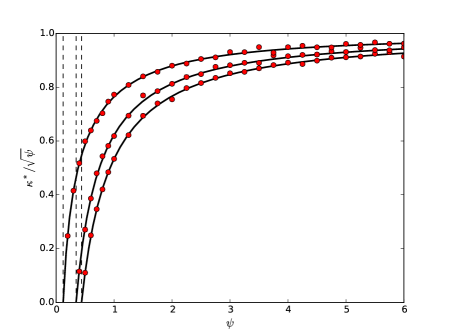
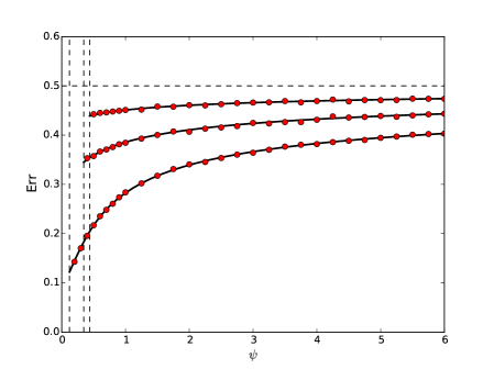
Figure 5: Max-margin linear classification for isotropic well specified data. Left: maximum margin (scaled by $\sqrt{\psi}=\sqrt{p/n}$). Right: test error. Labels are generated using the logistic function $f(x)=(1+e^{-\beta x})^{-1}$ with $\beta=1,2,8$ (from bottom to top on the left, and from top to bottom on the right). Vertical dashed lines correspond to the interpolation threshold $\psi^{*}$, and continuous lines to the analytical predictions of Corollary L.1. Symbols are empirical results for the max-margin (left) and prediction error (right). Here $p=800$ and we vary $n=p/\psi$, averaging results over $20$ instances. Error bars (barely visible) report standard errors on the empirical means of $20$ instances.

We begin by considering the simplest case, namely isotropic covariates ${\boldsymbol{x}}_{i}\sim\mathsf{N}({\boldsymbol{0}},{\boldsymbol{I}}_{p})$, (i.e ${\boldsymbol{\Sigma}}_{n}={\boldsymbol{I}}_{p}$). In this case, by rotational invariance, the margin and prediction error do not depend on the vector ${\boldsymbol{\theta}}_{*,n}$ which has unit norm. Figure 5 report the results of numerical experiments with $p=800$ and various values of $n$. We observe that the classification error decreases as $n$ increase, i.e. as $\psi$ decreases, until it crosses a threshold below which the data is no longer separable.

In order to state our characterization of the maximum margin and prediction error, we introduce the function $F_{\kappa}:\mathbb{R}\times\mathbb{R}_{+}\to\mathbb{R}_{+}$ (for $\kappa\in\mathbb{R}$):

$$F_{\kappa}(c_{1},c_{2})=\left(\mathbb{E}\left[(\kappa-c_{1}YG-c_{2}Z)_{+}^{2}\right]\right)^{1/2}\leavevmode\nobreak\ \leavevmode\nobreak\ \text{where}\leavevmode\nobreak\ \begin{cases}Z\perp(Y,G)\,,\\ Z\sim\mathsf{N}(0,1),G\sim\mathsf{N}(0,1)\,,\\ \mathbb{P}(Y=+1\mid G)=f(G)\,,\\ \mathbb{P}(Y=-1\mid G)=1-f(G)\,.\end{cases}$$ (L.1)

The next corollary is an immediate consequence of our main result, Theorem 3.

Corollary L.1.

Consider the isotropic model, and let $f$ satisfy Assumption 3. Then the following hold:

1. The maximum margin $\kappa_{n}({\boldsymbol{y}},{\boldsymbol{X}})$ converges almost surely to a strictly positive limit if and only if $\psi>\psi^{*}_{\mbox{\tiny\rm iso}}$, where the interpolation threshold is given by

   $$\psi^{*}_{\mbox{\tiny\rm iso}}=\min_{c\geq 0}F_{0}(c,1)^{2}\,.$$ (L.2)

2. For any $\psi>\psi^{*}_{\mbox{\tiny\rm iso}}$ the asymptotic maximum margin is given by $\lim_{n\to\infty}\kappa^{*}_{n}({\boldsymbol{y}},{\boldsymbol{X}})\to\kappa^{*}_{\mbox{\tiny\rm iso}}(\psi)$, where

   $$\kappa^{*}_{\mbox{\tiny\rm iso}}(\psi)=\inf\Big{\{}\,\kappa\geq 0:\;\;F_{\kappa}(c,\sqrt{1-c^{2}})-\sqrt{\psi(1-c^{2})}>0\;\;\;\;\forall c\in[0,1]\Big{\}}\,.$$ (L.3)

3. The asymptotic prediction error is given by $\lim_{n\to\infty}{\rm Err}_{n}({\boldsymbol{y}},{\boldsymbol{X}})={\rm Err}^{*}_{\mbox{\tiny\rm iso}}(\psi)$, where

   $${\rm Err}^{*}_{\mbox{\tiny\rm iso}}(\psi) =\mathbb{P}\Big{(}c^{*}_{\mbox{\tiny\rm iso}}(\psi)YG+\sqrt{1-c^{*}_{\mbox{\tiny\rm iso}}(\psi)^{2}}\,Z\leq 0\Big{)}\,,$$ (L.4)

   $$c^{*}_{\mbox{\tiny\rm iso}}(\psi) \equiv\arg\min_{c\in[0,1]}\,\Big{\{}F_{\kappa=\kappa^{*}_{\mbox{\tiny\rm iso}}}(c,\sqrt{1-c^{2}})-\sqrt{\psi(1-c^{2})}\Big{\}}\,.$$ (L.5)

   (Here expectation is taken with respect to the random variables $(G,Y,Z)$ with joint distribution defined in Eq. (L.1).)

In Figure 6 we compare the theoretical prediction for the maximum margin and test error given in the last corollary with the numerical results: the agreement is excellent. Our analytical predictions confirm the observation made above: the error is monotone increasing in $\psi$, for $\psi>\psi^{*}$. It is possible to show that ${\rm Err}^{*}_{\mbox{\tiny\rm iso}}(\psi)\to 1/2$ as $\psi\uparrow\infty$, while ${\rm Err}^{*}_{\mbox{\tiny\rm iso}}(\psi)\to{\rm Err}^{*}_{\mbox{\tiny\rm iso}}(\psi^{*})$ as $\psi\downarrow\psi^{*}$, where (in general) ${\rm Err}^{*}_{\mbox{\tiny\rm iso}}(\psi^{*})\in(0,1/2)$.

Notice that this behavior is different from the one observed for min-norm least squares [BHX19, HMRT22], under isotropic covariates for a similarly well-specified model. In that case, at small signal-to-noise ratio (SNR), the error is monotone decreasing for $\psi>\psi^{*}$, while at high SNR it is monotone decreasing in an interval $\psi\in(\psi^{*},\psi_{\min})$, and increasing for $\psi>\psi_{\min}$. This different behavior can be explained, at least in part, by the observation that the square loss is unbounded and diverges (for min-norm least squares) at the interpolation threshold. Hence it is necessarily decreasing right above that threshold. In contrast, since the classification error is bounded, it can be monotone increasing with the overparametrization ratio $\psi=p/n$.

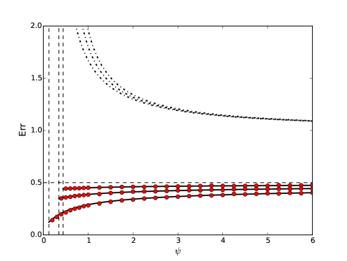
Figure 6: Isotropic well-specified model: comparing margin-based bounds and actual test error. In the lower part of the plot, analytical predictions (continuous lines) and numerical simulations (circles) for the test error: same data as in Figure 5. Dot-dashed lines are margin-based estimates of the test error $\sqrt{\psi}/\kappa^{*}(\psi)$ (see text).

The maximum margin $\kappa^{*}_{\mbox{\tiny\rm iso}}(\psi)$ is also monotone increasing with $\psi$, with $\kappa^{*}_{\mbox{\tiny\rm iso}}(\psi)\downarrow 0$ as $\psi\downarrow\psi^{*}$, and $\kappa^{*}_{\mbox{\tiny\rm iso}}(\psi)/\sqrt{\psi}\to 1$ as $\psi\to\infty$. Notice that the relation between margin and classification error is somewhat counterintuitive. On the basis of classical margin theory [SSBD14], one would expect that the test error increases when the margin decreases. The opposite happens in Fig. 5: as $\psi$ decreases both the error and the margin decrease. The explanation to this counterintuitive phenomenon is related to the fact that, in the present regime, the margin does not concentrate near its population value (and is not separable in this case).

In order to further clarify this phenomenon, in Figure 6 we compare the actual test error (both numerical simulations, and the predictions of Corollary L.1), with a margin-based bound from [SSBD14, Theorem 26.14]. The latter implies, with our notations,

$${\rm Err}_{n}({\boldsymbol{y}},{\boldsymbol{X}})\leq\frac{4r\sqrt{\psi}}{\kappa^{*}(\psi)}+o_{n}(1)\,,\;\;\;\;\;r^{2}\equiv\int x\,\mu({\rm d}x,{\rm d}w)\,.$$ (L.6)

Here $r$ is the typical (normalized) radius of the feature vectors, namely the asymptotic value of $r_{n}^{2}=\mathbb{E}\|{\boldsymbol{x}}_{1}\|^{2}/p$ (in the present case, $r=1$). Even discarding the factor $4$ (which we do in Figure 6), this upper bound has the wrong qualitative dependence on $\psi$ and is never non-trivial in the present setting (never smaller than 1).

We conclude that the isotropic well-specified data distribution does not capture the benefits of overparametrization discussed in the introduction. This is not unexpected: as $p/n$ increases in this setting we are increasing the complexity of the model, but also the complexity of the target function.

L.2 Isotropic misspecified models

Assuming the model to be well specified can be unrealistic. In this section we keep considering isotropic covariates, but introduce a simple misspecification structure to capture the approximation benefits of adding more covariates.

We assume that label $y_{i}$ depend on a potentially infinitely dimensional feature vector ${\boldsymbol{z}}_{i}\in\mathbb{R}^{\infty}$, ${\boldsymbol{z}}_{i}\sim\mathsf{N}(0,{\boldsymbol{I}}_{\infty})$, via

$$\mathbb{P}\big{(}y_{i}=+1\big{|}{\boldsymbol{z}}_{i}\big{)}=f_{0}(\langle{\boldsymbol{\beta}}_{*},{\boldsymbol{z}}_{i}\rangle)\,.$$ (L.7)

Note that this makes mathematical sense as long as ${\boldsymbol{\beta}}_{*}\in\ell_{2}$. Without loss of generality, we can assume $\|{\boldsymbol{\beta}}_{*}\|_{2}=1$. We learn a max-margin classifier over the first $p$ features. Namely, we write ${\boldsymbol{z}}_{i}=({\boldsymbol{x}}_{i},\tilde{\boldsymbol{z}}_{i})$ where ${\boldsymbol{x}}_{i}\in\mathbb{R}^{p}$ contains the first $p$ coordinates of ${\boldsymbol{z}}_{i}$, and $\tilde{\boldsymbol{z}}_{i}$ contains the other coordinates. We then apply max-margin classification to data $\{(y_{i},{\boldsymbol{x}}_{i})\}_{i\leq n}$. Given a vector ${\boldsymbol{v}}\in\mathbb{R}^{\infty}$, we write ${\boldsymbol{\Pi}}_{\leq\ell}{\boldsymbol{v}}$ for the $\ell$-dimensional vector formed by the first $\ell$ entries of ${\boldsymbol{v}}$.

A

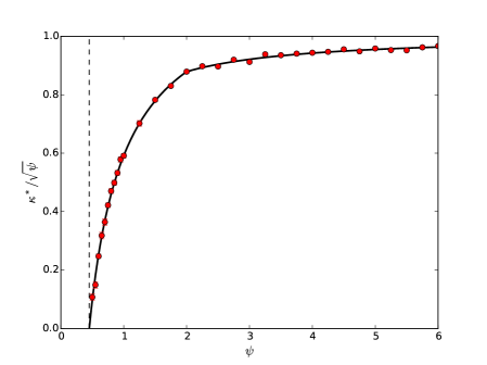
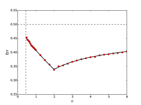
Figure 7: Isotropic miss-specified model. Left: maximum margin (scaled by $\sqrt{\psi}=\sqrt{p/n}$). Right: test error. Labels are generated according to Eq. (L.7), with $f_{0}(x)=(1+e^{-\beta x})^{-1}$, with $\beta=8$. The vertical dashed line corresponds to the interpolation threshold $\psi^{*}_{\mbox{\tiny\rm miss}}$, and the continuous line to the analytical prediction from Corollary L.2. Symbols are empirical results for the prediction error, for $n=400$, $p_{0}=800$ and varying $p=n\psi$, averaged over $20$ instances. Error bars (barely visible) report standard errors on the empirical means of $20$ instances.

This setting can be reduced to the one in the previous section (isotropic well-specified model), whereby labels are assigned according to Eq. (1.6), with $f(x)=\mathbb{E}\{f_{0}(\sqrt{\gamma_{n}}x+\sqrt{1-\gamma_{n}}G^{\prime})\}$ with $G^{\prime}\sim\mathsf{N}(0,1)$ and $\gamma_{n}=\|{\boldsymbol{\Pi}}_{\leq p}{\boldsymbol{\beta}}_{*,n}\|_{2}$. Further ${\boldsymbol{\theta}}_{*,n}={\boldsymbol{\Pi}}_{\leq p}{\boldsymbol{\beta}}_{*,n}/\gamma_{n}$. In words, those features that are not included in the model, and that correspond to non-zero entries in ${\boldsymbol{\beta}}_{*,n}$, act as additional noise in the labels. As more and more features are added to the model, the corresponding noise variance $(1-\gamma_{n})$ decreases.

In order to state the asymptotic characterization of the max margin classifier, we modify the function of Eq. (L.1) as follows

$$F_{\kappa,\gamma}(c_{1},c_{2})=\left(\mathbb{E}\left[(\kappa-c_{1}Y_{\gamma}G-c_{2}Z)_{+}^{2}\right]\right)^{1/2}\leavevmode\nobreak\ \leavevmode\nobreak\ \text{where}\leavevmode\nobreak\ \begin{cases}Z\perp(Y,G)\,,\\ \mathbb{P}(Y_{\gamma}=+1\mid G)=\mathbb{E}[f_{0}(\sqrt{\gamma}G+\sqrt{1-\gamma}G^{\prime})|G]\,,\\ \mathbb{P}(Y_{\gamma}=-1\mid G)=1-\mathbb{E}[f_{0}(\sqrt{\gamma}G+\sqrt{1-\gamma}G^{\prime})|G]\,,\\ Z,G,G^{\prime}\sim_{iid}\mathsf{N}(0,1)\,.\end{cases}$$ (L.8)

Corollary L.2.

Consider the misspecified isotropic model, and let $f_{0}$ satisfy Assumption 3. Further assume ${\boldsymbol{\beta}}_{*,n}\in\mathbb{R}^{\infty}$ to be such that $\|{\boldsymbol{\beta}}_{*,n}\|_{2}=1$ and $\|{\boldsymbol{\Pi}}_{\leq p(n)}{\boldsymbol{\beta}}_{*,n}\|^{2}_{2}\to\gamma(\psi)$ as $n\to\infty$. For any $\psi>0$, define

$$\kappa^{*}_{\mbox{\tiny\rm miss}}(\psi)=\inf\Big{\{}\,\kappa\geq 0:\;\;F_{\kappa,\gamma(\psi)}(c,\sqrt{1-c^{2}})-\sqrt{\psi(1-c^{2})}>0\;\;\;\;\forall c\in[0,1]\Big{\}}\,.$$ (L.9)

1. The maximum margin $\kappa^{*}_{n}({\boldsymbol{y}},{\boldsymbol{X}})$ converges almost surely to a strictly positive limit if and only if $\psi>\psi^{*}_{\mbox{\tiny\rm miss}}\equiv\inf\{\psi>0:\;\kappa^{*}_{\mbox{\tiny\rm miss}}(\psi)>0\}$.

2. For $\psi>\psi^{*}_{\mbox{\tiny\rm miss}}$, the asymptotic max-margin is given by $\lim_{n\to\infty}\kappa^{*}_{n}({\boldsymbol{y}},{\boldsymbol{X}})\to\kappa^{*}_{\mbox{\tiny\rm miss}}(\psi)$.

3. The asymptotic prediction error is given by $\lim_{n\to\infty}{\rm Err}_{n}({\boldsymbol{y}},{\boldsymbol{X}})={\rm Err}^{*}_{\mbox{\tiny\rm miss}}(\psi)$, where

   $${\rm Err}^{*}_{\mbox{\tiny\rm miss}}(\psi) =\mathbb{P}\Big{(}c^{*}_{\mbox{\tiny\rm miss}}(\psi)Y_{\gamma(\psi)}G+\sqrt{1-c^{*}_{\mbox{\tiny\rm miss}}(\psi)^{2}}\,Z\leq 0\Big{)}\,,$$ (L.10)

   $$c^{*}_{\mbox{\tiny\rm miss}}(\psi) \equiv\arg\min_{c\in[0,1]}\,\Big{\{}F_{\kappa=\kappa^{*}_{\mbox{\tiny\rm miss}}(\psi),\gamma(\psi)}(c,\sqrt{1-c^{2}})-\sqrt{\psi(1-c^{2})}\Big{\}}\,.$$ (L.11)

Note that the misspecified model has in important conceptual advantage over the well specified one: the data distribution (L.7) is independent of the number of features

In Figure 7 we consider a misspecified problem in which ${\boldsymbol{\beta}}_{*,n}$ puts equal asymptotically weight over the first $p_{0}$ features, where $p_{0}/n\to\psi_{0}\in(0,\infty)$. Explicitly, we assume $\beta_{*,i}\in\{+1/\sqrt{p_{0}},-1/\sqrt{p_{0}}\}$ for $i\leq p_{0}$, and $\beta_{*,i}=0$ for $i>p_{0}$. This results in $\gamma(\psi)=\psi/\psi_{0}$ if $\psi\leq\psi_{0}$ and $\gamma(\psi)=1$ for $\psi>\psi_{0}$. Note that the same limiting function $\gamma(\psi)$ is obtained for other choices of the vector ${\boldsymbol{\beta}}_{*},n$. For instance, if ${\boldsymbol{\beta}}_{*}$ is a uniformly random vector drawn independent for each $n$, with unit norm and support on $\{1,\dots,p_{0}\}$, the assumptions of Corollary L.2 are satisfied again, with $\gamma(\psi)=\min(\psi/\psi_{0},1)$ as before.

In this example the test error decreases in the overparametrized regime for $\psi^{*}_{\mbox{\tiny\rm miss}}<\psi<\psi_{0}$, and then increases again for $\psi_{0}<\psi$. As explained above, adding more features reduces the approximation error, and hence results in smaller test error. A similar behavior was observed in [HMRT22] for the case of min-norm least squares regression. Notice that the maximum margin is monotone increasing in $\psi$, with $\kappa^{*}(\psi)/\sqrt{\psi}<1$. Further, since $\kappa^{*}(\psi)/\sqrt{\psi}<1$, the classical margin-based bound of Eq. (L.6) is always larger than one. As for the well-specified model, the margin does not seem to capture the behavior of the actual test error.

While the present misspecified data distribution is richer than the well specified distribution of the previous section, it seems too simplistic to capture the benefits of overparametrization in modern machine learning. In particular, the optimum overparametrization ratio $\psi$ is bounded.

References

- [AB09] Martin Anthony and Peter L Bartlett, Neural network learning: Theoretical foundations, Cambridge University Press, 2009.
- [ACHL19] Sanjeev Arora, Nadav Cohen, Wei Hu, and Yuping Luo, Implicit regularization in deep matrix factorization, arXiv:1905.13655 (2019).
- [ALMT14] Dennis Amelunxen, Martin Lotz, Michael B McCoy, and Joel A Tropp, Living on the edge: Phase transitions in convex programs with random data, Information and Inference: A Journal of the IMA 3 (2014), no. 3, 224–294.
- [Bar98] Peter L Bartlett, The sample complexity of pattern classification with neural networks: the size of the weights is more important than the size of the network, IEEE Transactions on Information Theory 44 (1998), no. 2, 525–536.
- [BBV06] Maria-Florina Balcan, Avrim Blum, and Santosh Vempala, Kernels as features: On kernels, margins, and low-dimensional mappings, Machine Learning 65 (2006), no. 1, 79–94.
- [BDM+18] Jean Barbier, Mohamad Dia, Nicolas Macris, Florent Krzakala, and Lenka Zdeborová, Rank-one matrix estimation: analysis of algorithmic and information theoretic limits by the spatial coupling method, arXiv:1812.02537 (2018).
- [BHM18] Mikhail Belkin, Daniel J Hsu, and Partha Mitra, Overfitting or perfect fitting? risk bounds for classification and regression rules that interpolate, Advances in Neural Information Processing Systems, 2018, pp. 2300–2311.
- [BHMM19] Mikhail Belkin, Daniel Hsu, Siyuan Ma, and Soumik Mandal, Reconciling modern machine-learning practice and the classical bias–variance trade-off, Proceedings of the National Academy of Sciences 116 (2019), no. 32, 15849–15854.
- [BHX19] Mikhail Belkin, Daniel Hsu, and Ji Xu, Two models of double descent for weak features, arXiv:1903.07571, 2019.
- [BKM+19] Jean Barbier, Florent Krzakala, Nicolas Macris, Léo Miolane, and Lenka Zdeborová, Optimal errors and phase transitions in high-dimensional generalized linear models, Proceedings of the National Academy of Sciences 116 (2019), no. 12, 5451–5460.
- [BLLT20] Peter L Bartlett, Philip M Long, Gábor Lugosi, and Alexander Tsigler, Benign overfitting in linear regression, Proceedings of the National Academy of Sciences 117 (2020), no. 48, 30063–30070.
- [BLM15] Mohsen Bayati, Marc Lelarge, and Andrea Montanari, Universality in polytope phase transitions and message passing algorithms, The Annals of Applied Probability 25 (2015), no. 2, 753–822.
- [BM02] Peter L Bartlett and Shahar Mendelson, Rademacher and gaussian complexities: Risk bounds and structural results, Journal of Machine Learning Research 3 (2002), no. Nov, 463–482.
- [BM11] Mohsen Bayati and Andrea Montanari, The dynamics of message passing on dense graphs, with applications to compressed sensing, IEEE Trans. on Inform. Theory 57 (2011), 764–785.
- [BM12] , The LASSO risk for gaussian matrices, IEEE Trans. on Inform. Theory 58 (2012), 1997–2017.
- [BM19] Jean Barbier and Nicolas Macris, The adaptive interpolation method: a simple scheme to prove replica formulas in bayesian inference, Probability Theory and Related Fields 174 (2019), no. 3-4, 1133–1185.
- [BMM18] Mikhail Belkin, Siyuan Ma, and Soumik Mandal, To understand deep learning we need to understand kernel learning, arXiv:1802.01396, 2018.
- [BS10] Z. Bai and J. Silverstein, Spectral Analysis of Large Dimensional Random Matrices, Springer, 2010.
- [BVDG11] Peter Bühlmann and Sara Van De Geer, Statistics for high-dimensional data: methods, theory and applications, Springer Science & Business Media, 2011.
- [CB18] Lenaic Chizat and Francis Bach, A note on lazy training in supervised differentiable programming, arXiv:1812.07956 (2018).
- [CL21] Niladri S Chatterji and Philip M Long, Finite-sample analysis of interpolating linear classifiers in the overparameterized regime, The Journal of Machine Learning Research 22 (2021), no. 1, 5721–5750.
- [Cov65] Thomas M Cover, Geometrical and statistical properties of systems of linear inequalities with applications in pattern recognition, IEEE Transactions on Electronic Computers (1965), no. 3, 326–334.
- [CRPW12] V. Chandrasekaran, B. Recht, P. A. Parrilo, and A.S. Willsky, The convex geometry of linear inverse problems, Foundations of Computational Mathematics 12 (2012), 805–849.
- [CS13] Xiuyuan Cheng and Amit Singer, The spectrum of random inner-product kernel matrices, Random Matrices: Theory and Applications 2 (2013), no. 04, 1350010.
- [CS18] Emmanuel J Candès and Pragya Sur, The phase transition for the existence of the maximum likelihood estimate in high-dimensional logistic regression, arXiv:1804.09753 (2018).
- [DAM16] Yash Deshpande, Emmanuel Abbe, and Andrea Montanari, Asymptotic mutual information for the balanced binary stochastic block model, Information and Inference: A Journal of the IMA 6 (2016), no. 2, 125–170.
- [DJM13] David L Donoho, Iain Johnstone, and Andrea Montanari, Accurate prediction of phase transitions in compressed sensing via a connection to minimax denoising, IEEE transactions on information theory 59 (2013), no. 6, 3396–3433.
- [DKT22] Zeyu Deng, Abla Kammoun, and Christos Thrampoulidis, A model of double descent for high-dimensional binary linear classification, Information and Inference: A Journal of the IMA 11 (2022), no. 2, 435–495.
- [DM16] David Donoho and Andrea Montanari, High dimensional robust m-estimation: Asymptotic variance via approximate message passing, Probability Theory and Related Fields 166 (2016), no. 3-4, 935–969.
- [DZPS18] Simon S Du, Xiyu Zhai, Barnabas Poczos, and Aarti Singh, Gradient descent provably optimizes over-parameterized neural networks, arXiv:1810.02054 (2018).
- [EK18] Noureddine El Karoui, On the impact of predictor geometry on the performance on high-dimensional ridge-regularized generalized robust regression estimators, Probability Theory and Related Fields 170 (2018), no. 1-2, 95–175.
- [EKBB+13] Noureddine El Karoui, Derek Bean, Peter J Bickel, Chinghway Lim, and Bin Yu, On robust regression with high-dimensional predictors, Proceedings of the National Academy of Sciences 110 (2013), no. 36, 14557–14562.
- [EVdB01] Andreas Engel and Christian Van den Broeck, Statistical mechanics of learning, Cambridge University Press, 2001.
- [FCB22] Spencer Frei, Niladri S Chatterji, and Peter Bartlett, Benign overfitting without linearity: Neural network classifiers trained by gradient descent for noisy linear data, Conference on Learning Theory, PMLR, 2022, pp. 2668–2703.
- [FM19] Zhou Fan and Andrea Montanari, The spectral norm of random inner-product kernel matrices, Probability Theory and Related Fields 173 (2019), no. 1-2, 27–85.
- [FVBS23] Spencer Frei, Gal Vardi, Peter L Bartlett, and Nathan Srebro, Benign overfitting in linear classifiers and leaky relu networks from kkt conditions for margin maximization, arXiv:2303.01462 (2023).
- [Gar88] Elizabeth Gardner, The space of interactions in neural network models, Journal of physics A: Mathematical and general 21 (1988), no. 1, 257.
- [GJS+19] Mario Geiger, Arthur Jacot, Stefano Spigler, Franck Gabriel, Levent Sagun, Stéphane d’Ascoli, Giulio Biroli, Clément Hongler, and Matthieu Wyart, Scaling description of generalization with number of parameters in deep learning, arXiv:1901.01608 (2019).
- [GLK+20] Federica Gerace, Bruno Loureiro, Florent Krzakala, Marc Mézard, and Lenka Zdeborová, Generalisation error in learning with random features and the hidden manifold model, International Conference on Machine Learning, PMLR, 2020, pp. 3452–3462.
- [GLSS18a] Suriya Gunasekar, Jason Lee, Daniel Soudry, and Nathan Srebro, Characterizing implicit bias in terms of optimization geometry, arXiv:1802.08246 (2018).
- [GLSS18b] Suriya Gunasekar, Jason D Lee, Daniel Soudry, and Nati Srebro, Implicit bias of gradient descent on linear convolutional networks, Advances in Neural Information Processing Systems, 2018, pp. 9461–9471.
- [GMKZ20] Sebastian Goldt, Marc Mezard, Florent Krzakala, and Lenka Zdeborová, Modelling the influence of data structure on learning in neural networks: the hidden manifold model.
- [Gor88] Yehoram Gordon, On Milman’s inequality and random subspaces which escape through a mesh in , Geometric Aspects of Functional Analysis, Springer, 1988, pp. 84–106.
- [HL22] Hong Hu and Yue M Lu, Universality laws for high-dimensional learning with random features, IEEE Transactions on Information Theory (2022).
- [HMRT22] Trevor Hastie, Andrea Montanari, Saharon Rosset, and Ryan J Tibshirani, Surprises in high-dimensional ridgeless least squares interpolation, The Annals of Statistics 50 (2022), no. 2, 949–986.
- [HSS08] T Hofmann, B Schölkopf, and AJ Smola, Kernel methods in machine learning, The Annals of Statistics 36 (2008), no. 3, 1171–1220.
- [HUL13] Jean-Baptiste Hiriart-Urruty and Claude Lemaréchal, Convex analysis and minimization algorithms i: Fundamentals, vol. 305, Springer science & business media, 2013.
- [JGH18] Arthur Jacot, Franck Gabriel, and Clément Hongler, Neural tangent kernel: Convergence and generalization in neural networks, Advances in Neural Information Processing Systems, 2018, pp. 8571–8580.
- [JS22] Adel Javanmard and Mahdi Soltanolkotabi, Precise statistical analysis of classification accuracies for adversarial training, The Annals of Statistics 50 (2022), no. 4, 2127–2156.
- [Kol11] Vladimir Koltchinskii, Oracle inequalities in empirical risk minimization and sparse recovery problems, vol. 2033, Springer Science & Business Media, 2011, Ecole d’Eté de Probabilités de Saint-Flour XXXVIII-2008.
- [KP02] Vladimir Koltchinskii and Dmitry Panchenko, Empirical margin distributions and bounding the generalization error of combined classifiers, The Annals of Statistics 30 (2002), no. 1, 1–50.
- [KPOT21] Ganesh Ramachandra Kini, Orestis Paraskevas, Samet Oymak, and Christos Thrampoulidis, Label-imbalanced and group-sensitive classification under overparameterization, Advances in Neural Information Processing Systems 34 (2021), 18970–18983.
- [KST09] Sham M Kakade, Karthik Sridharan, and Ambuj Tewari, On the complexity of linear prediction: Risk bounds, margin bounds, and regularization, Advances in neural information processing systems, 2009, pp. 793–800.
- [KT20] Ganesh Ramachandra Kini and Christos Thrampoulidis, Analytic study of double descent in binary classification: The impact of loss, 2020 IEEE International Symposium on Information Theory (ISIT), IEEE, 2020, pp. 2527–2532.
- [KZSS21] Frederic Koehler, Lijia Zhou, Danica J Sutherland, and Nathan Srebro, Uniform convergence of interpolators: Gaussian width, norm bounds and benign overfitting, Advances in Neural Information Processing Systems 34 (2021), 20657–20668.
- [LM19] Marc Lelarge and Léo Miolane, Fundamental limits of symmetric low-rank matrix estimation, Probability Theory and Related Fields 173 (2019), no. 3-4, 859–929.
- [LMZ17] Yuanzhi Li, Tengyu Ma, and Hongyang Zhang, Algorithmic regularization in over-parameterized matrix sensing and neural networks with quadratic activations, arXiv:1712.09203 (2017).
- [LR20] Tengyuan Liang and Alexander Rakhlin, Just interpolate: Kernel “ridgeless” regression can generalize, The Annals of Statistics 48 (2020), no. 3, 1329–1347.
- [LS22] Tengyuan Liang and Pragya Sur, A precise high-dimensional asymptotic theory for boosting and minimum--norm interpolated classifiers, The Annals of Statistics 50 (2022), no. 3, 1669–1695.
- [MM09] Marc Mézard and Andrea Montanari, Information, Physics and Computation, Oxford, 2009.
- [MM18] Léo Miolane and Andrea Montanari, The distribution of the lasso: Uniform control over sparse balls and adaptive parameter tuning, arXiv:1811.01212 (2018).
- [MM19] Song Mei and Andrea Montanari, The generalization error of random features regression: Precise asymptotics and double descent curve, arXiv:1908.05355 (2019).
- [MM22] , The generalization error of random features regression: Precise asymptotics and the double descent curve, Communications on Pure and Applied Mathematics 75 (2022), no. 4, 667–766.
- [MNS+21] Vidya Muthukumar, Adhyyan Narang, Vignesh Subramanian, Mikhail Belkin, Daniel Hsu, and Anant Sahai, Classification vs regression in overparameterized regimes: Does the loss function matter?, Journal of Machine Learning Research 22 (2021), no. 222, 1–69.
- [Mon18] Andrea Montanari, Mean field asymptotics in high-dimensional statistics: From exact results to efficient algorithms, Proceedings of the International Congress of Mathematicians, World Scientific, 2018, pp. 2957–2980.
- [MPV87] Marc Mézard, Giorgio Parisi, and Miguel A. Virasoro, Spin glass theory and beyond, World Scientific, 1987.
- [MR+23] Andrea Montanari, , Feng Ruan, Basil N Saeed, and Youngtak Sohn, Universality of max-margin classification, 2023, In preparation.
- [MS22] Andrea Montanari and Basil N Saeed, Universality of empirical risk minimization, Conference on Learning Theory, PMLR, 2022, pp. 4310–4312.
- [MVS19] Vidya Muthukumar, Kailas Vodrahalli, and Anant Sahai, Harmless interpolation of noisy data in regression, arXiv:1903.09139 (2019).
- [MZ22] Andrea Montanari and Yiqiao Zhong, The interpolation phase transition in neural networks: Memorization and generalization under lazy training, The Annals of Statistics 50 (2022), no. 5, 2816–2847.
- [NBMS17] Behnam Neyshabur, Srinadh Bhojanapalli, David McAllester, and Nati Srebro, Exploring generalization in deep learning, Advances in neural information processing systems 30 (2017).
- [Nea96] Radford M Neal, Priors for infinite networks, Bayesian Learning for Neural Networks, Springer, 1996, pp. 29–53.
- [OTH13] Samet Oymak, Christos Thrampoulidis, and Babak Hassibi, The squared-error of generalized lasso: A precise analysis, 2013 51st Annual Allerton Conference on Communication, Control, and Computing (Allerton), 2013, pp. 1002–1009.
- [RR08] Ali Rahimi and Benjamin Recht, Random features for large-scale kernel machines, Advances in Neural Information Processing Systems, 2008, pp. 1177–1184.
- [RZ18] Alexander Rakhlin and Xiyu Zhai, Consistency of interpolation with laplace kernels is a high-dimensional phenomenon, arXiv:1812.11167 (2018).
- [SAH19] Fariborz Salehi, Ehsan Abbasi, and Babak Hassibi, The impact of regularization on high-dimensional logistic regression, arXiv:1906.03761 (2019).
- [SC19] Pragya Sur and Emmanuel J Candès, A modern maximum-likelihood theory for high-dimensional logistic regression, Proceedings of the National Academy of Sciences 116 (2019), no. 29, 14516–14525.
- [SHN+18] Daniel Soudry, Elad Hoffer, Mor Shpigel Nacson, Suriya Gunasekar, and Nathan Srebro, The implicit bias of gradient descent on separable data, The Journal of Machine Learning Research 19 (2018), no. 1, 2822–2878.
- [SSBD14] Shai Shalev-Shwartz and Shai Ben-David, Understanding machine learning: From theory to algorithms, Cambridge University Press, 2014.
- [ST03] Mariya Shcherbina and Brunello Tirozzi, Rigorous solution of the Gardner problem, Communications in Mathematical Physics 234 (2003), no. 3, 383–422.
- [Sto10] Mihailo Stojnic, l1 optimization and its various thresholds in compressed sensing, 2010 IEEE International Conference on Acoustics, Speech and Signal Processing, 2010, pp. 3910–3913.
- [Sto13] , A framework to characterize performance of lasso algorithms, arXiv:1303.7291 (2013).
- [TAH18] Christos Thrampoulidis, Ehsan Abbasi, and Babak Hassibi, Precise error analysis of regularized -estimators in high dimensions, IEEE Transactions on Information Theory 64 (2018), no. 8, 5592–5628.
- [TB20] Alexander Tsigler and Peter L Bartlett, Benign overfitting in ridge regression, arXiv:2009.14286 (2020).
- [TOH15] Christos Thrampoulidis, Samet Oymak, and Babak Hassibi, Regularized linear regression: A precise analysis of the estimation error, Conference on Learning Theory, 2015, pp. 1683–1709.
- [TPT20] Hossein Taheri, Ramtin Pedarsani, and Christos Thrampoulidis, Fundamental limits of ridge-regularized empirical risk minimization in high dimensions, arXiv:2006.08917 (2020).
- [Ver18a] Roman Vershynin, High-dimensional probability: An introduction with applications in data science, vol. 47, Cambridge University Press, 2018.
- [Ver18b] , High-dimensional probability: An introduction with applications in data science, vol. 47, Cambridge University Press, 2018.
- [Vil08] Cédric Villani, Optimal transport: old and new, vol. 338, Springer Science & Business Media, 2008.
- [Wah02] Grace Wahba, Soft and hard classification by reproducing kernel hilbert space methods, Proceedings of the National Academy of Sciences 99 (2002), no. 26, 16524–16530.
- [ZBH+16] Chiyuan Zhang, Samy Bengio, Moritz Hardt, Benjamin Recht, and Oriol Vinyals, Understanding deep learning requires rethinking generalization, arXiv:1611.03530 (2016).
- [ZKS+22] Lijia Zhou, Frederic Koehler, Pragya Sur, Danica J Sutherland, and Nathan Srebro, A non-asymptotic moreau envelope theory for high-dimensional generalized linear models, arXiv:2210.12082 (2022).