Model uncertainty estimation using the expectation maximization algorithm and a particle flow filter

Abstract

Model error covariances play a central role in the performance of data assimilation methods applied to nonlinear state-space models. However, these covariances are largely unknown in most of the applications. A misspecification of the model error covariance has a strong impact on the computation of the posterior probability density function, leading to unreliable estimations and even to a total failure of the assimilation procedure. In this work, we propose the combination of the Expectation-Maximization algorithm (EM) with an efficient particle filter to estimate the model error covariance, using a batch of observations. Based on the EM algorithm principles, the proposed method encompasses two stages: the expectation stage, in which a particle filter is used with the present estimate of the model error covariance as given to find the probability density function that maximizes the likelihood, followed by a maximization stage in which the expectation under the probability density function found in the expectation step is maximized as a function of the elements of the model error covariance. This novel algorithm here presented combines the EM with a fixed point algorithm and does not require a particle smoother to approximate the posterior densities. We demonstrate that the new method accurately and efficiently solves the linear model problem. Furthermore, for the chaotic nonlinear Lorenz-96 model the method is stable even for observation error covariance 10 times larger than the estimated model error covariance matrix, and also that it is successful in high-dimensional situations where the dimension of the estimated matrix is 1600.

Keywords: Particle Filters, State-Space Models, Model error covariance, EM algorithm

1 Introduction

Several research areas in which the object of research is a complex system, such as for instance the atmosphere, the ocean and biological systems, require to estimate the state of the system through partial observational information which is distributed in time. Surrogate models of the system, which represent approximately the time evolution of the variables, are included as a source of information in the state estimation. This has a twofold aim, it regularizes the state estimation at a time and propagates information of the system and its uncertainty to the subsequent times. This estimation problem was called data assimilation in geophysical sciences [6, 16], and this terminology has then been popularized in other areas. The so-called state-space model is composed by two stochastic equations, one represents the evolution of the hidden state variables, henceforth referred as dynamical model, and the other one maps the state of the system into the observations space through an observational model.

The increase of observational data availability, particularly indirect observations, and the increased complexity in surrogate models, introduce nonlinear dependencies in the dynamical and observational models which in turn lead to non-Gaussian statistics. To account for these non-Gaussian statistics in high-dimensional state-space models is essential for the inference and represents one of the major challenges in the area [11, 31, 37]. Gaussianity-based techniques such as all the variants of the Kalman filter and optimization techniques based on maximum a posteriori estimation, also known as variational data assimilation, cannot deal with strongly non-Gaussian statistics. Monte Carlo techniques are one of the most promising methodologies that can fully consider the non-Gaussian uncertainty in the sequential inference [10, 13, 23]. These techniques aim to represent the state distribution by a set of realizations (referred as particles) of this distribution. Particles are evolved between estimation times by the use of the dynamical model. However, one contention point in these techniques is the particle degeneracy along the time sequence. After a few cycles, most of the particles finish with negligible weights, i.e., their likelihood to the observation is low or null, and only one particle remains with weight 1. This limitation is particularly important in high-dimensional systems. One solution is resampling, however it brings another limitation since only a few particles with large weight remain and therefore the diversity is lost, particularly in experiments which can only afford a small number of particles.

Recently a new framework for particle filters, called particle flow filters, has been proposed [3, 7]. Within this framework, particles are moved from the initial proposed distribution to the posterior distribution using flows that are consistent with Bayes rule. Particle flows potentially avoid the need of resampling since the particles are moved to regions of higher likelihood of the state space. The flow is not unique and requires the solution of an ordinary differential equation under a given regularization. Alternatively, if the Gaussian assumption is taken, the expression for the flow can be derived analytically and the flow is unique and known as Gaussian particle flow. In a recent work, Pulido and vanLeeuwen [21] showed that under the assumption that the flow lies in a reproducing kernel Hilbert space, then it is uniquely determined through a Monte Carlo integration, an interacting particle system. This approach combines Monte Carlo sampling with variational inference. It is shown that this sequential Monte Carlo filter does not require resampling even for long time sequences and can work in relatively high-dimensional systems.

A crucial assumption in particle filters is that the model error is known. The model error uncertainty is included in the evolution of the particles and is essential to account for the prediction uncertainty. This is particularly the case in particle flow filters, in which the sequential prior density is assumed to be known. In practice, model error is not known and it is highly dependent on the surrogate model we are using. The structure of the model error, in terms for example of correlation between variables, is expected to be different if different surrogate models are used. Therefore, there is a current need for the development of model error estimation techniques that may be applied for sequential Monte Carlo filters.

Likelihood-based methods for model error covariance estimation may be broadly classified into two groups: maximum likelihood estimation and Bayesian inference. Maximum likelihood estimation methods have been applied assuming that covariance parameters are deterministic [4, 15, 31, 32]. In this case, non a priori information on the parameters is required. When the gradient of the likelihood can be obtained analytically, Newton-Raphson optimization methods may be applied to maximize the likelihood function. When this is not feasible one of the most popular methods for maximum likelihood estimation is expectation maximization (EM) [8]. One of the reasons of its widespread use is that it is readily applicable. In particular, contrary to Newton-Raphson optimization methods, expectation-maximization does not depend on (optimization) parameters. The second group is a Bayesian approach in which the model error covariance parameters are interpreted as stochastic and the prior distribution of the parameters needs to be given. In this case, some hypotheses on the correlations between state space variables and parameters are required in high-dimensional systems [24]. Some authors [18, 29] assume that the uncertainty in the parameters does not affect the state density, while [25] use the marginalization of the hidden state for the parameter estimation in a hierarchical Bayesian framework.

In this article, we propose a new method based on a maximum likelihood approach to estimate the model error covariance matrix in state-space models. The article is organized as follows. In section 2 we formulate the problem giving a brief overview of particle filters and some details of a recently proposed particle flow filter to be used in the experiments before describing the proposed method to estimate the model error covariance matrix in section 2.3. Further details about its derivation are given in section 5 and section 6. The proposed method is tested on a simple autoregressive linear model and on the Lorenz-96 model with 8 and 40 dimensions. Experiments design, results, and comparison with existing methods are shown in section 3 while in section 4 we present some conclusions.

2 Methodology

2.1 Problem formulation

Consider a state-space model, consisting of a non-linear system and a non-linear observation model, described by

$${\bf{x}}_{k} ={\mathcal{M}}({\bf x}_{k-1})+\mbox{\boldmath$\beta$}_{k}$$ (1)

$${\bf{y}}_{k} ={\mathcal{H}}({\bf{x}}_{k})+\mbox{\boldmath$\epsilon$}_{k}$$ (2)

where ${\bf{x}}_{k}\in\mathbb{R}^{N_{x}}$, called the state vector, is a hidden or latent process, $\{{\bf y}_{k}\}_{k=1}^{K}$ is a time series of observations measured at times $k=1,\ldots,K$ with ${\bf y}_{k}\in\mathbb{R}^{M}$. The maps $\mathcal{M}(.)$ and $\mathcal{H}(.)$ denote the non-linear deterministic dynamical model and the (possibly non linear) observation operator, respectively. The state process is assumed to be a Markov process, whereas the conditional density of the observations ${\bf y}_{k}$ depends only on the current state $\mathbf{x}_{k}$ for $k=1,\ldots,K$. The stochastic term $\mbox{\boldmath$\beta$}_{k}$ accounts for the missing physics in the model and its numerical approximations, whereas $\mbox{\boldmath$\epsilon$}_{k}$ is the observation noise. In this work, we assume that observational and model uncertainty are additive and $\mbox{\boldmath$\beta$}_{k}\sim\mathcal{N}(0,{\bf Q}_{k})$ and $\mbox{\boldmath$\epsilon$}_{k}\sim\mathcal{N}(0,\mathbf{R}_{k})$, where $\mathbf{Q}_{k}$ and $\mathbf{R}_{k}$ belong to the subspace of positive definite matrices in $\mathbb{R}^{N_{x}\times N_{x}}$ and $\mathbb{R}^{M\times M}$, respectively, representing the model error and observation error covariance matrices at time $k$. We denote by $\mbox{\boldmath$\theta$}_{k}\in\mbox{\boldmath$\Theta$}$ the vector of parameters $(\mathbf{Q}_{k},\mathbf{R}_{k})$.

Since $\mathcal{M}$ and $\mathcal{H}$ are surrogate models which approximate the system evolution and the processes that relate the observations with the hidden state, the model error and observational error covariances are expected to be largely unsconstrained physically. Observational errors may be partially constrained from the knowledge of measurement errors, whereas representation errors, arising from the fact that model and observations often represent reality differently, are hard to determine in practice. Therefore, the parameters $\mbox{\boldmath$\theta$}_{k}$ of the state space model are unknown and need to be inferred from the data as well as the hidden state $\mathbf{x}_{k}$. In principle, unknown parameters from the dynamical and observational models may also be included in $\mbox{\boldmath$\theta$}_{k}$ [20]; in this work we consider these parameters are provided.

We assume that the model error covariance $\mathbf{Q}_{k}$ and the observation error covariance $\mathbf{R}_{k}$ vary slowly within $K$-cycles   (the temporal scale of covariance variations is longer that $K$-cycles), that is $\mathbf{Q}_{k}=\mathbf{Q}$, $\mathbf{R}_{k}=\mathbf{R}$, $\forall k=1,\ldots,K$ and propose a method based on a time-batch of observations to estimate the model error covariance $\mathbf{Q}$ for particle filters (PF). The information provided by the observations along the $K$ times, $\mathbf{y}_{1:K}$, where the subindices $1:K$ denote the set $\{{\bf y}_{1},\ldots,{\bf y}_{K}\}$, is considered essential to regularize/constrain the $N_{x}\times N_{x}$ unknowns from $\mathbf{Q}$. The coupling between observations at different times is produced through the dynamical model $\mathcal{M}$.

The method here presented is based on maximum likelihood estimation: given a set of independent observations $\{{\bf{y}}_{k},k=1,\ldots,K\}$ from a probability density function represented by $p({\bf y}_{1:K};\mbox{\boldmath$\theta$})$, a nonlinear dynamical model $\mathcal{M}$ and an observation operator $\mathcal{H}$, we seek to maximize the likelihood of the observations as a function of the statistical parameters $\mathbf{Q}$ given an observation error covariance $\mathbf{R}$ in the presence of a hidden state $\mathbf{x}_{0:K}$.

2.2 Particle filters

State-space models are generally used in sequential data assimilation to estimate or reconstruct the hidden state ${\bf x}_{k}$ given the observations ${\bf y}_{1:K}$. This can be done by computing the filter densities $\{p(\mathbf{x}_{k}|\mathbf{y}_{1:k})\}_{k=1:K}$ or smoother densities $\{p(\mathbf{x}_{k}|\mathbf{y}_{1:s})\}_{k=1:K}$ with $s\geq k$. Having prior knowledge of the initial state ${\bf x}_{0}$, that is, given a prior background probability density function (pdf) $p({\bf x}_{0})$, the posterior pdf of a filter is the probability of the model state at time $k$, given all the available information up to time $k$. In a Markovian system with observations ${\bf y}_{k}$ that are conditionally independent given the state, the filter densities can be computed recursively using Bayes’ rule to obtain the posterior pdf

$$p(\mathbf{x}_{k}|\mathbf{y}_{1:k};\mbox{\boldmath$\theta$})=\frac{p({\bf y}_{k}|{\bf x}_{k};\mbox{\boldmath$\theta$})p({\bf x}_{k}|{\bf y}_{1:k-1};\mbox{\boldmath$\theta$})}{p({\bf y}_{k}|{\bf y}_{1:k-1};\mbox{\boldmath$\theta$})},$$ (3)

where the prior pdf $p({\bf x}_{k}|{\bf y}_{1:k-1};\mbox{\boldmath$\theta$})$ is the forecast or prediction pdf, $p({\bf y}_{k}|{\bf x}_{k};\mbox{\boldmath$\theta$})$ is the observation likelihood defined by the observation model $\mathcal{H}$ and the distribution of the observation error $\mbox{\boldmath$\epsilon$}_{k}$, and $p({\bf y}_{k}|{\bf y}_{1:k-1};\mbox{\boldmath$\theta$})$ is a normalizing factor. Note that we consider here the marginalized posterior pdf, in which the only state variable that is estimated is the current one, considering all the past and the current observations. This assumption is essential when dealing with high-dimensional systems.

When the dynamical and observational models are linear and their errors Gaussian, the filter densities are Gaussian and the state can be computed using Kalman recursive algorithms. However, for nonlinear models and/or nonlinear observational functions it is not possible to get a known distribution or a closed form for these filter pdf’s, and they should be somehow approximated. Classical particle filters [1, 10, 34] are based on sequential importance sampling and resampling algorithms and provide different methods to approximate these pdfs.

The basic idea behind a particle filter is to represent the posterior pdf $p(\mathbf{x}_{k}|\mathbf{y}_{1:k})$ by a set of $N_{p}$ particles $\{x^{(j)}_{k}\}_{j=1:N_{p}}$ with corresponding weights $\{w_{k}^{(j)}\}_{j=1:N_{p}}$ such that $\sum_{j=1}^{N_{p}}w_{k}^{(j)}=1$. That is, at time $k$, $p(\mathbf{x}_{k}|\mathbf{y}_{1:k};\mbox{\boldmath$\theta$})$ is approximated by

$$p(\mathbf{x}_{k}|\mathbf{y}_{1:k};\mbox{\boldmath$\theta$})\doteq\sum_{j=1}^{N_{p}}w_{k}^{(j)}\delta({\bf x}_{k}-{\bf x}_{k}^{(j)})$$ (4)

where $\doteq$ denotes approximation by an ensemble of particles and $\delta(\cdot)$ is the Dirac $\delta$ function.

Initially, a set of $N_{p}$ particles$\{x^{(j)}_{0}\}_{j=1:N_{p}}$ with corresponding weights $\{w_{0}^{(j)}=\frac{1}{N_{p}}\}_{j=1:N_{p}}$ is drawn from the prior pdf $p({\bf x}_{0})$. These particles are sequentially evolved in time using a forecasting, weighting and resampling scheme to obtain $\{x^{(j)}_{k}\}_{j=1:N_{p}}$ and $\{w_{k}^{(j)}\}_{j=1:N_{p}}$ at each time step $k$. Different PFs were proposed depending on the resampling, forecasting or weighting approaches taken [1, 21, 39].

2.2.1 Variational mapping particle filter

The variational mapping particle filter,VMPF, is a particle filter which is based on optimization and Monte Carlo sampling. The particles are moved deterministically via a sequence of maps, based on the optimal transport principle. The maps seek to minimize the Kullback-Leibler divergence (KLD) between the target density, i.e. the posterior density $p(\mathbf{x}_{k}|\mathbf{y}_{1:k})$, and an intermediate density $q(\mathbf{x}_{k})$, that is the density represented through the sample, the set of particles, at a given cycle $k$. At the $i$-th optimization iteration, the KLD is given by

$$\mathcal{D}_{KL}(q_{k,i}(\mathbf{x}_{k})\rVert p(\mathbf{x}_{k}|\mathbf{y}_{1:k}))=\int q_{i}(\mathbf{x}_{k})\log\frac{q_{k,i}(\mathbf{x}_{k})}{p(\mathbf{x}_{k}|\mathbf{y}_{1:k})}\mathrm{d}\mathbf{x}_{k},$$ (5)

where the $q_{i}(\mathbf{x}_{k})$ is represented via $N_{p}$ sample points, i.e. particles, $\mathbf{x}^{(1:N_{p})}_{k,i}\sim q_{i}(\mathbf{x}_{k})$.

The density $q_{i}$ is the result of a map, $T_{i}(\mathbf{x}_{k,i-1})=\mathbf{x}_{k,i-1}+\epsilon\mathbf{v}_{i}(\mathbf{x}_{k,i-1})$, which is a small perturbation to the identity map ($\epsilon$ is assumed to be small). This means $q_{i}=T_{i}^{\sharp}q_{i-1}=q_{i-1}(T_{i}^{-1})|\det J(T_{i}^{-1})|$. The maps are assumed to be in a reproducing kernel Hilbert space.

The optimal map that gives the steepest descent direction is shown to be given by

$$\mathbf{v}_{i}(\mathbf{x}_{k,i-1})=-\nabla\mathcal{D}_{KL}(\mathbf{x}_{k})=\mathcal{E}_{x^{\prime}_{k}\sim q}\left[\mathbf{K}(\mathbf{x}^{\prime}_{k},\mathbf{x}_{k})\nabla_{x^{\prime}_{k}}\log p(\mathbf{x}^{\prime}_{k}|y_{1:k})+\nabla_{x^{\prime}}\mathbf{K}(\mathbf{x}^{\prime}_{k},\mathbf{x}_{k})\right],$$ (6)

where $\mathbf{K}$ is a kernel (assumed here to be Gaussian) [21].

Then the optimization is a sequence of (sufficiently smooth) mappings for each particle $(j)$ along the steepest descent direction

$$\mathbf{x}_{k,i}^{(j)}=\mathbf{x}_{k,i-1}^{(j)}-\epsilon\nabla\mathcal{D}_{KL}(\mathbf{x}_{k,i-1}^{(j)}).$$ (7)

If observational and model errors are assumed to be Gaussian, the gradient of the log-posterior density is

$$\nabla_{\mathbf{x}}\log p(\mathbf{x}_{k})=\mathbf{H}^{\top}\mathbf{R}_{k}^{-1}\left(\mathbf{y}_{k}-\mathcal{H}(\mathbf{x}_{k})\right)-\mathbf{Q}_{k}^{-1}\left[\mathbf{x}_{k}-\sum_{j=1}^{N_{p}}\mbox{\boldmath$\beta$}_{k-1}^{(j)}\mathcal{M}(\mathbf{x}^{(j)}_{k-1})\right],$$ (8)

where $\mbox{\boldmath$\beta$}_{k-1}^{(j)}\triangleq\frac{w_{k-1}^{(j)}\psi^{(j)}_{\mathbf{Q}_{k}}}{\sum_{m=1}^{N_{p}}w_{k-1}^{(m)}\psi^{(m)}_{\mathbf{Q}_{k}}}$, and $\psi^{(j)}_{\mathbf{Q}_{k}}=\exp(-\rVert\mathbf{x}_{k}-\mathbf{x}_{k}^{(j)}\lVert^{2}_{\mathbf{Q}_{k}})$. They could be interpreted as weights of the forecast states which consider the distance between the particles to the point under consideration. A more detailed description of the VMPF is found in [21]. Recently, a generalization to embed also the observational operator in the RKHS was proposed in [22]

One of the main advantages of the VMPF is that not only it efficiently samples high- dimensional state spaces with a limited number of particles but also it does not suffer from sample impoverishment.

2.3 Parameter estimation

Let us assume that $p(\cdot;\mbox{\boldmath$\theta$})$ is a parametric distribution, with $\mbox{\boldmath$\theta$}\in\mbox{\boldmath$\Theta$}$, the parameter space. Given a set of observations ${\bf y}_{1:K}=\{{\bf{y}}_{k},k=1,\ldots,K\}$ taken along a time interval of length $K$, a maximum likelihood estimation method aims at finding the value of $\theta$ that maximizes the (incomplete) likelihood of the observations,

$$L(\mbox{\boldmath$\theta$})=p({\bf y}_{1:K};\mbox{\boldmath$\theta$})=\int p(\mathbf{x}_{0:K},\mathbf{y}_{1:K};\mbox{\boldmath$\theta$})\mathrm{d}\mathbf{x}_{0:K},$$ (9)

or equivalently, the log-likelihood function

$$l(\mbox{\boldmath$\theta$})=\ln p({\bf y}_{1:K};\mbox{\boldmath$\theta$})=\ln\left(\int p(\mathbf{x}_{0:K},\mathbf{y}_{1:K};\mbox{\boldmath$\theta$})\mathrm{d}\mathbf{x}_{0:K}\right).$$ (10)

The likelihood function eq. 9 can be interpreted as how probable the set of observations $\mathbf{y}_{1:K}$ would be for different choices of $\theta$. An analytic form for the log-likelihood function is not achievable in practice, and the numerical evaluation of eq. 10 may involve high-dimensional integrations, what is intractable. In some situations the optimization task can be accomplished by using numerical optimization routines like Newton-Raphson techniques to solve the nonlinear equations obtained by differentiating the log-likelihood function eq. 10 [4, 14, 20]. However, even in these particular situations, other methods are preferable due to the difficulty of implementing optimization methods and tuning their parameters. Gradient optimization methods may be not stable numerically for certain sets of parameters.

The expectation-maximization (EM) algorithm [8], is a widely used numerical method that aims at maximizing the log-likelihood of the observations as a function of the statistical parameters $\theta$ in the presence of a hidden state $\mathbf{x}_{0:K}$ in successive iterations without the need to evaluate the complete log-likelihood function.

It basically consists in maximizing iteratively an intermediate function defined as

$$\mathcal{G}(\mbox{\boldmath$\theta$}^{\prime},\mbox{\boldmath$\theta$}) \triangleq\mathbb{E}_{\mbox{\boldmath$\theta$}^{\prime}}\left[\ln p(\mathbf{x}_{0:K},\mathbf{y}_{1:K};\mbox{\boldmath$\theta$})\right]$$ (11)

$$=\int\ln p(\mathbf{x}_{0:K},\mathbf{y}_{1:K};\mbox{\boldmath$\theta$})p(\mathbf{x}_{0:K}|\mathbf{y}_{1:K};\mbox{\boldmath$\theta$}^{\prime})\mathrm{d}\mathbf{x}_{0:K}$$ (12)

where $\mbox{\boldmath$\theta$}^{\prime},\mbox{\boldmath$\theta$}\in\mbox{\boldmath$\Theta$}$. This intermediate function $\mathcal{G}$ is, generally, much simpler to maximize than the incomplete log-likelihood defined in eq. 10.

Starting from an initial parameter $\mbox{\boldmath$\theta$}_{0}$, the two steps of the EM algorithm at iteration $s$ can be summarized as:

• Expectation Step (E-Step): Calculate the required densities to compute the intermediate function $\mathcal{G}(\mbox{\boldmath$\theta$}_{s-1},\mbox{\boldmath$\theta$})$ as in eq. 12.

• Maximization Step (M-Step): find $\mbox{\boldmath$\theta$}_{s}=\displaystyle\max_{\mbox{\boldmath$\theta$}\in\mbox{\boldmath$\Theta$}}\mathcal{G}(\mbox{\boldmath$\theta$}_{s-1},\mbox{\boldmath$\theta$})$.

The assumptions of a hidden Markov model and mutually independent observations in eq. 1 allow us to express the joint probability density function $p(\mathbf{x}_{0:K},\mathbf{y}_{1:K};\mbox{\boldmath$\theta$})$ as

$$p(\mathbf{x}_{0:K},\mathbf{y}_{1:K};\mbox{\boldmath$\theta$})=p(\mathbf{x}_{0};\mbox{\boldmath$\theta$})\prod_{k=1}^{K}p(\mathbf{x}_{k}|\mathbf{x}_{k-1};\mbox{\boldmath$\theta$})\prod_{k=1}^{K}p(\mathbf{y}_{k}|\mathbf{x}_{k};\mbox{\boldmath$\theta$}).$$ (13)

To estimate the parameters of the state-space model using the EM algorithm, the expectation of this last pdf under the conditional (smoother) pdf $p(\mathbf{x}_{0:K}|\mathbf{y}_{1:K};\mbox{\boldmath$\theta$}^{\prime})$ must be computed in the E-Step of the algorithm. In the case of a linear Gaussian model this can be accomplished by means of a Kalman smoother [27]. This was further extended to the ensemble Kalman filter in [12, 20].

When the dynamical or observational model are non-linear and therefore the joint density non-Gaussian, the expectation in equation eq. 11 may be intractable and a different approach must be taken. A generally used approach is to approximate the expression in eq. 11 by generating samples of the smoother pdf $p(\mathbf{x}_{0:K}|\mathbf{y}_{1:K};\mbox{\boldmath$\theta$}^{\prime})$ using a particle smoother [2, 15, 19]. However, the use of particle smoothers in data assimilation represents a computational challenge, since they not only tend to degenerate rapidly but also have a poor performance in moderate to high dimensional spaces, particularly if the time sequence is long (large $K$).

The requirement of a particle smoother in the E-Step of the EM algorithm is due to the fact that the likelihood of the observations $p(\mathbf{y}_{1:K};\mbox{\boldmath$\theta$})$ is usually obtained by marginalizing the joint pdf $p(\mathbf{x}_{0:K},\mathbf{y}_{1:K};\mbox{\boldmath$\theta$})$ over the whole state $\mathbf{x}_{0:K}$ (cf. equation eq. 9).

Instead of using this last expression for the likelihood of the observations, and following the notation of [5], the likelihood of the observations (model evidence) can be decomposed as $p(\mathbf{y}_{1:K};\mbox{\boldmath$\theta$})=\prod^{K}_{k=1}p(\mathbf{y}_{k}|\mathbf{y}_{k-1};\mbox{\boldmath$\theta$})$, with the convention $\mathbf{y}_{1:0}=\{\emptyset\}$. Marginalizing this last expression we obtain

$$p(\mathbf{y}_{1:K};\mbox{\boldmath$\theta$}) =\prod^{K}_{k=1}p(\mathbf{y}_{k}|\mathbf{y}_{k-1};\mbox{\boldmath$\theta$})$$

$$=\prod^{K}_{k=1}\int p(\mathbf{y}_{k}|\mathbf{x}_{k};\mbox{\boldmath$\theta$})p(\mathbf{x}_{k}|\mathbf{y}_{1:k-1};\mbox{\boldmath$\theta$})\mathrm{d}\mathbf{x}_{k}$$ (14)

and therefore we can rewrite the logarithm of the incomplete likelihood eq. 9 as

$$l(\mbox{\boldmath$\theta$})=\log p(\mathbf{y}_{1:K};\mbox{\boldmath$\theta$})=\log\prod^{K}_{k=1}\int p(\mathbf{y}_{k}|\mathbf{x}_{k};\mbox{\boldmath$\theta$})p(\mathbf{x}_{k}|\mathbf{y}_{1:k-1};\mbox{\boldmath$\theta$})\mathrm{d}\mathbf{x}_{k}.$$ (15)

Using this last expression instead of the commonly used expression eq. 10, the intermediate function $\mathcal{G}(\mbox{\boldmath$\theta$}^{\prime},\mbox{\boldmath$\theta$})$ of the EM algorithm can be written as

$$\mathcal{G}(\mbox{\boldmath$\theta$}^{\prime},\mbox{\boldmath$\theta$}) =\sum_{k=1}^{K}\int p(\mathbf{x}_{k}|\mathbf{y}_{1:k};\mbox{\boldmath$\theta$}^{\prime})\log\left(\frac{p(\mathbf{y}_{k}|\mathbf{x}_{k};\mbox{\boldmath$\theta$})p(\mathbf{x}_{k}|\mathbf{y}_{1:k-1};\mbox{\boldmath$\theta$})}{p(\mathbf{x}_{k}|\mathbf{y}_{1:k};\mbox{\boldmath$\theta$}^{\prime})}\right)\mathrm{d}\mathbf{x}_{k}$$ (16)

as it is shown in section 5. Note that this last expression for $\mathcal{G}(\mbox{\boldmath$\theta$}^{\prime},\mbox{\boldmath$\theta$})$ is written in terms of filter and forecast pdf’s, while smoother pdf’s are no longer required. As the denominator of eq. 16 does not depend on $\theta$, maximizing $\mathcal{G}(\mbox{\boldmath$\theta$}^{\prime},\mbox{\boldmath$\theta$})$ w.r.t $\theta$ is equivalent to maximizing

$$\mathcal{G}(\mbox{\boldmath$\theta$}^{\prime},\mbox{\boldmath$\theta$}) =\sum_{k=1}^{K}\int p(\mathbf{x}_{k}|\mathbf{y}_{1:k};\mbox{\boldmath$\theta$}^{\prime})\log\left(p(\mathbf{y}_{k}|\mathbf{x}_{k};\mbox{\boldmath$\theta$})p(\mathbf{x}_{k}|\mathbf{y}_{1:k-1};\mbox{\boldmath$\theta$})\right)\mathrm{d}\mathbf{x}_{k}$$ (17)

$$=\sum_{k=1}^{K}\mathcal{E}_{\mbox{\boldmath$\theta$}^{\prime}}\left[\log(p(\mathbf{y}_{k}|\mathbf{x}_{k};\mbox{\boldmath$\theta$})p(\mathbf{x}_{k}|\mathbf{y}_{1:k-1};\mbox{\boldmath$\theta$}))\right].$$ (18)

So far $\theta$ denotes the set comprised by $(\mathbf{Q},\mathbf{R})$, the model error and observation error covariance matrices, respectively. As there is a certain degree of knowledge about the instruments noise and how observations are measured or obtained, $\mathbf{R}$ is usually determined empirically in practice by estimating these noises and the errors between the state and observation space. However, this is far from being an accurate representation of $\mathbf{R}$ and during the last few years a great effort has been dedicated to the study and estimation of the observation error covariance matrix, and many works have been published on these topics ([28, 32, 33, 35] and references therein). Some of these works focus on studying the most plausible structure for $\mathbf{R}$ given the nature of how observations were measured taking into account correlations between observation errors whilst some others just propose a fixed structure for $\mathbf{R}$ and a methodology to estimate it. What these different approaches have in common is that they assume that the model error covariance matrix is already given, or known. The model error covariance matrix $\mathbf{Q}$ is, perhaps, the most difficult one to estimate or determine, since it accounts for the model inaccuracies and deficiencies in representing the missing underlying physics, the errors in parameterizations, the unresolved and smaller scales and the numerical schemes used. Some works have been devoted to the joint estimation of $(\mathbf{Q},\mathbf{R})$ and an up to date and detailed review of these techniques is presented in [30].

The main purpose of this work is to provide a method to estimate $\mathbf{Q}$, the covariance matrix of the model error $\beta$. Assuming that $\mathbf{R}$ is known, replacing $\mbox{\boldmath$\theta$}=\mathbf{Q}$ and having in mind that by hypothesis the density $p(\mathbf{y}_{k}|\mathbf{x}_{k};\mathbf{Q})$ is assumed to be independent of $\mathbf{Q}$, then starting from an initial guess $\mathbf{Q}_{0}$, the two steps of the EM algorithm at iteration $s$ can be summarized as:

• Expectation Step (E-Step): Calculate the required densities to compute the intermediate function

  $$\mathcal{G}(\mathbf{Q}_{s-1},\mathbf{Q})=\sum_{k=1}^{K}\mathcal{E}_{\mathbf{Q}_{s-1}}\left[\log(p(\mathbf{x}_{k}|\mathbf{y}_{1:k-1};\mathbf{Q}))\right].$$ (19)

• Maximization Step (M-Step): find $\mathbf{Q}_{s}=\displaystyle\max_{\mathbf{Q}\in\mbox{\boldmath$\Theta$}}\mathcal{G}(\mathbf{Q}_{s-1},\mathbf{Q})$, where $\Theta$ is the space of positive definite matrices of order $N_{x}$.

Using a particle filter, the posterior pdf $p(\mathbf{x}_{k}|\mathbf{y}_{1:k};\mathbf{Q}_{s-1})$ can be approximated by a set of particles and their corresponding weights as in equation eq. 4 with $\mbox{\boldmath$\theta$}=\mathbf{Q}_{s-1}$.

As we assume a Gaussian model noise $\mbox{\boldmath$\beta$}\sim\mathcal{N}(0,{\bf Q})$ (see section 2.1), then the transition density is given by $p(\mathbf{x}_{k}|\mathbf{x}_{k-1};\mathbf{Q})=\phi(x_{k},\mathcal{M}(\mathbf{x}_{k-1}),\mathbf{Q})$ where

$\phi(x_{k},\mathcal{M}(\mathbf{x}_{k-1}),\mathbf{Q})\triangleq\frac{1}{(2\pi)^{n/2}|\mathbf{Q}|^{1/2}}\exp\left\{-\frac{1}{2}(\mathbf{x}_{k}-\mathcal{M}(\mathbf{x}_{k-1}))^{\top}\mathbf{Q}^{-1}(\mathbf{x}_{k}-\mathcal{M}(\mathbf{x}_{k-1}))\right\}$.

Therefore, the prediction density $p(\mathbf{x}_{k}|\mathbf{y}_{1:k-1};\mathbf{Q})$ can be approximated by

$$p(\mathbf{x}_{k}|\mathbf{y}_{1:k-1};\mathbf{Q})\doteq\sum_{i=1}^{N_{p}}w_{k-1}^{(i)}\mbox{\boldmath$\phi$}\left(\mathbf{x}_{k},\mathcal{M}(\mathbf{x}_{k-1}^{(i)}),\mathbf{Q}\right),$$ (20)

where $w_{k-1}^{(i)},\mathbf{x}_{k-1}^{(i)}$ are the $i$-th weight and particle, respectively, obtained by a particle filter at time step $k-1$.

Combining these approximated pdf’s and computing the required expectations, the intermediate function $\mathcal{G}(\mathbf{Q}_{s-1},\mathbf{Q})$ given in equation eq. 19 can now be written in terms of $N_{p}$ particles as,

$$\mathcal{G}(\mathbf{Q}_{s-1},\mathbf{Q})\doteq\sum_{k=1}^{K}\sum_{j=1}^{N_{p}}w_{k,\mathbf{Q}_{s-1}}^{(j)}\log\left(\sum_{i=1}^{N_{p}}w_{k-1,\mathbf{Q}}^{(i)}\ \ \mbox{\boldmath$\phi$}\left(x_{k}^{(j)},\mathcal{M}(\mathbf{x}_{k-1}^{(i)}),\mathbf{Q}\right)\right).$$ (21)

Differentiating eq. 21 with respect to $\mathbf{Q}$, we can determine the root of $\frac{\partial{\mathcal{G}(\mathbf{Q}_{s-1},\mathbf{Q})}}{\partial\mathbf{Q}}=0$ to obtain the maximum of the intermediate function $\mathcal{G}(\mathbf{Q}_{s-1},\mathbf{Q})$ at iteration $s$. By doing this, we obtain (section 6)

$$\mathbf{Q} =f_{\mathbf{Q}_{s-1}}(\mathbf{Q})=\frac{1}{K}\sum_{k=1}^{K}\left[\sum_{j=1}^{N_{p}}w_{k,\mathbf{Q}_{s-1}}^{(j)}\left(\frac{1}{S_{j,i}}\sum_{i=1}^{Np}w_{k-1,\mathbf{Q}}^{(i)}\ \mbox{\boldmath$\psi$}_{k}^{j,i}\mathbf{B}_{k}^{j,i}\right)\right]$$ (22)

where $\mbox{\boldmath$\psi$}_{k}^{j,i}\triangleq\exp\{-\frac{1}{2}(\mathbf{x}_{k}^{(j)}-\mathcal{M}(\mathbf{x}_{k-1}^{(i)}))^{T}\mathbf{Q}^{-1}(\mathbf{x}_{k}^{(j)}-\mathcal{M}(\mathbf{x}_{k-1}^{(i)})\},$

$\mathbf{B}_{k}^{j,i}\triangleq(\mathbf{x}_{k}^{(j)}-\mathcal{M}(\mathbf{x}_{k-1}^{(i)}))(\mathbf{x}_{k}^{(j)}-\mathcal{M}(\mathbf{x}_{k-1}^{(i)}))^{T}$ and $S_{j,i}\triangleq\sum_{i=1}^{Np}w_{k-1,\mathbf{Q}}^{(i)}\mbox{\boldmath$\psi$}_{k}^{j,i}$.

We have to take into account that particles and weights indexed by $j$, that is, $\mathbf{x}_{k}^{(j)}$ and $w_{k,\mathbf{Q}_{s-1}}^{j}$ in eq. 22, are computed in the expectation step using $\mathbf{Q}_{s-1}$ as the model error covariance matrix. On the other hand, particles and weights indexed by $i$, that is, $\mathbf{x}_{k-1}^{(i)},w_{k-1,\mathbf{Q}}^{i}$ should be computed with a filter that assumes $\mathbf{Q}$ as the model error covariance matrix. However, this $\mathbf{Q}$ is the matrix to be found in the maximization step.

Summarizing, the two steps of this EM algorithm using a particle filter at iteration $s$ are

• E-Step: Given $\mathbf{Q}_{s-1}$, use a PF with a model error covariance $\mathbf{Q}_{s-1}$ to calculate the weights and particles which are needed for the intermediate function $\mathcal{G}(\mathbf{Q}_{s-1},\mathbf{Q})$.

• M-Step: Solve equation eq. 22.

The M-Step at iteration $s$ requires to solve an implicit equation for the covariance matrix $\mathbf{Q}$. In this work we propose to solve this equation using a fixed point algorithm in $\mathbf{Q}$. This fixed point algorithm require extra iterations at each iteration of the EM algorithm, however the conducted experiments showed that less than six iterations of the fixed point algorithm are enough to satisfy the required stopping criteria. The Banach fixed-point theorem, or contractive mapping theorem, guarantees the existence (and uniqueness) of a fixed point of certain mappings (functions) defined on a complete metric space, as long as these mappings are contractive. It is not possible to show analytically that the function involved in our fixed point algorithm is contractive due to the nonlinearity in the dynamical model, and since we are not under the hypothesis of the Banach fixed-point theorem we cannot guarantee that our algorithm converges to a fixed point. What we can guarantee, based on empirical evidence, is that the algorithm stops after a few iterations satisfying a stopping criteria based on the Frobenius norm defined below.

The pseudocode of the proposed algorithm is presented in algorithm 1. Within this pseudocode, PF($\mathbf{Q}$) indicates that the particles and corresponding weights are obtained by using a particle filter with $\mathbf{Q}$ as model error covariance matrix. The algorithm evaluates the fixed point function, eq. 22, to obtain the new estimate of the parameters.

The stopping criteria for the Fixed Point Algorithm (FP) is defined as either

$\rm{stop}_{C}(\mathbf{Q}_{FP},\mathbf{Q}_{FP0})=\frac{||\mathbf{Q}_{FP}-\mathbf{Q}_{FP0}||_{F}}{||\mathbf{Q}_{FP}||_{F}}$, where $||\cdot||_{F}$ is the Froebenius norm, is smaller than a previously set threshold, or the maximum number of fixed point iterations is reached.

Algorithm 1 EM algorithm to estimate $\mathbf{Q}$ using a PF and a fixed point algorithm

Given $\mathbf{Q}_{EM}$, $\mathbf{x}_{0}^{1:N_{p}}$, $w_{0}^{1:N_{p}}$, $\epsilon_{EM},\epsilon_{FP}$

iter${}_{EM}=1$

while (iter_EM $\leq$ MaxiterEM)and (stop_EM $>\epsilon_{EM}$) do

     E-Step:

     Compute $\{\mathbf{x}_{k}^{(j)},w_{k,\mathbf{Q}_{EM}}^{(j)}\}$ using PF($\mathbf{Q}_{EM}$)

     M-Step:

     iter${}_{FP}=1$; stop${}_{FP}=2\epsilon_{FP}$

     $\mathbf{Q}_{FP0}=\mathbf{Q}_{EM}$

     while (iter${}_{FP}\leq$ Maxiter_FP) and (stop${}_{FP}>\epsilon_{FP}$) do

          $\mathbf{Q}_{FP}=f_{\mathbf{Q}_{EM}}(\mathbf{Q}_{FP0})$ from eq. 22

          Compute stop${}_{FP}=\rm{stop}_{C}(\mathbf{Q}_{FP},\mathbf{Q}_{FP0})$

         Compute $\{\mathbf{x}_{k-1}^{(i)},w_{k-1,\mathbf{Q}_{FP}}^{(i)}\}$ using PF($\mathbf{Q}_{FP}$)

          iter${}_{FP}=$iter${}_{FP}+1$; $\mathbf{Q}_{FP0}=\mathbf{Q}_{FP}$

     end while

      Compute stop${}_{EM}=$ stop${}_{C}(\mathbf{Q}_{EM},\mathbf{Q}_{FP})$

      $\mathbf{Q}_{EM}=\mathbf{Q}_{FP}$

      iter${}_{EM}=$iter${}_{EM}+1$

end while

3 Numerical experiments design

In order to evaluate the capabilities and performance of the proposed methodology, numerical experiments were designed using two different dynamical models $\mathcal{M}$, a univariate linear Gaussian model and the Lorenz-96 model [17]. For each of these models we conducted twin experiments with different settings. We first generated a set of noisy observations using the dynamical model with known parameters. Then, using these synthetic observations and the same stochastic dynamical model we estimated the model error covariance $\mathbf{Q}$ with the proposed algorithm and compared the results with those obtained with some classical methodologies. These experiments are useful to assess the convergence and performance of the proposed methodology.

3.1 Linear model

A one dimensional linear Gaussian state-space model is defined as

$${{x}}_{k}=\nu{x}_{k-1}+\beta_{k}$$ (23)

$${{y}}_{k}={x}_{k}+\epsilon_{k}$$

where $\{x_{k}\}_{k=0:K},\{y_{k}\}_{k=1:K}\in\mathbb{R}$, $\beta_{k}\sim\mathcal{N}(0,\mathbf{Q})$, $\epsilon_{k}\sim\mathcal{N}(0,\mathbf{R})$, $\nu$ is the autoregressive coefficient and $\mathbf{Q},\mathbf{R}$ are the error variances. The implementation of the EM algorithm to estimate the parameters of this linear Gaussian model using the Kalman filter and smoother was firstly discussed by Shumway and Stoffer in [27], whereas in [26] the same authors provide a more detailed derivation of this implementation. Discussions of the convergence of the EM algorithm for this model can be found in [9, 36, 38]. A set of one-dimensional experiments was conducted by generating $K=100$ noisy observations $\mathbf{y}_{1:K}$ using the linear model eq. 23 with known parameter values $\nu=0.8$,$\,\mathbf{Q}_{true}=\mathbf{I}_{1},\,\mathbf{R}=\mathbf{I}_{1}$. Then, using the same model, these synthetic observations, and an initial guess $\mathbf{Q}_{0}$ sampled from a uniform distribution $\mathcal{U}[0.5,1.5]$, the model error variance $\mathbf{Q}$ was estimated by four different algorithms:

• EM + VMPF: the algorithm here proposed, that is a version of the EM algorithm for a particle filter without the need of a particle smoother. The particle filter used is the variational mapping particle filter (VMPF) described in section 2.2.1.

• EM + SIR: the algorithm here proposed, coupled with a classical Sampling Importance Resampling (SIR) filter [1].

• EM + KF + KS: the classical EM algorithm based on the Gaussian assumption that requires a Kalman filter and smoother as presented in [26].

• EM + EnKF+EnKS: a version of the EM algorithm in conjunction with the EnKFilter and ENKSmoother as presented in [20] with $N_{p}=50$ ensemble members.

The procedure was repeated independently 50 times for each algorithm in order to have an empirical distribution of the estimators. That means that once generated the “true” state, 50 independent sets of observations $\{\mathbf{y}_{1:K}\}$ were generated using the same model; for each set of observations an independent initial guess $\mathbf{Q}_{0}$ was sampled from a uniform distribution $\mathcal{U}[0.5,1.5]$. Then, using the same model each set of synthetic observations and corresponding initial guess, the model error covariance $\mathbf{Q}$ was estimated. With these results we can have an approximation of the empirical distribution of the estimators.

As the algorithm here proposed is suitable to be used with any particle filter, we tested the EM + PF algorithm with two different particle filters, namely the classical Sampling Importance Resampling (SIR) filter with $N_{p}=1000$ particles (for a detailed explanation see [1]) and the recently proposed particle filter based on optimal transportation and referred as Variational Mapping Particle Filter (VMPF) (section 2.2.1 and [21]) with $N_{p}=20$ particles.

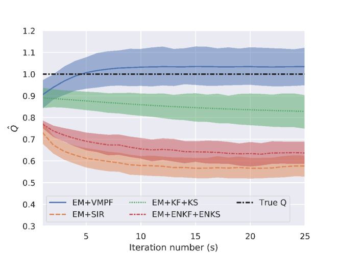
Figure 1: $\hat{\mathbf{Q}}$ as function of the iteration number using the EM + VMPF (blue), EM + SIR (orange) EM+KF+KS (green) and EM + EnKF + EnKS (red) algorithms, for the linear model 23 with true parameter value $\mathbf{Q}_{true}=\mathbf{I}_{1}$, $\mathbf{R}=\mathbf{I}_{1}$, $\nu=0.8$ and $K=100$. The 95$\%$ confidence interval were generated by running 50 independent repetitions of these estimation experiments and 25 EM iterations. For the EM + VMPF only $Np=20$ particles were used, whereas for the EM + SIR and the EM+EnKF+EnKS $N_{p}=1000$ particles and $N_{p}=50$ ensemble members, respectively, were used.

The mean and $95\%$ confidence intervals obtained by the 50 repetitions of the experiments with each algorithm are shown in Figure 1. As can be seen in Figure 1, although with a greater dispersion, the EM + VMPF algorithm starts to stabilize after as few as 4 iterations with its mean value very close to the true value $\mathbf{Q}_{true}=\mathbf{I}_{1}$. Despite having smaller variances and also stabilizing after a few iterations, the other algorithms provide estimates that are more biased. Moreover, the EM + EnKF + EnKS algorithm reaches an estimated value of 0.65 which represents a relatively large underestimation in coherence with the EM + KF + KS proposed in [26].

For this simple linear model and with $N_{p}$ = 1000 particles, the results obtained by using the SIR filter were similar to those obtained by the EM + EnKF + EnKS proposal, and not as good in terms of bias and RMSE as the ones obtained by using the VMPF with only $N_{p}=20$ particles. In the experiments that follow, we only use EM+VMPF for the particle filter implementation of the proposed algorithm. Experiments coupling the EM algorithm with the SIR filter for high-dimensional state and observational spaces, including the Lorenz-96 system, are not feasible due to the large number of particles required [21].

In order to analize the sensitivity of the algorithm to different observation error variances $\mathbf{R}$, we conducted some experiments similar to the ones described above, for different values of $\mathbf{R}\in\{0.1\mathbf{I}_{1},0.5\mathbf{I}_{1},\mathbf{I}_{1}\}$. The estimates of the model error covariance $\mathbf{Q}$ (mean value of 50 independent repetitions of the same experiment) and $95\%$ confidence intervals as a function of the iteration number of the EM + VMPF and EM + EnKF + EnKS algorithms are shown in fig. 2. Both algorithms stabilize in as few as 5 - 10 iterations, with the EM + VMPF less biased, independent of the value of $\mathbf{R}$. Even for a small observation error variance $\mathbf{R}$, the $95\%$ confidence interval obtained by the EM + EnKF + EnKS proposal does not reach the true value $\mathbf{Q}=\mathbf{I}_{1}$.

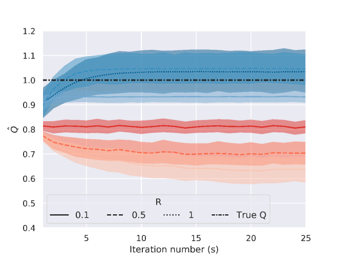
Figure 2: $\hat{\mathbf{Q}}$ as a function of the iteration number using the EM+VMPF algorithm (blue), and the EM+KF+KS algorithm (red) for the linear model 23 with true parameter values $\mathbf{Q}_{true}=\mathbf{I}_{1}$, $\nu=0.8$, different values of $\mathbf{R}$ and $K=100$. For the algorithm here proposed (EM + VMPF) only $Np=20$ particles were used, whereas for the EM+EnKF+EnKS $N_{e}=50$ ensemble members were used.

3.2 Lorenz-96 model

In this section we show results of twin experiments using the chaotic and nonlinear Lorenz-96 system as the dynamical model $\mathcal{M}$ in equation 1. The Lorenz-96 is one of the most used toy models in data assimilation within the geoscience community due to its ability to mimic certain properties of the atmospheric predictability at a low computational cost.

It is defined by the ordinary differential equations

$$\frac{\mathrm{d}X_{n}}{\mathrm{d}t}=-X_{n-2}X_{n-1}+X_{n-1}X_{n+1}-X_{n}+F,$$ (24)

where $X_{n}$ is the state variable of the model at variable (position) $n$, $n=1,\ldots,N_{x}$ and the domain is assumed periodic, that is, $X_{-1}\equiv X_{N-1}$, $X_{0}\equiv X_{N}$, $X_{N+1}\equiv X_{1}$. $F$ is the forcing constant and as usual, here it is set $F=8$ to represent chaotic dynamics.

We used a fourth-order Runga-Kutta scheme, with a model time step of $\delta_{t}=0.005$ to integrate the Lorenz-96 equations eq. 24. In these first set of experiments with the Lorenz-96 system, the number of variables is set to $N_{x}=8$, meaning that 64 parameters have to be estimated as the model error covariance $\mathbf{Q}$ is an $8\times 8$ matrix. The observation error covariance $\mathbf{R}$ was chosen as a diagonal matrix $\mathbf{R}=\sigma_{R}^{2}\mathrm{\bf I}$. We observed every grid point, in other words, the observation model $\mathcal{H}$ is assumed to be the identity transformation. The observations are taken every $\Delta_{t}=0.05$ which represents 10 model time steps in all the experiments performed.

For these twin experiments, we simulated $K=500$ noisy observations $\mathbf{y}_{1:K}$ using the Lorenz-96 model with known model error and observation error covariances $\mathbf{Q}_{true},\mathbf{R}$. Using the same model and these synthetic observations, the full model error covariance matrix $\mathbf{Q}$ was estimated.

The particle filter used in all the experiments performed was the VMPF with $N_{p}=20$ particles. The results are compared with the ones from the EM + EnKF+EnKS algorithm with also $N_{p}=20$ ensemble members.

To assess the proposed methodology to estimate the model error covariance matrix, experiments with two different structures, usually assumed in practice, were proposed for the true model error covariance matrix $\mathbf{Q}_{true}$: a) an isotropic non correlated covariance matrix, where $\mathbf{Q}_{true}=\sigma^{2}\mathrm{\bf I}$, with $\mathrm{\bf I}$ the identity matrix of order $N_{x}$ and b) an isotropic tridiagonal covariance matrix with diagonal values $\sigma_{d}^{2}$ and both sub-/super-diagonal values $\sigma_{sd}^{2}$. In the first case we assume that model errors for different model variables are uncorrelated and have the same variance $\sigma_{d}^{2}$, whereas for the second case we assume an a priori spatial covariance structure with correlations between the first neighbours.

Following a similar procedure as for the linear model case (section 3.1), $50$ independent realizations of this experiment were performed in order to show the estimator empirical distribution and to analyze its sensitivity to initial guesses $Q_{0}$ and random sampling of the observations. The non zero values of the initial guesses $Q_{0}$ (a $N_{x}\times N_{x}$ matrix with the same structure of $\mathbf{Q}_{true}$), $\sigma_{d}^{2}$ and $\sigma_{sd}$, were sampled from $\mathcal{U}[0.05,0.5]$ and $\mathcal{U}[0.01,0.15]$, respectively.

In fig. 3 we show the empirical distribution of the estimator of $\mathbf{Q}$ (top panel) for true parameter value $\mathbf{Q}_{true}=\sigma^{2}\mathrm{\bf I}$ with $\sigma^{2}=0.2$, $\mathbf{R}=0.5\mathrm{\bf I}$ and $K=500$ observations, the distribution of the mean of the absolute values of the off-diagonal elements of $\hat{\mathbf{Q}}_{(s)}$ (middle panel) and the Frobenius norm $\lVert\mathbf{Q}_{true}-\hat{\mathbf{Q}}_{(s)}\rVert_{F}$ (bottom panel), for the algorithm proposed in this work, EM+VMPF (blue) and the EM+EnKF + EnKS algorithm (red) proposed by [20], that requires an ensemble Kalman smoother.

For ease of visualization, and just for plotting purposes, in this case of an isotropic uncorrelated covariance assumption $\mathbf{Q}=\sigma^{2}\mathrm{\bf I}$, at the s-th iteration of the EM algorithm we kept $[\widehat{\sigma_{d}^{2}}]_{s}$ as the average of the diagonal values of $\widehat{\mathbf{Q}}_{(s)}$. As we repeated each experiment independently 50 times, we have a series of 50 values of $[\widehat{\sigma_{d}^{2}}]_{s}$ at the $s$ iteration of the EM-algorithm to construct a violin object that describes the empirical distribution of the corresponding estimator at each iteration.

With only $N_{p}=20$ particles both methods provide good estimates of $\mathbf{Q}$, stabilizing in about 10 iterations with its median value (white circle) around the true diagonal value (top panel). The EM+ VMPF (blue) algorithm produces estimates less biased than the EM + EnKF + EnKS (red) despite the fact that it does not require a particle smoother (and therefore uses less observational information in the state estimates). More over, the violin objects show that the empirical distribution for the EM + VMPF estimates is symmetric and highly concentrated around the true value, whereas the EM+EnKF+EnKS estimates empirical distributions have a greater dispersion, are not symmetric and have tails towards higher values of $\sigma_{d}^{2}$, meaning that in the 50 repetitions performed this method overestimates the value of $\sigma_{d}^{2}$. The middle panel of fig. 3 shows the distribution of the mean of the absolute values of the off-diagonal elements of $\hat{\mathbf{Q}}_{(s)}$. Both methods provide reasonable estimates of the off-diagonal elements (should be zero), with the EM+EnKF+EnKS better. The bottom panel of the same figure shows the empirical distribution of the Frobenius norm $\lVert\mathbf{Q}_{true}-\hat{\mathbf{Q}}_{(s)}\rVert_{F}$ for both methods. Again, the EM + EnKF + EnKS (red), despite having a greater dispersion has a slightly better performance.

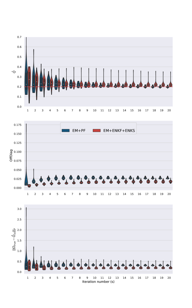
Figure 3: EM+ VMPF (blue) and EM + EnKF + EnKS (red) performances when estimating $\mathbf{Q}$ (top), mean of the absolute value of the off-diagonal elements of $\hat{\mathbf{Q}}_{(s)}$ and Frobenius norm $\lVert\mathbf{Q}_{true}-\hat{\mathbf{Q}}_{(s)}\rVert_{F}$ and loglikelihood function $l(\hat{\mathbf{Q}}_{(s)})$ for the Lorenz-96 model 24 with true model error covariance $\mathbf{Q}_{true}=\sigma^{2}\mathrm{I}$, with $\sigma^{2}=0.2$, and $K=500$. The violin plots were generated by running 50 independent repetitions of the algorithm with $Np=20$ particles and keeping the average of the diagonal values of $\hat{\mathbf{Q}}_{s}$

To analyze the sensitivity of the proposed algorithm to different values of the observation error covariance $\mathbf{R}$ a second set of experiments was performed. We assumed $\mathbf{R}=\sigma_{R}^{2}\mathbf{I}$ with $\sigma_{R}^{2}\in\{0.1,0.5,1.0,2.0\}$, and $\mathbf{Q}=0.2\mathbf{I}$. For each setting we performed 30 independent realizations of the same experiment. The mean and $95\%$ confidence intervals for $[\widehat{\sigma^{2}_{d}}]_{s}$ for each value of $\sigma_{R}^{2}$ are shown in fig. 4. The larger $\mathbf{R}$ values, the harder to estimate model error likely because of sampling noise. The results for $\sigma_{R}^{2}=1.0$ and 2.0 are noisier and demonstrate small biases, even after 25 iterations of the EM scheme. As clearly stated in [30] and references therein, the quality of reconstructed state vectors and estimation procedures when using variational or ensemble-based methods, largely depends on the relative amplitudes between observation and model errors. In [40] the authors also mention that a small increment in the magnitude of the observation error $\mathbf{R}$ highly affects the accuracy and behaviour of the method they propose to estimate the model error $\mathbf{Q}$ iteratively in the observation space using the implicit equally weighted particle filter (IEWPF) [39]. Their method provides reasonable estimates of the diagonal values of $\mathbf{Q}_{true}$ as long as the diagonal values of the observation error matrix $\mathbf{R}$ are relatively small (they assume a diagonal $\mathbf{R}$), with $\sigma_{R}^{2}=0.2$ the largest one. The larger $\sigma_{R}^{2}$, the less accurate the estimation procedure. As shown in fig. 4, the estimation with the EM+VMPF gives results with a good performance for observational variances ranging from 0.1 to 2.0. The estimation error increases with the increase of the observational variance, however, the estimation error is lower than 20% in all the cases shown.

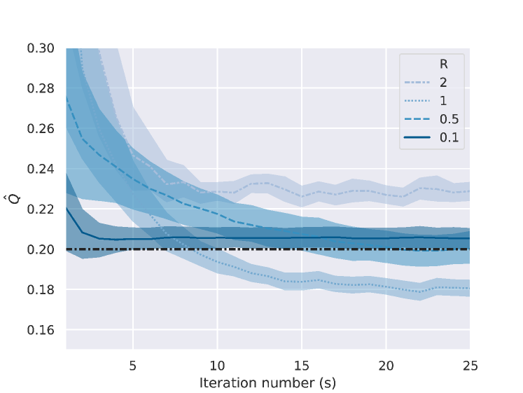
Figure 4: Sensitivity of EM+VMPF to different values of observation error $\mathbf{R}$ with true model error covariance $\mathbf{Q}_{true}=\sigma^{2}\mathrm{I}$, with $\sigma^{2}=0.2$, and $K=500$.

Experiments designed for the estimation of a tridiagonal isotropic model error covariance are shown in fig. 5. The diagonal value of $\mathbf{Q}_{true}$ was set to $\sigma_{d}^{2}=0.2$ and sub-/super-diagonal values were $\sigma_{sd}^{2}=0.05$, as defined in [40], $\mathbf{R}=0.5\mathrm{\bf I}$, $K=500$, $N_{p}=20$. For this isotropic tridiagonal model error covariance assumption, at the s-th iteration of the EM algorithm we computed $\widehat{\sigma^{2}_{d}}$ as the average of the diagonal values of $\hat{\mathbf{Q}}_{s}$, and $\widehat{\sigma^{2}_{sd}}$ as the average of the sub-/super-diagonal values of $\hat{\mathbf{Q}}_{s}$. The violin plots at the s-th iteration of the EM algorithm were generated with $\widehat{\sigma^{2}_{d}}$, $\widehat{\sigma^{2}_{sd}}$ obtained for each realization of the experiment.

As shown in fig. 5 both the EM+VMPF(blue) and EM+EnKF+EnKS (red) methods converges rapidly to the true value $\sigma_{d}^{2}$ (top panel). The empirical distribution of the EM+VMPF estimates shows a median value (white circle) closer to the true value of $\sigma_{d}^{2}$ but has a greater dispersion. However, as in the diagonal $\mathbf{Q}$ case, the EM+EnKF+EnKS proposal tends to overestimate $\sigma_{d}^{2}$. Both methods show a similar performance when estimating the sub-/super-diagonal elements of $\mathbf{Q}$, with the EM+VMPF more biased in terms of the median value. However, after 17 iterations the violin object obtained by the EM+VMPF proposal is completely contained within the violin object obtained by the EM+EnKF+EnKS algorithm. A different behaviour is observed for the empirical distribution of the Frobenius Norm. In this case, the EM+EnKF+EnKS always outperforms the EM+VMPF estimation procedure.

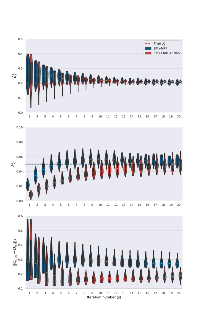
Figure 5: Estimation of $\mathbf{Q}$ as a function of the iteration for the EM+VMPF (blue) and EM+EnKF+EnKS (red) for the Lorenz-96 model with tridiagonal true model error covariance $\mathbf{Q}_{true}$, with $\sigma_{d}^{2}=0.2$, $\sigma_{sd}^{2}=0.05$ and $K=500$. The violin plots were generated by running 50 independent repetitions of these algorithms with $N_{p}=20$ particles. Upper panels show the average of the estimated diagonal values of $\hat{\mathbf{Q}}_{s}$ (top panel) and the average of the sub/super-diagonal values of $\hat{\mathbf{Q}}_{s}$ (middle panel). Frobenius norm $\lVert\mathbf{Q}_{true}-\hat{Q}_{(s)}\rVert_{F}$ (bottom panel) as function of the algorithm iteration.

In most of the experiments performed the proposed method converges to the true diagonal value of $\mathbf{Q}$ after a few iterations, tending to slightly overestimate the sub-/super-diagonal values of $\mathbf{Q}$.

A higher dimensional experiment was also performed for a chaotic Lorenz-96 model with 40 dimensions and $F=8$. In this case, the number of parameters to be estimated is $40\times 40=1600$. Estimations of model error covariances from 20 repetitions of this experiment for an isotropic uncorrelated model error covariance $\mathbf{Q}=0.2\ \mathbf{I}$, with $\mathbf{R}=0.5\ \mathbf{I}$ and K = 250 observations are shown in fig. 6. Despite the increase in the dimensionality, the method provides unbiased results when estimating the diagonal values of $\mathbf{Q}$ after a few iterations (top panel), however the estimation of the off diagonal values and Frobenius norm of $\mathbf{Q}$ is slightly affected by the increase in dimensionality if compared to the $8\times 8$ case (cf. fig. 3).

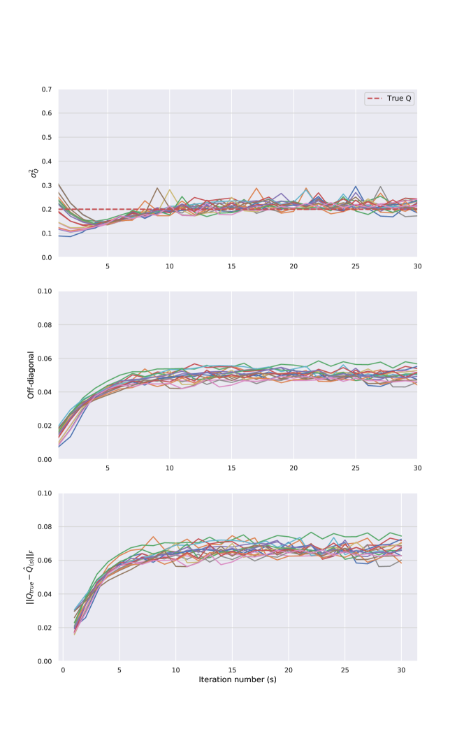
Figure 6: EM+VMPF results when estimating $\mathbf{Q}$ as a function of the iteration, for the 40th dimensional Lorenz-96 model with $\mathbf{Q}=0.2\ \mathbf{I}$, $\mathbf{R}=0.5\ \mathbf{I}$, $K=250$. Twenty independent repetitions of the same experiment were performed and each line shows the mean of the diagonal values of $\hat{\mathbf{Q}}_{s}$ (top panel), mean of the absolute value of the off-diagonal elements of $\hat{\mathbf{Q}}_{(s)}$ (middle panel) and Frobenius norm $\lVert\mathbf{Q}_{true}-\hat{\mathbf{Q}}_{(s)}\rVert_{F}$ (bottom panel) for each of these repetitions.

4 Conclusions

In this work a novel method to estimate the model error uncertainty in dynamical systems is introduced and evaluated. It assumes that both the model and observation errors are additive and Gaussian with zero mean and covariance matrices $\mathbf{Q}$ and $\mathbf{R}$, respectively. The methodology here presented is based on the maximization of a likelihood criterium using the principles of the EM algorithm and a particle filter. We aim at maximizing the complete likelihood of the observations by marginalizing this likelihood function. The resulting likelihood is expressed sequentially. By taking this approach, in the E-Step of the EM algorithm we only have to compute filtering densities avoiding the need to compute smoothing densities, which are known to be one of the main drawbacks when using particle filters in data assimilation. The trade-off of avoiding the need of a particle smoother in the E-Step of the EM algorithm is the need to solve an implicit equation for $\mathbf{Q}$ in the M-Step of the EM algorithm. This problem was tackled by means of a fixed point algorithm, and despite the fact that an analytical proof of its convergence is not straightforward to obtain due to the nonlinearity of the model dynamics, empirical results show that it converges to a solution of this implicit equation.

The EM algorithm coupled with the VMPF presents, in general, an overall excellent performance. It gives very promising results in the experiments performed with a simple linear first order autoregressive system and a chaotic Lorenz-96 system with 8 and 40 variables. In the first case, results were compared with those obtained by different methods already proposed in the literature, showing a good performance in terms of bias and RMSE, and being more robust to different values of the observation error $\mathbf{R}$. The new method is suitable for non-Gaussian posterior densities from nonlinear dynamical and observational models, unlike the Kalman Filter/Smoother and its ensemble variants.

In the case of the Lorenz-96 system, its performance was tested for different scenarios showing good convergence properties. It is stable even for $\mathbf{R}=10\mathbf{Q}$, although a small bias appears in the estimate. The new method outperforms the traditional EM algorithm with the EnKS [12] for a diagonal $\mathbf{Q}$ and for the diagonal of a tri-diagonal $\mathbf{Q}$. However, off-diagonal elements estimates were always noisier than those using an EnKS. It also works in high-dimensional estimation problems of dimensions over 1000 and state space of 40.

Model error covariances are essential in particle flow filters. The conducted experiments show that these particle flow filters, in particular VMPF, can work with an adaptative model error without apriori information on this covariance whereas in previous studies a fixed known model error covariance was used [21]. Model error covariances impact on the prior density and also on the kernel covariance in the VMPF. The overall excellent performance of the estimates may also trace back to the strong sensitivity of VMPF performance to model error covariance. In this sense, there is a positive feedback between the model error covariance estimates of the EM algorithm and the state estimates of the filter.

The computational cost of the algorithm here proposed is directly related to the number of iterations needed for convergence. All the experiments performed achieved convergence to a narrow neighbourhood of the true value of $\mathbf{Q}$ in as few as 10 to 15 iterations of the EM algorithm. Each EM iteration requires the computation of K filtering densities computed by using a particle filter with $N_{p}$ particles, whereas the M-Step requires to solve a fixed point algorithm. In our experiments we set the number of iterations for this fixed point algorithm to 6, based on empirical evidence. In turn, each of these fixed point iterations also require to compute K filtering densities computed by using a particle filter with $N_{p}$ particles.

5 Appendix A: Derivation of $\mathcal{G}(\theta^{\prime},\theta)$

As explained in section 2.3, the likelihood of the observations can be decomposed as $p(\mathbf{y}_{1:K};\theta)=\prod^{K}_{k=1}p(\mathbf{y}_{k}|\mathbf{y}_{k-1};\theta)$, with the convention $\mathbf{y}_{1:0}=\{\emptyset\}$. Marginalizing this last expression we obtain

$$p(\mathbf{y}_{1:K};\theta) =\prod^{K}_{k=1}p(\mathbf{y}_{k}|\mathbf{y}_{k-1};\theta)$$

$$=\prod^{K}_{k=1}\int p(\mathbf{y}_{k}|\mathbf{x}_{k};\theta)p(\mathbf{x}_{k}|\mathbf{y}_{1:k-1};\theta)\mathrm{d}\mathbf{x}_{k}$$ (25)

and taking logarithm we can rewrite this last expression as

$$l(\theta)=\log p(\mathbf{y}_{1:K};\theta)=\log\prod^{K}_{k=1}\int q_{\theta^{\prime}}(\mathbf{\mathbf{missing}}x_{k})\frac{p(\mathbf{y}_{k}|\mathbf{x}_{k};\theta)p(\mathbf{x}_{k}|\mathbf{y}_{1:k-1};\theta)}{q_{\theta^{\prime}}(\mathbf{\mathbf{missing}}x_{k})}\mathrm{d}\mathbf{x}_{k}$$

where $q_{\theta^{\prime}}(\mathbf{x}_{k})$ is a probability density function whose support includes the support of the likelihood of the observations. In principle, $\theta^{\prime}$ is not necessarily equal to $\theta$ . Using Jensen’s inequality,

$$l(\theta)\geq\sum_{k=1}^{K}\int q_{\theta^{\prime}}(\mathbf{x}_{k})\log\left(\frac{p(\mathbf{y}_{k}|\mathbf{x}_{k};\theta)p(\mathbf{x}_{k}|\mathbf{y}_{1:k-1};\theta)}{q_{\theta^{\prime}}(\mathbf{x}_{k})}\right)\mathrm{d}\mathbf{x}_{k}$$ (26)

Let $\mathcal{G}(q,\theta)$ be an intermediate function defined as

$$\mathcal{G}(q,\theta)=\sum_{k=1}^{K}\int q(\mathbf{x}_{k})\log\left(\frac{p(\mathbf{y}_{k}|\mathbf{x}_{k};\theta)p(\mathbf{x}_{k}|\mathbf{y}_{1:k-1};\theta)}{q(\mathbf{x}_{k})}\right)\mathrm{d}\mathbf{x}_{k}$$ (27)

Using Bayes rule, the recursive posterior density at time $k$ is

$$p(\mathbf{x}_{k}|\mathbf{y}_{1:k};\theta)=\frac{p(\mathbf{y}_{k}|\mathbf{x}_{k};\theta)p(\mathbf{x}_{k}|\mathbf{y}_{1:k-1};\theta)}{p(\mathbf{y}_{k}|\mathbf{y}_{1:k-1};\theta)}$$ (28)

If we choose $q(\mathbf{x}_{k})=p(\mathbf{x}_{k}|\mathbf{y}_{1:k};\theta)$, and so replacing eq. 28 in eq. 27,it can be shown that $\mathcal{G}(q,\theta)=l(\theta)$. That means that for fixed $\theta=\theta^{\prime}$, the function $q$ that maximizes the intermediate function, $\mathcal{G}$, is the recursive posterior density $p(\mathbf{x}_{k}|\mathbf{y}_{1:k};\theta)$. This density can be inferred by a filter method and this corresponds to the Expectation Step.

On the other hand, maximizing $\mathcal{G}(q,\theta)$, with respect to $\theta$ gives a lower bound of $l(\theta)$.

The maximization step consists in maximizing $\mathcal{G}(q^{\prime},\theta)$ as a function of $\theta$, where $q^{\prime}$ is the density obtained in the Expectation step. If we now write $q_{\theta^{\prime}}(\mathbf{x}_{k})=p(\mathbf{x}_{k}|\mathbf{y}_{1:k};\theta^{\prime})$, and make an abuse of notation in the expression $\mathcal{G}(q_{\theta^{\prime}},\theta)$ by replacing $q_{\theta^{\prime}}$ by the parameter that identifies it, then

$$\mathcal{G}(\theta^{\prime},\theta) =\sum_{k=1}^{K}\int p(\mathbf{x}_{k}|\mathbf{y}_{1:k};\theta^{\prime})\log\left(\frac{p(\mathbf{y}_{k}|\mathbf{x}_{k};\theta)p(\mathbf{x}_{k}|\mathbf{y}_{1:k-1};\theta)}{p(\mathbf{x}_{k}|\mathbf{y}_{1:k};\theta^{\prime})}\right)\mathrm{d}\mathbf{x}_{k}$$ (29)

$$=\sum_{k=1}^{K}\int p(\mathbf{x}_{k}|\mathbf{y}_{1:k};\theta^{\prime})\log\left(p(\mathbf{y}_{k}|\mathbf{x}_{k};\theta)p(\mathbf{x}_{k}|\mathbf{y}_{1:k-1};\theta)\right)\mathrm{d}\mathbf{x}_{k}$$ (30)

$$-\sum_{k=1}^{K}\int p(\mathbf{x}_{k}|\mathbf{y}_{1:k};\theta^{\prime})\log\left(p(\mathbf{x}_{k}|\mathbf{y}_{1:k};\theta^{\prime})\right)\mathrm{d}\mathbf{x}_{k}$$ (31)

6 Appendix B: Equation for $\mathbf{Q}$

We want to find the root of $\frac{\partial}{\partial\mathbf{Q}}\mathcal{G}(\mathbf{Q}_{s-1},\mathbf{Q})=0$, where $\mathcal{G}(\mathbf{Q}_{s-1},\mathbf{Q})$

$$\mathcal{G}(\mathbf{Q}_{s-1},\mathbf{Q})\doteq\sum_{k=1}^{K}\sum_{j=1}^{N_{p}}w_{k,\mathbf{Q}_{s-1}}^{(j)}\log\left(\sum_{i=1}^{N_{p}}w_{k-1,\mathbf{Q}}^{(i)}\ \ \mbox{\boldmath$\phi$}\left(x_{k}^{(j)},\mathcal{M}(\mathbf{x}_{k-1}^{(i)}),\mathbf{Q}\right)\right)$$

and $\mbox{\boldmath$\phi$}\left(\mathbf{x}_{k},\mbox{\boldmath$\mu$},\mbox{\boldmath$\Sigma$}\right)=\frac{1}{(2\pi)^{N_{x}/2}|\mbox{\boldmath$\Sigma$}|^{1/2}}\exp\left\{-\frac{1}{2}(\mathbf{x}_{k}-\mbox{\boldmath$\mu$})^{T}\mbox{\boldmath$\Sigma$}^{-1}(\mathbf{x}_{k}-\mbox{\boldmath$\mu$})\right\}$

Denoting $\mbox{\boldmath$\beta$}_{k}^{(i,j)}=\mathbf{x}_{k}^{(j)}-\mathcal{M}(\mathbf{x}_{k-1}^{(i)})$ we have

$$\frac{\partial}{\partial\mathbf{Q}}\mathcal{G}(\mathbf{Q}_{s-1},\mathbf{Q}) =$$

$$= \sum_{k=1}^{K}\sum_{j=1}^{N_{p}}w_{k,\mathbf{Q}_{s-1}}^{(j)}\frac{\partial}{\partial\mathbf{Q}}\log\left[\sum_{i=1}^{N_{p}}\frac{w_{k-1}^{(i)}}{(2\pi)^{N_{x}/2}|\mathbf{Q}|^{1/2}}\times\right.$$

$$\left.\exp\left\{-\frac{1}{2}(\mbox{\boldmath$\beta$}_{k}^{(i,j)^{T}}\mathbf{Q}^{-1}\mbox{\boldmath$\beta$}_{k}^{(i,j)})\right\}\right]$$

$$= \sum_{k=1}^{K}\sum_{j=1}^{N_{p}}w_{k,\mathbf{Q}_{s-1}}^{(j)}\frac{\partial}{\partial\mathbf{Q}}\left[-\frac{N_{x}}{2}\log(2\pi)-\frac{1}{2}\log|\mathbf{Q}|+\right.$$

$$\left.+\log\left(\sum_{i=1}^{N_{p}}w_{k-1}^{(i)}\exp\left\{-\frac{1}{2}(\mbox{\boldmath$\beta$}_{k}^{(i,j)^{T}}\mathbf{Q}^{-1}\mbox{\boldmath$\beta$}_{k}^{(i,j)})\right\}\right)\right]$$

$$=-\frac{K}{2}\mathbf{Q}^{-1}+\frac{1}{2}\mathbf{Q}^{-1}\left[\sum_{k=1}^{K}\sum_{j=1}^{N_{p}}w_{k,\mathbf{Q}_{s-1}}^{(j)}\ \frac{1}{S_{i}}\sum_{i=1}^{N_{p}}w_{k-1}^{(i)}\times\right.$$

$$\left.\times\exp\{-\frac{1}{2}(\mbox{\boldmath$\beta$}_{k}^{(i,j)^{T}}\mathbf{Q}^{-1}\mbox{\boldmath$\beta$}_{k}^{(i,j)})\}\mbox{\boldmath$\beta$}_{k}^{(i,j)}\mbox{\boldmath$\beta$}_{k}^{(i,j)^{T}}\right]\mathbf{Q}^{-1}$$

where $S_{i}=\sum_{i=1}^{N_{p}}w_{k-1}^{(i)}\exp\{-\frac{1}{2}(\mbox{\boldmath$\beta$}_{k}^{(i,j)^{T}}\mathbf{Q}^{-1}\mbox{\boldmath$\beta$}_{k}^{(i,j)})\}$

Thus, $\mathbf{Q}$ that satisfies $\frac{\partial}{\partial\mathbf{Q}}\mathcal{G}(\mathbf{Q}_{s-1},\mathbf{Q})=0$ is given by

$$\mathbf{Q} =\frac{1}{K}\sum_{k=1}^{K}\left[\sum_{j=1}^{Np}w_{k,\mathbf{Q}_{s-1}}^{(j)}\left(\frac{1}{S_{i}}\sum_{i=1}^{Np}w_{k-1,Q}^{(i)}\ \mbox{\boldmath$\psi$}_{k}^{j,i}\mathbf{B}_{k}^{j,i}\right)\right]$$ (32)

where

$\mbox{\boldmath$\psi$}_{k}^{j,i}=\exp\{-\frac{1}{2}(\mbox{\boldmath$\beta$}_{k}^{(i,j)^{T}}\mathbf{Q}^{-1}\mbox{\boldmath$\beta$}_{k}^{(i,j)})\}$

$\mathbf{B}_{k}^{j,i}=\mbox{\boldmath$\beta$}_{k}^{(i,j)}\mbox{\boldmath$\beta$}_{k}^{(i,j)^{T}}$

Acknowledgements: This work was funded by European Research Council (ERC) CUNDA project 694509 under the European Union Horizon 2020 research and innovation programme.

References

- [1] M. S. Arulampalam, S. Maskell, N. Gordon, and T. Clapp, A tutorial on particle filters for online nonlinear/non-gaussian bayesian tracking, IEEE Transactions on signal processing, 50 (2002), pp. 174–188.
- [2] M. Briers, A. Doucet, and S. Maskell, Smoothing algorithms for state–space models, Annals of the Institute of Statistical Mathematics, 62 (2010), p. 61.
- [3] P. Bunch and S. Godsill, Approximations of the optimal importance density using gaussian particle flow importance sampling, Journal of the American Statistical Association, 111 (2016), pp. 748–762.
- [4] O. Cappé, E. Moulines, and T. Ryden, Inference in Hidden Markov Models, Springer Science & Business Media, 2006.
- [5] A. Carrassi, M. Bocquet, A. Hannart, and M. Ghil, Estimating model evidence using data assimilation, Quarterly Journal of the Royal Meteorological Society, 143 (2017), pp. 866–880.
- [6] R. Daley, Atmospheric data analysis, no. 2, Cambridge university press, 1993.
- [7] F. Daum, J. Huang, and A. Noushin, Exact particle flow for nonlinear filters, in Signal Processing, Sensor Fusion, and Target Recognition XIX, vol. 7697, International society for optics and photonics, 2010, p. 769704.
- [8] A. P. Dempster, N. M. Laird, and D. B. Rubin, Maximum likelihood from incomplete data via the em algorithm, Journal of the Royal Statistical Society: Series B (Methodological), 39 (1977), pp. 1–22.
- [9] R. Douc, E. Moulines, and D. Stoffer, Nonlinear time series: Theory, methods and applications with R examples, Chapman and Hall/CRC, 2014.
- [10] A. Doucet and A. M. Johansen, A tutorial on particle filtering and smoothing: Fifteen years later,2009.
- [11] M. Dowd, E. Jones, and J. Parslow, A statistical overview and perspectives on data assimilation for marine biogeochemical models, Environmetrics, 25 (2014), pp. 203–213.
- [12] D. Dreano, P. Tandeo, M. Pulido, B. Ait-El-Fquih, T. Chonavel, and I. Hoteit, Estimating model-error covariances in nonlinear state-space models using kalman smoothing and the expectation–maximization algorithm, Quarterly Journal of the Royal Meteorological Society, 143 (2017), pp. 1877–1885.
- [13] N. J. Gordon, D. J. Salmond, and A. F. Smith, Novel approach to nonlinear/non-gaussian bayesian state estimation, in IEE proceedings F (radar and signal processing), vol. 140, IET, 1993, pp. 107–113.
- [14] N. Gupta and R. Mehra, Computational aspects of maximum likelihood estimation and reduction in sensitivity function calculations, IEEE Transactions on Automatic Control, 19 (1974), pp. 774–783.
- [15] N. Kantas, A. Doucet, S. S. Singh, J. Maciejowski, N. Chopin, et al., On particle methods for parameter estimation in state-space models, Statistical science, 30 (2015), pp. 328–351.
- [16] K. Law, A. Stuart, and K. Zygalakis, Data assimilation, Springer, 2015.
- [17] E. N. Lorenz, Predictability: A problem partly solved, in Proc. Seminar on predictability, vol. 1, 1996.
- [18] P. Matisko and V. Havlena, Noise covariance estimation for kalman filter tuning using bayesian approach and monte carlo., Int J Adapt Control Signal Process, 27 (2013), pp. 957–973.
- [19] J. Olsson, O. Cappé, R. Douc, E. Moulines, et al., Sequential monte carlo smoothing with application to parameter estimation in nonlinear state space models, Bernoulli, 14 (2008), pp. 155–179.
- [20] M. Pulido, P. Tandeo, M. Bocquet, A. Carrassi, and M. Lucini, Stochastic parameterization identification using ensemble kalman filtering combined with maximum likelihood methods, Tellus A: Dynamic Meteorology and Oceanography, 70 (2018), pp. 1–17.
- [21] M. Pulido and P. J. vanLeeuwen, Kernel embedding of maps for sequential bayesian inference: The variational mapping particle filter, Journal of Computational Physics, 396 (2019), pp. 400–415.
- [22] M. Pulido, P. J. vanLeeuwen, and D. Posselt, Kernel embedded nonlinear observational mappings in the variational mapping particle filter., Lecture Notes on Computational Sciences, ICCS-2019, (2019), pp. 141–155.
- [23] C. Robert and G. Casella, Monte Carlo statistical methods, Springer Science & Business Media, 2013.
- [24] N. Santitissadeekorn and C. Jones, Two-stage filtering for joint state-parameter estimation., Monthly Weather Review, 143 (2015), pp. 2028–2042.
- [25] G. Scheffler, J. Ruiz, and M. Pulido, Inference of stochastic parameterizations for model error treatment using nested ensemble kalman filters, Q. J. Roy. Met. Soc., 145 (2019), pp. 2028–2045.
- [26] R. Shumway and D. Stoffer, Time Series Analysis and Its Applications: With R Examples, Springer, 2010.
- [27] R. H. Shumway and D. S. Stoffer, An approach to time series smoothing and forecasting using the em algorithm, Journal of Time Series Analysis, 3 (1982), pp. 253–264.
- [28] L. M. Stewart, S. L. Dance, and N. K. Nichols, Data assimilation with correlated observation errors: experiments with a 1-d shallow water model, Tellus A: Dynamic Meteorology and Oceanography, 65 (2013), p. 19546.
- [29] J. Stroud and T. Bengtsson, Sequential state and variance estimation within the ensemble kalman filter, Mon Weather Rev., 135 (2007), pp. 3194–3208.
- [30] P. Tandeo, P. Ailliot, M. Bocquet, A. Carrassi, T. Miyoshi, M. Pulido, and Y. Zhen, Joint estimation of model and observation error covariance matrices in data assimilation: a review, arXiv preprint arXiv:1807.11221, (2018).
- [31] G. Ueno, T. Higuchi, T. Kagimoto, and N. Hirose, Maximum likelihood estimation of error covariances in ensemble-based filters and its application to a coupled atmosphere–ocean model, Quarterly Journal of the Royal Meteorological Society, 136 (2010), pp. 1316–1343.
- [32] G. Ueno and N. Nakamura, Iterative algorithm for maximum-likelihood estimation of the observation-error covariance matrix for ensemble-based filters, Quarterly Journal of the Royal Meteorological Society, 140 (2014), pp. 295–315.
- [33] G. Ueno and N. Nakamura, Bayesian estimation of the observation-error covariance matrix in ensemble-based filters, Quarterly Journal of the Royal Meteorological Society, 142 (2016), pp. 2055–2080.
- [34] P. J. Van Leeuwen, Particle filtering in geophysical systems, Monthly Weather Review, 137 (2009), pp. 4089–4114.
- [35] J. Waller, S. Dance, and N. Nichols, On diagnosing observation-error statistics with local ensemble data assimilation, Quarterly Journal of the Royal Meteorological Society, 143 (2017), pp. 2677–2686.
- [36] G. C. Wei and M. A. Tanner, A monte carlo implementation of the em algorithm and the poor man’s data augmentation algorithms, Journal of the American statistical Association, 85 (1990), pp. 699–704.
- [37] C. K. Wikle and L. M. Berliner, A bayesian tutorial for data assimilation, Physica D: Nonlinear Phenomena, 230 (2007), pp. 1–16.
- [38] C. J. Wu et al., On the convergence properties of the em algorithm, The Annals of statistics, 11 (1983), pp. 95–103.
- [39] M. Zhu, P. J. Van Leeuwen, and J. Amezcua, Implicit equal-weights particle filter, Quarterly Journal of the Royal Meteorological Society, 142 (2016), pp. 1904–1919.
- [40] M. Zhu, P. J. van Leeuwen, and W. Zhang, Estimating model error covariances using particle filters, Quarterly Journal of the Royal Meteorological Society, 144 (2018), pp. 1310–1320.