The effect of particle gas composition and boundary conditions on triboplasma generation: a computational study using the particle-in-cell method

Abstract

Two dimensional particle in cell simulations of free charge creation by collisional ionization of C12 and C60 molecules immersed in plasma for the parameters of relevance to plasma gasification are presented. Our main findings are that (i) in uniform plasmas with smooth walls two optimal values which emerge for free electron production by collisional ionization (i.e. a most efficient discharge condition creation) are $C60:C12$ fractions of $10:90$ and $80:20$, (ii) in plasmas with rough walls, modelled by comb-like electric field at the boundary, the case of tangential electric field creates significant charge localization in C12+ and C60+ species, again creating most favorable discharge condition for tribo-electrically generated plasma. The numerical simulation results are discussed with reference to recent triboelectric plasma experiments and are corroborated by suitable analytical models.

I Introduction

With the depletion of fossil resources and the mounting quantity of waste, energy generation and waste disposal have become very important problems of modern society. Waste-to-energy (WTE) approaches which aim to generate energy as heat or power from waste can provide a balanced solution to both these problems. One of the most promising WTE technologies is associated with the recuperation of energy via transforming non-recyclable materials through a combination of different high temperature-involving procedures such as waste gasification and pyrolysis. The advantages of the above thermal techniques over the conventional WTE techniques such as incineration and combustion include higher recycling rates, lower toxic gas emissions, higher energy efficiencies, lower costs, smaller carbon footprints and reduced environmental impact ref (2004). Importantly, gasification converts solid waste into a highly fungible synthetic gas (or syngas) very rich in hydrogen and carbon monoxide, that can be converted into clean electricity or other high value fuels/chemicals, including methanol, SNG (synthetic natural gas) or pure hydrogen Siedlecki and de Jong (2011); Meng et al. (2011); Na et al. (2003).

The use of plasma power has been popular within thermal waste treatments for its ability to completely decompose the input waste material into a tar-free synthetic gas and an inert, environmentally stable, vitreous material (slag) and preparing the syngas for efficient electricity production or catalytic transformation Helsen and Bosmans (2010). Because of the potential advantages, plasma technologies have been developed for the destruction and removal of various hazardous wastes, such as polychlorinated biphenyls (PCBs) Kim et al. (2003), medical waste Nema and Ganeshprasad (2002a), metallurgical wastes, incineration fly ash Nema and Ganeshprasad (2002b), and low-level radioactive wastes.

In addition to the waste gasification, plasma assisted combustion is a very active topic of research on its own right, which covers the topic ignition enhancement, ultra-lean combustion, cool flames, flameless combustion, and controllability of plasma discharge Ju and Sun (2015).

Currently, in many engineering applications plasma have been generated by constant current or electromagnetic field for which an external supply of electric energy is needed. For example, in the existing plasma gasification technologies, only additions of combustion heat supplied by the waste feedstock or a fuel additive make the process suited to large waste streams Ducharme and Themelis (2010). The main cost of the current plasma power technologies is associated with the energy required to artificially create significant electromagnetic or electrostatic fields to trigger and sustain gas discharges. For example, for dry air, few MVm^-1 is required to trigger a corona discharge Loeb (1965). This is of the same order of magnitude as the maximum power generated by the conventional high-energy particle accelerators. Such limit is due to the radio frequency (RF) breakdown phenomenon: when such large electric field is used in the accelerator cavities, it causes accelerator to be effectively short-circuited in accordance with the so-called Kilpatrick limit Kilpatrick (1957). Notably, this limit is overcome in novel accelerators which are based on plasmas, the so-called plasma wake field acceleration, and which can sustain electric fields up to tens of GVm^-1, without electric short-circuiting Tsiklauri (2019, 2016).

To trigger the discharge, hence creating plasma, electrodes powered by direct current are typically used Materazzi et al. (2016) . Altogether, the high cost of conventional plasma generators and short working life-time of electrodes (circa 500 hours) encourages researchers to consider other sources of plasma generation which do not need either the external electro-magnetic field or the electrodes.

Triboelectricity, or electricity generation by mechanical friction, can provide such an alternative source of plasma generation. An example of triboelectric charging in nature is the ash produced from the volcanic eruption that collides with one another producing significant charging which is discharged through lightning strikes.

Triboelectric plasma generation to ultimately replace the expensive direct current operated plasma torches can greatly improve efficiency of modern waste-to-energy gasification schemes while maintaining a very low emission signature.

In a recent laboratory experiment Gharib et al. (2017) the generation of plasma through a triboelectric effect was reported by impinging a high-speed (150-200 m/s) microjet of deionised water on a dialectric surface. A naturally formed, stable, unconstrained and topologically coherent triboplasma region in the form of a coherent toroidal structure was obtained in atmospheric pressure conditions without any external electromagnetic action.

An example of triboelectric plasma generation technology is the gasifier apparatus pioneered by LCC Engineering. In this case, a triboplasma region is generated by collision of ash particles (mostly carbon-based) in a swirling hydrodynamic flow generated by two tangential flow streams at a moderate flow speed (50 m/s) that grazes a serrated surface of an insulated steel wall. A schematic of the LCC Engineering apparatus is shown in Fig.1.

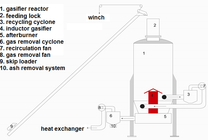
Figure 1: Schematic of the triboplasma gasifier apparatus of Engineering Company Eco-Ardens.

Here the organic fuel (e.g. chicken farm waste) is supplied from the top of the reactor and dropped through the triboplasma zone in the centre (above the ’inductor gasifier’ on the schematic). Because of a very high temperature in the centre of the reactor chamber, the waste is very efficiently decomposed into useful syngas, ash and a chemically inert slag, with virtually zero emission of toxic gases. Under the effect of particle-wall and particle-particle collisions, spark discharges are triggered, whose intensity grows as the tribo-electric self-charging of gas particles increases until a self-sustained localised tribo-plasma region emerges in the reaction zone (Fig.2).

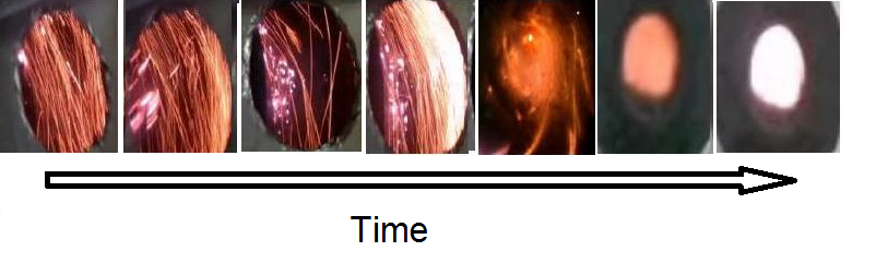
Figure 2: A rendered series of snapshots through the viewing window of the tribo-plasma gasifier apparatus of Engineering Company Eco-Ardens. From left to right: an initial to a developed stage of the tribo-plasma generation. The window location is in the centre of the reactor above the ’inductor’.

Among several fundamental issues, which remain to be understood before the tribolectric plasma generation can be used in real-life gasification applications, the following two questions stand out:

• According to the preliminary experimental results of Engineering Company Eco-Ardens, gas samples which correspond to successful triboelectric plasma generation are also rich in fullerenes (C60). Fullerenes are nano-size, football-like, carbon molecules which have a low ionization potential in comparison with hydrocarbons and a large surface-to-volume ratio in comparison with macroscopic soot particles. They are known to be readily generated in carbon plasmas through a non-equilibrium growth process that involves dehydrogenation of hydrocarbons, nucleation of large carbon cages and carbon cage evaporation to produce the small highly symmetry fullerenes such as C60 or C70. The particular question addressed in this work - what is effect of fullerenes on triboelectric charging of a gas mixture that includes both C60 and the standard carbon (C12) molecules?

• The triboelectric charge generation is dependent not only on the particulates present but also on the gas particle collisions with the uneven surfaces of the insulated conducting walls. How do the particle interactions with the wall can lead to an intensification of the triboelectric plasma effect?

To address the above questions, we use the state-of-the art EPOCH, fully kinetic particle-in-cell (PIC) code for solving kinetic plasma equations with a self-consistent field formulation Arber et al. (2015). To keep the particle in plasma simulations computationally feasible, a two-dimensional model of initially neutral carbon particles, C12 and C60, which are immersed into a fully ionized hydrogen plasma, is considered. In this model, the computational domain is covered by a Eulerian computational grid where the electromagnetic field equations are solved with capturing the characteristic Debye length. Clusters of neutral and charged carbon species as well as the free electrons are represented by Lagrangian particles which collide with including all relevant collision effects. The collision results in a new charge generation which is analysed for different concentrations of C60 and different boundary conditions to simulate the effect in the LCC Engineering experiment.

By analyzing the collisional ionization process it is shown that the rate of the new charge production from collisional ionization between carbon particles becomes greatly amplified once the concentration of fullerenes added to the gas exceeds a certain threshold value (circa 10% by number per volume fraction). Additional simulations reveal that the introduction of a non-periodic boundary condition imitating a serrated conducting wall of the experiment leads to a non-uniform concentration of the carbon particles and enhances the collision process thereby further enabling the increase of electric charge generation in the volume.

II The model and results

II.1 Methods

Two key phenomena which affect the triboelectric plasma generation are particle collisions and ionization. Hence, below we briefly discuss how these effects are implemented in the Particle-In-Cell EPOCH model Arber et al. (2015). It can be noted that many PIC models neglect particle collisions over very short (less than grid scale) ranges. At temperatures ($\gtrsim$ 1 keV) and number densities ($\lesssim 10^{27}$m^-3) collisional effects in plasmas are generally considered negligible. This implies that the mean time between collisions is comparable to the time scales of interest, and the collisionless approximation used in PIC codes is valid. However, at lower temperatures and/or higher densities the effect of sub-grid scale interactions on the evolution of the system can become non-negligible.

The maximum temperature in plasma gasifiers can reach a few $10^{4}$ K (recall that 1 keV corresponds to $1.16\times 10^{7}$ K), i.e. of the order if 1 eV. Typical plasma gasifier density is not readily available, but according to NRL Plasma Formulary, high pressure arcs have number densities of $10^{22-24}$ m^-3. Hence, collisional effects for gasifier setting are important.

A binary collision algorithm, based on the approach of Sentoku and Kemp has been implemented in EPOCH. To simplify momentum conservation treatment, collisions are calculated in the centre-of-momentum reference frame of the two particles. Lorentz transformations are included in order to evaluate the particles’ momenta in the centre-of-momentum frame. This ensures that in EPOCH collision algorithm is fully relativistic. EPOCH includes a number of different ionization models. These account for the different modes by which electrons ionize in both the external field (e.g. of an intense laser) and through collisions. To switch on collisions and collisional ionization in EPOCH an input file is used (input.deck). Four species included in the simulation are electrons, protons, C12, and C60. C12 has two possible ionization energies, 11.26 eV and 24.38 eV. The particles are immersed into a fully ionized plasma at temperature T=$10^{5}$ K where the number density of electrons and protons is set to $n=10^{15}$ m^-3.

End simulation time in most runs where there is no electric field forcing applied at the boundary is set to $t_{end}=11000/\omega_{pe}$ (Fig. 3-7). In the case of driving electric field at the boundary (Fig. 9-11) to simulate the wall effect, the end time is longer, $t_{end}=20000/\omega_{pe}$ to make sure that the solution reaches a more-or-less statistically converged state at least for some of the considered forcing regimes.

First, the simulations are performed in a homogenous domain, without accounting for the effect of the uneven wall of the gasifier. The boundary conditions are periodic in the x-direction for both the Electro-Magnetic (EM) fields and the particles and (ii) conducting in the y-direction for the fields and reflecting for the particles. Different grid cell and particle density resolutions, as well as the domain sizes, are considered (Fig. 3). Simulation results shown in figs. 4-8 correspond to the grid resolution of $288\times 72$ with each cell being 2 Debye length, i.e. $\Delta=2\lambda_{D}$, with $\lambda_{D}=V_{th,e}/\omega_{pe}$. The concentration of C12 and C60 species is varied so that total density stays the same. For example, $C60:C12$ fraction of $99:1$ means that $n_{C60}=n\times 99/100$ while $n_{C12}=n\times 1/100$, with $n$ being $n=10^{15}$ m^-3 number density for both electrons and protons. Similarly, $C60:C12$ fraction of $25:75$ means that $n_{C60}=n\times 25/100$ while $n_{C12}=n\times 75/100$, and so on.

Secondly, the case of driving the electric field on the bottom wall boundary is considered. Periodic boundary conditions in the x- and y- directions for both the EM fields and the particles are imposed. The latter choice is to make sure that driving of the periodic boundary condition to a prescribed forcing field is fully consistent with the governing discretisation of Maxwell’s equations. Results of these simulations are shown in figs. 9-11 which have grid resolution of $144\times 36$, with each cell being $\Delta=4\lambda_{D}$. The increased cell size is in order to have the same size of the computational domain in most simulation cases, with or without the electric field forcing.

II.2 Homogeneous particle interaction problem

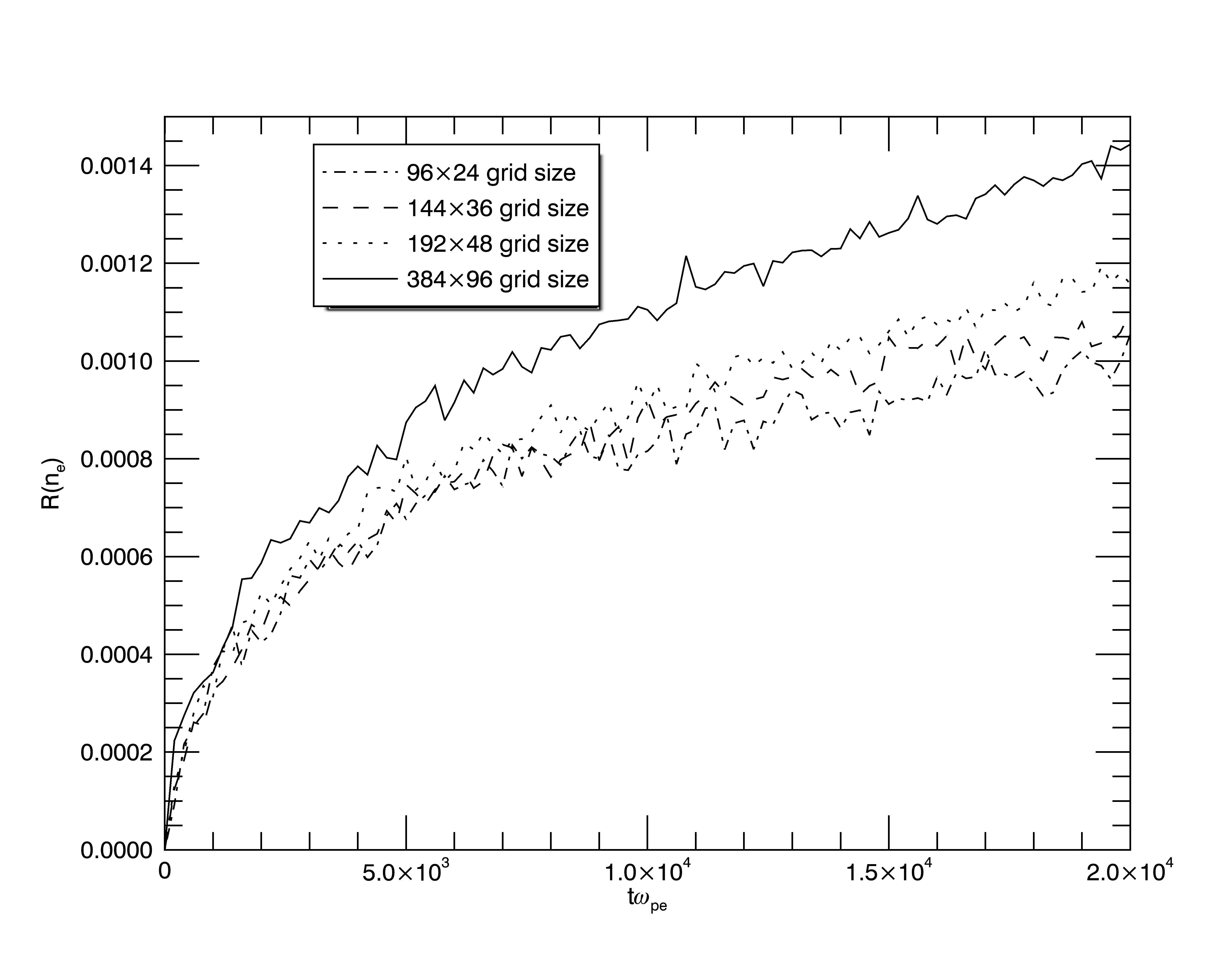
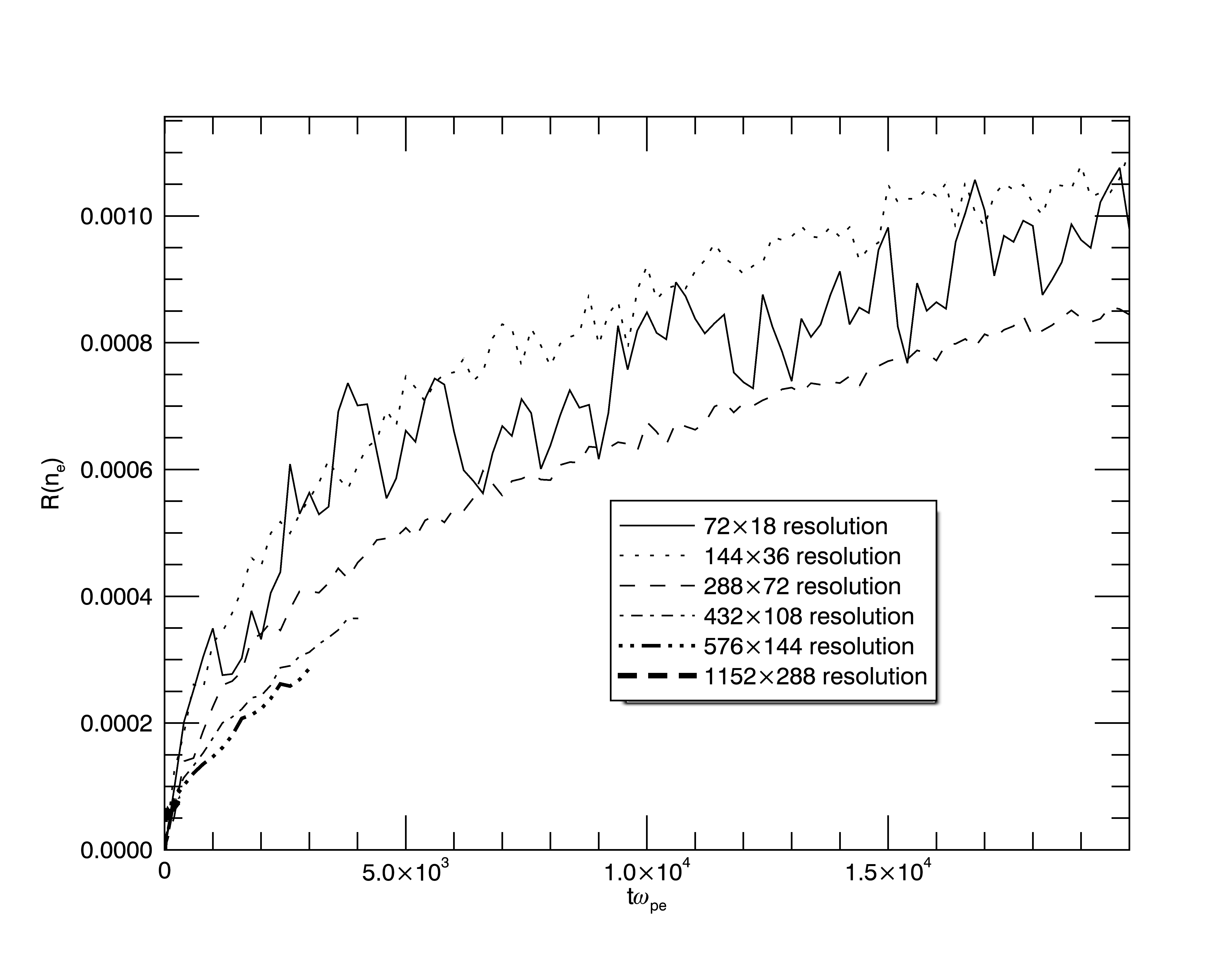
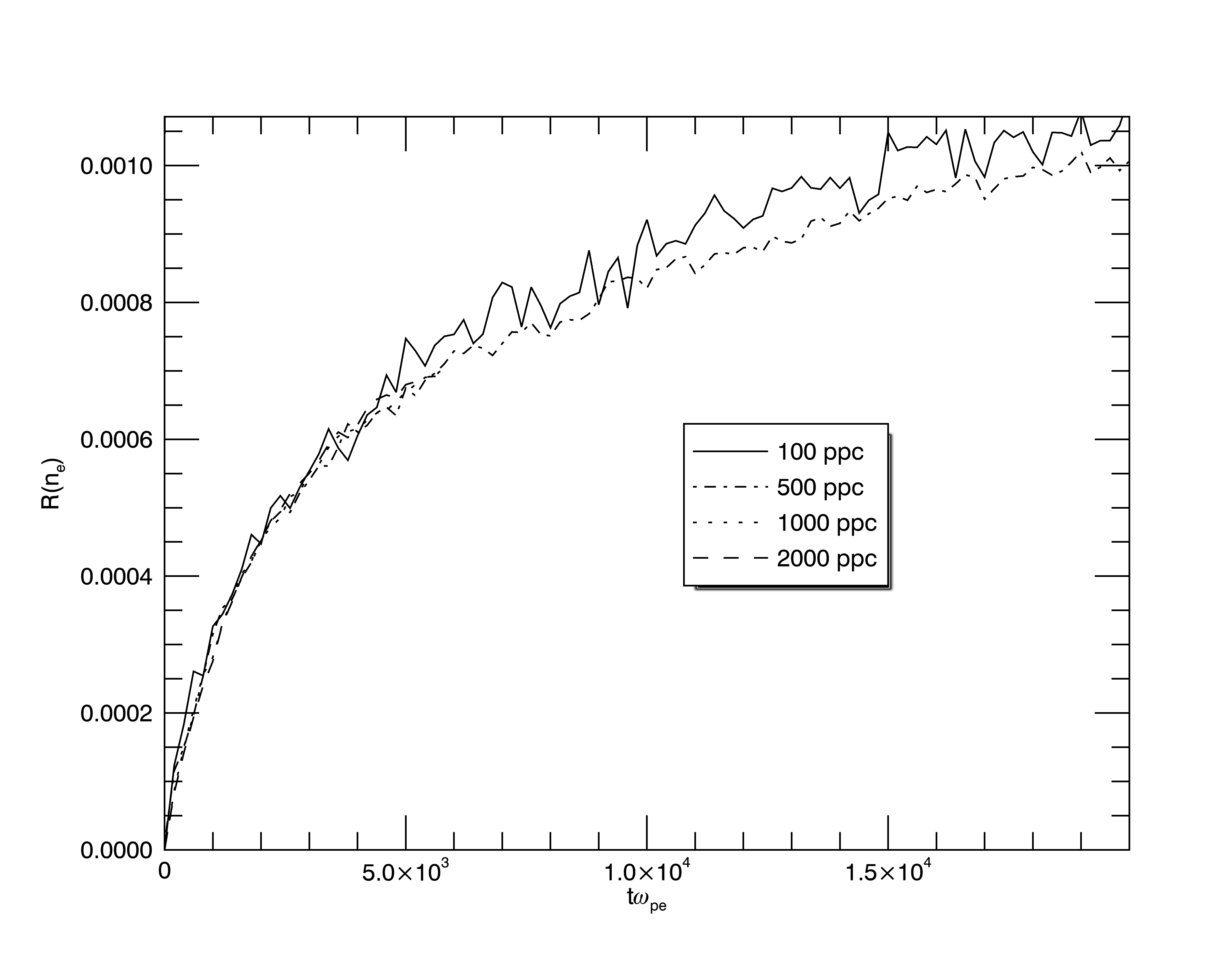
Figure 3: Top, mid and bottom panels show time evolution of $R(n_{e}(t))$ according to Eq.(1). The aim of this figure is to explore convergence of the numerical results as (i) domain size in top panel, (ii) grid resolution in mid panel and (iii) PPC in bottom panel are varied, accordingly.

Before presenting main results, it is important to make sure that the simulation results are not very sensitive with respect to the numerical parameters of the EPOCH model. This means that by altering (i) the computational domain size, (ii) the grid density, and (iii) the number of particles per cell (PPC) the obtained solutions remain reasonably unchanged.

We define the following quantity that is a physical measure of free charge creation by collisional ionization

$$R(n_{e}(t))=\frac{\int_{0}^{L_{x}}\int_{0}^{L_{y}}(n_{e}(x,y,t)-n_{e}(x,y,0))dxdy}{\sqrt{L_{x}L_{y}}\times\int_{0}^{L_{x}}\int_{0}^{L_{y}}n_{e}(x,y,0)dxdy},$$ (1)

where $n_{e}(x,y,t)$ is number density of electrons, $L_{x}$ and $L_{y}$ are grid lengths in x- and y- directions.

It can be noted that because of the normalisation by the initial (at $t=0$) number density of electrons, effectively, $R(n_{e}(t))$ gives percentage of electrons scaled by a scaling factor of $1/\sqrt{L_{x}L_{y}}$ to compare solutions obtained for different ensemble sizes corresponding to different numbers of identical computational cells. The scaling factor comes from considering the collision of particles in cells as a random process in terms of the interaction between different cells of the computational domain similar to the classical diffusion as discussed in the end of this sub-section.

For the numerical parameter sensitivity study, the case of $C60:C12$ fraction of $50:50$ is selected. For the numerical integration in Eq.(1) an Interactive Data Language’s (IDL’s) built-in function is used (INT_TABULATED). This function integrates a tabulated set of data $\{X_{i},F_{i}\}$ on the closed interval $\rm{[MIN(X),MAX(X)]}$, using a five-point Newton-Cotes integration formula. The implementation is based on introducing of an auxiliary array in EPOCH which contains y-array with x-values integrated out. This is followed by integration of the y-dependence in order to obtain a single value of $R(n_{e}(t))$ at a given solution time $t$.

The top, mid and bottom panels of Fig. 3 examine sensitivity of the numerical solution when gradually changing (i) the domain size, (ii) the grid resolution, and (iii) the PPC number. In the top panel of the figure, the grid unit is $\Delta=4\lambda_{D}$ and grid size is increasing by an appropriate factor e.g. $384\times 96$ for solid line. In the mid panel, the domain size remains the same, for example, our standard grid resolution $288\times 72$ has $\Delta=2\lambda_{D}$ while $432\times 108$ has $\Delta=(3/4)\lambda_{D}$, and commensurately $576\times 144$ has $\Delta=1\lambda_{D}$.

The bottom panel corresponds to the grid resolution of $144\times 36$ with $\Delta=4\lambda_{D}$ and varied PPC. This lower spatial resolution enabled us to access large PPC values while keeping the simulation cost feasible. It can also be noted that in Fig. 3 not all lines go up to the final dimensionless simulation time, this is because all numerical runs have been limited by 10 day (240 hour) wall-time. Typical numerical run utilized circa 144 processing cores connected with Infiniband Interconnect. In solutions presented on the mid and bottom panels in Fig. 3 the factor of $1/\sqrt{L_{x}L_{y}}$ from Eq.(1) correspond to different grid densities and varied numbers of particles per cell are. The solutions for four highest grid densities from the $288\times 72$ resolution and for all PPC numbers are in a good agreement with one another. The top fig. 3 shows that solutions for different domain sizes are in a reasonable agreement with the theoretical scaling depending on the statistical ensemble size.

All-in-all this confirms that the suggested simulation results are reasonably non-sensitive to the numerical parameters of the EPOCH model for the parameter range of interest. In all cases, the free charge created by collisional ionization as a function of time has the same functional behaviour which can be explained by a simple analytical linear model as discussed in the end of this sub-section.

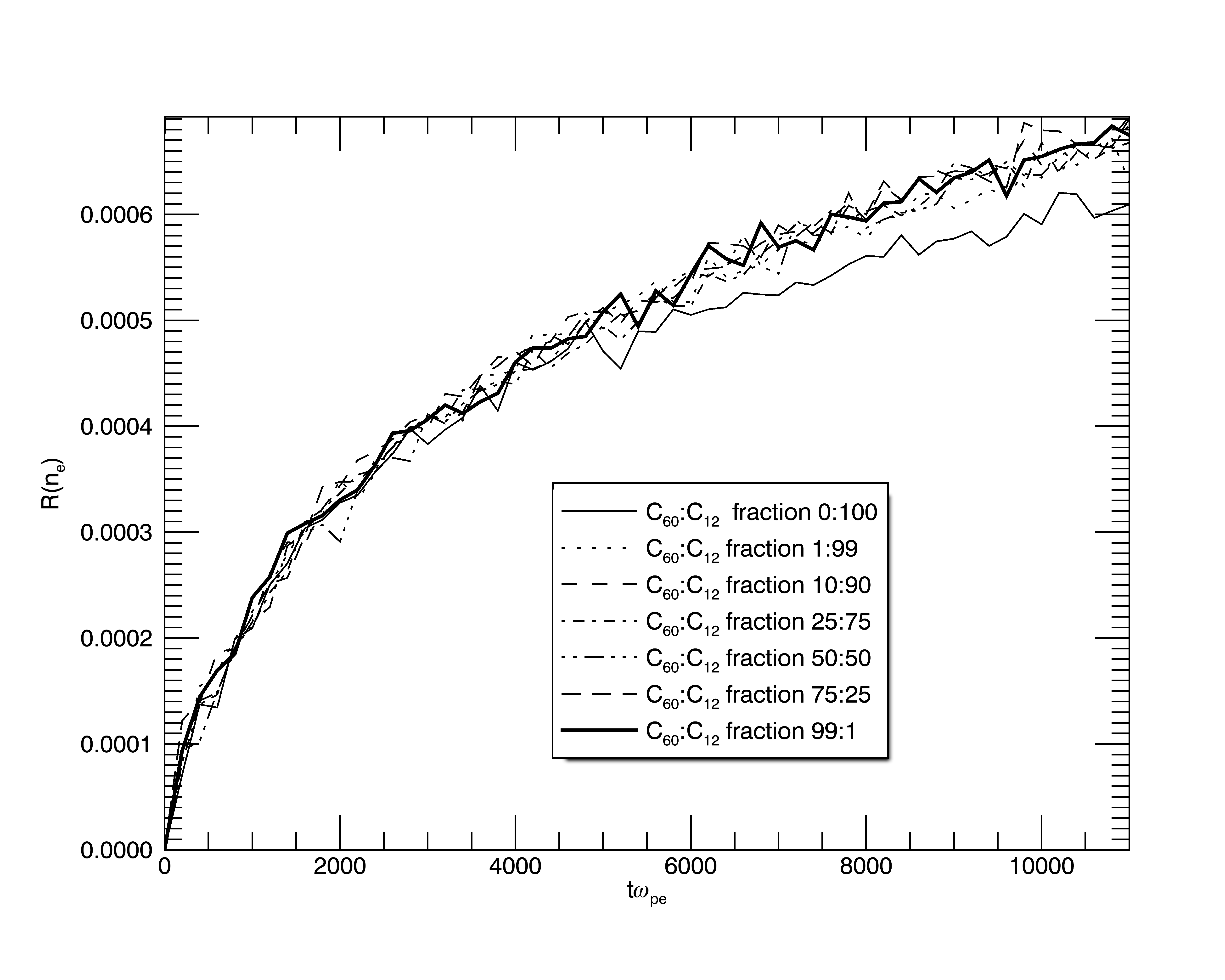
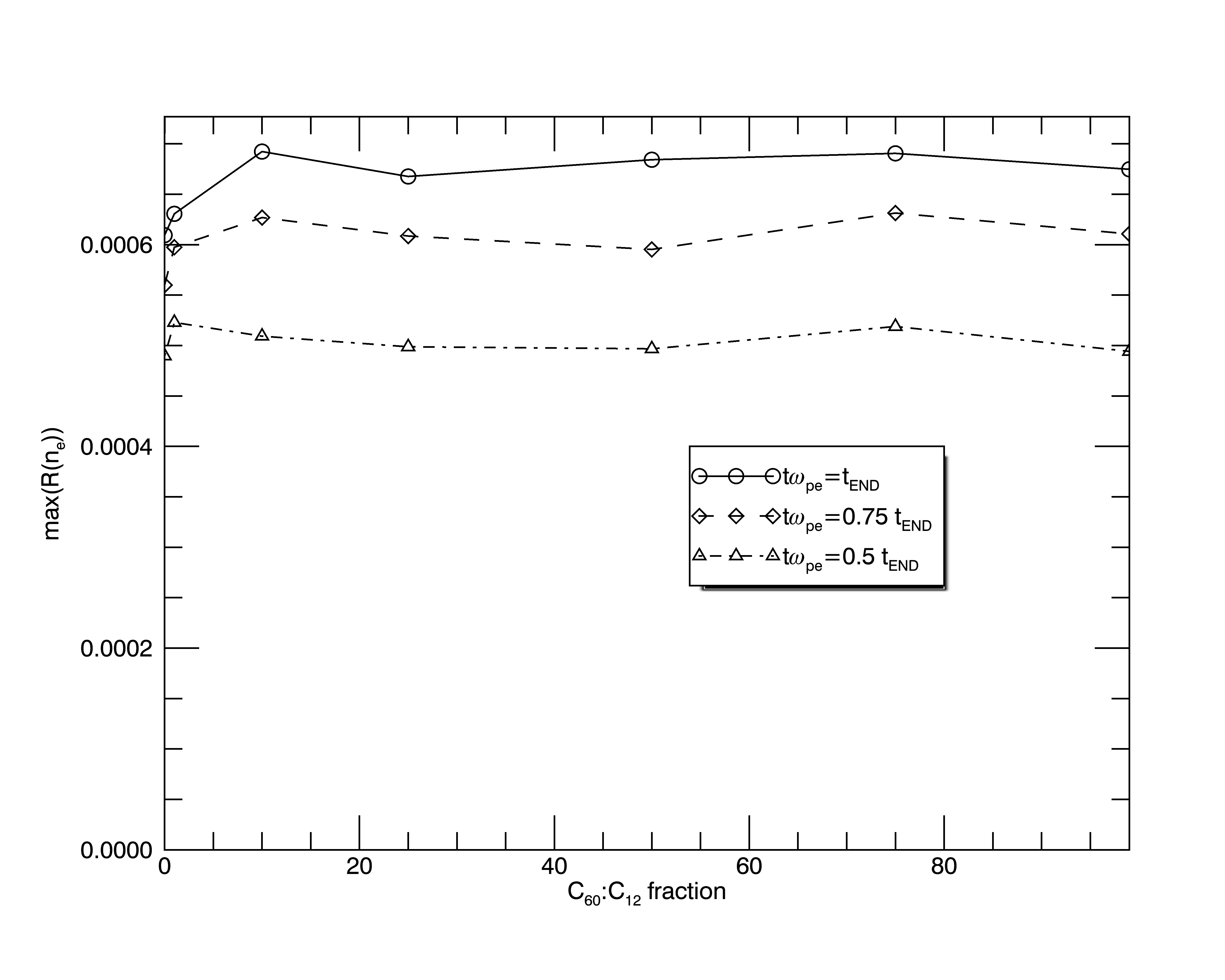
Figure 4: Top panel shows time evolution of $R(n_{e}(t))$, according to Eq.(1), for the different fractions: thin solid line is for $C60:C12$ fraction $0:100$, dotted line for $C60:C12$ fraction $1:99$, and so on, see panel inset for details, until thick solid line corresponding to $C60:C12$ fraction down to $99:1$. Bottom panel shows $R(n_{e}(t=t_{END}))$, i.e. $R(n_{e}(t)$ at the final simulation time with solid line with open circles, $R(n_{e}(t=0.75t_{END}))$ dashed line with open diamonds, $R(n_{e}(t=0.5t_{END}))$ dash-dotted line with open triangles.

In Fig. 4 we explore the effect of different $C60:C12$ fractions on free electron production. The fractions are as follows: $0:100$, $1:99$, $10:90$, $25:75$, $50:50$, $75:25$, $99:1$. Top panel shows time evolution of $R(n_{e}(t))$ for these different fractions. One important aspect immediately seen in this panel is that the absence of C60 yields smallest possible free electron production by collisional ionization. Even adding 1% of C60 markedly changes the situation. Bottom panel shows $R(n_{e}(t=t_{END}))$ solid line with open circles, $R(n_{e}(t=0.75t_{END}))$ dashed line with open diamonds, $R(n_{e}(t=0.5t_{END}))$ dash-dotted line with open triangles.

From the above results, a local optimum for free electron production by collisional ionization (i.e. a most efficient discharge condition) occurs for $C60:C12$ fraction of $10:90$. There is a second optimum in the flat part of the distribution which corresponds to $C60:C12$ fraction of about $80:20$. The bottom panel shows that the two optima are fairly persistent in the data once the simulation time becomes greater than $t=0.5t_{END}$.

Interestingly, the optimum corresponding to 10% of C60 is in a broad agreement with the preliminary experimental results of the Engineering Company Eco-Ardens who explored the efficiency of tribo-electric plasma generation in their gasifier for relatively small (less than 50%) fractions of C60 in the gas mixture.

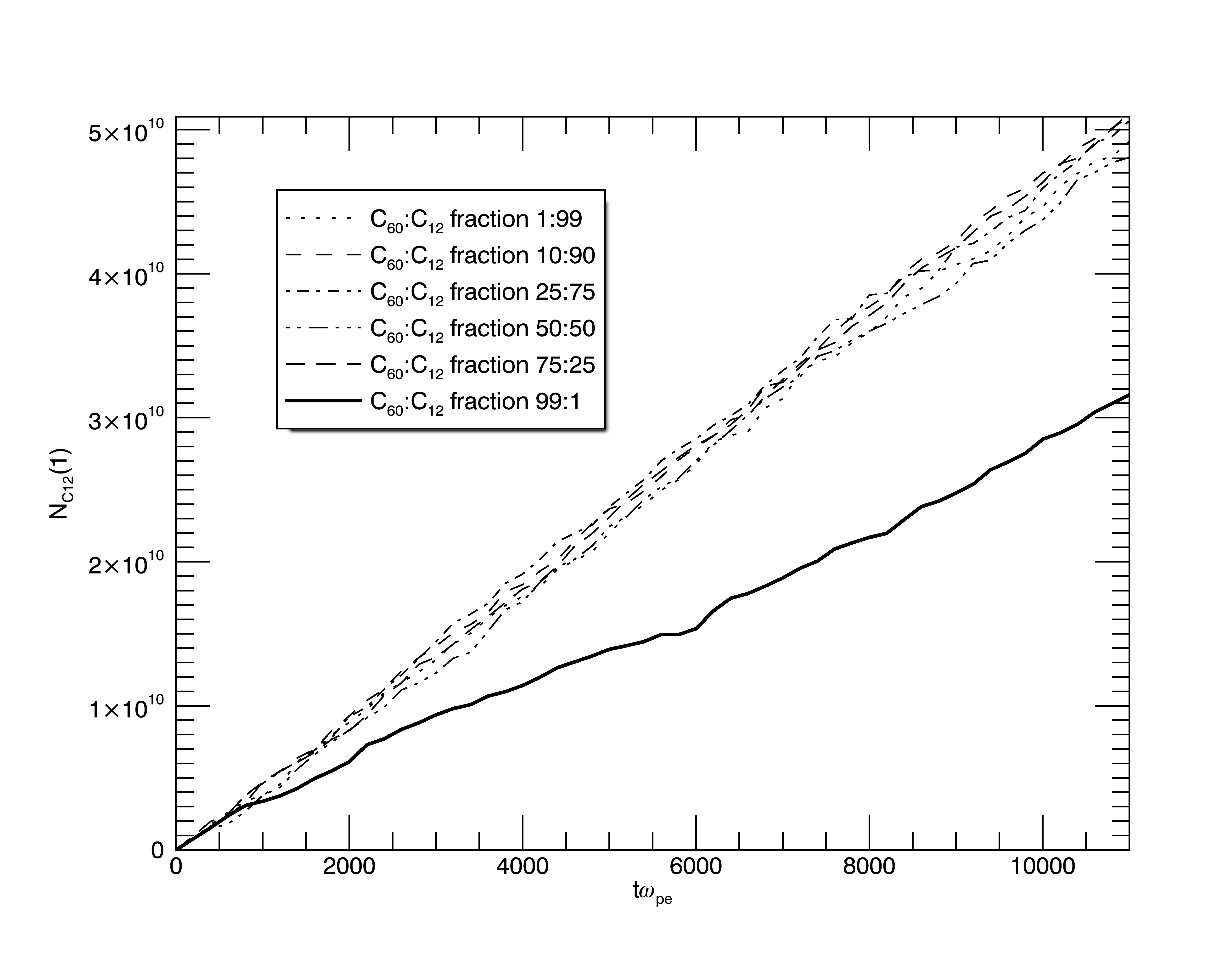
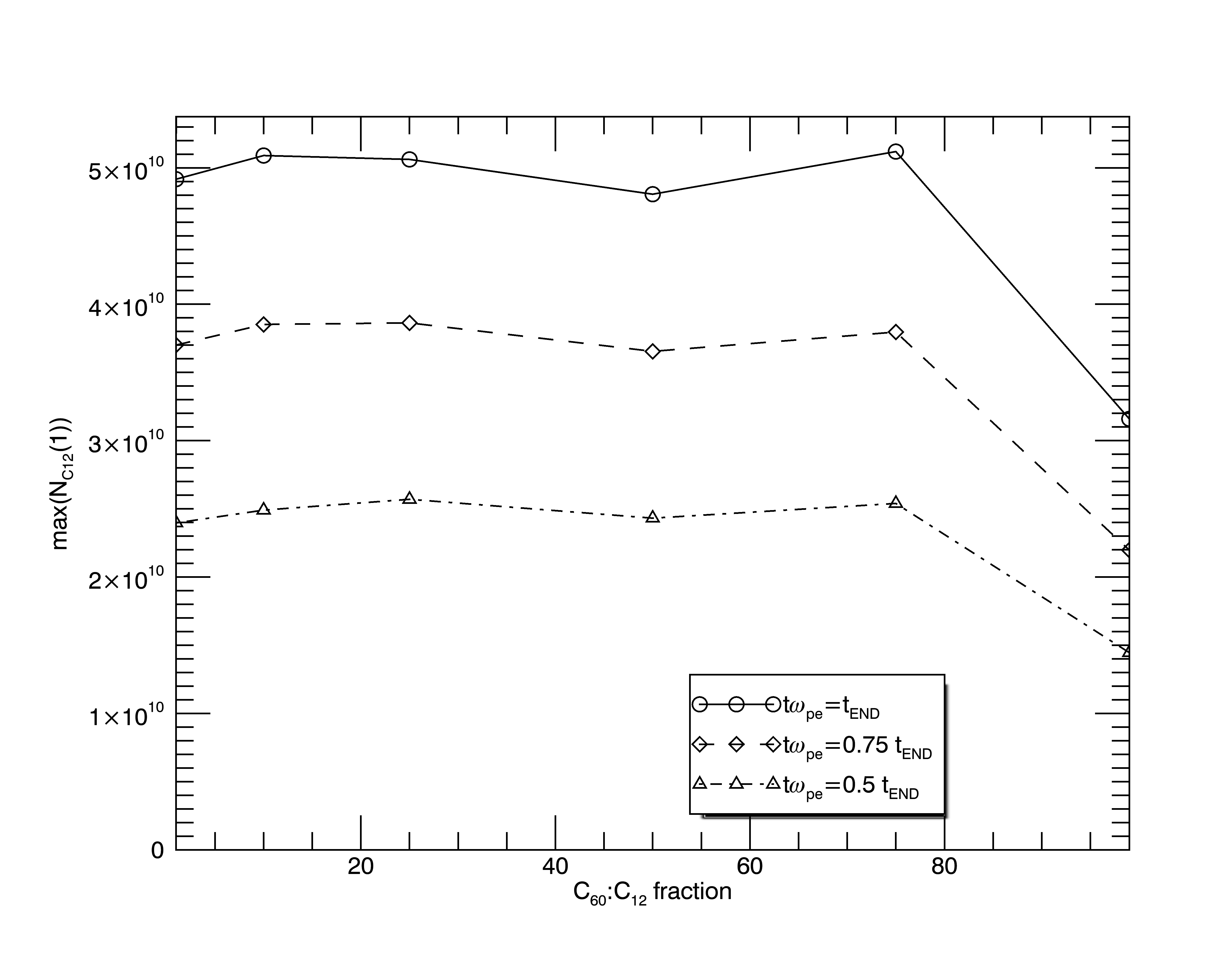
Figure 5: In the top panel we plot $N_{\rm C12}(1)(t)$, according to Eq.(2), for different $C60:C12$ fractions – see panel inset for details. In the bottom panel we plot $N_{\rm C12}(1)(t=t_{END})$ solid line with open circles, $N_{\rm C12}(1)(t=0.75t_{END})$ dashed line with open diamonds, $N_{\rm C12}(1)(t=0.5t_{END})$ dash-dotted line with open triangles.

Fig. 5 shows the effect of different $C60:C12$ fractions on C12+ (singly ionized C12) production by collisional ionization. In contrast to free electrons which are always present because of the background plasma field, there are no C12+ at $t=0$.

Hence, instead of a definition similar to Eq.(1) we quantify the C12+ production using

$$N_{\rm C12}(1)(t)=\frac{\int_{0}^{L_{x}}\int_{0}^{L_{y}}n_{\rm C12}(1)(x,y,t)dxdy}{\sqrt{L_{x}L_{y}}},$$ (2)

where $n_{\rm C12}(1)(x,y,t)$ is number density of C12+.

The top panel of Fig. 5, shows $N_{\rm C12}(1)(t)$ for different $C60:C12$ fractions. This quantity increases approximately linearly in time and different $C60:C12$ fractions have different growth rates. The difference of growth rates can be more readily seen in the bottom panel of Fig. 5 where we plot $N_{\rm C12}(1)(t=t_{END})$ solid line with open circles, $N_{\rm C12}(1)(t=0.75t_{END})$ dashed line with open diamonds, $N_{\rm C12}(1)(t=0.5t_{END})$ dash-dotted line with open triangles.

Similar to the free charge distribution (comp. with Fig. 4), there are the same two optima corresponding to $C60:C12$ fractions of $10:90$ and $80:20$. However, the first maximum ($C60:C12$ of $10:90$) is rather flat while the second peak is more prominent. The bottom fig. 4 shows that the broad and the sharp maxima are notable in the distribution for all solution times.

It should be noted that the values attained by $N_{\rm C12}(1)$ are much smaller than the number density of electrons in the plasma $n_{e}$ as well as the number of free electrons generated by collisions. For example, by making the following substitution $n_{\rm C12}(1)(x,y,t)\to n_{e}(x,y,t)$ in Eq.(1) for $C60:C12$ fraction of $10:90$ and taking $t=t_{END}$, it follows that $N_{\rm n_{e}}(t=t_{END})=1.98\times 10^{14}$ which gives the number of generated free electrons. By comparison with the maximum value of $N_{\rm C12}$ (shown in the top panel of fig. 5), the number of free electrons generated by collisions is three orders of magnitude larger.

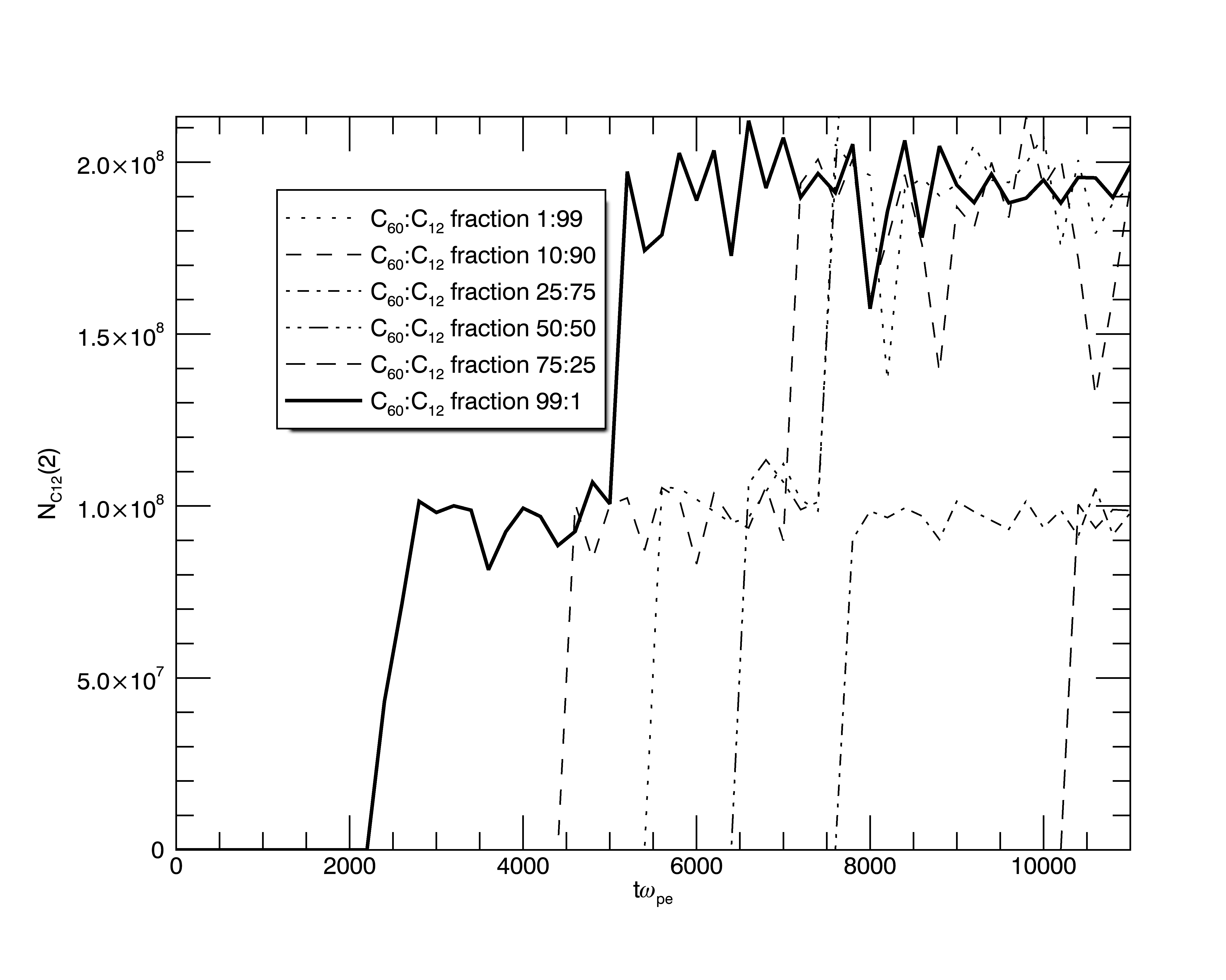
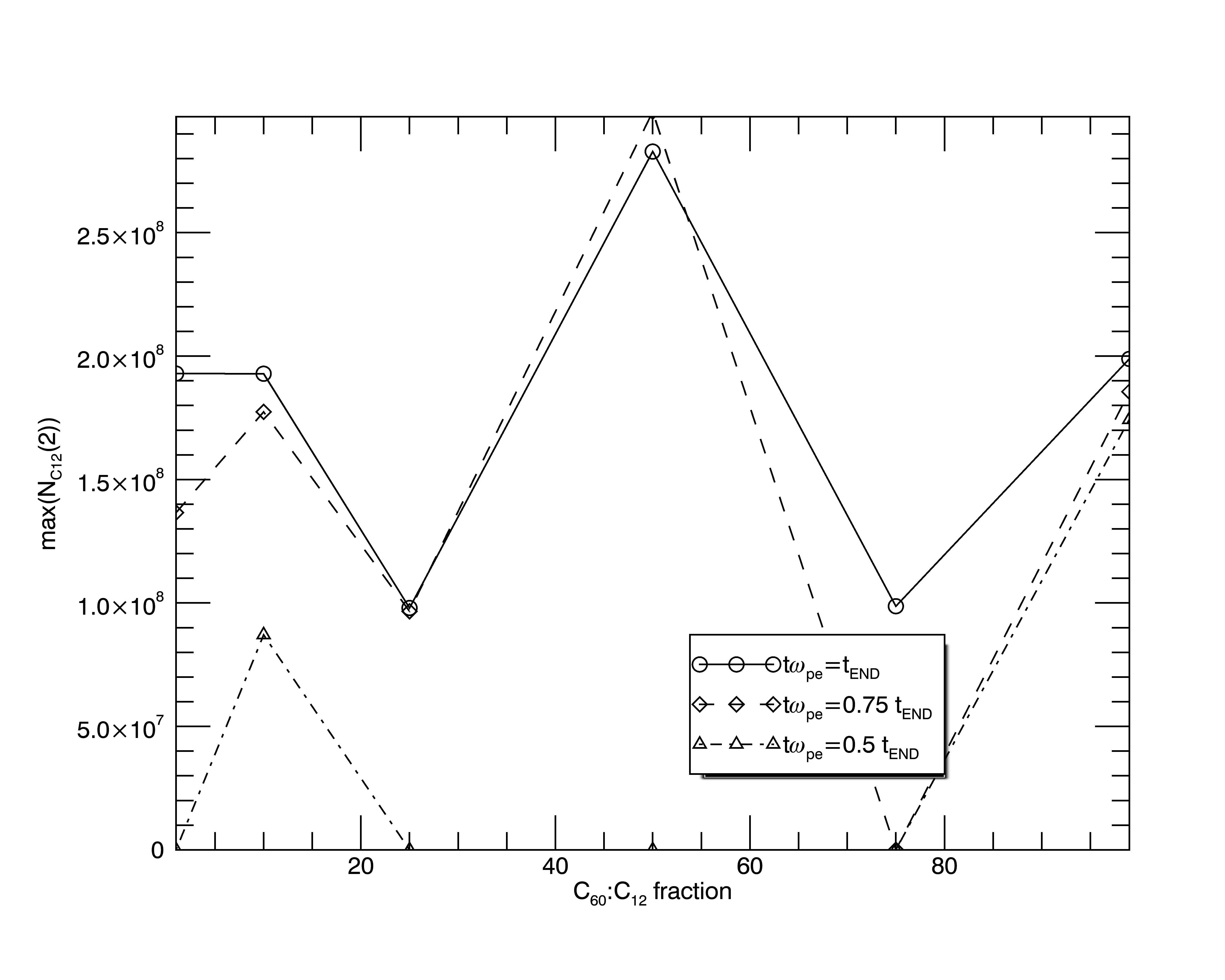
Figure 6: Time evolution of $N_{\rm C12}(2)(t)$, defined by Eq.(2), as in Fig.5, but replacing $n_{\rm C12}(1)(x,y,t)$ now with $n_{\rm C12}(2)(x,y,t)$, the latter being number density of C12++. Here, as in Fig.5, we study of the effect of different $C60:C12$ fractions on C12++ (doubly ionized C12) production by collisional ionization – see panel insets for details.

Fig. 6 demonstrates the effect of different $C60:C12$ fractions on C12++ (doubly ionized C12) production by collisional ionization. $N_{\rm C12}(2)(t)$ is defined as by Eq.(2) but simply replacing $n_{\rm C12}(1)(x,y,t)$ by $n_{\rm C12}(2)(x,y,t)$ with the latter being number density of C12++. Two observations follow from top panel Fig. 6: (i) there is no longer monotonous increase of C12++ production by collisional ionization. Instead, the process proceeds in jumps. For example, for the case of $C60:C12$ fraction of $10:90$, represented by a dashed line, there are two jumps at $t\omega_{pe}=4500$ and $6500$. (ii) the obtained number densities of C12++ are further three order of magnitude smaller in comparison with the singly ionized C12 case, e.g. $N_{\rm C12}(2)(t=t_{END})=2\times 10^{8}$ for most cases. (iii) there are three peaks in the number density distribution of C12++ as a function of the $C60:C12$ fraction. In addition to $C60:C12$ fraction of $10:90$, two new maxima include $C60:C12$ fraction of $50:50$ and another peak at high fullerene concentrations tending to $100:0$.

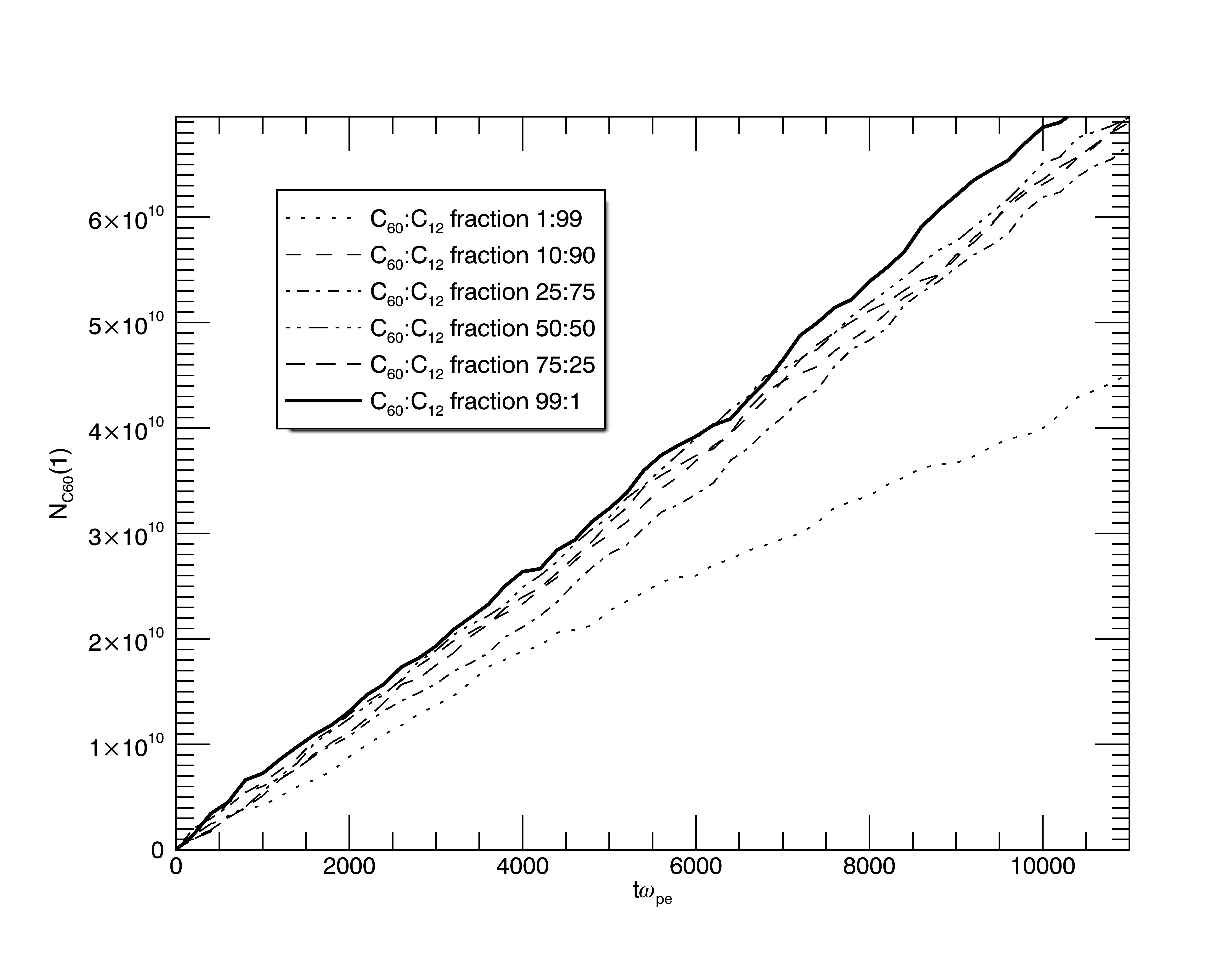
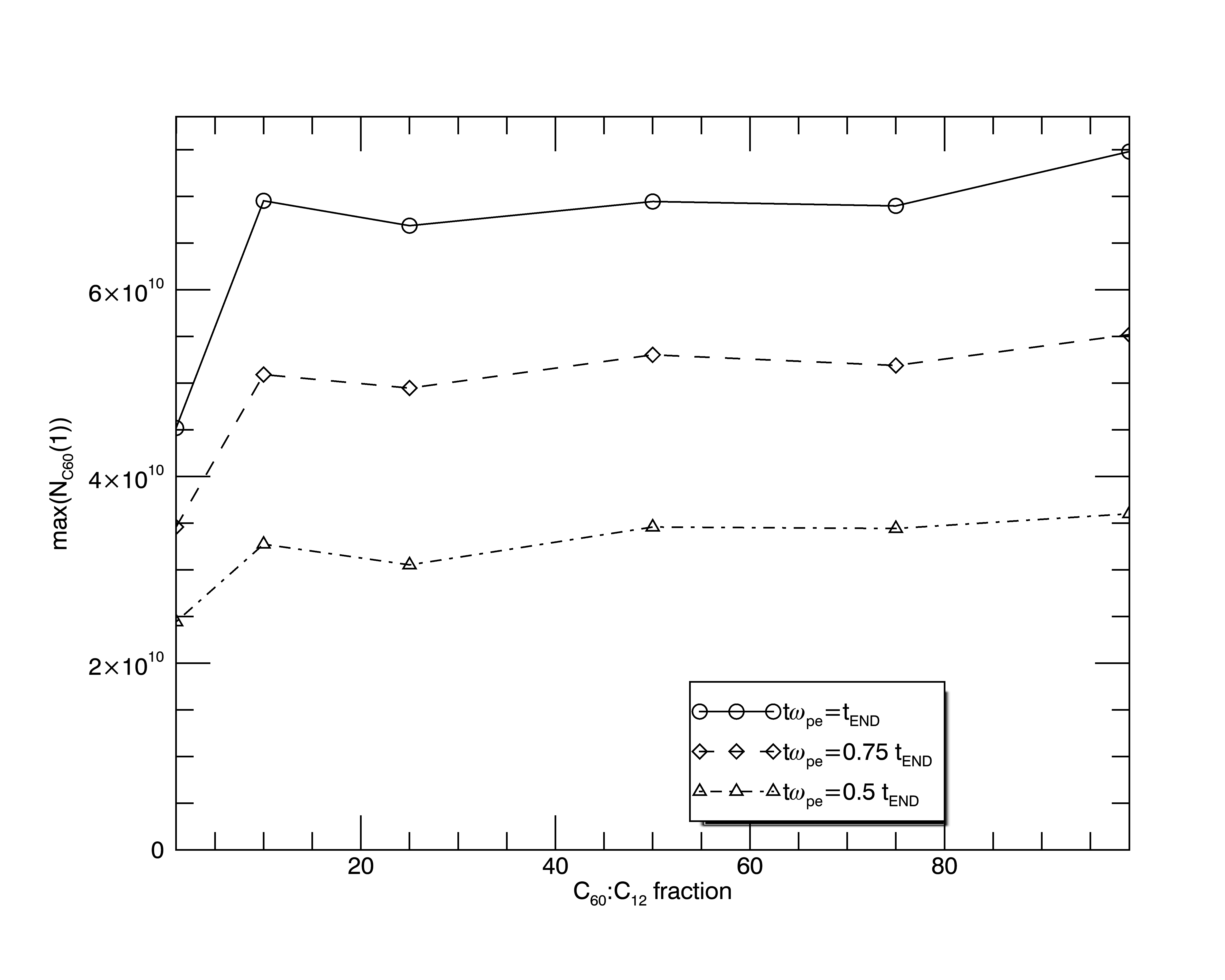
Figure 7: As in Fig. 5, but now investigating the effect of different $C60:C12$ fractions on C60+ (singly ionized C60, i.e. fullerene) production by collisional ionization.

Fig. 7 shows the effect of different $C60:C12$ fractions on C60+ (singly ionized C60, i.e. fullerene) production by collisional ionization. Broadly speaking, the behaviour of C60+ is similar to that on of C12+ shown in Fig. 5, except for: (i) the number density values of C60+ is about 30% larger in comparison with that of C12+ and (ii) the peak at $C60:C12$ fraction of $10:90$ is more clearly pronounced and the broad peak at high fractions of $C60:C12$ moves to $100:0$.

To conclude this section, an analytical ionization model is considered where the C12 and C60 species are lumped together as the two-species (ionised and non-ionised) of a particle gas immersed in plasma. Following ref.Draine (2011), by introducing constant ionization and recombination parameters $\alpha=const>0$ and $\beta=const>0$, assuming that the number of electrons per unit volume is approximately constant, $n_{e}=const>0$ (i.e. the change of the electron number density due to ionization is much smaller in comparison with the original electron number density in plasma, $n_{e}(t)/n_{e}(0)\approx 1$), and denoting the numbers of ionized and non-ionized particles by $n_{1}$ and $n_{2}$, respectively, so that $n_{1}+n_{2}=n_{0}=const>0$, where $n_{0}$ is the total number of particles per unit volume that is fixed constant, the evolutionary equation for the ionized particles is given by:

$$\frac{\partial n_{1}}{\partial t}=\alpha n_{e}n_{2}-\beta n_{e}n_{1}.$$ (3)

Equation (3) is solved in a periodic spatial domain $0\leq x\leq L_{x}$, and $0\leq y\leq L_{y}$ with the initial condition: $n_{1}(x,y,0)=0$ and under the constraint that $n_{1}+n_{2}=n_{0}$.

From integration of Eq.(3) over the control volume $V=\int_{0}^{L_{x}}\int_{0}^{L_{y}}dxdy$ one obtains:

$$\frac{d\langle n_{1}\rangle}{dt}=\alpha N_{e}\langle n_{2}\rangle-\beta N_{e}\langle n_{1}\rangle,$$ (4)

where $\langle f\rangle=\int_{0}^{L_{x}}\int_{0}^{L_{y}}fdxdy$. The constraint after averaging yields $\langle n_{2}\rangle=\langle n_{0}\rangle-\langle n_{1}\rangle$, which is then substituted into Eq. (4) to obtain

$$\frac{d\langle n_{1}\rangle}{dt}=\alpha N_{e}\langle n_{0}\rangle-(\beta+\alpha)N_{e}\langle n_{1}\rangle,$$ (5)

where $N_{e}$ is the electron number in the considered control volume $V$assuming that the non-linear process in the bigger volume leads to an appropriate renormalisation of the coefficients $\alpha$ and $\beta$. By introducing new notations $\langle n_{i}\rangle=\langle n_{1}\rangle/\langle n_{0}\rangle$, $a=(\alpha+\beta)N_{e}$ and $b=\alpha/(\alpha+\beta)$ Eq.(5) simplifies to

$$\frac{d\langle n_{i}\rangle}{dt}=-a(\langle n_{i}\rangle-b).$$ (6)

Using the initial condition, the solution for the averaged particle number in the control volume $V$ is

$$\langle n_{i}\rangle(t)=b\left(1-\exp(-at)\right).$$ (7)

The above analytical solution can be compared with predictions of the relative change in electron number density computed using EPOCH code, $R(n_{e})=\left(\langle n_{e}(t)\rangle-\langle n_{e}(0)\rangle\right)/\langle n_{e}(0)\rangle$, which essentially coincides with our definition for $R(n_{e})$ from Eq.(1). First of all, note that the number of ionized particles scales with the number of new electrons generated such that

$$\langle n_{i}\rangle=C\left(\langle n_{e}(t)\rangle-\langle n_{e}(0)\rangle\right)/\langle n_{e}(0)\rangle,$$ (8)

where $C=const>0$. Hence, $\ln(\langle n_{i}\rangle)=\ln(R(n_{e}))+\ln(C)$ and, using Eq.(7)

$$\frac{d\ln(R(n_{e}))}{dt}=\frac{d\ln(\langle n_{i}\rangle)}{dt}=\frac{a}{1-\exp(-at)}.$$ (9)

For initial times $at\ll 1$, Eq.(9) can be further simplified using the Taylor expansion that leads to the asymptotic solution as follows

$$\frac{d\ln(R(n_{e}))}{dt}\simeq\frac{1}{t}.$$ (10)

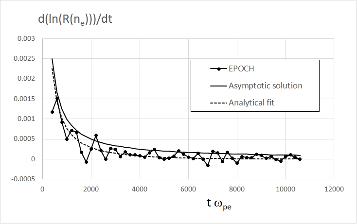
Figure 8: Solution of the homogeneous particle ionization problem: comparison of the EPOCH solution (solid line with dots) with the analytical solutions, where solid line shows asymptotic solution according to Eq.(10) and dashed line is analytical solution, according to Eq.(9), in which the value of parameter $a$ has been adjusted to obtain the best fit with the EPOCH solution.

Fig. 8 shows comparison of the EPOCH solution with the analytical solution Eq. (9) and the asymptotic solution Eq. (10). In the case of the analytical model Eq. (9), the value of parameter $a$ has been adjusted to obtain the best fit with the EPOCH solution.

It can be noted that, despite some noise present in the EPOCH data due to the numerical differentiation, the analytical solutions based on Eqs.(9) and especially (10) are in a good agreement with the numerical solution.

By recalling the need to explain the scale-factor of $1/\sqrt{L_{x}L_{y}}$ from Eq.(1) mentioned when we discussing top panel Fig. 3, we next explore the effect of the periodic boundary condition for comparison of the simulation results in different domain sizes.

Let us consider the solution of Eq. (5) in a large domain, $V^{N,M}=\int_{0}^{N\times L}\int_{0}^{M\times H}dxdy$, where $N,M>1$ are the total number of grid cells and the x- and the y- direction, respectively. The control volume $V$, considered in the previous analysis can be treated as subset of the large domain. The goal is to compare the particle number density solution, Eq. (7), obtained in the domain $V$ and the same averaged over the larger domain $V^{N,M}$. To proceed, the large domain is broken down in several over non-overlapping sub-volumes $V^{k,l}=\int_{k\times L}^{(k+1)\times L}\int_{l\times H}^{(l+1)\times H}dxdy$, where $1<k<N$ and $1<l<M$. Each of these sub-volumes $V^{k,l}$ is equal to $V$ but, in comparison with the single volume case, the particle collision processes in separate sub-volumes are largely uncorrelated with one another. The particle numbers averaged over each sub-volume $V^{k,l}$ satisfy to Eq(6). Each of these quantities can be treated as random variables, whose evolutionary equations can be treated by analogy with the Langevin diffusion

$$\frac{dn_{i}}{dt}=-an_{i}+\{R\},$$ (11)

where $\{R\}=ab$ is the generation term that can be interpreted as a random force and brackets of the volume averaging in the particle number variable are omitted. Here $a=(\alpha+\beta)N_{e}$, where $N_{e}$ is the electron number corresponding to the large domain ensemble. In accordance with the well-known solution of the Langevin equation van Kampen (2003), the variance of the ensemble averaged number of the particles grows as

$$\langle n_{i}^{2}\rangle(t)=\left[\langle n_{i}^{2}\rangle(0)-Amp(R)^{2}/(2a)\right]\exp(-2at)$$

$$+Amp(R)^{2}/(2a),$$ (12)

where $Amp(R)=ab$. Hence,

$$\left(\langle n_{i}(t)\rangle-\langle n_{i}(0)\rangle\right)\simeq\sqrt{\langle(n_{i}^{2}(t)\rangle}=$$

$$\sqrt{\left[\langle n_{i}^{2}\rangle(0)-ab^{2}/2\right]\exp(-2at)+ab^{2}/2}.$$ (13)

At equilibrium, $\left(\langle n_{i}(t)\rangle-\langle n_{i}(0)\rangle\right)=\sqrt{a/2}b=\sqrt{N_{e}/2}\frac{\alpha}{(\alpha+\beta)}$ and the quantity $\left(\langle n_{i}(t)\rangle-\langle n_{i}(0)\rangle\right)/\sqrt{N_{e}}=\sqrt{\frac{\alpha}{2(\alpha+\beta)}}$ should be independent of the size of the considered system, $\simeq NM$. Using Eq.(8) this leads to the following scaling of the simulation results for different size periodic domains:

$$R(n_{e})/\sqrt{N_{e}}=const$$ (14)

The top panel Fig. 3 shows the simulation results for different domain sizes. It can be noted that the revealed dependency of the ionized particle solution on the domain size is similar to the so-called ”shot noise” effect reported in the start-up laser problems Freund et al. (2008). Because (i) $N_{e}\propto NM\propto L_{x}L_{y}$ and (ii) all lines for the different domain sizes in top panel of Fig. 3 are tolerably close to each other, hence scale-factor of $1/\sqrt{L_{x}L_{y}}$ from Eq.(1) is justified based on our Langevin equation solution.

II.3 Particle interaction with including the non-homogenous wall condition

The EPOCH results describing how surface roughness affects free charge generation by collisional ionization are presented next. Instead of including actual material rough walls in the simulation, computationally, it is much easier to impose periodic electric field on the domain boundary. Indeed, rough surfaces alter electric field in the vicinity of the solid boundaries and the imposition of a non-uniform electric field boundary condition along with the periodic condition on particles is equivalent to considering a small internal volume of the particle domain at some distance away from the material walls. It can be reminded that enforcing of the periodic condition is important for consistency with the Maxwell’s equations.

In EPOCH code, the boundary condition on the electric and magnetic field dynamics is implemented via a subroutine called fields.f90, see for details ref.Arber et al. (2015). The following target electric fields at $y=y_{\rm min}=1$ are considered ($x$ is tangential to the wall boundary and $y$ is the normal direction):

(i) $E_{y}(x,t)=f(x,t)$ and (ii) $E_{x}(x,t)=f(x,t)$, where

$$f(x,t)=E_{0}\times\biggl{(}\exp(-(x-0.2x_{\rm max})^{6}/(x_{\rm max}/15)^{6})+$$

$$\exp(-(x-0.4x_{\rm max})^{6}/(x_{\rm max}/15)^{6})+$$

$$\exp(-(x-0.6x_{\rm max})^{6}/(x_{\rm max}/15)^{6})+$$

$$\exp(-(x-0.8x_{\rm max})^{6}/(x_{\rm max}/15)^{6})\biggr{)}$$

$$\times\left[1.0-\exp\left(-t/(10/\omega_{pe})\right)\right],$$ (15)

and where $E_{0}=10^{7}$ Vm^-1.

The boundary condition at $y=y_{\rm min}=1$ is driven to the target field Eq(15) so that in about $t\omega_{pe}=10$ a steady state electric field with an amplitude of $E_{0}$ is reached. Such driving essentially imposes a comb-like electric field with four spikes at locations of $0.2,0.4,0.6,0.8$ fraction of the computational domain size in the x-direction.

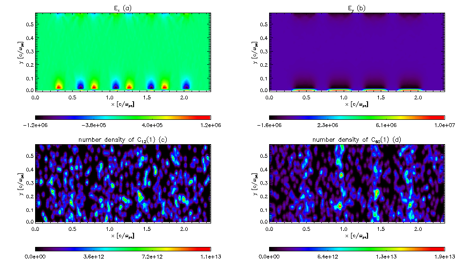
Figure 9: Top panels (a) and (b) show electric field x- and y- components, respectively, while bottom panels (c) and (d) should number densities of C12+ and C60+ at final simulation time $t\omega_{pe}=20000$, respectively. The data is for driving the electric field component normal to the boundary.

Fig. 9 shows simulation results for the case of electric field component normal to the boundary. The top panels demonstrate electric field x- and y- components, and bottom panels show number densities of C12+ (singly ionized C12) and C60+ (singly ionized C60) at final simulation time $t\omega_{pe}=20000$. The length scale units are based on the plasma frequency and the light speed.

In the top panels of Fig. 9, the electric field gradients are very localised and moderately penetrate in the domain interior. The ’hot spots’ which emerge in the two bottom panels of Fig. 9 represent charged ions of the relevant species. These species are relatively rare and more-or-less scattered over the whole domain.

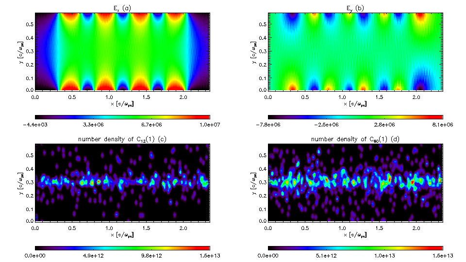
Figure 10: The same as in Fig.9 but for the case of the electric field tangential to the wall boundary

Fig. 10 shows simulation results for the case of tangential to x-direction electric field. The top panels show electric field x- and y- components, and bottom panels should number densities of C12+ and C60+ at final simulation time $t\omega_{pe}=20000$. Two important observations from Fig. 10 include: (i) $E_{x}$ now protrudes into the simulation domain much deeper than in the case of normal electric field driving and the ’flames’ of the electric field gradient are much wider; (ii) the ’hot spots’ of C12+ and C60+ are clustered in the middle of the simulation domain at $y=y_{\rm max}/2$.

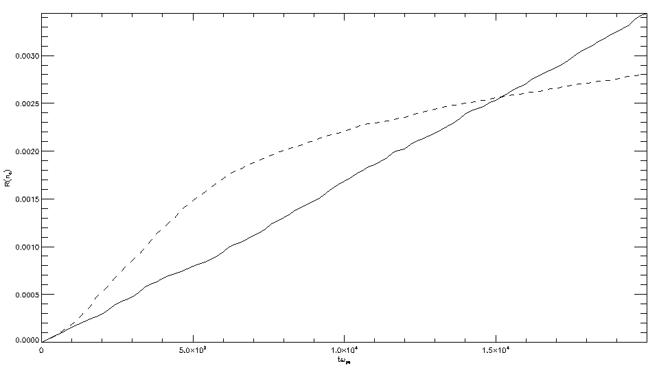
Figure 11: $R(n_{e})$ for the normal and tangential electric field driving cases. Solid line is for the case of normal and dashed for the case of tangential electric field driving.

Fig. 11 compares the time evolution of the previously defined relative integral charge, $R(n_{e})$ that was generated in the case of the normal and the tangential electric field boundary condition. Solid line is for the case of normal and dashed for the case of tangential electric field driving. For the normal electric field case, the generated free charge, $R(n_{e})$ shows an approximately linear behavior without a sign of saturation. The suggests that the end simulation time has not been long enough to reach a quasi-steady state in this case. However, in the case of the tangential electric field, the accumulated charge curve shows a sign of exponential stagnation towards a saturated state in accordance with the linear collision model discussed in the previous section.

Importantly, the charge localisation effect triggered by the tangential electric field boundary condition means that additional carbon particles, which could be introduced in the ’reaction zone’ in the centre of the computational domain, would further enhance collisional discharges and lead to a denser tribo-electrically created plasma. Indeed, the charge localisation effect is the tribolectric plasma generation scenario as suggested by the Engineering Company Eco-Ardens experimental results (comp. with Fig.2). In these experiments, the additional carbon particles were brought in the tribo-plasma reaction zone by pyrolysis products. In comparison with the tangential electric field boundary condition, the normal electric field has no significant effect on the localisation of particle charging. Hence, at least for the simulation run times attempted in this study, this other regime is not of interest from the point of view of tribo-electric plasma generation. The rest of the section describes an analytical model for the stationary localised distribution of free charge accumulation in the case of the tangential electric field boundary condition.

Let us consider a two dimensional domain with periodic boundary conditions in the x- and y-direction. In comparison with the model considered in the previous section, in the present case the boundary problem is not homogeneous: the top and the bottom boundaries in the y-direction correspond to conducting walls. On the walls, a periodic variation of the tangential electric field component is imposed, $E_{x}=E_{x}(x)$. In accordance with the EPOCH solution (Fig. 10), the electric field penetrates inside the domain and its effect decays away from the wall. To proceed with the analytical solution, let us model the effect of the non-homogeneous electric field on the ionized particle distribution by adding a diffusion term to the linear particle collision model equation (3). At equilibrium $\partial n_{1}/\partial t=0$ and the equation for the particle number per unit volume becomes

$$\alpha n_{e}n_{2}-\beta n_{e}n_{1}+D\frac{\partial^{2}n_{1}}{\partial y^{2}}=0,$$ (16)

where $D=const>0$. Let us discretise the solution domain into several non-overlapping bins in the y-direction where the coordinates of each bin are $0\leq x\leq L_{x},\,\,\,h\leq y\leq h+\delta h,\,\,\,0<h<L_{y}.$ By integrating Eq.(16) over each bin volume, one obtains

$$\alpha N_{e}\langle n_{2}\rangle-\beta N_{e}\langle n_{1}\rangle+\langle D\frac{\partial^{2}n_{1}}{\partial y^{2}}\rangle=0,$$ (17)

where the brackets mean averaging over the bin volume. After a re-arrangement, using $n_{1}+n_{2}=n_{0}$ and $\langle n_{i}\rangle=\langle n_{1}\rangle/\langle n_{0}\rangle$, $a=(\alpha+\beta)N_{e}$ and $b=\alpha/(\alpha+\beta)$, Eq(17) reduces to

$$\langle D\frac{d^{2}n_{i}}{dy^{2}}\rangle=a\left(\langle n_{i}\rangle-b\right).$$ (18)

By introducing some effective average diffusion coefficient $\bar{D}$, the last equation can be integrated to obtain

$$\langle n_{i}\rangle=b+A\exp\left(\sqrt{\frac{a}{\bar{D}}}y\right),$$ (19)

where $A=const$ is an amplitude parameter to be determined, e.g. from the boundary condition.

At small distances from the bottom wall, $\sqrt{\frac{a}{\bar{D}}}y\ll 1$, Eq. (19) reduces to integrated to obtain

$$\langle n_{i}\rangle=C+Ey,$$ (20)

where $C=b=const$ and $E=A(1+\sqrt{\frac{a}{\bar{D}}})=const$.

To close the model, the slope parameter $E$ in Eq.(20) can be related to the tangential electric field using the particle continuity and the electrostatic force equations as follows. Let us consider the continuity equation for the number of ionized particles in a unit volume at equilibrium:

$$\frac{\partial\left(u_{x}n_{i}\right)}{\partial x}+\frac{\partial\left(u_{y}n_{i}\right)}{\partial y}=0.$$ (21)

Here $u_{x}$ and $u_{y}$ are effective x- and y- velocity components. The particle velocities are driven by the non-homogeneous electric field. By integrating Eq. (21) over the considered control volume close to the wall, to the first order, one obtains

$$\frac{d\langle n_{i}\rangle}{dy}\approx-\langle n_{i}\rangle_{y=0}{\langle\frac{\partial\left(u_{x}\right)}{\partial x}\rangle}/{U}.$$ (22)

Eq.(22) can be reduced to the form of Eq.(20), where brackets correspond to the volume averaging and $E=-\langle n_{i}\rangle_{y=0}{\langle\frac{\partial\left(u_{x}\right)}{\partial x}\rangle}/{U}$, which can be treated as constant to the first approximation. Let us further approximate the particle velocity corresponding to their drift away from the wall by a constant value, $u_{y}=U>0$ and take into account that the average number of particles does not depend on the x-coordinate. To evaluate ${\langle\frac{\partial\left(u_{x}\right)}{\partial x}\rangle}$ that appears as the slope, $E$, one can recall that the acceleration exerted on a charged particle due to the electric field is given by

$$a_{x}(x,y)=qE_{x}(x,y)/m$$ (23)

where $q$ is the particle charge and $m$ is its mass, and using the standard kinematic relationships,

$$u_{x}=\int_{0}^{t}a_{x}(x,y)dt=\int_{0}^{x}\frac{a_{x}(x,y)}{u}dx\,\,\,{\rm and}\,\,\,u\frac{\partial u}{\partial x}=a_{x}(x),$$ (24)

the integration over $[0,x]$, after some re-arrangement, leads to

$$u_{x}(x,y)=\sqrt{\int_{0}^{x}{a_{x}(x,y)}dx+u_{x}^{2}(0,y)}.$$ (25)

Hence,

$$\langle\frac{du_{x}}{dx}\rangle=\frac{1}{2}\langle\frac{a_{x}(x,y)-a_{x}(0,y)}{\sqrt{\int_{0}^{x}{a_{x}(x,y)}dx+u^{2}(0,y)}}\rangle,$$ (26)

or

$$\langle\frac{du_{x}}{dx}\rangle=\frac{q}{2m}\langle\frac{\Delta E_{x}}{\sqrt{\int_{0}^{x}{(q/m)E_{x}(x,y)}dx+u^{2}(0,y)}}\rangle,$$ (27)

where $\Delta E_{x}=E_{x}(x,y)-E_{x}(0,y)$.

The analytical model (20) can be compared with the output of the EPOCH simulations which were provided in the form of the bin-averaged electron number normalised by the peak value $\langle n_{e}\rangle(y)/\langle n_{e}\rangle_{\rm max}$ as a function of the y-coordinate. It can be first noted that $\frac{\langle n_{e}\rangle}{\langle n_{e}\rangle_{\rm max}}=1+\frac{\left(\langle n_{e}\rangle-\langle n_{e}\rangle_{\rm max}\right)}{\langle n_{e}\rangle_{\rm max}}$ and $\frac{\left(\langle n_{e}\rangle-\langle n_{e}\rangle_{\rm max}\right)}{\langle n_{e}\rangle_{\rm max}}\ll 1$ in accordance.

Hence, $\ln\left(\langle n_{e}\rangle(y)/\langle n_{e}\rangle_{\rm max}\right)\propto\frac{\left(\langle n_{e}\rangle-\langle n_{e}\rangle_{\rm max}\right)}{\langle n_{e}\rangle_{\rm max}}\propto\langle n_{i}\rangle$. The latter quantity is compared with Eq.(20) in Fig. 12, where the two parameters of the linear model, $C$ and $E$ were selected from the best fit to the EPOCH data. The good agreement between the fully kinetic plasma solution and the analytical model suggests that the assumptions used in the model are reasonable for the triboelectric plasma generation regime of interest.

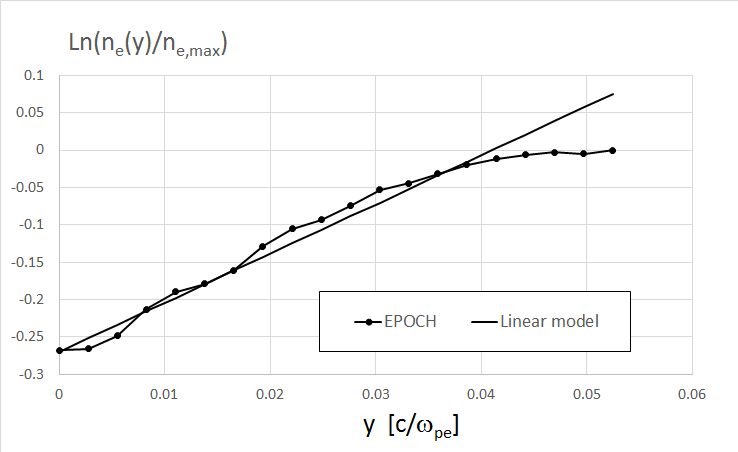
Figure 12: Inhomogeneous particle ionization problem: comparison of the EPOCH solution (solid line with dots) with the y-profile of the electron number density in the linear model, according to Eq.(20).

III Conclusions

In this work we present PIC simulations of free charge creation by collisional ionization of C12 and C60 particles in plasma for the parameters of relevance to plasma gasification. For plasma simulations a fully collisional EPOCH model is used and the obtained solutions are reasonably non-sensitive to the numerical parameters such as the grid resolution, the domain size and the PPC number. There are two regimes considered: with and without excitation of the non-uniform electric field on the boundary. Our main findings are as follows:

(i) In uniform plasmas with smooth walls there appear to be two optimal values of $C60:C12$ fraction for free electron production by collisional ionization (i.e. a most efficient discharge condition creation): one is $10:90$ and the other is $80:20$. The first value is in agreement with the experimental results of LCC Engineering who performed gasification tests with relatively low fullerene concentrations.

(ii) In plasmas with rough walls, modelled by comb-like electric field distribution at the boundary, the case of tangential electric field creates a significant charge localization in C12+ and C60+ species. This leads to the most favorable discharge condition creation for tribo-electrically generated plasma.

(iii) Linear analytical models are presented for modelling the particle collision process. Predictions of the models are in an encouraging agreement with the numerical simulation results.

Figure 13: David Tsiklauri was born in Tbilisi, Georgia, in 1972. He received the M.Sci. degree in theoretical physics from Tbilisi State University, Tbilisi, in 1994, and the Ph.D. degree in physics from the University of Cape Town, Cape Town, South Africa, in 1996. He was a Postdoctoral Fellow with the University of Cape Town, Tbilisi State University, Iowa State University, Ames, IA, USA, and University of Warwick, Coventry, U.K. From 2003 to 2009, he was a Lecturer and a Reader with the University of Salford, Greater Manchester, U.K. In 2009, he joined the Queen Mary University of London, where he is currently a Senior Lecturer. His current research interests include novel particle accelerator concepts, plasma wake-field acceleration, enhanced dissipation of MHD waves in inhomogeneous plasmas, collisionless magnetic reconnection, particle acceleration by dispersive Alfven waves, and radio emission generation mechanisms by accelerated electrons.

Figure 14: Sergey Karabasov is Reader in Computational Modelling in Queen Mary University of London, School of Engineering and Materials Science. Sergey obtained MSc in applied mathematics and physics from Moscow Institute of Physics and Technology in 1995 and PhD in Mathematical Modelling from Moscow Lomonosov State University in 1999. Prior to joining Queen Mary as a Senior Lecturer in 2012, he was a Royal Society University Research Fellow in Cambridge University Engineering Department developing hybrid methods for computational aeroacoustics. In 2010, Sergey was awarded the Full Doctorate of Science (Habilitation Degree) from Keldysh Institute of Applied Mathematics, Moscow for his work on hybrid and direct models in computational aeroacoustics. Sergey’s work typically combines high-resolution computational methods (large-eddy simulations, numerical schemes, high-performance computing) with model decomposition approaches in aero- and hydro-dynamics (acoustic analogy, integral surface methods, vortex sound theory, ocean modelling) and multiscale modelling (bridging continuum mechanics with atomistic simulations).

Figure 15: Vladimir Grigorievich Prodaevich graduated from the Mari Polytechnic Institute in 1980. He worked in forestry in the Nizhny Novgorod region until 1992. In 1992 he was appointed Director General of the Russian Forest Association. He developed a technology for the utilization of waste from the Balakhna PPM with the production of highly effective biologically active substances. From 1994 to 1999, he was the Chairman of the Board of Directors of the Dubitel plant in Vyshny Volochyok. During these years he developed a technology for obtaining new types of products from spruce and willow bark. He developed a preparation for clarification of wine materials and juices as well as a technology for the production of environmentally friendly wood-based panels for housing construction. He is also an author of a preparation for increasing of the strength of the hermetic layer of tubeless car tires. When leading the Central Research Forest Chemical Institute (TsNILHI) he developed a technology for producing bitulin from birch bark. He also developed a technology of complex processing of spruce bark to produce lipids, tannides, pectins in a single technological process. The developments include a continuous retort for the production of charcoal with the utilization of exhaust gases using a plasma gasifier. Since 2009 he has been working on the improvement of the design of a plasma gasifier for various purposes. His recent work on the design of tribo-electric plasma gasifiers has been with Engineering Company Eco-Ardens.