Improved BiGAN training with marginal
likelihood equalization

\namePablo Sánchez-Martín \emailpablo.sanchez-martin@tuebingen.mpg.de
\addrMax Planck Institute for Intelligence Systems
Tübingen, Germany \AND\namePablo M. Olmos \emailolmos@tsc.uc3m.es
\addrUniversity Carlos III in Madrid
Madrid, Spain \AND\nameFernando Perez-Cruz \emailfernando.perezcruz@sdsc.ethz.ch
\addrSwiss Data Science Center (ETH Zürich)
Zürich/ Laussane, Switzerland

Abstract

We propose a novel training procedure for improving the performance of generative adversarial networks (GANs), especially to bidirectional GANs. First, we enforce that the empirical distribution of the inverse inference network matches the prior distribution, which favors the generator network reproducibility on the seen samples. Second, we have found that the marginal log-likelihood of the samples shows a severe overrepresentation of a certain type of samples. To address this issue, we propose to train the bidirectional GAN using a non-uniform sampling for the mini-batch selection, resulting in improved quality and variety in generated samples measured quantitatively and by visual inspection. We illustrate our new procedure with the well-known CIFAR10, Fashion MNIST and CelebA datasets.

1 Introduction

Implicit generative modeling, in general, and Generative Adversarial Networks (GANs) (Goodfellow et al., 2014), in particular, promise to solve the universal simulator problem in an end-to-end fashion (Goodfellow et al., 2014; Kingma and Welling, 2014; Mohamed and Lakshminarayanan, 2016). GANs have been successfully applied to a variety of tasks, such as image-to-image translation (Isola et al., 2017), image super-resolution (Ledig et al., 2017), image in-painting (Pathak et al., 2016), domain adaptation (Kim et al., 2017), text-to-image synthesis (Zhang et al., 2017), dark matter estimation (Rodriguez et al., 2018), and breaking federated learning systems (Hitaj et al., 2017), among many others. Progress in GANs has been quite remarkable and fast in the past four years. Most of the work has concentrated on improving its training to make it more stable, robust and generalizable to numerous architectures and datasets (Nowozin et al., 2016; Gulrajani et al., 2017; Arjovsky et al., 2017; Li et al., 2017; Miyato et al., 2018) to name a few. All these approaches focus on learning the unidirectional mapping from a low-dimensional embedding $\mathbf{z}$ to the high-dimensional data space $\mathbf{x}$ . Several works in the literature have reported that the latent space of GANs drives semantically meaningful representations (Chen et al., 2016). Further, data augmentation and image editing techniques can be built upon the latent space of GANs (Radford et al., 2015; Berthelot et al., 2017; Bau et al., 2019).

Another interesting extension to GANs are ALI (Dumoulin et al., 2017) and BiGAN (Donahue et al., 2017) that propose a novel framework for training bidirectional GANs, that jointly learns the bidirectional mapping between $\mathbf{z}$ and $\mathbf{x}$ in an unsupervised manner. They use the generator similar to unidirectional GANs (Radford et al., 2015; Mao et al., 2017; Gulrajani et al., 2017; Warde-Farley and Bengio, 2017) for constructing the forward mapping from $\mathbf{z}$ to $\mathbf{x}$ , and then use an encoder network to model the inference mapping from $\mathbf{x}$ to $\mathbf{z}$ . The discriminator network is now trained to distinguish the joint distribution of $(G(\mathbf{z}),\mathbf{z})$ from that of $(\mathbf{x},E(\mathbf{x}))$ , where $E(\cdot)$ and $G(\cdot)$ respectively denote the mapping functions defined by the encoder and the generator. Although their models can reconstruct the original image from the estimated latent variable, the visual quality of the generation is generally worse than the unidirectional GANs. MDGAN (Che et al., 2017), unlike ALI and BiGAN, introduces an additional constraint to enforce that the reconstructed images are identical to the original images, namely the reconstruction loss. VEEGAN (Srivastava et al., 2017) also includes a reconstruction loss on the latent space to also improve reconstruction quality.

In this paper, we address several technical challenges not yet reported for (bidirectional) GANs. First, while the reconstructed images $G(E(\mathbf{x}))$ by MDGAN are accurate, we notice that the empirical distribution induced by $E(\mathbf{x})$ at the latent space $\mathbf{z}$ for both train and test images is not from the typical set of the latent space distribution¹¹1This issue also appears in standard BiGAN.. For example, if $p(\mathbf{z})$ is a $D$ -dimensional Gaussian, then the induced $||E(\mathbf{x})||_{2}$ from MDGAN training is typically much larger than $\sqrt{D}$ , thus implying that the real images are not typical from the latent distribution standpoint. To address this issue, we include in the loss function a second regularization term that penalizes $||E(\mathbf{x})||_{2}\neq\sqrt{D}$ .

Second, once the encoder maps the training (and test) images to the typical set of the latent space, we study the marginal log-likelihood per image in both the train and test sets. We noticed that the log-likelihood distribution is extremely asymmetric, this issue was not raised by (Wu et al., 2017), in which the marginal likelihood was first computed for GANs/VAEs. To compensate for this effect, we propose to train MDGAN using two non-uniform sampling schemes. In the first scheme, we use the estimated marginal log-likelihood to reweigh the training samples probability of being added to each mini-batch. In the second approach, the reweighing uses the reconstruction quality as a proxy to measure the marginal log-likelihood. The use of reconstruction quality instead of marginal likelihood was proposed upon observing that both quantities are highly correlated, i.e., overrepresented images are typically reconstructed with higher quality, and computing log-likelihood is computationally expensive, while reconstruction quality can be easily measured after each mini-batch has been trained. We found that this second approach improves both the quality of the generated images, and the diversity of the generative model.

2 Related Work

2.1 BiGAN and MDGAN

Currently, there exist several variants GANs that allow performing inference over the latent variable. One of these models is the Bidirectional Generative Adversarial Network (BiGAN) (Donahue et al., 2017) which includes an inference or encoder network denoted as $E(\mathbf{x})$ that learns a mapping from data points $\mathbf{x}$ into the latent space $\mathbf{z}$ . Now, the discriminator aims at distinguishing between real tuples $(\mathbf{x},E(\mathbf{x}))$ and fake tuples $(G(\mathbf{z}),\mathbf{z})$ , thus it is denoted as $D(\mathbf{x},\mathbf{z})$ . The optimization of the model reads as follows:

\begin{split}\mathcal{L}_{\mathrm{BiGAN}}&:=\mathbb{E}_{\mathbf{x}\sim p_{\mathbf{X}}}\left[\mathbb{E}_{\mathbf{z}\sim p_{E}(\cdot|\mathbf{x})}[\log D(\mathbf{x},\mathbf{z})]\right]+\mathbb{E}_{\mathbf{z}\sim p_{\mathbf{Z}}}\left[\mathbb{E}_{\mathbf{x}\sim p_{G}(\cdot|\mathbf{z})}[\log(1-D(\mathbf{x},\mathbf{z}))]\right]\end{split}

(1)

Donahue et al. (2017) demonstrate that at the global optimum, G and E are each other’s inverse. Unfortunately, in practice we are only able to arrive at a local optimum. As a consequence, the reconstruction of a sample, $G(E(\mathbf{x}))$ , has margin for improvement. Che et al. (2017) propose to add a reconstruction loss term

\displaystyle\mathcal{L}_{\mathrm{cyc}}(G,E)=\mathbb{E}_{\mathbf{x}\sim p_{r}(\mathbf{x})}[d(G(E(\mathbf{x})),\mathbf{x})]

(2)

to the original objective function in order to drive better reconstructions. This term measures the reconstruction error based on some distance metric $d(\cdot,\cdot)$ , typically minimum squared error. They named the resulting model MDGAN. The updated objective function is $\mathcal{L}(D,G,E)=\mathcal{L}_{\mathrm{BiGAN}}+\lambda_{\text{cyc}}\mathcal{L}_{\mathrm{cyc}}(G,E)$ , where $\lambda_{\text{cyc}}$ is a new hyperparameter controlling the reconstruction quality. Results show a clear improvement in the reconstructed data points, as expected.

2.2 Data log-likelihood in GANs

The likelihood of a test sample can be computed as follows:

p(\mathbf{x}_{\text{test}})=\int p(\mathbf{x}_{\text{test}}|\mathbf{z})p(\mathbf{z})d\mathbf{z},

(3)

In Wu et al. (2017), the authors proposed an isotropic Gaussian likelihood for GANs, i.e:

p(\mathbf{x}_{\text{test}}|\mathbf{z})\approx\frac{1}{(2\pi\sigma^{2})^{\dim(\mathbf{x})}}\exp\left(\frac{||\mathbf{x}_{\text{test}}-G(\mathbf{z})||^{2}}{2\sigma^{2}}\right).

(4)

They solved the integral in (3) by annealed importance sampling (Neal, 2001). This model for $p(\mathbf{x}_{\text{test}}|\mathbf{z})$ is a fine choice, if the error in the generated images comes from noisy observations and there is not a significant model misspecification. But when the error in GAN generation comes from model misspecification (i.e. there is little noise in images datasets) finding the appropriate $\sigma$ becomes an impossible task, because not all samples will be equally represented by the model. In this case, there is no right $\sigma$ that helps us evaluate the marginal likelihood accurately for our model. When the reconstruction can be uneven, best reconstructed images would seem more likely, which does not need to be the case. Hence, the estimated likelihood can be biased by the sample’s reconstruction quality in a way that does not allow distinguishing which one is at play.

More recently, Balaji et al. (2019) proposed an approach to compute data log-likelihood for optimal transport GANs, e.g. Wasserstein GAN (Arjovsky et al., 2017), based on three main components: the distance between real samples and the generative model, the entropy of the posterior distribution and the likelihood of the coupled latent variable. They also propose a modification of their approach to be used in a general GAN by not taking into account the entropy term.

3 Prior Regularized MDGAN

While MDGAN is designed to provide realistic reconstruction of the original image $\mathbf{x}\approx G(E(\mathbf{x}))$ , it ignores the fact that latent projections produced by $E(\mathbf{x})$ can be untypical under the latent-space model $p(\mathbf{z})$ , where $p(\mathbf{z})$ is usually taken as an independent high-dimensional Gaussian distribution (or other simple distribution).

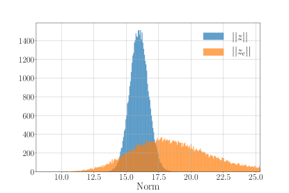
For example, we have trained an MDGAN with a 5-layer generator network, a 7-layer discriminative network and a 256-dimension latent space (see the specific network structural details in Appendix A) with the images from CIFAR10. We have taken the 45,000 training images and we have recovered the latent space representation $\mathbf{z}_{i}=E(\mathbf{x}_{i})$ . In Figure 1 (a), we plot the histogram of the norm of these latent space representation (in orange). For comparison, we plot the histogram of the norm of 45,000 samples from $p(\mathbf{z})$ in blue. Observe that there is an important fraction of images for which $||\mathbf{z}_{i}||$ is outside the typical set of $p(\mathbf{z})$ and they will not be generated when sampling from $p(\mathbf{z})$ , since the prior probability mass decays exponentially fast with $||\mathbf{z}||^{2}$ . To address this issue, we propose to add a simple additional regularizer to the MDGAN objective function:

\displaystyle\mathcal{L}_{\mathrm{norm}}(E)=\mathbb{E}_{\mathbf{x}\sim p_{r}(\mathbf{x})}\left[\left(||E(\mathbf{x})||_{2}-\sqrt{\text{dim}(\mathbf{z})}\right)^{2}\right],

(5)

which penalizes values of the norm of $E(\mathbf{x})$ that lay outside the typical set. For other prior distributions, this regularizer should be adjusted accordingly. Finally, the objective function of this new scheme, we refer to as Prior-regularized MDGAN (P-MDGAN), is:

\displaystyle\mathcal{L}(D,G,E)=\mathcal{L}_{\mathrm{BiGAN}}+\lambda_{\text{cyc}}\mathcal{L}_{\mathrm{cyc}}+\lambda_{\text{norm}}\mathcal{L}_{\mathrm{norm}},

(6)

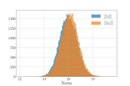
where $\lambda_{\text{norm}}$ is an automatically-tuned hyperparameter during training that ensures the distribution of the encoded latent vectors matches the prior distribution (details can be found in Appendix B). In the Figure 1 (b), we show the norm of the latent space representation of the same 45,000 training images used for MDGAN, in which we can see that the P-MDGAN latent space ensures the samples are mapped to the typical set.

4 Equalized MDGAN training

In this section, we describe our second contribution of this paper. We first note that the marginal likelihood and reconstruction quality between the original images and the reconstructed images varies orders of magnitude and we propose to adapt the training of GANs to try to equalize both. In Section 2, we presented two methods to compute the marginal likelihood that mixed in a single number both the marginal likelihood and reconstruction quality. In this paper, we also advocate for measuring both of them independently, because we believe that each one of them provide us with different information that would be useful to improve the performance of bi-directional GANs. In this paper, we also go one step further and propose to use these measurements to modify the training and as consequence improve the performance of the resulting GAN.

Instead of estimating the marginal likelihood in (3), we propose to compute the marginal likelihood of the reconstructed image, i.e.:

p(G(E(\mathbf{x})))=\int p(G(E(\mathbf{x}))|\mathbf{z})p(\mathbf{z})d\mathbf{z},

(7)

because in this way we know how likely it is the generated image from a given $\mathbf{z}$ , independent of the reconstruction quality. We also measure the quality of the reconstructed image using the mean squared error, as proposed in the original MDGAN paper to enforce reconstruction quality (Che et al., 2017). We actually report the Peak Signal-to-Noise Ratio (PSNR):

\displaystyle\text{PSNR}(\mathbf{x},G(E(\mathbf{x})))=10\log_{10}\left(\frac{3\times K\times M^{2}}{||\mathbf{x}-G(E(\mathbf{x}))||^{2}}\right),

where 3 is the number of color channels, $K$ is the number of pixels in the image and $M$ is the maximum possible pixel value of the images, i.e. 255 for 8-bit color images.

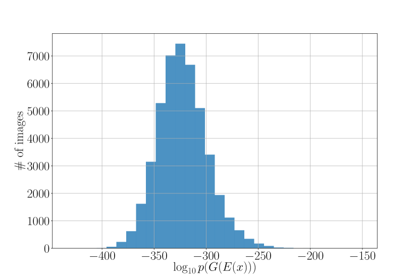
For illustration purposes, we consider a P-MDGAN trained over CIFAR10, as in the previous section. In Figure 3, we report the log-likelihood of the 45,000 reconstructed training images computed using a similar procedure to Wu et al. (2017) for (7). Considering that every image was used equally during training, we would expect that they all have similar log-likelihoods, yet we observe the differences are quite significant. The values shown are in $\log_{10}$ , this means the differences are in the order of $10^{100}$ between the most generated images and the least generated images.

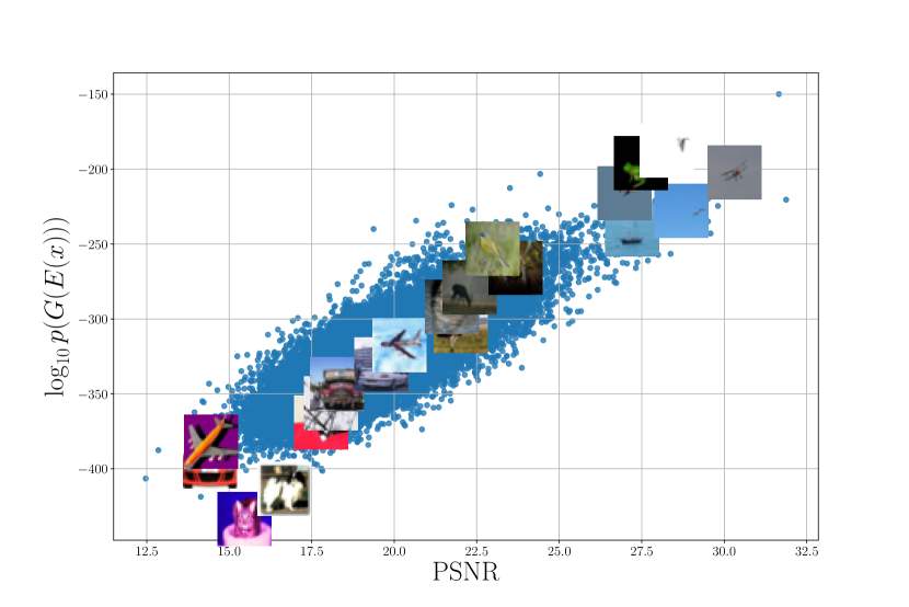
These results indicate that the P-MDGAN is substantially over-representing a small subset of images, which are orders of magnitude more likely than the rest of the images. Figure 3 shows a scatter plot comparing the reconstruction quality of $G(E(\mathbf{x}))$ w.r.t. the original image $\mathbf{x}$ measured in PSNR versus their corresponding estimated marginal log-likelihood, we can observe that images with simpler textures and large uniform backgrounds are not only reconstructed with better quality but also they are being overrepresented by the generator network. In parallel to our work, (Krusinga et al., 2019) also acknowledged this phenomenon.

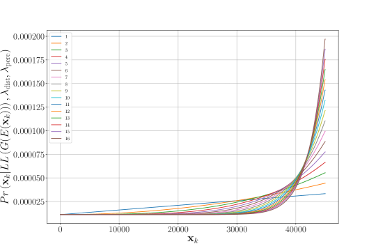
In order to improve the diversity and reconstruction quality of the generated/reconstructed images, we propose to retrain the P-MDGAN from scratch using non-uniform sampling. We rely on the marginal log-likelihood estimation from the first P-MDGAN to boost the marginal likelihood and reconstruction quality of the less represented samples. The main idea is to resample more frequently in the mini-batches those samples with lowest marginal likelihood. We use a simple scheme that shows significant improvements²²2This is a first attempt to show that non-uniform sampling is useful to train GANs, further research is needed to find an optimal resampling strategy., In particular, we first sort the images according to their $LL(G(E(\mathbf{x}_{k})))=\log_{10}p(G(E(\mathbf{x}_{k})))$ from larger to smaller, their probability in the non-uniform distribution will be proportional to the position $k\in[1,2,\ldots,N]$ they hold in the sorted list, raised to the power of $\lambda_{\text{dist}}\geq 0$ . Additionally, we introduce a second hyperparameter, $\lambda_{\text{perc}}\in[0,1]$ , to control the percentage of samples per mini-batch that use this re-weighting strategy, while the remaining are chosen uniformly. We refer to this non-uniform sampling scheme as P-MDGAN with MLeq, where MLeq stands for Marginal Likelihood equalization training. The probability of a sample being added to each mini-batch is given by:

\displaystyle Pr(\mathbf{x}_{k}|LL(G(E(\mathbf{x}_{k}))),\lambda_{\text{dist}},\lambda_{\text{perc}})=\frac{1-\lambda_{\text{perc}}}{N}+\lambda_{\text{perc}}\frac{\left(k/100\right)^{\lambda_{\text{dist}}}}{\sum_{j=1}^{N}\left(j/100\right)^{\lambda_{\text{dist}}}}.

Figure 4 shows the resulting distribution for different values of $\lambda_{\text{dist}}$ .

Our experimental results show that this resampling strategy improves the sample diversity of the generative model (see Section 5). Nonetheless, this training procedure is computational expensive considering we must compute the marginal log-likelihood for all the training images and perform a second round of training. Since we have observed that there exists an almost linear relation between the marginal log-likelihood and the PSNR (See Figure 3), we propose to use the PSNR as a proxy for the marginal log-likelihood to decide the reweighing of the samples into each one of the mini-batches. Computing the PSNR is quite inexpensive, and we can hence recompute the PSNR for each image after each mini-batch has been trained and use the new PSNR to decide which samples should be added to the next mini-batch. We use the same weighting function as in (B), replacing $LL(G(E(\mathbf{x}_{k})))$ by $\text{PSNR}(\mathbf{x}_{k},G(E(\mathbf{x}_{k})))$ and sorting the samples according to their PSNR. In this way, we do not need to do the training procedure twice, but just have a single procedure that ensures diversity and quality are improved in every step. We refer to this procedure as Equalized Prior-regularized MDGAN, or EP-MDGAN, which incorporates the prior regularization from the previous section to make sure all the samples are matched to the typical set and the PSNR equalization to improve sample diversity and reconstruction quality.

5 Experiments

5.1 Experimental Setup

We have conducted a broad set of experiments in order to empirically demonstrate the validity of the regularization techniques proposed. Here, we present the results obtained with the models trained over the CIFAR10, F-MNIST and CelebA datasets with the configuration of hyperparameters that yield to the best FID scores, shown in Table 1. We split the CIFAR10 dataset in 45,000 training, 5,000 validation, and 1,0000 test examples; the F-MNIST contains 54,000 training, 6,000 validation, and 1,0000 test examples; and the CelebA contains 180,540 training, 20,060 validation, and 1,999 test examples. Appendix B contains further details about the hyperparameter cross-validated and Appendix C contains further results.

	$\lambda_{\text{cyc}}$	$\lambda_{\text{perc}}$	$\lambda_{\text{dist}}$
MDGAN	8 (9)	-	-
P-MDGAN	7 (9)	-	-
P-MDGAN with ML	5 (5)	0.5 (0.8)	8 (8)
EP-MDGAN	3 (3)	0.5 (0.8)	12 (4)

Table 1: Configuration of hyperparameters for CIFAR10 and F-MNIST. F-MNIST are denoted in parenthesis.

Metrics:

We measure the FID score, which is considered the state-of-the-art measure for GANs. It provides us a way to identify poor performance but being a single scalar metric is unable to distinguish between sample quality and distribution coverage. We also rely on Kynkäänniemi et al. (2019) to distinguish between both type of failures. Kynkäänniemi et al. (2019) proposes a 2-dimensional metric based on the notion of precision and recall that matches our understanding of sample quality and distribution coverage. We also inspect the quality of the reconstructed images measured in PSNR, described in Section 4. Finally, we visually show how our method improves variety in the generated samples.

Experimental setup:

We use the MDGAN as the baseline and compared it with the models we proposed: P-MDGAN and P-MDGAN with the two non-uniform sampling schemes, namely P-MDGAN with MLeq and EP-MDGAN. We only computed P-MDGAN with MLeq for the CIFAR10 dataset because it is computationally expensive and EP-MDGAN achieves similar performance. We trained all the models for 800 epochs using the Adam optimizer (Kingma and Ba, 2015), stochastic gradient descent with a batch size of 128 and we use spectral normalization GANs (Miyato et al., 2018). Additionally, we cross-validated the regularization parameters $\lambda_{\text{cyc}}$ , $\lambda_{\text{dist}}$ , $\lambda_{\text{perc}}$ to have a complete understanding of their effect on the outcome. For all the models, we defined their three elements, namely $G(\cdot)$ , $D(\cdot)$ and $E(\cdot)$ , as convolutional neural networks with 5, 10 and 7 layers respectively. We consider a Gaussian noise model for the latent variable $\mathbf{z}\sim\mathcal{N}(\mathbf{0},\mathbf{I})$ with $\text{dim}(\mathbf{z})=256$ .

To facilitate reproducibility of our results, in Appendix A and Appendix B we provide an exhaustive description of the networks architecture and parameters selected regarding the training process. PyTorch implementation for the models is available at https://github.com/psanch21/imp_bigan.

5.2 Generated samples

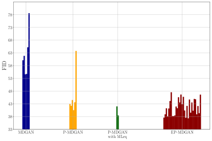
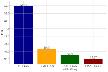
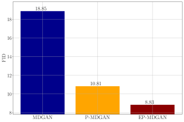
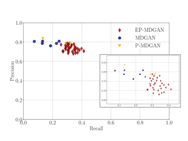
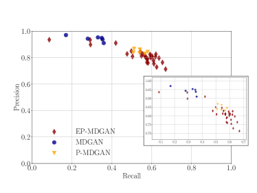
Figure 5 shows the FID values computed over test samples of the CIFAR10 and F-MNIST datasets. If we focus on Figure 5 (a), we can observe that the worst FID scores are obtained for MDGAN and P-MDGAN, and that the FID decreases (improves) when using any of the non-uniform sampling schemes, obtaining the best FID score for EP-MDGAN. Although these are the results for a specific configuration of the hyperpameters we have found that for most of the configurations these results hold. To gain more insights about the reason of this improvement, Figure 6 shows a scatter plot of the Precision vs Recall scores obtained for all trained models. Observe the different EP-MDGAN models trained suffer a small precision drop and improved recall by over two-fold. This is an indication that the non-uniform sampling procedure encourages diversity in generated samples. The non-uniform sampling also provides a way to trade-off precision and recall in bi-directional GANs that can provide better diversity at the expense of limited image quality degradation.

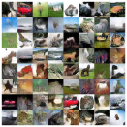
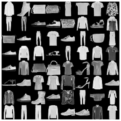
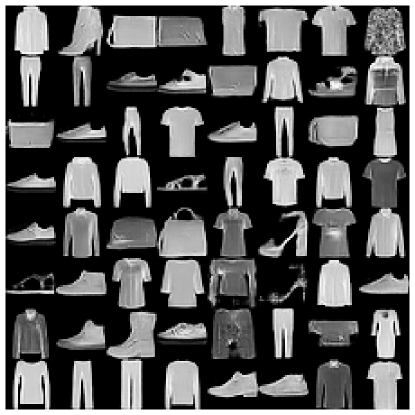
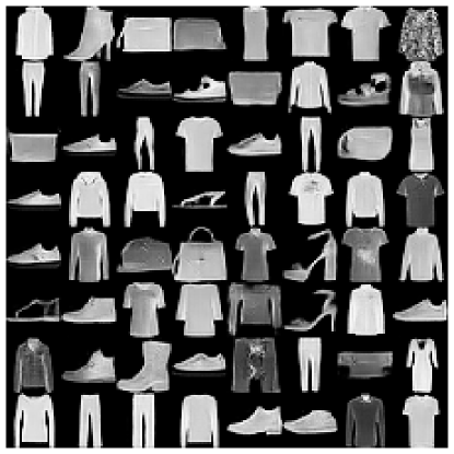
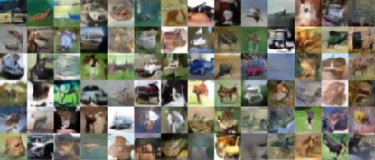
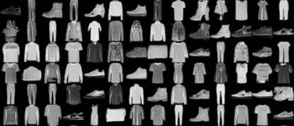
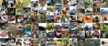
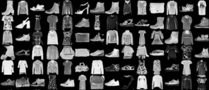
We can also evaluate this improvement by visually inspecting generated samples, shown in Figure 7 which shows samples generated for the CIFAR10 (left column) and F-MNIST (right column) datasets using the MDGAN (top row) and EP-MDGAN (bottom row). If we focus our attention to the left column, we observe samples generated using MDGAN, namely Figure 7 (a), contain homogeneous backgrounds and simple objects with a spectrum of colors mainly limited to green, brown and blue tones. On the contrary, images produced by EP-MDGAN include diversity of color, and more complex backgrounds and shapes. This behavior is also acknowledged in the generated F-MNIST samples from EP-MDGAN, the images contain irregular patterns, textures, and more high heels. We also include in Figure 8 samples generated for the CelebA dataset. We can observe the EP-MDGAN generates faces with glasses (bordered in green) or other accessories, which similarly as with previous datasets can be considered as complex examples.

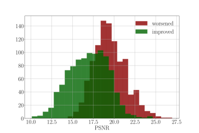
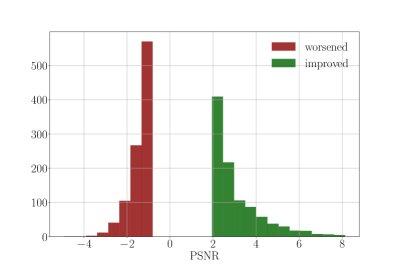
Reconstruction quality: Figure 9 (a) shows two histograms of the PSNR computed between CIFAR10 test images and their corresponding MDGAN reconstruction. The histogram in green represents the $10\%$ of images that improve the reconstruction PSNR using EP-MDGAN the most. Similarly, the red histogram represents the $10\%$ of images that worsen the most the reconstruction PSNR using EP-MDGAN.

These results shows that the non-uniform sampling training encourages better reconstruction of the images that obtained worse reconstruction quality, i.e. visually complex examples, when using the baseline. As such, a slight decrease of reconstruction quality in the subset of simpler images does not bring a noticeable visual impact. Figure 9 (b) shows the order or improvement/deterioration.

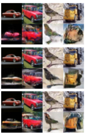
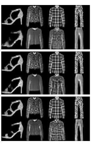
In Figure 10 we show 4 visually complex images from the CIFAR10 and F-MNIST test sets and their corresponding reconstructions. We observe that P-MDGAN and EP-MDGAN achieve better qualitative reconstruction quality than MDGAN.

6 Conclusion

In this paper we have first proposed a novel regularization on the inference network of the BiGAN so that the distribution of the encoded latent space variables matches the prior distribution. This means that the latent representation of samples lays in the typical set and the corresponding reconstruction is likely to be sampled from the generative model. We called the resulting model P-MDGAN.

Then we introduce a method to estimate marginal log-likelihood over reconstructed images, rather than original samples. We provide an explanation of why log-likelihood and reconstruction quality should be computed independently so that the latter does not bias the first. The reproduction quality tells us if a sample can be generated by the GAN and how good it matches the test sample³³3This measure had been proposed previously in Zhu et al. (2016); Metz et al. (2017), but has not been advocated for systematically evaluating GANs.. The estimation of the log-likelihood of the reconstruction tells us how likely are we to see that reconstruction, which is the only image that the GAN can produce. Estimating the likelihood of the test sample directly is much harder and it mixes these two relevant metrics in one, making it useless to evaluate GANs, as already point it out in Theis et al. (2016).

The results in log-likelihood estimation show that training and test samples suffer significant over and under-representation issues that need to be corrected when training GANs. We have also noticed that the samples that are more visually complex lead to higher reconstruction error and lower marginal likelihoods. For example, we can argue that the samples that present lower marginal likelihood can be over-sampled when training GANs, as we should not expect that harder to generate samples need to be seen an equal number of times that those that are easier to generate. We finally proposed to train the GANs using a non-uniform sampling scheme and we propose two approaches for that, one of them static (for computational reasons) based on the estimated log-likelihoods, and the other one dynamical using the PSNR between original images and reconstructions. We show they improve the baseline in terms of image diversity while also improving the reconstruction of visually complex images.

Acknowledgments

The work of Pablo M. Olmos is supported by Spanish government MCI under grant PID2019-108539RB-C22 and RTI2018-099655-B-100, by Comunidad de Madrid under grants IND2017/TIC-7618, IND2018/TIC-9649, and Y2018/TCS-4705, by BBVA Foundation under the Deep-DARWiN project, and by the European Union (FEDER and the European Research Council (ERC) through the European Unions Horizon 2020 research and innovation program under Grant 714161). We also gratefully acknowledge the support of NVIDIA Corporation with the donation of the Titan X Pascal GPU used for this research.

References

Arjovsky et al. (2017) Martin Arjovsky, Soumith Chintala, and Léon Bottou. Wasserstein Generative Adversarial Networks. In Proceedings of the 34th International Conference on Machine Learning, 2017.
Balaji et al. (2019) Yogesh Balaji, Hamed Hassani, Rama Chellappa, and Soheil Feizi. Entropic GANs meet VAEs: A Statistical Approach to Compute Sample Likelihoods in GANs. In International Conference on Machine Learning, 2019.
Bau et al. (2019) David Bau, Hendrik Strobelt, William Peebles, Jonas Wulff, Bolei Zhou, Jun-Yan Zhu, and Antonio Torralba. Semantic photo manipulation with a generative image prior. ACM Transactions on Graphics (TOG), 2019.
Berthelot et al. (2017) David Berthelot, Thomas Schumm, and Luke Metz. Began: Boundary equilibrium generative adversarial networks. arXiv preprint arXiv:1703.10717, 2017.
Che et al. (2017) Tong Che, Yanran Li, Athul Paul Jacob, Yoshua Bengio, and Wenjie Li. Mode regularized generative adversarial networks. International Conference on Learning Representations (ICLR), 2017.
Chen et al. (2016) Xi Chen, Yan Duan, Rein Houthooft, John Schulman, Ilya Sutskever, and Pieter Abbeel. Infogan: Interpretable representation learning by information maximizing generative adversarial nets. In Advances in Neural Information Processing Systems, 2016.
Donahue et al. (2017) Jeff Donahue, Philipp Krähenbühl, and Trevor Darrell. Adversarial feature learning. International Conference on Learning Representations (ICLR), 2017.
Dumoulin et al. (2017) Vincent Dumoulin, Ishmael Belghazi, Ben Poole, Olivier Mastropietro, Alex Lamb, Martin Arjovsky, and Aaron Courville. Adversarially learned inference. International Conference on Learning Representations (ICLR), 2017.
Goodfellow et al. (2014) Ian Goodfellow, Jean Pouget-Abadie, Mehdi Mirza, Bing Xu, David Warde-Farley, Sherjil Ozair, Aaron Courville, and Yoshua Bengio. Generative Adversarial Nets. In Advances in neural information processing systems, pages 2672–2680, 2014.
Gulrajani et al. (2017) Ishaan Gulrajani, Faruk Ahmed, Martin Arjovsky, Vincent Dumoulin, and Aaron C Courville. Improved Training of Wasserstein GANs. In Advances in Neural Information Processing Systems. 2017.
Hitaj et al. (2017) Briland Hitaj, Giuseppe Ateniese, and Fernando Perez-Cruz. Deep models under the GAN: information leakage from collaborative deep learning. In Proceedings of the 2017 ACM SIGSAC Conference on Computer and Communications Security, 2017.
Isola et al. (2017) Phillip Isola, Jun-Yan Zhu, Tinghui Zhou, and Alexei A. Efros. Image-to-Image Translation with Conditional Adversarial Networks. IEEE Conference on Computer Vision and Pattern Recognition (CVPR), 2017.
Kim et al. (2017) Taeksoo Kim, Moonsu Cha, Hyunsoo Kim, Jung Kwon Lee, and Jiwon Kim. Learning to Discover Cross-Domain Relations with Generative Adversarial Networks. In Proceedings of the 34th International Conference on Machine Learning, 2017.
Kingma and Ba (2015) Diederik P Kingma and Jimmy Ba. Adam: A method for stochastic optimization. International Conference on Learning Representations (ICLR), 2015.
Kingma and Welling (2014) Diederik P Kingma and Max Welling. Auto-encoding variational bayes. In International Conference on Learning Representations (ICLR), 2014.
Krusinga et al. (2019) Ryen Krusinga, Sohil Shah, Matthias Zwicker, Tom Goldstein, and David Jacobs. Understanding the (un) interpretability of natural image distributions using generative models. arXiv preprint arXiv:1901.01499, 2019.
Kynkäänniemi et al. (2019) Tuomas Kynkäänniemi, Tero Karras, Samuli Laine, Jaakko Lehtinen, and Timo Aila. Improved precision and recall metric for assessing generative models. In Advances in Neural Information Processing Systems, 2019.
Ledig et al. (2017) Christian Ledig, Lucas Theis, Ferenc Huszar, Jose Caballero, Andrew Cunningham, Alejandro Acosta, Andrew Aitken, Alykhan Tejani, Johannes Totz, Zehan Wang, and Wenzhe Shi. Photo-Realistic Single Image Super-Resolution Using a Generative Adversarial Network. In IEEE Conference on Computer Vision and Pattern Recognition (CVPR), 2017.
Li et al. (2017) Chun-Liang Li, Wei-Cheng Chang, Yu Cheng, Yiming Yang, and Barnabás Póczos. MMD GAN: Towards deeper understanding of moment matching network. In Advances in Neural Information Processing Systems, 2017.
Mao et al. (2017) Xudong Mao, Qing Li, Haoran Xie, Raymond YK Lau, Zhen Wang, and Stephen Paul Smolley. Least squares generative adversarial networks. In The IEEE International Conference on Computer Vision (ICCV), 2017.
Metz et al. (2017) Luke Metz, Ben Poole, David Pfau, and Jascha Sohl-Dickstein. Unrolled Generative Adversarial Networks. In International Conference on Learning Representations (ICLR), 2017.
Miyato et al. (2018) Takeru Miyato, Toshiki Kataoka, Masanori Koyama, and Yuichi Yoshida. Spectral normalization for Generative Adversarial Networks. International Conference on Learning Representations (ICLR), 2018.
Mohamed and Lakshminarayanan (2016) Shakir Mohamed and Balaji Lakshminarayanan. Learning in Implicit Generative Models. arXiv preprint arXiv:1610.03483, 2016.
Neal (2001) Radford M Neal. Annealed importance sampling. Statistics and computing, 2001.
Nowozin et al. (2016) Sebastian Nowozin, Botond Cseke, and Ryota Tomioka. f-GAN: Training Generative Neural Samplers using Variational Divergence Minimization. In Advances in Neural Information Processing Systems. 2016.
Pathak et al. (2016) Deepak Pathak, Philipp Krahenbuhl, Jeff Donahue, Trevor Darrell, and Alexei A. Efros. Context Encoders: Feature Learning by Inpainting. In The IEEE Conference on Computer Vision and Pattern Recognition (CVPR), 2016.
Radford et al. (2015) Alec Radford, Luke Metz, and Soumith Chintala. Unsupervised representation learning with deep convolutional generative adversarial networks. arXiv preprint arXiv:1511.06434, 2015.
Rodriguez et al. (2018) Andres C Rodriguez, Tomasz Kacprzak, Aurelien Lucchi, Adam Amara, Raphael Sgier, Janis Fluri, Thomas Hofmann, and Alexandre Réfrégier. Fast Cosmic Web Simulations with Generative Adversarial Networks. arXiv preprint arXiv:1801.09070, 2018.
Srivastava et al. (2017) Akash Srivastava, Lazar Valkov, Chris Russell, Michael U. Gutmann, and Charles Sutton. Veegan: Reducing mode collapse in gans using implicit variational learning. In Advances in Neural Information Processing Systems. 2017.
Theis et al. (2016) Lucas Theis, Aäron van den Oord, and Matthias Bethge. A note on the evaluation of generative models. International Conference on Learning Representations (ICLR), 2016.
Warde-Farley and Bengio (2017) David Warde-Farley and Yoshua Bengio. Improving generative adversarial networks with denoising feature matching. International Conference on Learning Representations (ICLR), 2017.
Wu et al. (2017) Yuhuai Wu, Yuri Burda, Ruslan Salakhutdinov, and Roger Grosse. On the Quantitative analysis of Decoder-Based Generative Models. International Conference on Learning Representations (ICLR), 2017.
Zhang et al. (2017) Han Zhang, Tao Xu, Hongsheng Li, Shaoting Zhang, Xiaogang Wang, Xiaolei Huang, and Dimitris N. Metaxas. StackGAN: Text to Photo-Realistic Image Synthesis With Stacked Generative Adversarial Networks. In The IEEE International Conference on Computer Vision (ICCV), 2017.
Zhu et al. (2016) Jun-Yan Zhu, Philipp Krähenbühl, Eli Shechtman, and Alexei A. Efros. Generative Visual Manipulation on the Natural Image Manifold. In Proceedings of European Conference on Computer Vision (ECCV), 2016.

A Experiment details

In this section we provide further information about the arquitecture of the networks and training specifications used in our experiments.

Architecture of GANs

The three main blocks, $G(\cdot)$ , $D(\cdot)$ and $E(\cdot)$ , are convolutional neural networks. Considering the networks for a 32x32 image as the reference, the networks for a 28x28 image only change in the second layer of the generator and the networks for a 64x64 image only differ in one layer each. The complete details are in Tables 2, 3 and 4. Following the same approach proposed in the original BiGAN paper, $D(\mathbf{z},\mathbf{x})$ takes $\mathbf{x}$ as input, after some convolutional layers $\mathbf{z}$ is concatenated, and the resulted matrix is passed through several convolutional layers. We use LeakyReLU as activation function with a slope of 0.1 and Spectral normalization. The generator is a 5 layer deconvolutional layer with batch normalization and ReLU as activation function. The inference network $E(\mathbf{x})$ is a 7 layer convolutional network with Leaky ReLU as activation function, followed by a dense layer.

$\mathbf{z}\in\mathbb{R}^{256\times 1\times 1}\sim N(\boldmath{0},\boldmath{I})$
deconv, stride=1, pad=0, $4$ , 512, BN, ReLU
deconv, stride=2, pad=1, $4$ [ $3$ ] , 256, BN, ReLU
deconv, stride=2, pad=1, $4$ , 128, BN, ReLU
deconv, stride=2, pad=1, $4$ , 64, BN, ReLU
deconv, stride=1 (2) , pad=1, $3$ ( $4$ ), 3, Tanh

Table 2: Generator 32 (64)[28]

$\mathbf{x}\in\mathbb{R}^{3\times H\times W}$
conv, stride=1, pad=1, $3$ , 64, SN, LReLU(0.1)
conv, stride=2, pad=1, $4$ , 64, SN, LReLU(0.1)
conv, stride=1 (2), pad=1, $4$ , 128, SN, LReLU(0.1)
conv, stride=2, pad=1, $4$ , 128, SN, LReLU(0.1)
conv, stride=1, pad=0, $4$ , 256, SN, LReLU(0.1)
conv, stride=2, pad=0, $4$ , 256, SN, LReLU(0.1)
$\mathbf{z}\in\mathbb{R}^{256\times 1\times 1}\sim N(\boldmath{0},\boldmath{I})$
conv, stride=1, pad=0, $1$ , 256, SN, LReLU(0.1)
conv, stride=1, pad=0, $1$ , 512, SN, LReLU(0.1)
conv, stride=1, pad=0, $1$ , 1024, SN, LReLU(0.1)
dense, $1024\times 1$

Table 3: Discriminator 32 (64)

$\mathbf{x}\in\mathbb{R}^{3\times H\times W}$
conv, stride=1, pad=1, $3$ , 64, LReLU(0.1)
conv, stride=2, pad=1, $4$ , 64, LReLU(0.1)
conv, stride=1, pad=1, $3$ , 128, LReLU(0.1)
conv, stride=2, pad=1, $4$ , 128, LReLU(0.1)
conv, stride=1 (2), pad=1, $3$ , 256, LReLU(0.1)
conv, stride=2 , pad=1, $4$ , 256, LReLU(0.1)
conv, stride=1 , pad=1, $3$ , 512, LReLU(0.1)
dense, $44512\times 256$

Table 4: Inference 32 (64)

B Training details

The objective function for the PR-BiGAN is

\begin{split}\mathcal{L}(D,G,E)&=\mathcal{L}_{\mathrm{BiGAN}}+\lambda_{\text{cyc}}\mathbb{E}_{\mathbf{x}\sim p_{r}(\mathbf{x})}[d(G(E(\mathbf{x})),\mathbf{x})]\\ &+\lambda_{\text{norm}}\mathbb{E}_{\mathbf{x}\sim p_{r}(\mathbf{x})}\left[\left(||E(\mathbf{x})||_{2}-\sqrt{\text{dim}(\mathbf{z})}\right)^{2}\right]\end{split}

(8)

where the MSE is used as the distance metric in the reconstruction loss. If we set $\lambda_{\text{norm}}=0$ we obtain the MDGANand if we set $\lambda_{\text{cyc}}=0$ the resulting model is the BiGAN. Additionally, we add $\lambda_{\text{perc}}$ and $\lambda_{\text{dist}}$ to perform non-uniform sampling. Basically, these hyperparameters control the different regularization techniques. The parameter $\lambda_{\text{cyc}}\in\mathbb{R}_{\geq 0}$ controls the reconstruction loss; $\lambda_{\text{norm}}\in\mathbb{R}_{\geq 0}$ adapts the regularization on the norm of the distribution induced on the encoder $||E(\mathbf{x})||$ so that it matches the prior distribution; the parameter $\lambda_{\text{perc}}\in[0,1]$ fixes the percentage of uniform samples used in each batch during training; and $\lambda_{\text{dist}}\geq 0$ determines the distribution from which to draw non-uniform samples. This distribution has been computed using the estimated log-likelihoods $LL(\mathbf{x}_{i})$ for a given data set. Firstly we order the images from largest loglikelihood to smaller, $LL(\mathbf{x}_{1})>...>LL(\mathbf{x}_{k})>....>LL(\mathbf{x}_{N})$ , and we keep the location in this list $k$ . Then we use this index $k$ to compute their probability of being sampled: $\lambda_{\text{dist}}\geq 0$ . Additionally, we introduce a second hyperparameter, $\lambda_{\text{perc}}\in[0,1]$ , to control the percentage of samples per mini-batch that use this re-weighting strategy, while the remaining are chosen uniformly.

\displaystyle Pr(\mathbf{x}_{k}|LL(G(E(\mathbf{x}_{k}))),\lambda_{\text{dist}},\lambda_{\text{perc}})=\frac{1-\lambda_{\text{perc}}}{N}+\lambda_{\text{perc}}\frac{\left(k/100\right)^{\lambda_{\text{dist}}}}{\sum_{j=1}^{N}\left(j/100\right)^{\lambda_{\text{dist}}}}.

We have explored different configurations of the regularization hyperparameters $\lambda_{\text{cyc}}$ , $\lambda_{\text{perc}}$ , $\lambda_{\text{dist}}$ in order to demonstrate its performance. They are summarized in Table 5. The regularization paramter $\lambda_{\text{norm}}$ is automatically learnt during training in order to motivate the distribution obtained from $E(\mathbf{x})$ matchs the noise distribution $p(\mathbf{z})=N(\mathbf{z}|\boldmath{0},\boldmath{I})$ . It is initialize with a small value $\lambda_{\text{norm}}=0.01$ which is kept constant for the first 200 epochs and then it is updated according to the variance of $||E(\mathbf{x})||$ computer over all the examples from the train set compared to the variance of $||\mathbf{z}||$ . For all the experiments, we fix the learning rate $2e^{-4}$ , the batch size 128, $\dim(\mathbf{z})=256$ . We train the models for 800 epochs.

		$\lambda_{\text{dist}}$
$\lambda_{\text{cyc}}$	$\lambda_{\text{perc}}$	4	8	12	16
	0.2	✓			✓
3	0.5			✓
	0.8	✓		✓
	0.2	✓	✓
5	0.5		✓	✓
	0.8				✓
	0.2			✓	✓
6	0.5	✓
	0.8			✓	✓
	0.2				✓
7	0.5			✓	✓
	0.8			✓	✓
	0.2		✓
8	0.5	✓		✓
	0.8			✓	✓
	0.2		✓	✓
9	0.5			✓
	0.8		✓		✓

(a) Cifar10

		$\lambda_{\text{dist}}$
$\lambda_{\text{cyc}}$	$\lambda_{\text{perc}}$	4	8	12	16
	0.2				✓
3	0.5	✓	✓
	0.8	✓	✓
	0.2			✓
5	0.5			✓	✓
	0.8			✓	✓
	0.2		✓	✓	✓
6	0.5
	0.8			✓	✓
	0.2				✓
7	0.5		✓	✓
	0.8	✓	✓
	0.2
8	0.5	✓	✓		✓
	0.8			✓	✓
	0.2				✓
9	0.5		✓	✓	✓
	0.8			✓

(b) F-MNIST

		$\lambda_{\text{dist}}$
$\lambda_{\text{cyc}}$	$\lambda_{\text{perc}}$	4	8	12	16
	0.2		✓		✓
3	0.5	✓			✓
	0.8	✓
	0.2		✓		✓
5	0.5				✓
	0.8		✓		✓
	0.2		✓		✓
7	0.5			✓
	0.8	✓	✓

Table 5: Set of hyperparameters validated

We use Adam optimizer with parameters $\beta_{1}=0.5$ and $\beta_{2}=0.999$ and Exponential Learning rate decay 0.99 starting at epoch 400. We alternate between the optimization of the $D(\cdot)$ parameters and the optimization of the $E(\cdot)$ and $G(\cdot)$ parameters jointly. We perform 5 updates of $D(\cdot)$ per 1 update of $G(\cdot)$ and $E(\cdot)$ .

C Additional Results

In this section we extend the results presented in the main paper. For all the models trained with the CIFAR10 dataset, we show the FID scores obtained using the test set in Figure 11 (a) and the train set in Figure 11 (b). Observe that all the configurations of EP-MDGAN trained obtain low and similar FID values while MDGAN and P-MDGAN suffer from high variance, the choice of the $\lambda_{\text{cyc}}$ affects the FID scores.

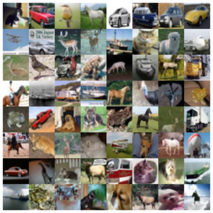
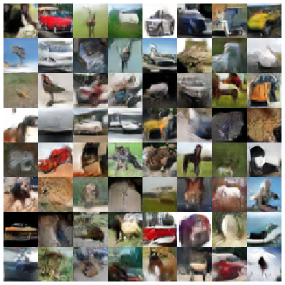
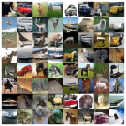
In Figure 12 we show samples from the CIFAR10 traning set and the corresponding reconstructions obtained using the hyperparameter configurations that achieve the best FID scores of MDGAN, P-MDGAN and EP-MDGAN, as performed in the main paper. By visual inspection is it difficult to assess which one ccomplish better reconstruction quality. Nonetheless, the value of $\lambda_{\text{cyc}}$ for EP-MDGAN is considerably smaller than for P-MDGAN or MDGAN which indicates the reweighting schemes requires less regularization to achieve same performance. This behavior also happens for the F-MNIST as shown in Figure 13.

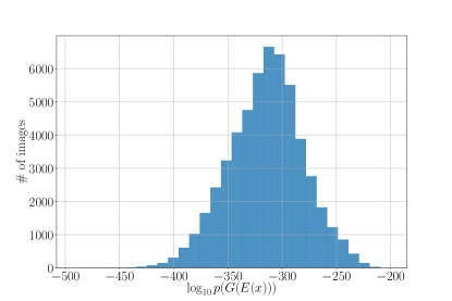
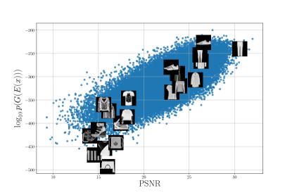
Figure 14 (a) shows the histogram of the marginal log-likelihood of $G(E(\mathbf{x}))$ for all samples in the F-MNIST training set and we can observe the differences are huge, in the order of $10^{100}$ . In Figure 14 (b) we present a scatter plot of the reconstruction quality measured in PSNR versus the marginal likelihood. Similarly as with the CIFAR10 dataset, we observe there is a linear relationship between both variables and that simple plain images obtain are more likely and better reconstructed.