Rigidly rotating gravitationally bound systems
of point particles, compared to polytropes

Abstract

In order to simulate rigidly rotating polytropes we have simulated systems of $N$ point particles, with $N$ up to 1800. Two particles at a distance $r$ interact by an attractive potential $-1/r$ and a repulsive potential $1/r^{2}$. The repulsion simulates the pressure in a polytropic gas of polytropic index $3/2$. We take the total angular momentum $L$ to be conserved, but not the total energy $E$. The particles are stationary in the rotating coordinate system. The rotational energy is $L^{2}/(2I)$ where $I$ is the moment of inertia. Configurations where the energy $E$ has a local minimum are stable. In the continuum limit $N\to\infty$ the particles become more and more tightly packed in a finite volume, with the interparticle distances decreasing as $N^{-1/3}$. We argue that $N^{-1/3}$ is a good parameter for describing the continuum limit. We argue further that the continuum limit is the polytropic gas of index $3/2$. For example, the density profile of the nonrotating gas approaches that computed from the Lane–Emden equation describing the nonrotating polytropic gas. In the case of maximum rotation the instability occurs by the loss of particles from the equator, which becomes a sharp edge, as predicted by Jeans in his study of rotating polytropes. We describe the minimum energy nonrotating configurations for a number of small values of $N$.

$keywords$: polytropes; rotation; numerical simulation; virial theorem; Lane–Emden equation; Jeans effect.

1 Introduction

In a previous article, referred to here as paper I, we studied rotating systems of up to five particles held together by a long range attractive potential, inversely proportional to the distance, and stabilized by a short range repulsive potential of inverse square type [1]. As explained there, our motivation was to use the same model, with many particles, to simulate nonrotating and rigidly rotating polytropic gases, described by an equation of state of the form

$$P=K\rho^{\gamma}\;,\qquad\gamma=1+\frac{1}{n}\;,$$ (1)

where $P$ is the pressure and $\rho$ the mass density. Here $K$, $\gamma$, and $n$ are constants, $\gamma$ is called the adiabatic index and $n$ is the polytropic index. The nonrotating polytropes are described by the Lane–Emden equation, which can also be generalized to the rotating case.

We report here results of simulations with up to 1800 particles, and argue that this discrete model does indeed behave much like a continuous polytrope with polytropic index $n=3/2$. Our methods for generating random equilibrium configurations and calculating their stability are described in paper I, therefore we summarize more briefly here.

It is possible to simulate different values of the adiabatic index by changing the power of the repulsive potential. Note however that a power different from the inverse square would introduce a minor complication in treating the virial theorem. In the present article we have studied only the inverse square potential.

The early history of the theory of nonrotating gravitationally bound gaseous bodies is nicely summarized by Chandrasekhar, in the form of bibliographical notes to Chapter IV in his book on stellar structure [2]. Pioneers were especially J.H. Lane, Lord Kelvin, A. Ritter, and R. Emden.

It seems that Emden was among the first to express the Lane–Emden equation in the dimensionless form we know today, in his Gaskugeln from 1907 [3]. In this work he explored the various solutions it gives for different values of $n$, and used these solutions to calculate the central values of pressure, density and temperature of the Sun and some stars, as well as the structure of the atmosphere of the Earth. He also discussed the rotation of the Sun and its pulsation.

In 1916 Eddington presented what is now called the Eddington Standard Model of stars [4]. He included the radiation pressure in his equation of state. In a massive star, where this dominates, it gives $\gamma=4/3$ and $n=3$. He could then use the results obtained by Emden from the Lane–Emden equation with $n=3$.

Eddington did not include rotation in his equations, but in 1923 E.A. Milne included slow rotation in an extended Lane–Emden equation for $n=3$, which is then Eq. (94) with $\omega\neq 0$ [5]. Milne argued that the luminosity of a rotating star is not the same along the different principal axes. This argument led H. von Zeipel to a well known theorem on the influence of rotation on the energy output of a star, known today as gravity darkening [6]. The extended equation of Milne gave Chandrasekhar the idea to develop a series expansion for solutions of the Lane–Emden equation for slowly rotating polytropes with the angular velocity as expansion parameter [7]. This expansion has ever since served as the starting point for other similar expansions that try to describe slow and fast rotating polytropes and stars. Because Chandrasekhar’s work is heavily built on Milne’s work it is called the Chandrasekhar–Milne expansion.

A different approach to the study of rotating polytropes is that of J.H. Jeans, for which he recieved the Adams Prize in 1917. Some of his results, that we call here the Jeans effect, are partly confirmed by our work. He concluded that there exists a critical value of the index,

$$\gamma_{c}=1+\frac{1}{n_{c}}\;,$$ (2)

such that for $\gamma<\gamma_{c}$, i.e. $n>n_{c}$, the polytrope behaves differently from an incompressible fluid, in the following ways.

• The Jacobi transition, breaking the rotational symmetry in the rotation plane as the angular momentum increases, does not happen.

• The rotating polytrope becomes unstable by losing particles from its equator when the centrifugal force there exceeds the gravitational attraction.

• At the critical angular momentum, where the instability sets in, the equator line becomes a sharp edge.

In Appendix A we have given a brief summary of how Jeans derived these results. He estimated that

$$\gamma_{c}\approx 2.2\;,\qquad n_{c}\approx 0.83\;.$$ (3)

Our values of $\gamma=5/3$, $n=3/2$ are well within the regime of the Jeans effect, $0.83<n<5$.

In the theory of rotating incompressible fluids ($\gamma\to\infty$) the Jacobi transition is the change, with increasing angular momentum, from a Maclaurin ellipsoid, having two long axes of equal length, to a Jacobi ellipsoid, with three different axes. Above the transition, both shapes exist as equilibrium configurations, but the Jacobi ellipsoid has lower energy, hence it should appear in our simulations where we minimize the energy. Jeans found that this transition is the leading instability down to $\gamma=\gamma_{c}$. For $\gamma<\gamma_{c}$ the leading instability is the loss of particles due to the centrifugal force.

Jeans approached the problem of rotating polytropes in what he called the adiabatic model. He expanded the density as a series in a compressibility factor $\epsilon$ [8, 9, 10]. This allowed him to express the effective potential (gravitational plus centrifugal) as a series expanion, an idea which seems to have come from Lyapunov in the first place. See [11] for a brief summary of Lyapunov’s work on celestial bodies. The methods of Jeans and Lyapunov were different in several ways. For example, Jeans used Cartesian coordinates, while Lyapunov used spherical coordinates, Lamé functions and Legendre polynomials, combined with his own invented series and techniques.

The minimum value $\epsilon=0$ represents an incompressible fluid, which has a surface density equal to its central density, and the maximum value $\epsilon=1$ represents a polytrope, which has a surface density equal to zero. By thinking of $\epsilon$ as varying continuously we may imagine a smooth transition between the two extremes. His expansion only to first order in $\epsilon$ gives surprisingly accurate results, as confirmed by the work of James in 1961, who concluded that

$$0.808<n_{c}<0.8085\;.$$ (4)

In order to verify his results for polytropes, Jeans introduced what he called the generalized Roche model, which is an approximation where most of the mass is contained in an incompressible inner region. In the Roche model, the inner region is just a point.

The method used by James was very different, starting with the Chandrasekhar–Milne expansion and further expanding the terms in this expansion in Legendre polynomials [12]. Another work on fast rotating polytropes using the Chandrasekhar–Milne expansion is that of Monaghan and Roxburgh [13]. They allow the inner region to be compressible, unlike in the generalized Roche model of Jeans.

A different approach, based on a variational principle, is that of Hurley and Roberts [14, 15]. A recent work, where these results are verified numerically, is that of Kong et al. [16].

1.1 Remarks on discrete models for continuous systems

Our model for the gravitationally bound rotating polytropic gas is a system of $N$ point particles interacting by a long range attractive and a short range repulsive potential, static in the rotating reference system. Given a fixed value of the angular momentum, we look for local minima of the potential plus rotational energy. We choose this approach because it is a much simpler problem, computationally, than solving the partial differential equations describing a fluid. It is useful to know that the approach to the continuum limit is rather slow, we find that it is asymptotically linear in $N^{-1/3}$.

It is a complication that there exist a very large number of local minima, separated by low barriers of energy. For this reason we use Monte Carlo methods when searching for minima. Fortunately, we need not find all the minima, because the different minima are presumably equivalent descriptions of the same minimum energy configuration of the continuous fluid. The energy barriers make our model system rigid, so that we can only simulate rigid rotation.

Thus we may simulate the rotation of white dwarfs, but not the differential rotation of stars as treated by the ESTER code [17]. In order to simulate neutron stars we would have to take into account general relativistic effects, and it is not immediately clear how to do so [18].

Obviously, our method may be useful for simulating rigidly rotating systems of finite numbers of particles. Asteroids that are gravitationally bound assemblies of rocks may be simulated if we introduce hard core repulsive potentials. Simulations of quantum systems, such as large molecules and atomic nuclei, would give both the moments of inertia and the vibrational frequencies needed for computing rotational and vibrational spectra.

A different approach to the study of gravitationally bound systems is taken for example by Chavanis and Rieutord, who consider fermions at nonzero temperature as a model of elliptical galaxies and globular clusters [19]. They have to enclose the system in a box to prevent evaporation. Postulating a Fermi–Dirac distribution is a way of handling the kinetic energy in order to prevent collapse. It works also in the limit of zero temperature, where the fermion gas is a polytrope of index $n=3/2$.

1.2 Outline of the article

In Sec. 2 we present some general theory, including some theory from paper I in order to make the present article self-contained.

Before discussing the rotating configurations we take a closer look at the nonrotating case. In Sec. 3 we study how some properties of minimum energy configurations depend on $N$, the number of particles. We find that $N^{-1/3}$ is a very useful expansion parameter, in particular because it goes to zero in the continuum limit $N\to\infty$. It appears that several quantities describing the configurations take finite values in this limit. One example is the average energy per particle pair, which is fitted remarkably well all the way down to $N=2$ by a cubic polynomial in $N^{-1/3}$. The fit indicates that $N=1800$, which is the largest system we have simulated, is rather far from the continuum limit. In fact, one should remember that the convergence of $N^{-1/3}$ to zero is rather slow.

Similar examples are two quantities defining the geometrical size of a configuration. The result that the size remains finite as $N\to\infty$ can be understood as a consequence of the virial theorem.

The Lane–Emden equation describes the density profile of a gravitationally bound nonrotating polytropic gas. In our system of a finite number of particles we can compute an approximate density profile that compares very well with the one predicted from the continuum theory.

In Sec. 4 we present plots of minimum energy configurations of few particles, up to $N=15$, $N=26$, and $N=53$. For some special values of $N$ the particles can be arranged in particularly symmetric configurations, and it is no surprise that these are “magic numbers” for which the energy is particularly low,

Section 5 is a brief general introdution to the case of rotating systems. We find a power law for the dependence of the maximal angular momentum on the number of particles, with a power which is close to, but apparently different from $1.5$. We argue that the power should go to $1.5$ as $N\to\infty$.

In Sec. 6 we present a detailed study of rotating systems of 400 particles. Some other examples with different numbers of particles are included for comparison. The results may be summarized as follows.

The stable configurations with different values of the angular momentum $L$ are arranged in a very large number of branches. Each branch is stable within a limited $L$ interval, and becomes unstable at either end of the interval by changing discontinuously into a different configuration.

We have followed many branches by varying the angular momentum in small steps. It is very clear, however, that our sample of stable branches is very far from complete. To demonstrate this we have searched for and found other stable configurations at one randomly chosen value of the angular momentum, $L=3067$.

We present plots of the stability parameter $\sigma$, defined in Eq. (37), and different asymmetry parameters as functions of $L$. The theory of Jeans predicts that for our value of $n=1.5$ the asymmetry $A_{12}$, Eq. (39), in the rotation plane, should vanish in the continuum limit $N\to\infty$. In our simulations it is not exactly zero, but we believe that the small values we obtain are consistent with zero within statistical fluctuations.

The asymmetry $A_{(12)3}$, Eq. (41), is most directly comparable to predictions from the continuum theory. In this case, unfortunately, we have no theoretical prediction to compare with. We have plotted it as a function of $L/L_{\textrm{max}}$, where $L_{\textrm{max}}$ is the maximum angular momentum, for $N=25$, 50, 150, 400, and 700. There is a clear tendency that it decreases with increasing $N$. Again this may be because the statistical fluctuations decrease.

With 400 particles we have plotted the average energy per particle pair, and the ratio between rotational and gravitational energy, as functions of $L$. These energy quantities, as well as the asymmetry, are all fitted very well by polynomials in $L$ of low degree.

In order to illustrate the Jeans effect we have plotted, for 400 and 700 particles, the distribution of particles projected on the vertical $xz$-plane. We have also plotted equipotential lines. The plots are made with the maximal value of the angular momentum, and also for one smaller value. These plots show how the system develops a sharp edge at the equator, by filling its Roche lobe, when the angular momentum approaches its maximum value.

2 General theory

2.1 Simulating a polytrope

The polytropic equation of state gives the gas pressure as

$$P=K^{\prime}n^{\gamma}\;,$$ (5)

where $K^{\prime}$ is a constant, $n=N/{\cal V}$ is the number density of particles, $N$ is the number of particles in a volume ${\cal V}$, and $\gamma$ is the adiabatic index. A nonrelativistic monatomic gas has $\gamma=5/3$. This is the equation of state for the degenerate electron gas inside a white dwarf star, and it is also the equation of state in the convection zone inside the Sun.

If the gas expands adiabatically the change in its internal energy $U$ is given by the equation

$$\mbox{d}U=-P\,\mbox{d}{\cal V}=-\frac{K^{\prime}N^{\gamma}}{{\cal V}^{\gamma}}\,\mbox{d}{\cal V}\;,$$ (6)

which can be integrated to give the internal energy as a function of the volume,

$$U=U_{0}+\frac{K^{\prime}N^{\gamma}}{(\gamma-1){\cal V}^{\gamma-1}}\;.$$ (7)

The internal energy is the kinetic energy of the gas molecules, plus the rotational energy if the molecules rotate. We now observe that the same volume dependence of the internal energy is obtained if we postulate a gas of stationary point particles having a repulsive potential between a pair of particles at a distance $r$ of the form

$$U_{\rm rep}=\frac{C}{r^{3(\gamma-1)}}\;,$$ (8)

where $C$ is a constant. With $\gamma=5/3$ this is an inverse square potential, $U_{\rm rep}=C/r^{2}$.

In a gas with $N$ particles we introduce the following repulsive potential energy between particle pairs, simulating the kinetic energy of the gas particles,

$$U_{\rm rep}=\sum_{i=1}^{N-1}\sum_{j=i+1}^{N}\frac{1}{|\vec{r}_{i}-\vec{r}_{j}|^{2}}\;.$$ (9)

We choose the mass of the identical gas particles as our unit of mass. Then we choose units of length and time such that $C=1$. In the following we will also set the gravitational constant equal to one.

For a fixed number of particles this repulsion energy scales with the volume in the same way as the kinetic energy of a gas satisfying the polytropic equation of state with adiabatic index $\gamma=5/3$. However, as a function of the particle number $N$ it scales quadratically, as $N(N-1)/2$, whereas the kinetic energy scales linearly, as $N$. Thus it is only approximately true that the pairwise potential energy we introduce may represent kinetic energy.

2.2 Simulating rotation

We consider a system of $N$ identical particles of unit mass, rotating as a rigid body about an axis which we take to be the $z$ axis. We describe it in a rotating coordinate system where the particle positions are fixed, thus there are no Coriolis forces. It has angular momentum $L=I\Omega$, where $\Omega$ is the angular velocity, and $I$ is the moment of inertia about the $z$ axis,

$$I=\sum_{i=1}^{N}(x_{i}^{\;2}+y_{i}^{\;2})\;.$$ (10)

Conservation laws require that the rotation axis goes through the centre of mass, hence we impose the constraints

$$\sum_{i=1}^{N}\vec{r}_{i}=0\;.$$ (11)

The rotational energy is

$$E_{\rm rot}=\frac{1}{2}\,I\Omega^{2}=\frac{L^{2}}{2I}\;.$$ (12)

The other contributions to the energy are the positive repulsion energy $U_{\rm rep}$ and the negative gravitational potential energy

$$V_{\rm grav}=-\sum_{i=1}^{N-1}\sum_{j=i+1}^{N}\frac{1}{|\vec{r}_{i}-\vec{r}_{j}|}\;.$$ (13)

When we simulate the rotating system numerically it is physically meaningful to specify the rotation by fixing the angular momentum $L$, rather than the angular velocity $\Omega$, since $L$ is the conserved quantity. Given the value of $L$ we want to find a configuration which minimizes the total energy

$$E=U_{\rm rep}+V_{\rm grav}+E_{\rm rot}=\sum_{i=1}^{N-1}\sum_{j=i+1}^{N}\left(\frac{1}{|\vec{r}_{i}-\vec{r}_{j}|^{2}}-\frac{1}{|\vec{r}_{i}-\vec{r}_{j}|}\right)+\frac{L^{2}}{2I}\;.$$ (14)

In particular, the energy should be a minimum under the scaling transformation

$$\vec{r}_{i}\to\vec{r}_{i}\,\!^{\prime}=\alpha\vec{r}_{i}$$ (15)

for $i=1,2,\ldots,N$. The energy scales as

$$E\to E^{\prime}=U^{\prime}_{\rm rep}+V^{\prime}_{\rm grav}+E^{\prime}_{\rm rot}=\frac{U_{\rm rep}}{\alpha^{2}}+\frac{V_{\rm grav}}{\alpha}+\frac{E_{\rm rot}}{\alpha^{2}}\;.$$ (16)

The minimum with respect to $\alpha$ is given by the equation

$$0=\frac{\mbox{d}{E^{\prime}}}{\mbox{d}{\alpha}}=-\frac{2U_{\rm rep}}{\alpha^{3}}-\frac{V_{\rm grav}}{\alpha^{2}}-\frac{2E_{\rm rot}}{\alpha^{3}}=-\frac{1}{\alpha}\,(2U^{\prime}_{\rm rep}+V^{\prime}_{\rm grav}+2E^{\prime}_{\rm rot})\;.$$ (17)

This shows that after the minimization of the energy $E$ the virial theorem holds in the form

$$2U_{\rm rep}+V_{\rm grav}+2E_{\rm rot}=0\;.$$ (18)

The virial theorem implies that the total energy in the minimum energy configuration is half the gravitational energy,

$$E=U_{\rm rep}+V_{\rm grav}+E_{\rm rot}=\frac{1}{2}\,V_{\rm grav}\;.$$ (19)

It also implies for the ratio between the rotational energy and the gravitational potential energy that

$$W=\frac{E_{\rm rot}}{|V_{\rm grav}|}=\frac{1}{2}-\frac{U_{\rm rep}}{|V_{\rm grav}|}\leq\frac{1}{2}\;.$$ (20)

2.3 The potential of a test particle

If we add another particle of a small mass $\delta m$ at position $\vec{r}$, without changing the angular momentum, then the change in energy is

$$\delta E=\delta m\,\phi(\vec{r})\;.$$ (21)

This defines the potential $\phi(\vec{r})$. The rotational energy, Eq. (12), changes because the moment of inertia $I$ and the angular velocity $\Omega$ change. The centre of mass is shifted from $\vec{R}=0$ to

$$\delta\vec{R}=\frac{\delta m\,\vec{r}}{M+\delta m}\;,$$ (22)

where $M=N$ is the total mass before addition of the extra particle. The moment of inertia changes to

$$I+\delta I=\sum_{i=1}^{N}((x_{i}-\delta X)^{2}+(y_{i}-\delta Y)^{2})+\delta m\,((x-X)^{2}+(y-Y)^{2})\;.$$ (23)

To first order in $\delta m$ we have that

$$\delta I=\delta m\,(x^{2}+y^{2})\;.$$ (24)

To the same order, the change in rotational energy is

$$\delta E_{\rm rot}=-\frac{L^{2}}{2I^{2}}\,\delta I=\delta m\,\phi_{\rm rot}(\vec{r})\;,$$ (25)

where $\phi_{\rm rot}$ is the centrifugal potential,

$$\phi_{\rm rot}(\vec{r})=-\frac{1}{2}\,\Omega^{2}(x^{2}+y^{2})\;.$$ (26)

Making the (somewhat arbitrary) assumption that the repulsive potential is also proportional to $\delta m$ we get the following expression for the total potential,

$$\phi(\vec{r})=\sum_{i=1}^{N}\left(\frac{1}{|\vec{r}-\vec{r}_{i}|^{2}}-\frac{1}{|\vec{r}-\vec{r}_{i}|}\right)-\frac{1}{2}\,\Omega^{2}(x^{2}+y^{2})\;.$$ (27)

This is the potential which is plotted in the Figures 22 and 23.

These plots of the potential illustrate the stability of the configurations. A configuration is stable if it is surrounded by a potential barrier that prevents particles from escaping. When its angular momentum is increased until it becomes unstable, particles will first escape through one or more Lagrange points, which are saddle points of the potential.

The equipotential surface through the lowest Lagrange point is the boundary of what we may call a Roche lobe. The configuration becomes unstable when it fills its Roche lobe. By definition, a saddle point is a point where equipotential lines cross, hence the boundary of the Roche lobe must have a cusp, or a sharp edge, there. Therefore an axisymmetric cloud of particles filling its Roche lobe must have a sharp edge, like a discus, as described by Jeans.

2.4 Stability

For a given value of $L$, any local or global minimum of the energy $E$ as given in Eq. (14) is a stable equilibrium configuration. It is an important observation that $E$ has always at least one global minimum, because there is an obvious lower bound $E\geq-N(N-1)/8$. In fact, the potential energy of two particles at a distance $d$,

$$E_{2}=\frac{1}{d^{2}}-\frac{1}{d}\;,$$ (28)

has a minimum $E_{2}=-1/4$ at $d=2$. Thus, for any value of $L$ there exists at least one stable equilibrium configuration.

We will now see how to test numerically for the stability of an equilibrium configuration.

It is convenient to write the coordinates of the $N$ particles as

$$\mbox{\bf u}^{T}=(u_{1},u_{2},\ldots,u_{3N})=(x_{1},y_{1},z_{1},x_{2},y_{2},\ldots,z_{N})\;.$$ (29)

The superscript $T$ denotes the transpose, thus u is a column vector. In order to impose the constraints of Eq. (11) we subtract the centre of mass position

$$\vec{R}=\frac{1}{N}\sum_{i=1}^{N}\vec{r}_{i}\;.$$ (30)

The transformation from $\vec{r}_{i}$ to $\vec{r}_{i}\,\!^{\prime}=\vec{r}_{i}-\vec{R}$ may be written as

$$\mbox{\bf u}^{\prime}=\mbox{\bf Pu}$$ (31)

where P is a $(3N)\times(3N)$ matrix. We write $\mbox{\bf I}_{n}$ for the $n\times n$ identity matrix, then

$$\mbox{\bf P}=\mbox{\bf I}_{3N}-\frac{1}{N}\begin{pmatrix}\mbox{\bf I}_{3}&\mbox{\bf I}_{3}&\ldots&\mbox{\bf I}_{3}\\ \mbox{\bf I}_{3}&\mbox{\bf I}_{3}&\ldots&\mbox{\bf I}_{3}\\ \vdots&\vdots&\ddots&\vdots\\ \mbox{\bf I}_{3}&\mbox{\bf I}_{3}&\ldots&\mbox{\bf I}_{3}\end{pmatrix}.$$ (32)

P is an orthogonal projection, which means that $\mbox{\bf P}^{2}=\mbox{\bf P}$ and $\mbox{\bf P}^{T}=\mbox{\bf P}$.

Consider a perturbation $\mbox{\bf u}\to\mbox{\bf u}+\epsilon\mbox{\bf v}$ where $\epsilon$ is a small parameter. The perturbation is physically meaningful if $\mbox{\bf v}=\mbox{\bf Pw}$ for some vector w, so that the centre of mass is not moved away from the rotation axis.

The condition for stable equilibrium is that the energy $E$ is minimal at $\epsilon=0$ for any direction vector $\mbox{\bf v}=\mbox{\bf Pw}$. This means that the first derivative with respect to $\epsilon$ must vanish, and the second derivative must be non-negative. The first derivative must vanish also for an unphysical perturbation moving the centre of mass away from the rotation axis, hence all the partial derivatives must vanish,

$$\frac{\partial E}{\partial u_{i}}=0\qquad\mbox{for}\quad i=1,2,\ldots,3N\;.$$ (33)

The condition of non-negative second derivative is that the matrix

$$\mbox{\bf M}=\mbox{\bf PDP}\;,$$ (34)

where D is the so called Hessian matrix of second derivatives,

$$D_{ij}=\frac{\partial^{2}E}{\partial{u_{i}}\partial{u_{j}}}\;,$$ (35)

must have only non-negative eigenvalues. Our numerical computations give the eigenvalues in increasing order,

$$\lambda_{1}\leq\lambda_{2}\leq\lambda_{3}\leq\ldots\;.$$ (36)

Since we have set all the particle masses equal to one, the physical interpretation of the eigenvalues is that each $\sqrt{\lambda_{i}}$ is a frequency of vibration if we introduce equations of motion. The corresponding eigenvector describes the mode of vibration.

Four eigenvalues vanish identically, because they correspond to overall translations in three directions and an overall rotation about the rotation axis. If the configuration is stable, then $\lambda_{1}=\cdots=\lambda_{4}=0$ and $\lambda_{5}$ is the smallest positive eigenvalue, corresponding to the least stable mode of vibration. If the configuration has $k$ unstable modes, $k\geq 1$, then $\lambda_{1}\leq\cdots\leq\lambda_{k}<0$ and $\lambda_{k+1}=\cdots\lambda_{k+4}=0$. Therefore we define a stability parameter

$$\sigma=\lambda_{1}+\lambda_{2}+\lambda_{3}+\lambda_{4}+\lambda_{5}\;,$$ (37)

which is positive or negative depending on whether the configuration is stable or unstable [1].

A special case is when the configuration does not rotate. Then six eigenvalues, corresponding to three translations and three rotations, vanish identically. In that case it is still true that the configuration is stable when $\sigma\geq 0$.

2.5 The asymmetry parameters

In order to compare the shapes of our simulated rotating configurations with the shapes of rotating liquid drops we introduce a matrix

$$\mbox{\bf J}=\sum_{i=1}^{N}\begin{pmatrix}x_{i}x_{i}&x_{i}y_{i}&x_{i}z_{i}\\ y_{i}x_{i}&y_{i}y_{i}&y_{i}z_{i}\\ z_{i}x_{i}&z_{i}y_{i}&z_{i}z_{i}\end{pmatrix},$$ (38)

the elements of which are central moments of the mass distribution. The eigenvectors of this matrix are the principal axes of the body, and we choose them as our $x,y,z$ axes. The corresponding eigenvalues $\beta_{1}\geq\beta_{2}\geq\beta_{3}>0$ are the moments along the principal axes. We order them in decreasing order, then the rotation axis will always be the $z$ axis, since the rotation flattens the body. We define asymmetry parameters

$$A_{ij}=\frac{\beta_{i}-\beta_{j}}{\beta_{i}+\beta_{j}}\;.$$ (39)

These definitions imply that $0\leq A_{ij}<1$ when $i<j$. The three different asymmetries satisfy the relations

$$A_{12}=\frac{A_{13}-A_{23}}{1-A_{13}A_{23}}\;,\qquad A_{13}=\frac{A_{12}+A_{23}}{1+A_{12}A_{23}}\;,\qquad A_{23}=\frac{A_{13}-A_{12}}{1-A_{13}A_{12}}\;.$$ (40)

Since $A_{12}\geq 0$ and $A_{23}\geq 0$ it follows that $A_{13}\geq A_{23}$ and $A_{13}\geq A_{12}$. In the examples where we compute the asymmetries, we always have $A_{12}\approx 0$ and $A_{23}\approx A_{13}$.

The asymmetries computed in our discrete model may be compared with similar quantities computed in continuum models, such as polytropes and incompressible fluids. In the continuum case there may be perfect rotational symmetry in the $xy$-plane. In the corresponding discrete model, the rotational symmetry in the plane will be only approximate, due to statistical fluctuations if not for other reasons, so that the eigenvalues $\beta_{1}$ and $\beta_{2}$ will differ slightly. For the comparison we should then introduce the mean value $\beta_{12}=(\beta_{1}+\beta_{2})/2$ and define

$$A_{(12)3}=\frac{\beta_{12}-\beta_{3}}{\beta_{12}+\beta_{3}}\;.$$ (41)

According to the Jeans effect, as we have called it, for a polytrope with angular momentum less than maximal there is perfect rotational symmetry in the plane. As the angular momentum approaches its maximal value the mechanism for instablility is that particles escape from the equator. With a finite number of particles we see the same mechanism for instability at maximal angular momentum, and furthermore the escape of one particle necessarily results in a nonzero asymmetry $A_{12}$. Since it is impossible to lose less than one particle, it is reasonable to call this process a statistical fluctuation. This may explain the appearance of Fig. 16, where it is seen that $A_{12}$ increases sharply just before the instability sets in.

In the classical theory of rotating incompressible liquid bodies bound by gravitation the equilibrium shapes are ellipsoids. Denote the half axes of the ellipsoid by

$$a_{1}\geq a_{2}\geq a_{3}\;.$$ (42)

The eccentricities are defined as

$$e_{ij}=\sqrt{1-\frac{a_{j}^{\,2}}{a_{i}^{\,2}}}$$ (43)

when $a_{i}>a_{j}$. The three different eccentricities satisfy the relation

$$1-e_{13}^{\,2}=(1-e_{12}^{\,2})(1-e_{23}^{\,2})\;.$$ (44)

The second moments of the ellipsoid are proportional to $a_{1}^{\,2},a_{2}^{\,2},a_{3}^{\,2}$, hence the asymmetry parameters of the ellipsoid, with $i<j$, are

$$A_{ij}=\frac{a_{i}^{\,2}-a_{j}^{\,2}}{a_{i}^{\,2}+a_{j}^{\,2}}=\frac{e_{ij}^{\,2}}{2-e_{ij}^{\,2}}\;.$$ (45)

The other way around, the eccentricities are expressed in terms of the asymmetries as

$$e_{ij}=\sqrt{\frac{2A_{ij}}{1+A_{ij}}}\;.$$ (46)

3 Configurations of many particles without rotation

In this section, and the next, we present results from numerical studies of the minimum energy configurations without rotation. We consider first the case when the number of particles, $N$, is large. In the next section we will present plots showing what the minimum energy configurations look like for small $N$.

The energy $E$ becomes more negative, and the geometrical size increases somewhat, although not very much, as $N$ increases. In our calculations we find approximate scaling laws for the dependence on $N$ of the energy and size. We argue that for large $N$ the density distribution of particles approaches that of a nonrotating gravitationally bound polytrope of polytropic index $n=3/2$, as described by the Lane–Emden equation. Since this is the theoretical model that we compare our numerical results against, we begin by describing it briefly.

3.1 The Lane–Emden equation

In Appendix B we discuss the numerical treatment of the Lane–Emden equation. We want to compare some numbers computed from the configurations we generate in our model, with the corresponding numbers computed from the Lane–Emden density distribution. These can be expressed as integrals that most often have to be computed numerically. We use the Monte Carlo method to integrate numerically. That is, we generate random configurations of a large number of noninteracting particles from the given density distribution, as described in the appendix.

We define a function $f(u)$ satisfying the Lane–Emden equation on the interval $0\leq u\leq 1$, with $f^{\prime}(0)=0$ and $f(1)=0$. The particle number density, or mass density if each particle has unit mass, at a radius $r=bu$ where $b$ is a scaling factor, is

$$\rho(r)=\beta\,(f(u))^{3/2}\;.$$ (47)

Here $\beta\,(f(0))^{3/2}$ is the central density. The fraction of the mass inside the radius $r$ is the function $F(u)$ defined in Eq. (127).

There is a basic difference between the Lane–Emden model and our model with a pair interaction consisting of a gravitational attraction of long range, and a repulsion of shorter range introduced artificially to prevent collapse. In the Lane–Emden case there is no repulsion between particles, hence in the Monte Carlo process two particles can come arbitrarily close to each other. In our model, there is a lower limit to the distance between two particles when $N$ is fixed, because it costs energy to bring them close together.

What happens in our model when we increase $N$, is essentially that we fill up with more particles inside a volume that does not increase very much. We will argue next that the volume must stay nearly constant because of the virial theorem. It means that the smallest interparticle distance must decrease roughly as $N^{-1/3}$, in our model. This explains why $N^{-1/3}$ is a useful expansion parameter when we study how various quantities vary with $N$ in the limit of large $N$, a fact that we discovered by trial and error. Unfortunately, $N^{-1/3}$ goes rather slowly to zero as $N\to\infty$. This means that in practice we can never quite neglect finite size effects.

3.2 Energy as a function of $N$

The number of particle pairs is $N(N-1)/2$, and when the total energy is $E$ the average energy per particle pair is

$$\langle E_{2}\rangle=\frac{2E}{N(N-1)}\;.$$ (48)

The computed minimal values of $\langle E_{2}\rangle$ for some values of $N$ are tabulated in Table 1. These and many more values are plotted in Fig. 1. By the virial theorem, after minimization of the energy the gravitational energy is $V_{\mathrm{grav}}=2E$.

$N$	$\langle E_{2}\rangle$		$N$	$\langle E_{2}\rangle$
$5$	$-0.246\,917\,186$		$26$	$-0.223\,736\,991$
$6$	$-0.246\,187\,269$		$53$	$-0.213\,726\,499^{*}$
$7$	$-0.243\,083\,560$		$120$	$-0.203\,514\,569$
$8$	$-0.241\,178\,876$		$225$	$-0.196\,783\,556$
$9$	$-0.239\,491\,029$		$400$	$-0.191\,451\,634$
$10$	$-0.237\,629\,424$		$575$	$-0.188\,491\,629$
$10$	$-0.237\,600\,140^{*}$		$800$	$-0.186\,053\,272$
$11$	$-0.236\,721\,422^{*}$		$1000$	$-0.184\,531\,766$
$12$	$-0.235\,486\,032^{*}$		$1200$	$-0.183\,346\,25\phantom{0}$
$13$	$-0.235\,117\,408^{*}$		$1400$	$-0.182\,400\,59\phantom{0}$
$14$	$-0.233\,447\,602^{*}$		$1600$	$-0.181\,614\,28\phantom{0}$
$15$	$-0.232\,410\,680^{*}$		$1800$	$-0.180\,946\,32\phantom{0}$

Table 1: The minimal value of the average energy per particle pair, $\langle E_{2}\rangle$, for $N$ particles without rotation. The asterisks mark configurations for small $N$ with a central particle (not exactly at the centre for $N=12$ and $N=14$).

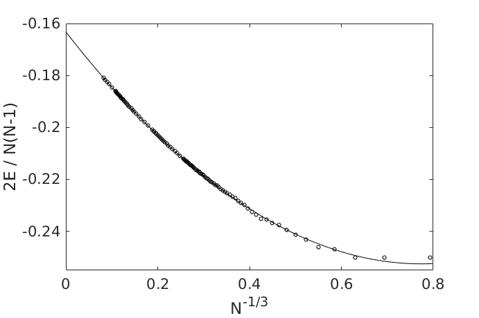
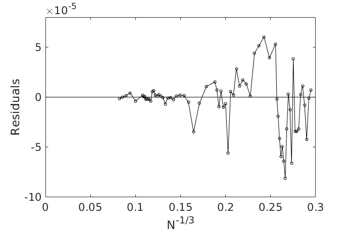
Figure 1: The average energy per particle pair, $\langle E_{2}\rangle$, as a function of $N^{-1/3}$. The line is the fitted cubic polynomial in $N^{-1/3}$ given in Eq. (49). The panel to the right shows the residuals of the fit for $N\geq 39$. It shows magic numbers at $N=250$, $N=120$, and $N=53$.

Since the minimum energy of one particle pair is $-1/4$ at a distance of $d=2$, it is clear that $\langle E_{2}\rangle\geq-1/4$. Obviously, this is a strict inequality for $N>4$, since not all particle pairs can have the optimal distance $d=2$.

The figure shows a slow increase of $\langle E_{2}\rangle$ with $N$. It also shows the existence of “magic numbers”, where the energy is exceptionally low because the particles are arranged in configurations of high symmetry. Some magic numbers are 4 (a regular tetrahedron), 6 (a regular octahedron), 13 (a regular icosahedron with a central particle), 26, and 53. In Section 4 we will show the configurations with $N=26$ and $N=53$.

The average energy per particle pair is well fitted over the whole range, down to $N=2$, by a cubic polynomial in $N^{-1/3}$,

$$E_{2}^{\textrm{fit}}=a_{0}+a_{1}N^{-1/3}+a_{2}N^{-2/3}+a_{3}N^{-1}\;,$$ (49)

with the following values of the coefficients,

$$a_{0}=-0.1632304\;,\quad a_{1}=-0.2270268\;,\quad a_{2}=0.1399513\;,\quad a_{3}=0.0055762\;.$$ (50)

It must be noted that we have done a weighted least squares fit with weights $N^{2}$, because the important point is to obtain a good fit to the energies at the largest values of $N$. Nevertheless the fit is reasonably good all the way down to $N=2$.

The fit gives us a limiting value as $N\to\infty$ which is

$$\langle E_{2}\rangle_{\infty}=a_{0}=-0.1632304\;.$$ (51)

This can be compared to the number computed by Monte Carlo from the Lane–Emden distribution, as given in the appendix,

$$\langle E_{2}\rangle_{\textrm{LE}}=-0.16253\pm 0.00015\;.$$ (52)

We understand the existence of this limit as a consequence of the virial theorem. The energy of one configuration is

$$E=\sum_{\mbox{all pairs}}\left(\frac{1}{d^{2}}-\frac{1}{d}\right),$$ (53)

where $d$ is the distance between the particles of one pair. After $E$ has been minimized, the virial theorem must hold, which says that

$$\sum\left(\frac{2}{d^{2}}-\frac{1}{d}\right)=0\;.$$ (54)

In the last sum, the quantity in parenthesis is positive for $d<2$ and negative for $d>2$. The sum can be zero only if the interparticle distances $d$ are distributed equally below and above $d=2$, as shown in Fig. 2, where we have plotted the contributions to the sum from the different values of $d$. This balance fixes the geometrical size of the cloud of particles. As we increase $N$ the size must remain nearly constant, and all that happens, roughly speaking, is that the density of particles increases everywhere in the same proportion.

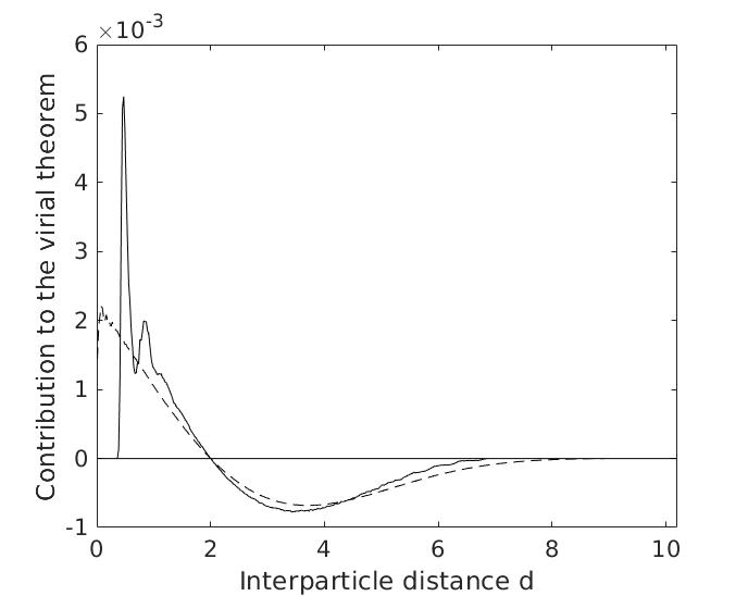
Figure 2: This plot shows how different values of the interparticle distance $d$ contribute to the virial theorem, Eq. (54). The contribution is positive for $d<2$ and negative for $d>2$. The fulldrawn, peaked curve is for 1800 particles in our model. The dashed, smoother curve is for 10 000 independent points drawn at random from the Lane–Emden density distribution. This curve should be essentially independent of the number of points. For the sake of the comparison, both curves are divided by the number of particle pairs.

3.3 Finite size effects

Figure 2 demonstrates clearly how a finite system is different from the continuum limit, in particular because there is a lower limit to the distance between particles. In order to understand the limit $N\to\infty$, we have studied what happens when $N$ increases.

We define $\langle r\rangle$ as the root mean square distance of the particles from the origin. We write $d$ for the distance between two particles, and write $\langle d\rangle$ for the average of $d$ over all the particle pairs. The mean values $\langle r\rangle$ and $\langle d\rangle$ are tabulated in Table 2 for some values of $N$.

$N$	$\langle r\rangle$	$\langle d\rangle$		$N$	$\langle r\rangle$	$\langle d\rangle$
10	1.532 947 447 00	2.223 550 231 57		500	2.408 216 555 94	3.195 863 786 49
20	1.746 229 728 92	2.424 671 301 48		600	2.432 871 960 05	3.227 071 970 79
30	1.852 246 091 36	2.535 394 051 13		625	2.438 273 052 75	3.233 930 049 01
40	1.926 089 543 71	2.617 026 807 14		700	2.452 576 067 99	3.252 214 640 82
56	2.006 652 372 32	2.708 188 019 60		800	2.469 284 455 65	3.273 392 872 15
70	2.059 629 841 53	2.769 512 183 49		1000	2.495 284 325 54	3.306 661 605 26
80	2.087 918 877 46	2.802 950 867 71		1200	2.515 646 479 04	3.332 774 038 07
120	2.170 644 712 76	2.902 144 797 17		1400	2.531 895 026 75	3.353 666 514 75
350	2.356 905 374 94	3.131 156 455 70		1600	2.545 429 383 56	3.371 090 162 89
400	2.376 865 330 71	3.156 148 941 84		1800	2.556 902 476 51	3.385 898 613 04
450	2.393 687 080 41	3.177 398 870 61

Table 2: The root mean square radius $\langle r\rangle$ and the mean distance between particles, $\langle d\rangle$, for the minimum energy configuration of $N$ particles without rotation.

The tabulated data are plotted in the Figures 3 and 4. The curves in the figures are cubic polynomials in $N^{-1/3}$,

$$r_{m}=b_{0}+b_{1}N^{-1/3}+b_{2}N^{-2/3}+b_{3}N^{-1}\;,$$ (55)

and

$$d_{m}=c_{0}+c_{1}N^{-1/3}+c_{2}N^{-2/3}+c_{3}N^{-1}\;,$$ (56)

with the following fitted values for the coefficients,

$$b_{0}=2.86513\;,\quad b_{1}=-3.99618\;,\quad b_{2}=3.13506\;,\quad b_{3}=-1.51269\;,$$ (57)

and

$$c_{0}=3.78972\;,\quad c_{1}=-5.30190\;,\quad c_{2}=4.87658\;,\quad c_{3}=-1.54528\;.$$ (58)

The least squares fitting is done with weight $N$ for each data point, emphasizing the high values of $N$. Also plotted are the residuals $\langle r\rangle-r_{m}$ and $\langle d\rangle-d_{m}$. They show no systematic dependence on $N$. According to the fits there exist limiting values as $N\to\infty$,

$$\langle r\rangle_{\infty}=b_{0}=2.86513\;,\qquad\langle d\rangle_{\infty}=c_{0}=3.78972\;.$$ (59)

These can be compared to the numbers computed by Monte Carlo from the Lane–Emden distribution, as given in the appendix,

$$\langle r\rangle_{\textrm{LE}}=2.9220\pm 0.0029\;,\qquad\langle d\rangle_{\textrm{LE}}=3.8432\pm 0.0037\;.$$ (60)

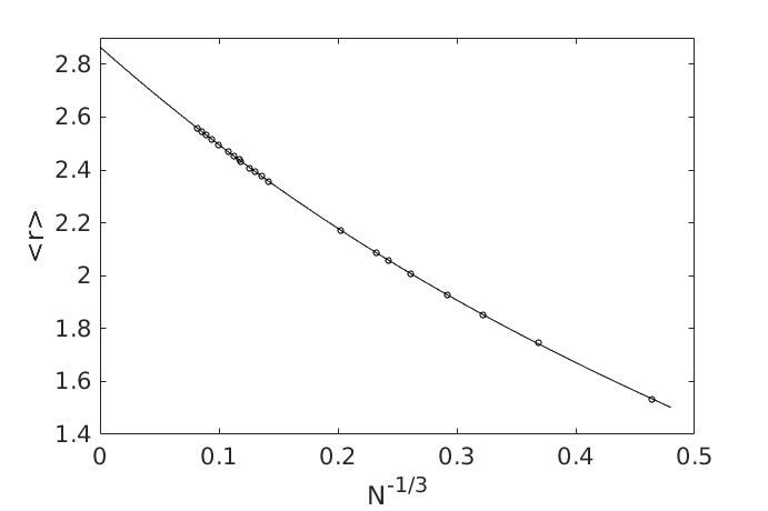
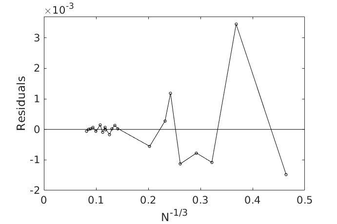
Figure 3: The root mean square radius $\langle r\,\rangle$ as a function of $N^{-1/3}$. The line is the cubic polynomial $r_{m}$ given in Eq. (55). The panel to the right shows the residuals of the fit, $\langle r\rangle-r_{m}$.

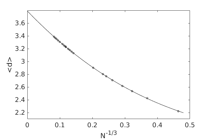
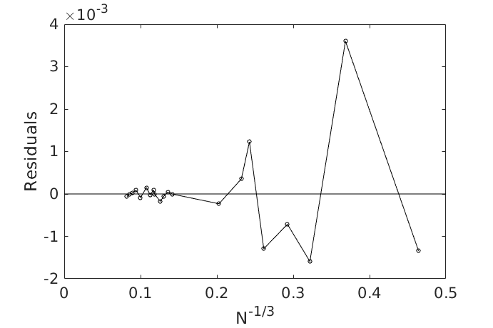
Figure 4: The mean interparticle distance $\langle d\,\rangle$ as a function of $N^{-1/3}$. The line is the cubic polynomial $d_{m}$ given in Eq. (56). The panel to the right shows the residuals $\langle d\rangle-d_{m}$.

Approximate scaling

Figure 5 shows the cumulative distribution of the interparticle distance $d$ for all the particle pairs. The three cases $N=120$, $N=800$, and $N=1800$ are shown, together with the presumed $N\to\infty$ limit given by the Lane–Emden equation. Remember that one particle pair has its minimum energy when $d=2$. Most of the distances are larger, we see for example from figure 5 that for $N=1800$ we have $d>2$ for 90 % of the particle pairs. In the virial theorem, Eq. (54), the 10 % of the distances smaller than two weigh up for the 90 % of the distances larger than two.

All four distributions are seen to have very nearly the same shape. In fact, they are brought to lie very nearly on top of each other when the three configurations with $N=120$, $N=800$, and $N=1800$ are magnified by factors of $1.3243$, $1.1741$, and $1.1351$, respectively. These factors are calculated from the mean values in Table 2, and from the mean value $\langle d\rangle=3.8432$ for the Lane–Emden case, see Appendix B.

The curves can not have identically the same shape, however, for one very good reason. A simple scaling of all the distances $d$ by a common factor would break the virial theorem, because the two terms in Eq. (54) scale differently. It follows that the four curves in Fig. 5 must be visibly different after scaling. The differences in shapes are seen in Fig. 6 at both ends of the curves, while the middle parts of the curves follow each other closely.

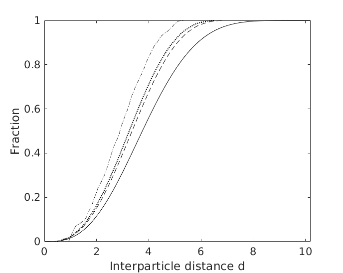
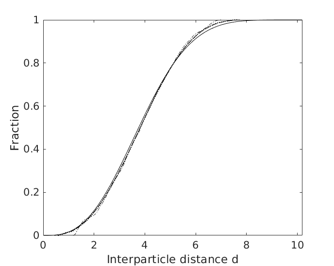
Figure 5: Cumulative distribution of the interparticle distance $d$ for the Lane–Emden distribution (solid line), and our model with $N=1800$ (dashed line), $N=800$ (dotted line), and $N=120$ (dash-dot line). The panel to the right shows that all curves fall very nearly on top of each other when all distances are multiplied by scale factors of $1.1351$ for $N=1800$, $1.1741$ for $N=800$, and $1.3243$ for $N=120$, to make the mean values $\langle d\rangle$ equal.

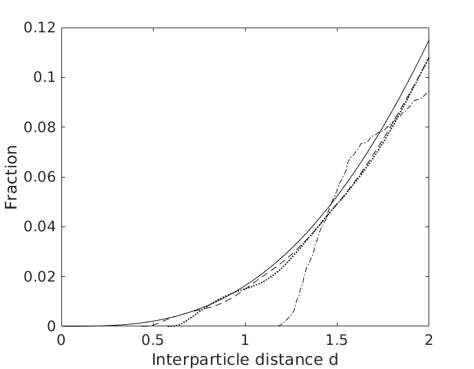
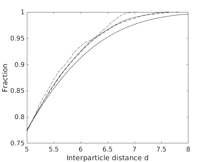
Figure 6: The left panel shows details of the lower part of the right panel in Fig. 5, and the right panel shows the top part of the same figure. We see that with a small number of particles the distribution of interparticle distances is cut off both at small and large values. These cutoffs seem to have little effect on the overall density distribution computed by smearing out the particles artificially, as shown in Fig 7.

Density profiles

The dimensionless Lane–Emden equation, Eq. (95), describes the density profile of a nonrotating polytropic gas cloud of given polytropic index $n$. We take here $n=3/2$. The density at a radius $r=a\xi$ is

$$\rho(r)=\rho_{c}\,(\theta(\xi))^{n}\;,$$ (61)

where $\rho_{c}$ is the central density and $a$ is a scaling factor. The solid curves in the two plots in Fig. 7 show the dimensionless density $\theta^{n}=\rho/\rho_{c}$ as a function of the dimensionless radius $\xi$. The surface of the gas cloud where $\theta(\xi)=0$, is given by $\xi=\xi_{1}=3.653\,754$. The dashed curves in these plots show the density profiles we compute for $N=120$ (left) and $N=1800$ (right). In order to compute a continuous density profile from a configuration of $N$ point particles, we can imagine looking through an unfocused telescope, seeing each point particle as a spherically symmetric gaussian density distribution. We take the standard deviation to be $1.36$, comparable to the minimum distance between points for $N=120$, as Fig. 6 shows, In order to make our numerical density profiles coincide with the theoretical profile for a polytrope, we have to divide $r$, the distance from the origin to a point where we compute the density, by a scale factor $a$ that is $1.485$ for $N=120$ and $1.64$ for $N=1800$. The artificial smearing out of the point particles produces extra tails to the dashed curves.

These plots of density profiles are again good evidence that the configurations of finite numbers of point particles that we generate, can be understood as representing polytropes of index $n=3/2$.

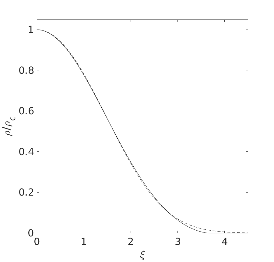
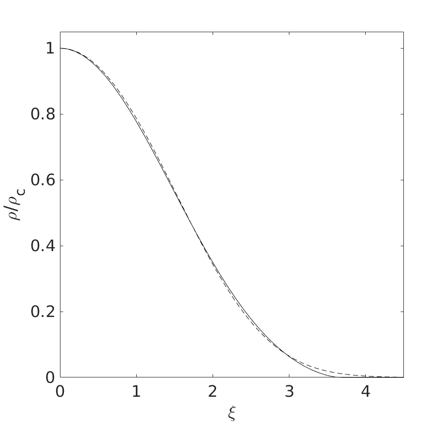
Figure 7: The solid curve in each plot shows the dimensionless density $\theta^{n}$ for $n=3/2$, determined by the Lane–Emden equation, as a function of the dimensionless radius $\xi$. The physical radius is $r=a\xi$ where $a$ is a scale factor. The dashed curve in the left panel is calculated from our nonrotating configuration of 120 point particles, as explained in the text, with a scale factor $a=1.485$. The dashed curve in the right panel is for 1800 particles, here $a=1.64$.

4 Configurations of few particles without rotation

In this section we will describe some of the simplest examples of minimum energy configurations, including the magic numbers $N=26$ and $N=53$.

Five, six, and seven particles. Figure 8 shows the minimum energy configuration of seven particles. With five, six, or seven particles, two of the particles define a symmetry axis, the $z$-axis in the figure. The remaining particles form a regular polygon in the horizontal plane, the $xy$-plane in the figure, an equilateral triangle when $N=5$, a square when $N=6$, or a regular pentagon as in Fig. 8. The configuration with six particles (not shown) has maximal symmetry, since it is a regular octahedron, symmetric under a group of 48 different rotations and reflections.

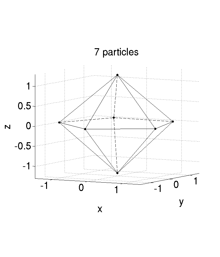
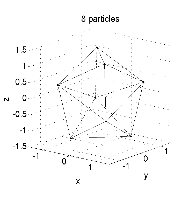
Figure 8: Minimum energy configurations.

Eight particles. The minimum energy configuration of eight particles, also shown in Fig. 8, can be described as made out of two paper boats, where one is turned upside down, rotated $90^{\circ}$ and put on top of the other. It is a polytope with four four-fold corners (where four edges meet), and four five-fold corners. It has a special symmetry which is a simultaneous reflection in the $xy$-plane and a rotation by $90^{\circ}$. It also has two vertical symmetry planes (through the $z$-axis).

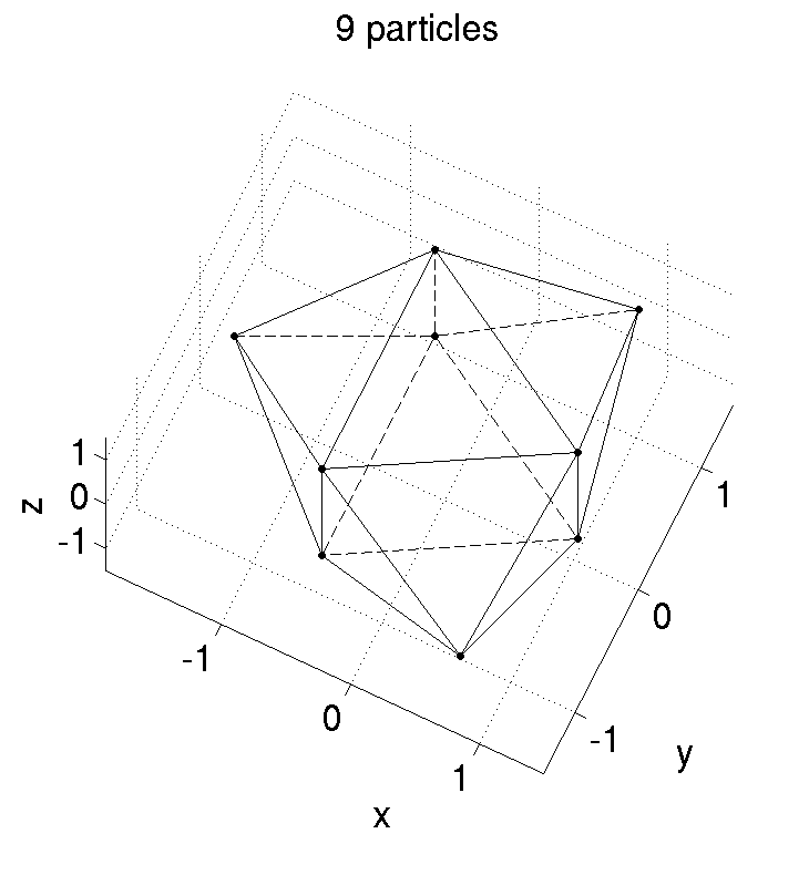
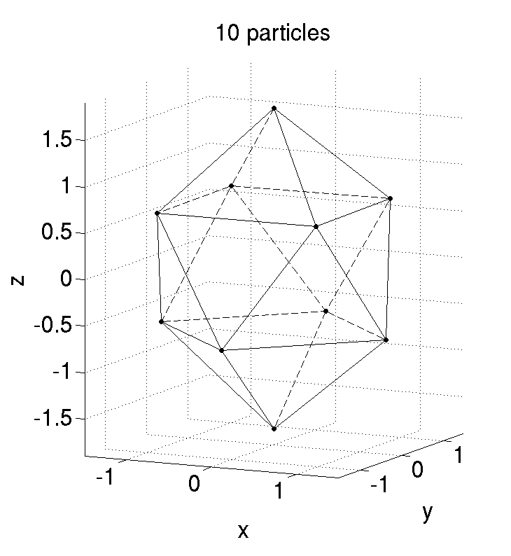
Figure 9: Minimum energy configurations.

Nine particles. The minimum energy configuration with nine particles is shown in Figure 9. It is a polytope with three four-fold and six five-fold corners. It is symmetric under rotations by $120^{\circ}$ about the $z$ axis. The horizontal plane ($xy$-plane) and three vertical planes are symmetry planes.

Ten particles. With ten particles there are two widely different configurations that are nearly degenerate in energy, see Table 1. The one with lowest energy is shown in Fig. 9. It has two four-fold and eight five-fold corners. It has a special symmetry which is a simultaneous reflection in the horizontal plane and a rotation by $45^{\circ}$. It also has four vertical symmetry planes.

The second stable configuration with ten particles, with slightly higher energy, is just the nine-particle configuration shown in Fig. 9 with a tenth particle in the centre. This is actually the first time we encounter a minimum energy configuration with a central particle. It is also the first time we encounter two nearly degenerate minimum energy configurations.

11 particles. The configuration with eleven particles is simply the one with ten particles shown in Fig. 9 with the eleventh particle in the centre.

12 particles. The minimum energy configuration with twelve particles is shown in Fig. 10, It has one central particle at $x=y=0$ and $z=0.034$, slightly above the horizontal plane because this is not a symmetry plane. The only symmetries are reflection symmetries about the $xz$- and $yz$-planes. The top corner is six-fold. Two corners adjacent to this are four-fold, and the remaining eight corners are five-fold.

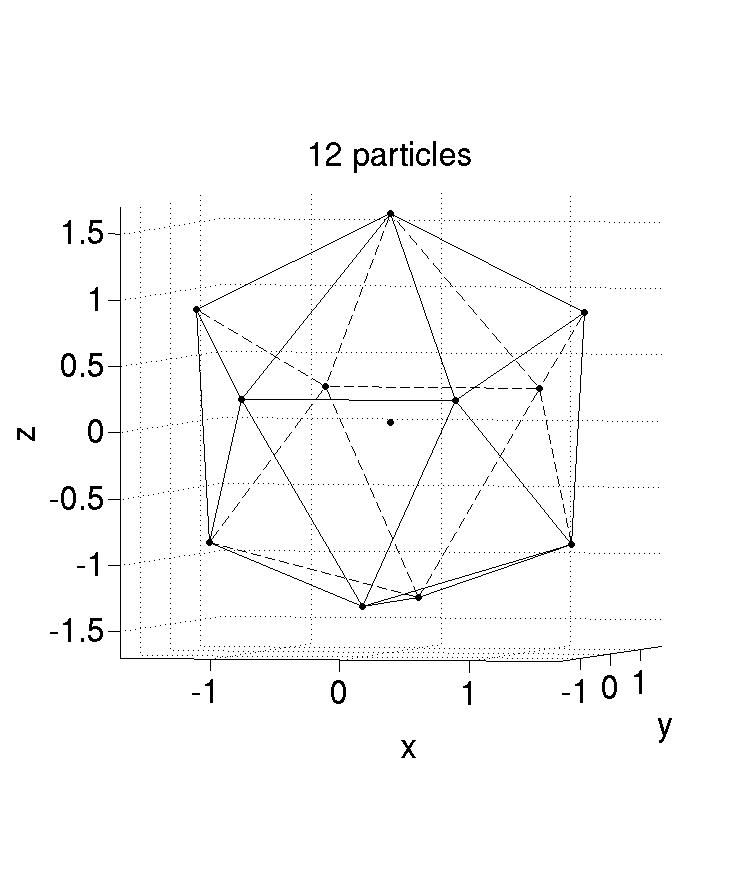
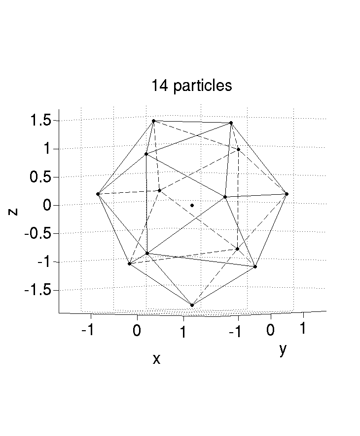
Figure 10: Minimum energy configurations.

13 particles. The minimum energy configuration with thirteen particles is one of the few that have maximal symmetry. It is a regular icosahedron with the thirteenth particle in the centre.

14 particles. In Fig. 10 we show also the configuration with fourteen particles. The bottom corner is four-fold, and the remaining twelve corners are five-fold. Again the central particle is not exactly at the centre, because the horizontal plane is not a symmetry plane. The only symmetry is a $180^{\circ}$ rotation about the $z$-axis.

15 particles. In Fig. 11 we show the configuration of fifteen particles. The central particle is exactly at the centre. The top and bottom corners are six-fold, and the remaining twelve corners are five-fold. A simultaneous reflection about the horizontal plane and a rotation by $30^{\circ}$ about the $z$-axis is a symmetry. In addition there are six vertical symmetry planes.

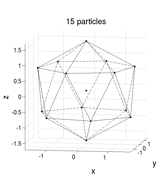
Figure 11: Minimum energy configuration with a particle exactly at the centre.

26 particles. In Fig. 12 we show the “magic” configuration of 26 particles. This has an exceptionally low energy because of its high symmetry, which is not obvious from the complete figure, although the projections onto the $xy$-, $xz$- and $yz$-planes are equal and highly symmetric. There is a central regular tetrahedron, and the symmetry group of the whole configuration consists of all the 24 permutations of the corners of this tetrahedron. The tetrahedron is surrounded by a shell made up of three different polyhedra with the same tetrahedral symmetries, shown here in the same figure. One contains 12 particles and can be understood as a cube with all six corners cut off. The other two are a regular octahedron and a regular tetrahedron

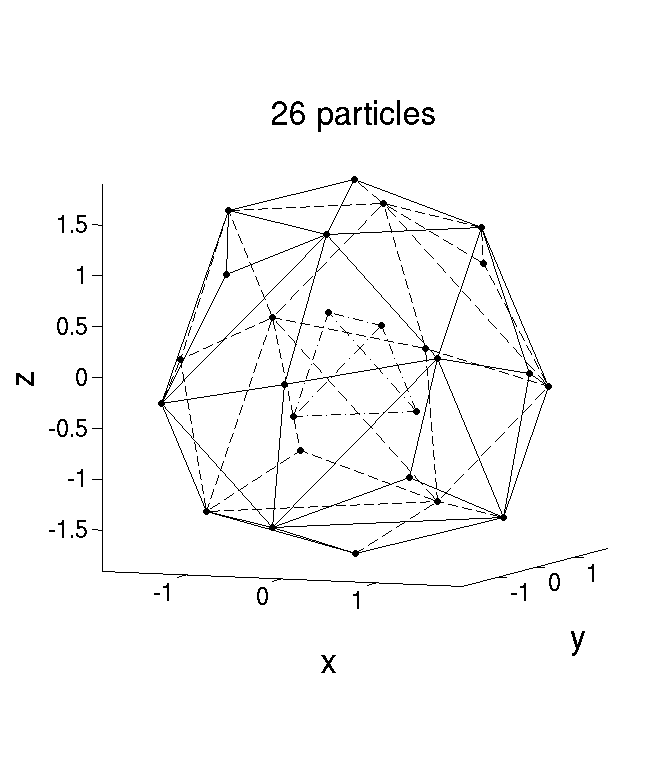
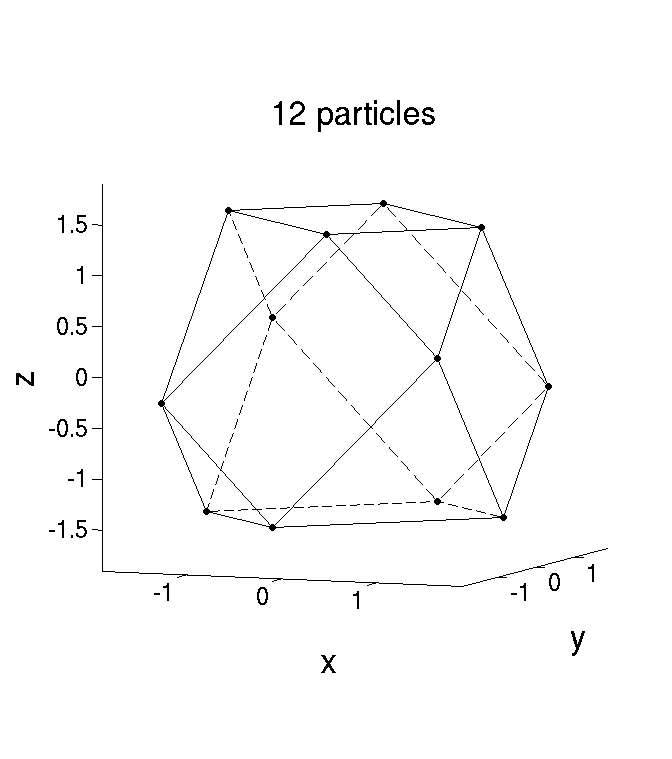
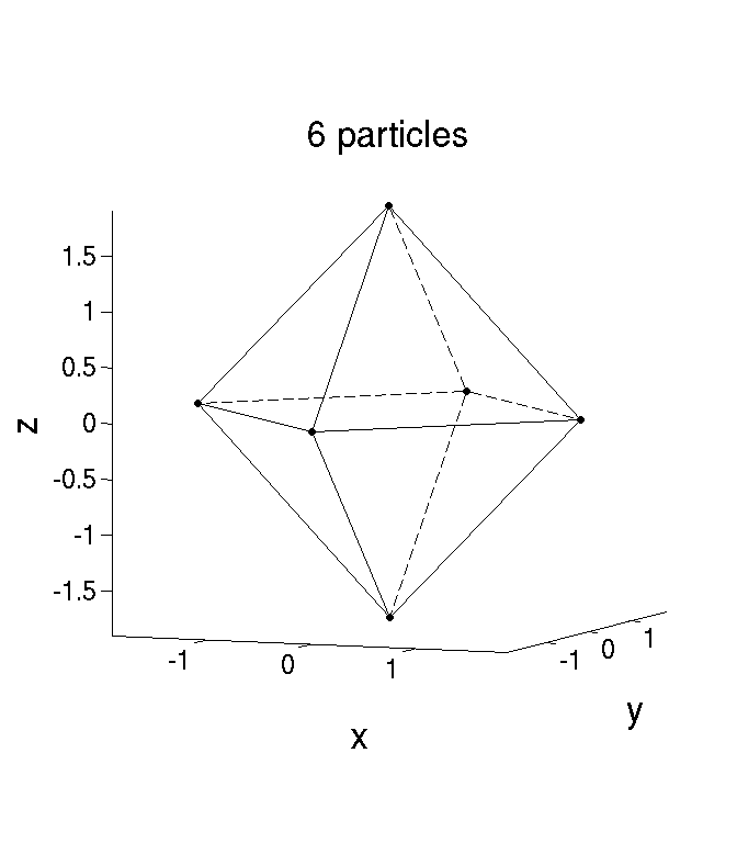
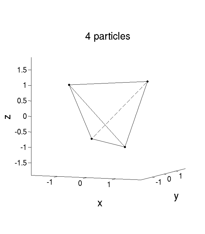
Figure 12: Minimum energy configuration with 26 particles, consisting of an inner tetrahedron and and an outer shell made up of three simple polyhedra.

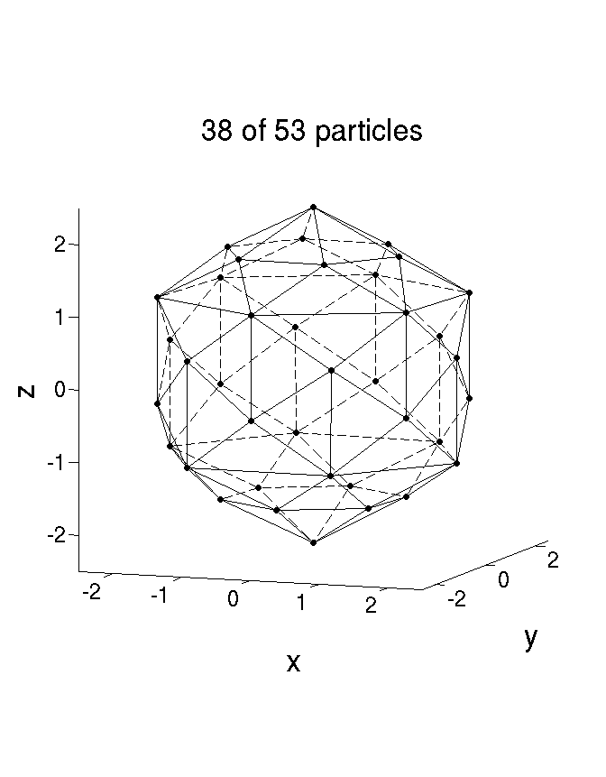
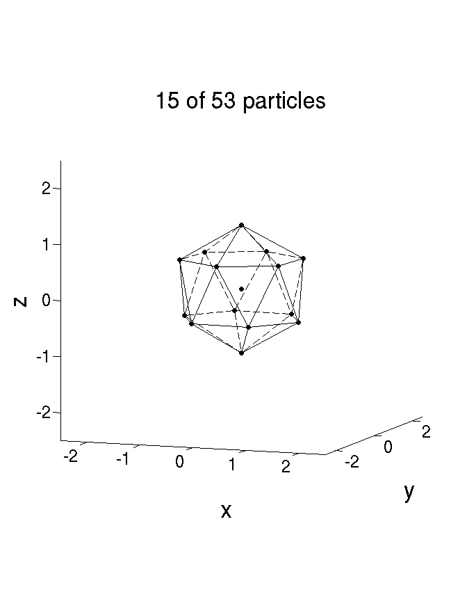
Figure 13: Minimum energy configuration with 53 particles. There is one central particle, an inner shell of 14 particles (right), and an outer shell of 38 particles (left),

53 particles. In Fig. 13 we show the configuration of 53 particles, another “magic” case. There is one central particle exactly at the centre, and two concentric approximately spherical shells, plotted separately in the figure. The inner shell contains 14 particles and has a root mean square radius of $1.211\,011\,415\,841$. The outer shell contains 38 particles and has a radius of $2.237\,680\,879\,671$. The inner shell plus the central particle is like the configuration of 15 particles plotted in Fig. 11, compressed by a factor of $0.71$. In fact, the root mean square radius of the shell in Fig. 11 is $1.707\,609\,454\,071$.

A complete description of the configuration of 53 particles is given in Table 3. Five particles lie along the $z$-axis, while 48 particles form regular hexagons centered on the $z$-axis in eight planes perpendicular to the $z$-axis. The hexagons in adjacent planes are rotated $30^{\circ}$ relative to each other. In the table, $r_{2}$ is the distance of the points from the $z$ axis (the radius of the hexagons), and $r_{3}$ is the distance from the origin. The basic symmetry transformation is a simultaneous rotation by $30^{\circ}$ about the $z$-axis and a reflection about the $xy$-plane. In addition, there are six vertical symmetry planes.

$z$	$r_{2}$	$r_{3}$
$0.0\phantom{00\,000\,000\,000}$	$0.0\phantom{00\,000\,000\,000}$	$0.0\phantom{00\,000\,000\,000}$
$\pm 1.140\,738\,013\,178$	$0.0\phantom{00\,000\,000\,000}$	$1.140\,738\,013\,178$
$\pm 2.304\,942\,769\,817$	$0.0\phantom{00\,000\,000\,000}$	$2.304\,942\,769\,817$
$\pm 0.360\,452\,820\,441$	$2.138\,438\,168\,526$	$2.168\,604\,167\,747$
$\pm 0.535\,171\,243\,082$	$1.098\,947\,054\,672$	$1.222\,330\,924\,257$
$\pm 1.098\,246\,666\,131$	$2.135\,949\,636\,872$	$2.401\,754\,898\,178$
$\pm 1.697\,413\,737\,050$	$1.272\,100\,190\,070$	$2.121\,191\,242\,746$

Table 3: The minimum energy configuration for $53$ particles without rotation. $r_{2}$ and $r_{3}$ are defined in the text.

5 Rotating systems of finite numbers of point particles

So far we have studied nonrotating minimum energy configurations, arguing that they can represent polytropes of index $n=3/2$, as described by the Lane–Emden equation. In particular, we have shown that already with 120 point particles they reproduce very well the polytropic density profile. We will now show how they become deformed when set into rotation.

In contrast to a liquid of constant density, a polytrope is compressible. It has a sharply defined surface, like the liquid, but its density goes to zero at the surface. Jeans [8, 9, 10] concluded that the compressibility implies that the transition from a Maclaurin ellipsoid, having a circular shape in the plane perpendicular to the rotation axis, to a Jacobi ellipsoid, having three different principal axes, can take place with a rotating polytrope only when the polytropic index $n$ is smaller than a critical value $n_{c}\approx 0.83$. This value was confirmed by James [12], who found $n_{c}\approx 0.808$. See Appendix A for a summary of the reasoning of Jeans.

It means that we can not expect to see the Maclaurin to Jacobi transition in our simulations with $n=1.5$. What happens instead, before the bifurcation point is reached, is that the rotating polytrope becomes unstable by shedding particles at the equator, where the centrifugal force exactly balances the gravitational attraction. This balance implies that the equator becomes a sharp edge, as described by Jeans. In our simulations, as presented here, we see clearly this sharp edge appearing when the angular momentum reaches its maximal value.

5.1 The maximal angular momentum

We have tried to determine with good precision, for some values of $N$, the maximal value $L_{\textrm{max}}$ that the angular momentum $L$ can take before the system becomes unstable by losing particles. The results are summarized in Table 4 and Fig, 14. The figure shows that the data follow very closely the power law

$$L_{\textrm{max}}=aN^{b}\;,$$ (62)

with $a=0.30157$ and $b=1.5510$.

$N$	$L_{\textrm{max}}$	$W_{\textrm{max}}$
005	$\phantom{000}8$	$0.1876$
010	$\phantom{00}10$	$0.0733$
015	$\phantom{00}21$	$0.0804$
020	$\phantom{00}34$	$0.0827$
025	$\phantom{00}46$	$0.0757$
050	$\phantom{0}130$	$0.0647$
100	$\phantom{0}345$	$0.0595$
150	$\phantom{0}715$	$0.0681$
200	$1140$	$0.0701$
400	$3348$	$0.0711$
700	$7895$	$0.0713$

Table 4: The maximal angular momentum $L_{\textrm{max}}$ for different numbers of particles, and the corresponding $W$ values. Note the drop in $W_{\textrm{max}}$ from $N=5$ to $N=10$.

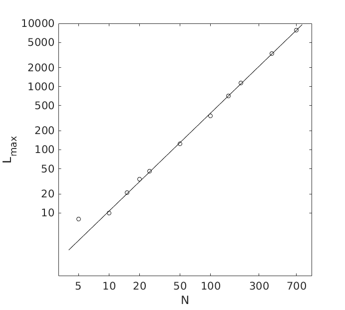
Figure 14: The numerical values of $L_{\textrm{max}}$ given in Table 4. The straight line is the power law given in Eq. (62).

We can understand the power $b\approx 1.5$ in the following way. In the virial theorem, Eq. (18), we have for large $N$ that the first two terms are proportional to the number of particle pairs, $N(N-1)/2$,

$$U_{\textrm{rep}}=AN^{2}\;,\qquad V_{\textrm{grav}}=-BN^{2}\;,$$ (63)

with positive coefficients $A$ and $B$ that do not vary much with $N$. In the rotational energy $E_{\textrm{rot}}=L^{2}/(2I)$, the moment of inertia is proportional to the number of particles,

$$I=CN\;,$$ (64)

with a coefficient $C$ that is again nearly independent of $N$. Thus the virial theorem implies that

$$L=\sqrt{C(B-A)N^{3}}\;.$$ (65)

This argument would imply that $b\to 1.5$ in the limit $N\to\infty$.

5.2 The ratio between rotational and gravitational energy

The table also gives the maximal value $W_{\textrm{max}}$ of the ratio between the rotational energy and the gravitational energy, $W=E_{\textrm{rot}}/|V_{\textrm{grav}}|$. This maximal value is known to be smaller for a polytrope than for a liquid of constant density [20]. It is an interesting result we obtain that the value of $W_{\textrm{max}}$ seems to be roughly independent of the number of particles.

The virial theorem gives Eq. (20),

$$W=\frac{E_{\rm rot}}{|V_{\rm grav}|}=\frac{1}{2}-\frac{U_{\rm rep}}{|V_{\rm grav}|}\leq\frac{1}{2}\;.$$ (66)

This upper limit of $1/2$ is much larger than the values $W_{\textrm{max}}\approx 0.07$ that we find in our simulations. The exceptional value $W_{\textrm{max}}=0.1876$ listed in the table for five particles is not representative, because it occurs when the particles line up on a straight line, and ${U_{\rm rep}}/{|V_{\rm grav}|}\approx 0.31$, see [1]. The low value $W_{\textrm{max}}\approx 0.07$ corresponds to a much higher value of the repulsive potential, ${U_{\rm rep}}/{|V_{\rm grav}|}\approx 0.43$.

Note that the upper limit of $1/2$ in Eq. (66) is the same as the upper limit for a Maclaurin ellipsoid in the case of an incompressible fluid [20]. We could in principle simulate a nearly incompressible fluid by inserting a very large value for the power $k=3(\gamma-1)$ in Eq. (8). This would imply a generalized virial theorem, and the following generalization of Eq. (66),

$$W=\frac{E_{\rm rot}}{|V_{\rm grav}|}=\frac{1}{2}-\frac{kU_{\rm rep}}{2\,|V_{\rm grav}|}\leq\frac{1}{2}\;.$$ (67)

We may argue that it would also lead to a small limiting value for ${kU_{\rm rep}}/{|V_{\rm grav}|}$, so that $W$ would approach the limit of $1/2$.

6 Example: 400 particles

We have generated more than 1600 configurations consisting of 400 point particles with different values of the angular momentum. Most of them are generated by following stable branches, increasing or decreasing the angular momentum $L$ in small steps. In this section we present some results obtained from studying these data. For comparison we also present some results for 700 particles, and also some cases of fewer than 400 particles.

The general picture is that with an increasing number of particles the systems we study resemble more and more a continuous polytrope. We confirm the Jeans effect as defined in the introduction, that configurations become unstable at the highest values of $L$ by shedding single particles at the equator, which then becomes a sharp edge. We also see strong evidence for the result obtained by Jeans that a polytrope with polytropic index $n=1.5$ remains rotationally symmetric in the rotation plane until it becomes unstable at $L=L_{\textrm{max}}$.

6.1 Stability

In paper I we studied systems of very few particles, and gave detailed descriptions of how different branches of stable configurations evolve with increasing angular momentum $L$. Obviously, this we can not do here in the same detail, because the number of branches is extremely large. Nevertheless, we can pick at random one branch at a time and follow its evolution, changing $L$ in small steps. In Fig. 15 we plot the stability parameter $\sigma$ for 400 particles, as a function of $L$, for some 40 branches above $L=2800$. Every branch is seen to be stable only in a rather small $L$ interval. We find no stable branches above $L_{\textrm{max}}=3348$.

As an indication of to what degree our random sample of branches is complete, we have searched for, and found, other stable configurations at $L=3067$. These are plotted in the figure as (purple) circles, They indicate that continued searches would reveal a very large number of branches, also in seemingly empty areas in the plot.

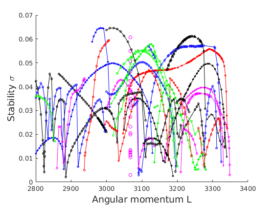
Figure 15: Evolution of the stability parameter $\sigma$ as a function of the angular momentum $L$, for around 40 stable branches of configurations of 400 particles. The isolated circles at $L=3067$, belonging to other branches that we have not followed, indicate that the present sample of branches is very far from complete.

6.2 Asymmetry

In Section 2.5 we defined different asymmetry parameters. In Fig. 16 we see how the asymmetry $A_{12}$, in the rotation plane (the $xy$-plane), increases with $L$. The main result to be noted is that it is small. We believe that the reason for the sharp increase in $A_{12}$ when $L$ comes close to $L_{\textrm{max}}$, is that the number of particles is finite, and single particles at the equator become more and more loosely bound. This is simply what we call the Jeans effect.

In the left panel of Fig. 17 we see how the asymmetry $A_{13}$, in the $xz$-plane, changes as a function of $L$. The right panel shows the asymmetry $A_{23}$, in the $yz$-plane. They are both much larger than the $xy$ asymmetry $A_{12}$. The reason is of course that they measure the rotational flattening, which is large. The smallness of $A_{12}$ in comparison indicates that it may vanish in the continuum limit $N\to\infty$, as predicted by Jeans. For a given value of $L$ approaching $L_{\textrm{max}}$, all three asymmetries, in particular $A_{12}$, show substantial variations.

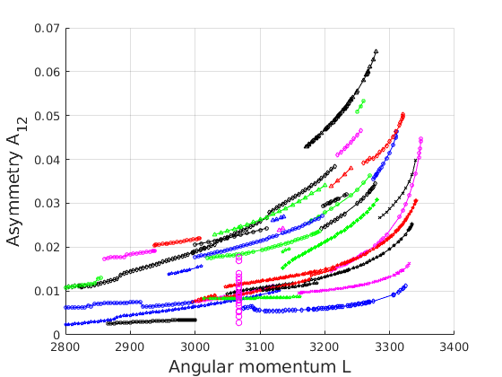
Figure 16: This plot for 400 particles shows how the asymmetry parameter $A_{12}$ increases with the angular momentum $L$. The sample of branches, and the isolated points at $L=3067$, are the same as in Fig. 15.

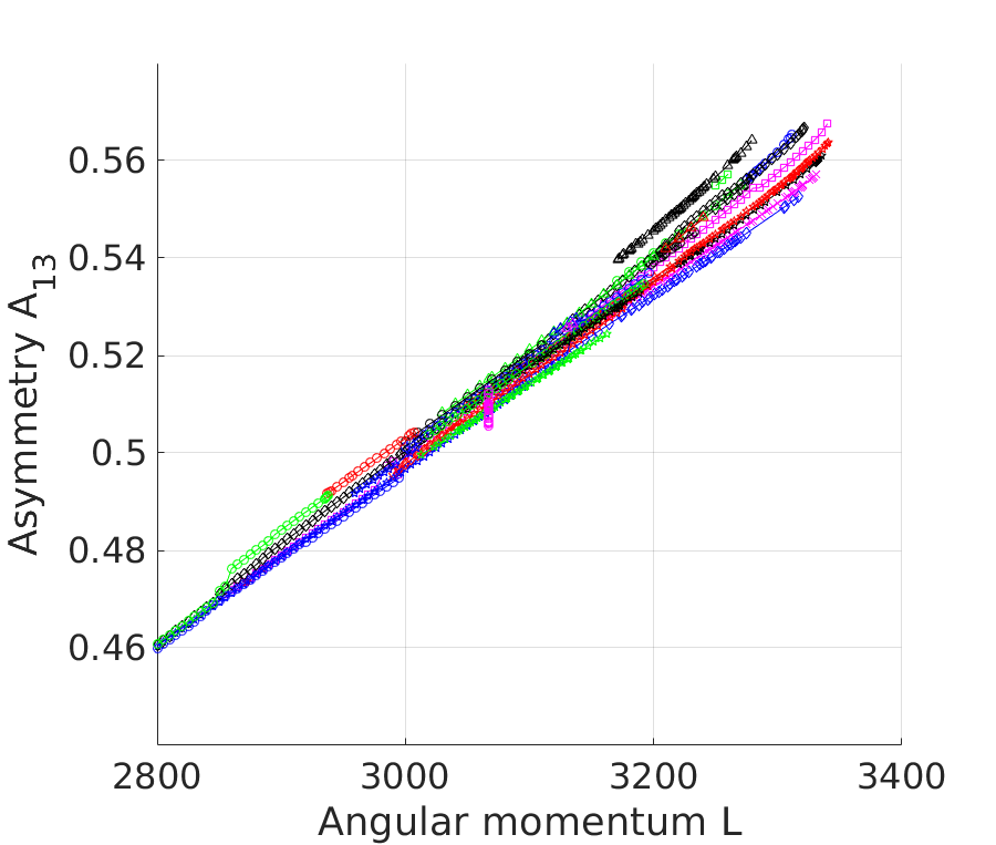
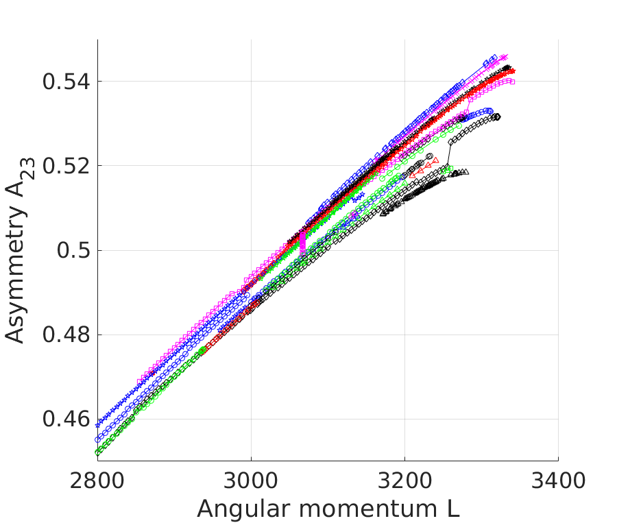
Figure 17: These plots for 400 particles show how the asymmetry parameters $A_{13}$, in the left panel, and $A_{23}$, in the right panel, evolve as functions of the angular momentum $L$ .

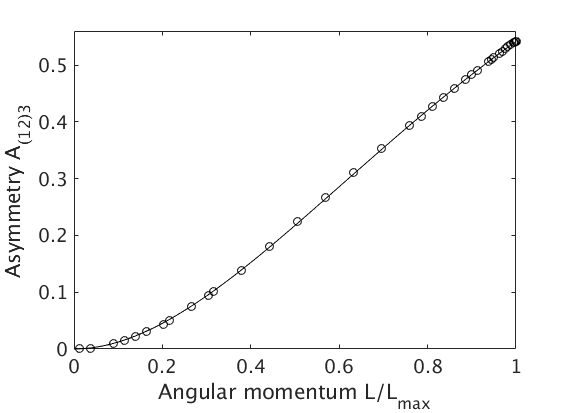
Figure 18: The asymmetry parameter $A_{(12)3}$ as a function of the scaled angular momentum $L/L_{\textrm{max}}$ for 700 particles. Here $L_{\textrm{max}}=7895$. The curve is a quartic polynomial fitted to the data points, see Eq. (68).

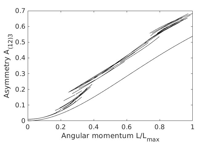
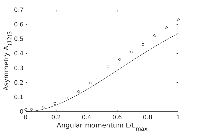
Figure 19: The asymmetry parameter $A_{(12)3}$ as a function of the angular momentum $L/L_{\textrm{max}}$ for 25 particles, with $L_{\textrm{max}}=44.6$, and for 50 particles, with $L_{\textrm{max}}=130$. The curve in both plots is the quartic polynomial fitted to the data for 700 particles.

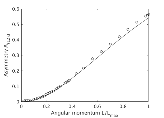
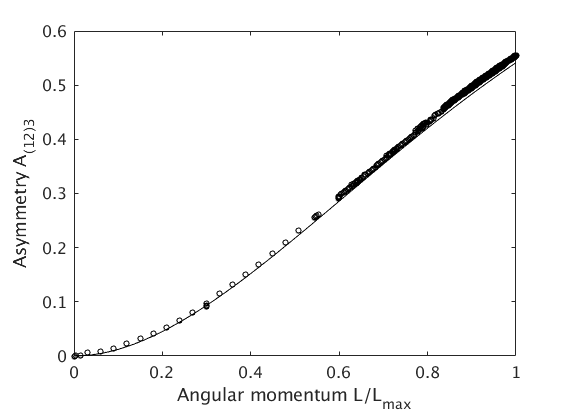
Figure 20: The asymmetry parameter $A_{(12)3}$ as a function of the angular momentum $L/L_{\textrm{max}}$ for 150 particles, with $L_{\textrm{max}}=715$, and for 400 particles, with $L_{\textrm{max}}=3348$. The curve is the fit for 700 particles.

It follows from Eq. (40) that $A_{13}=A_{23}$ if $A_{12}=0$, and that $A_{13}>A_{23}$ if $A_{12}>0$. Since we have $A_{12}>0$ in our data, and expect that $A_{12}=0$ in the continuum limit, we conclude that the proper asymmetry to study in the limit is neither $A_{13}$ nor $A_{23}$, but rather $A_{(12)3}$ as defined in Eq. (41). This is plotted in Fig. 18 for 700 particles, together with a fitted curve which is the following quartic polynomial,

$$A_{\textrm{fit}}=c_{2}\left(\frac{L}{L_{\textrm{max}}}\right)^{\!2}+c_{3}\left(\frac{L}{L_{\textrm{max}}}\right)^{\!3}+c_{4}\left(\frac{L}{L_{\textrm{max}}}\right)^{\!4}\;,$$ (68)

with $L_{\textrm{max}}=7895$ and with

$$c_{2}=1.33288\;,\qquad c_{3}=-1.05954\;,\qquad c_{4}=0.26853\;.$$ (69)

We have assumed in the fit that the asymmetry grows quadratically with $L$ for small $L$. The fit is remarkably good with as few as three parameters.

The Figures 19 and 20 show the same asymmetry $A_{(12)3}$ as a function of $L/L_{\textrm{max}}$ for 25, 50, 150, and 400 particles, compared to the curve fitted for 700 particles. It is worth noting that for 400 particles, where we have 1628 data points for $A_{(12)3}$, all these points fall very nearly on one single curve, with fluctuations presumably because there are a finite number of particles. We see in Fig. 17 that $A_{13}$ and $A_{23}$ show larger variations for a fixed value of $L$ (but note the factor of nearly ten between the scales of the plots).

If there does exist a continuum limit when $N\to\infty$ we would expect the asymmetry as a function of $L/L_{\textrm{max}}$ to become independent of $N$ in the limit. These plots show clearly a finite size effect, that the asymmetry decreases when the number of particles increases. We believe that the continuum limit exists, but we have not quite reached it yet.

6.3 The energy as a function of $L$

The left panel in Fig. 21 shows how the average energy per particle pair, $\langle E_{2}\rangle=2E/N(N-1)$, increases with the angular momentum $L$ for 400 particles. The following polynomial of degree five gives an excellent fit,

$$E_{\textrm{fit}}=d_{0}+d_{2}\left(\frac{L}{L_{\textrm{max}}}\right)^{\!2}+d_{3}\left(\frac{L}{L_{\textrm{max}}}\right)^{\!3}+d_{4}\left(\frac{L}{L_{\textrm{max}}}\right)^{\!4}+d_{5}\left(\frac{L}{L_{\textrm{max}}}\right)^{\!5}\;,$$ (70)

with $L_{\textrm{max}}=3348$ and with

$$d_{0}=-0.19146\;,\quad d_{2}=0.04881\;,\quad d_{3}=-0.01170\;,\quad d_{4}=-0.01118\;,\quad d_{5}=0.00556\;.$$ (71)

The fitted value of $d_{0}$, the energy at $L=0$, is the same as the value at $N=400$, $L=0$, given in Table 1.

The right panel in Fig. 21 shows how the ratio of rotational and gravitational energy, $W=E_{\textrm{rot}}/|V_{\textrm{grav}}|$, increases with $L$. We fit it by the following polynomial,

$$W_{\textrm{fit}}=e_{2}\left(\frac{L}{L_{\textrm{max}}}\right)^{\!2}+e_{3}\left(\frac{L}{L_{\textrm{max}}}\right)^{\!3}+e_{4}\left(\frac{L}{L_{\textrm{max}}}\right)^{\!4}+e_{5}\left(\frac{L}{L_{\textrm{max}}}\right)^{\!5}\;,$$ (72)

with

$$e_{2}=0.12960\;,\quad e_{3}=-0.05269\;,\quad e_{4}=-0.02195\;,\quad e_{5}=0.01618\;.$$ (73)

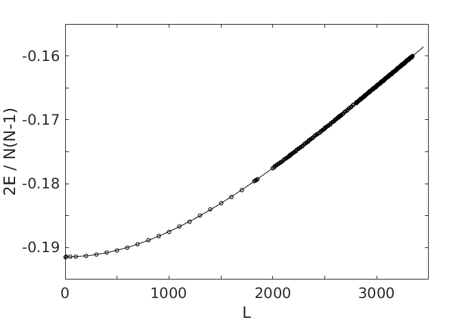
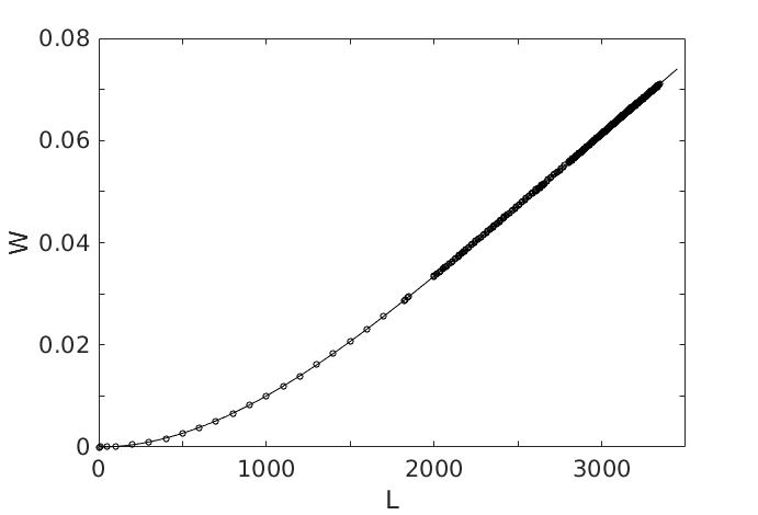
Figure 21: The left panel shows the average energy per particle pair as a function of the angular momentum $L$, for $N=400$. The curve is the fitted polynomial given in Eq. (70). The right panel shows the ratio $W$ as a function of $L$. Again the curve is a polynomial fit, Eq. (72).

6.4 The Jeans effect

The Figures 22, 23, and 24 show configurations of 400 and 700 particles, with one value of the angular momentum below and one value equal to the maximum value. These figures confirm the visible features that we defined in the Introduction as parts of the Jeans effect. They are:

• There is always circular symmetry in the rotation plane.

• Instability at the maximal angular momentum is due to particle loss from the centrifugal force at the equator.

• The equator becomes a sharp edge at the maximal angular momentum.

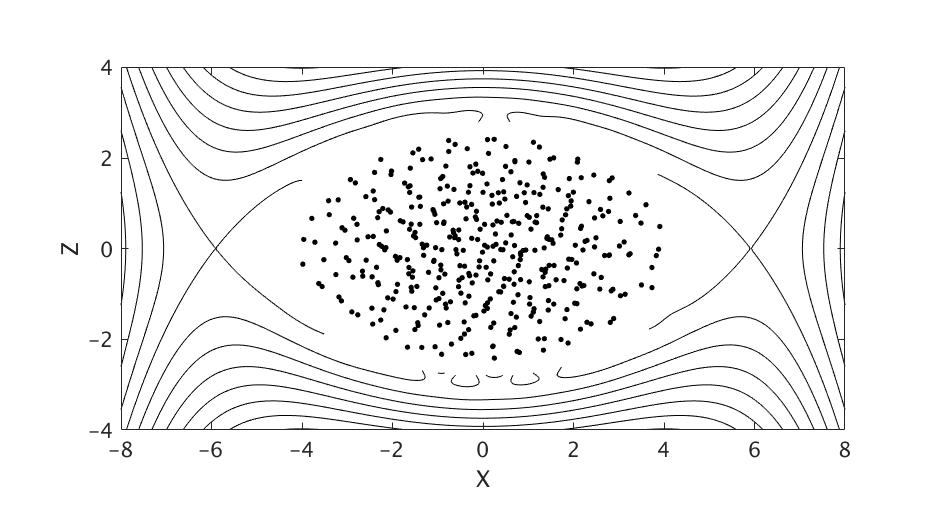
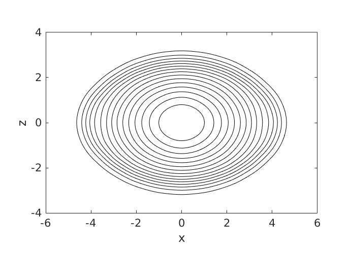
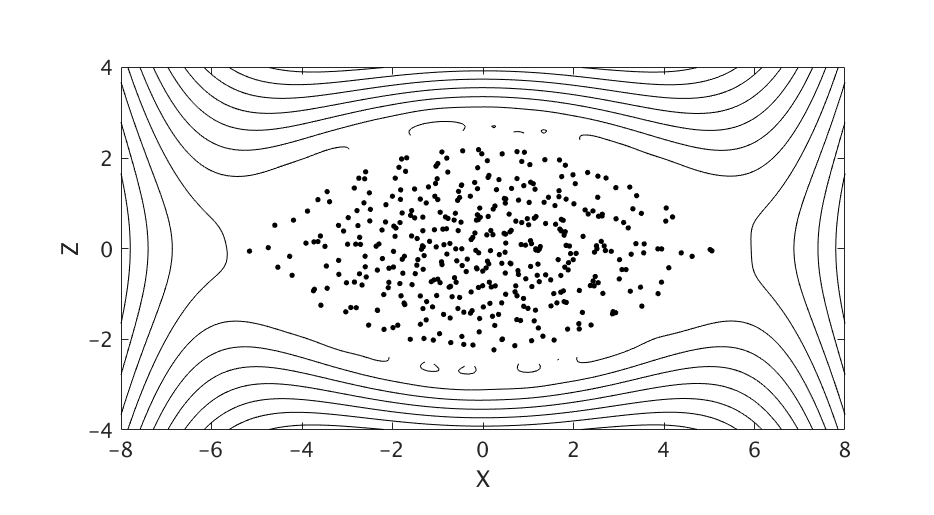
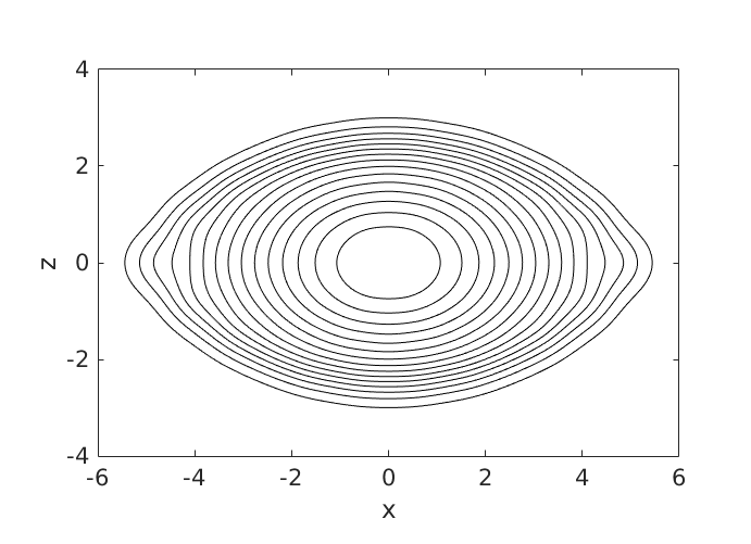
Figure 22: The left panels show the $xz$ projections of two different configurations with 400 particles, at angular momenta $L=2500$ (top) and $L=L_{\textrm{max}}=3348$ (bottom). Also plotted are equipotential lines in the $xz$-plane. The right panels show the same configurations represented as contour curves of the densities in the $xz$-plane. The sharp edge at the equator at the maximum angular momentum is clearly seen.

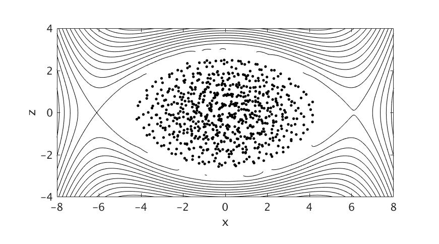
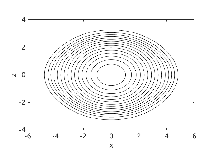
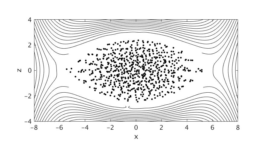
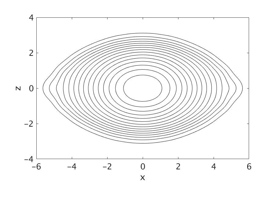
Figure 23: The left panels show the $xz$ projections of two configurations of 700 particles, at $L=6000$ (top) and at $L=L_{\textrm{max}}=7895$ (bottom). The right panels show the same configurations represented as contour curves of the densities. Again the sharp edge at the equator at the maximum angular momentum is clearly seen.

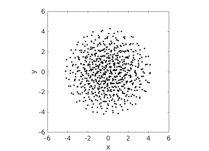
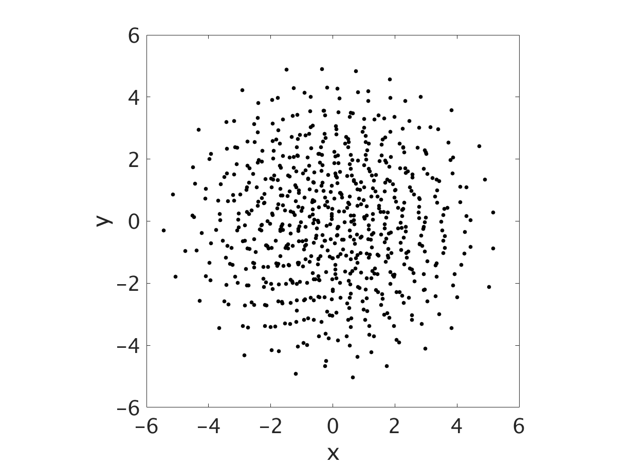
Figure 24: The $xy$ projections of the two configurations in Fig. 23 with 700 particles. In the left panel, we have $L=6000$ and $A_{12}=0.0024$. In the right panel, we have $L=L_{\textrm{max}}=7895$ and $A_{12}=0.021$, here we see that the outer particles in the equator region are very loosely bound. The asymmetry in this projection is too small to be visible.

The potential $\phi$, defined in Eq. (27) and plotted with level curves in the figures, is everywhere negative, it goes to $-\infty$ as $x\to\pm\infty$, and to zero along the $z$-axis as $z\to\pm\infty$. Note the two saddle points (Lagrange points) in each plot, most visible in the top left panels. With the corresponding level curves they delimit the Roche lobe, within which an external particle would be bound. As $L$ increases towards $L_{\textrm{max}}$ the cloud of particles becomes unstable by filling its Roche lobe, developing the sharp edge shaped by the Roche lobe. For $L<L_{\textrm{max}}$ there is no sharp edge. These features are the same for 400 and 700 particles.

We claim that, within their limits, these figures are good representations of the behaviour of a polytropic gas. As shown in Appendix B, the level curves of the pressure and density inside a gravitationally bound polytrope are the same as the equipotential surfaces (of gravitational plus centrifugal potential). It should be remembered, however, that the correspondence between the two different systems has its limits. In particular, the potential plotted in our figures has point sources and is not smooth like the potential from the polytrope, and it includes our artificially introduced short range repulsion potential.

Figure 24 illustrates both the absence of the Jacobi transition, and the instability due to centrifugal forces, as predicted by Jeans. It shows the projections on the rotation plane or $xy$-plane of the two configurations of 700 particles shown in Fig. 23. The configuration in the top panels is at $L=6000$, and has rotational symmetry with no signs of the shedding of particles. The configuration in the bottom panels is at $L=L_{\textrm{max}}=7895$, and we see that the outermost particles clearly are on the brink of drifting away. But despite the fact that the configuration is close to breakup, it remains rather circularly symmetric, thus confirming the Jeans effect.

7 Conclusion and outlook

We have used a model with $N$ particles, where $N$ is a large but finite number, to simulate a gravitationally bound rotating polytrope. We argue that this method is valid, and that the continuum limit can be described as the limit $N^{-1/3}\to 0$.

The method is useful because it is simpler than solving a partial differential equation. Although the continuum limit is approached rather slowly, conclusions can be drawn from values of $N$ of a few hundred, which are tractable numbers.

The polytropic index $n$ corresponds in our model to a repulsive potential between the particles inversely proportional to the distance to the power $3/n$. We have studied only the special case $n=3/2$, corresponding to an inverse square repulsive potential.

One of the problems left for further investigations is to change the value of $n$. A technical problem which then appears is that the virial theorem becomes slightly more complicated, because the three terms in Eq. (17) scale with three different powers of $\alpha$.

In particular, it would be interesting to study the Jacobi transition to a shape which is no longer rotationally symmetric in the rotation plane, and to verify the necessary condition found by Jeans, that $n<0.83$.

In a rather different direction, the method described here could be used for studying rotating molecules, with totally different interaction potentials. The method used for computing stability can be used for computing vibrational frequencies.

Appendix A The Jeans theory of rotationally distorted polytropes

To find out how fast a body that is gravitationally compressed at its centre can rotate before it becomes unstable, Jeans constructed what he called the adiabatic model, described by an equation of state of the form

$$P=K\rho^{\gamma}-p_{0}\;.$$ (74)

We will summarize here very briefly his reasoning and main results. See [8, 9, 10] for more details.

A positive constant $p_{0}$ in the equation of state implies that the density $\rho$ at the surface, where $P=0$, may have a positive value $\sigma$. Physically, it means that the theory may describe an inner part of a larger body. He introduces a compressibiliy parameter

$$\epsilon=\frac{\rho_{c}-\sigma}{\rho_{c}}\;,$$ (75)

where $\rho_{c}$ is the central density. Thus, $\epsilon=0$ corresponds to an incompressible fluid, or the central part of a larger body, whereas $\epsilon=1$ for a polytrope with equation of state $P=K\rho^{\gamma}$.

A slowly rotating incompressible body takes the shape of a Maclaurin ellipsoid, or spheroid, with two equal axes. With faster rotation this becomes unstable, and bifurcates to a Jacobi ellipsoid, with three different axes. The shape of a slowly rotating compressible body will be what Jeans calls a distorted spheroid, or pseudo-spheroid. A main result derived by Jeans is that the bifurcation to a distorted Jacobi ellipsoid will not take place if the adiabatic index $\gamma$ is too small, so that the body is too much centrally condensed. Then it becomes unstable instead by shedding particles at the equator.

Jeans writes the variable density as

$$\rho(x,y,z)=\rho_{c}\,(1-\epsilon F(x,y,z))\;.$$ (76)

The surface is given by the equation $\rho=\sigma$, and with the definition (75) this means that $F=1$. Knowing that the surface is a spheroid in the incompressible case $\epsilon=0$, he then writes

$$F=\frac{x^{2}+y^{2}}{a^{2}}+\frac{z^{2}}{c^{2}}+\epsilon P_{0}+\epsilon^{2}Q_{0}+\epsilon^{3}R_{0}+\cdots\;.$$ (77)

Here $a$ and $c$ are the semiaxes of the spheroid when $\epsilon=0$, and $P_{0},Q_{0},R_{0},\ldots$ are functions of $x,y,z$ describing how the spheroid is distorted when $\epsilon>0$. Expanding to second order in $\epsilon$ he derives expressions for $P_{0}$ and $Q_{0}$ that take the following form when $y=z=0$,

$$P_{0}(x)=\frac{Lx^{4}}{a^{8}}+\frac{2px^{2}}{a^{4}}\;,\qquad Q_{0}(x)=\frac{Rx^{6}}{a^{12}}+\frac{rx^{4}}{a^{8}}+\frac{2ux^{2}}{a^{4}}\;.$$ (78)

Here $L,p,R,r,u$ are coefficients that he determines by solving the equations of hydrostatic equilibrium and gravitation.

On the $x$-axis, with $y=z=0$, to second order in $\epsilon$ the surface is at $F(x)=1$, with

$$F(x)=\frac{x^{2}}{a^{2}}+\epsilon P_{0}(x)+\epsilon^{2}Q_{0}(x)\;.$$ (79)

The equation $F(x)=1$ may be written as

$$\frac{x^{2}}{a^{2}}=1-\epsilon P_{0}(x)-\epsilon^{2}Q_{0}(x)\;,$$ (80)

and solved by iteration. To second order in $\epsilon$ this gives that

$$\frac{x^{2}}{a^{2}}=1-\epsilon{\left[\frac{L}{a^{4}}+\frac{2p}{a^{2}}\right]}+\epsilon^{2}{\left[\frac{2L^{2}}{a^{8}}+\frac{6Lp-R}{a^{6}}+\frac{4p^{2}-r}{a^{4}}-\frac{2u}{a^{2}}\right]}\;.$$ (81)

The critical condition that the centrifugal force is equal to the gravitational force at the equator, is expressed by the condition that the derivative of the pressure vanishes,

$$\frac{\mbox{d}{P(x)}}{\mbox{d}{x}}=0\;,$$ (82)

at the point where $F(x)=1$. The equation of state $P=K\rho^{\gamma}$ means that the equations $P^{\prime}(x)=0$, $\rho^{\prime}(x)=0$, and $F^{\prime}(x)=0$ are equivalent. We have that

$$\frac{a^{2}}{2x}\,F^{\prime}(x)=1+\epsilon{\left[\frac{2Lx^{2}}{a^{6}}+\frac{2p}{a^{2}}\right]}+\epsilon^{2}{\left[\frac{3Rx^{4}}{a^{10}}+\frac{2rx^{2}}{a^{6}}+\frac{2u}{a^{2}}\right]}\;.$$ (83)

Inserting $x$ from Eq. (81) we get, to second order in $\epsilon$,

$$\frac{a^{2}}{2x}\,F^{\prime}(x)=1+\epsilon{\left[\frac{2L}{a^{4}}+\frac{2p}{a^{2}}\right]}+\epsilon^{2}{\left[-\frac{2L^{2}}{a^{8}}+\frac{3R-4Lp}{a^{6}}+\frac{2r}{a^{4}}+\frac{2u}{a^{2}}\right]}\;.$$ (84)

The two equations $F(x)=1$ and $F^{\prime}(x)=0$ together determine the point where the rotation becomes so fast that the body starts losing particles at the equator. Now Jeans wants to compare this to the point where the transition from a pseudo-spheroidal to a pseudo-elliptical shape takes place. Through a lengthy analysis he finds numerical values for the coefficients $L,p,R,r,u$, depending on the adiabatic index $\gamma$, at the transition point [10]. With these values, to second order in $\epsilon$ the equation $F^{\prime}(x)=0$ at the surface where $F(x)=1$ takes the form

$$1+\epsilon{\left[(\gamma-2)-1.0509\right]}+\epsilon^{2}{\left[\frac{1}{2}(\gamma-2)^{2}-0.4063(\gamma-2)-0.0510\right]}=0\;.$$ (85)

Setting $\epsilon=1$, the value for a polytrope with density $\rho=0$ at the surface, we get to first order in $\epsilon$ the critical value $\gamma=2.0509$, and to second order $\gamma=2.1521$. Hence Jeans guesses that the values for higher order approximations may converge to a limit

$$\gamma_{c}=1+\frac{1}{n_{c}}\approx 2.2\;,$$ (86)

which means that the critical polytropic index will be $n_{c}\approx 0.83$.

In conclusion, the transition where the shape changes may take place only if the polytropic index $n$ is smaller than $n_{c}\approx 0.83$. For larger values of $n$, meaning higher compressibility, the mechanism for instability of the pseudo-spheroid will be shedding of particles from the equator.

Jeans also computed the shape of the rotating body at the critical speed of rotation where the particle loss sets in. The shape is then a pseudo-spheroid with a sharp edge at the equator, as sketched in [9], Fig. 43. In our simulations the same shape is apparent in Fig. 22.

Appendix B The Lane–Emden equation

The equation of hydrostatic equilibrium in a rotating reference system is

$$\nabla P=-\rho\,\nabla(\phi_{g}+\phi_{c})\;,$$ (87)

where $\phi_{g}$ is the gravitational potential and $\phi_{c}$ the centrifugal potential,

$$\nabla^{2}\phi_{g}=4\pi G\rho\;,\qquad\phi_{c}=-\frac{1}{2}\,\Omega^{2}(x^{2}+y^{2})\;.$$ (88)

Here $G$ is the gravitational constant and $\Omega$ is the angular velocity. We take the rotation axis as our $z$ axis. There is the boundary condition $\phi_{g}=0$ at infinity. Eq. (1) implies that

$$\frac{\nabla P}{\rho}=\nabla\left(K(n+1)\,\rho^{1/n}\right).$$ (89)

Hence inside the body, where $\rho>0$, Eq. (87) may be integrated to give that

$$K(n+1)\,\rho^{1/n}=-\phi_{g}-\phi_{c}+\phi_{0}\;.$$ (90)

The potentials $\phi_{g}$ and $\phi_{c}$ are given by Eq. (88), and $\phi_{0}$ is an integration constant such that $\phi_{0}=\phi_{g}+\phi_{c}$ where $\rho=0$, on the surface of the body. We now write

$$\rho=\rho_{c}\,\theta^{n}\;,$$ (91)

where $\rho_{c}$ is the central density and $\theta$ is dimensionless, $\theta=1$ at the centre and $\theta=0$ at the surface. Inside the body, where $\theta>0$, we have that

$$K(n+1)\,\rho_{c}^{1/n}\,\theta=-\phi_{g}-\phi_{c}+\phi_{0}\;.$$ (92)

By differentiating this equation we get that

$$K(n+1)\rho_{c}^{1/n}\,\nabla^{2}\theta=-4\pi G\rho_{c}\,\theta^{n}+2\Omega^{2}\;.$$ (93)

The differentiation introduces lots of unphysical solutions. The physically meaningful solutions are those that are also solutions of Eq. (92).

By a suitable scaling of the coordinates $x,y,z$ we arrive at the dimensionless equation

$$\nabla^{2}\theta=-\theta^{n}+2\omega^{2}\;,$$ (94)

where $\omega$ is a scaled angular velocity. The special case $\omega=0$ is the Lane–Emden equation.

The physically meaningful solutions of the Lane–Emden equation are those that are spherically symmetric. Therefore we take $\theta=\theta(\xi)$, where $\xi$ is a dimensionless radius, and arrive at the following standard form of the equation,

$$\frac{1}{\xi^{2}}\,\frac{\mbox{d}{}}{\mbox{d}{\xi}}\left(\xi^{2}\,\frac{\mbox{d}{\theta}}{\mbox{d}{\xi}}\right)=-\theta^{n}\;.$$ (95)

With initial conditions $\theta(0)=1$ and $\theta^{\prime}(0)=0$ it describes the density profile of a gravitationally bound nonrotating polytropic gas of given polytropic index $n$. The initial conditions make $\theta$ an even function of $\xi$. The density at a radius $r=a\xi$ is

$$\rho(r)=\rho_{c}\,\theta^{n}(\xi)\;,$$ (96)

where $\rho_{c}$ is the central density and $a$ is a scaling factor. When $n<5$ there is a sharp surface at some value $\xi=\xi_{1}$ where $\theta(\xi_{1})=0$.

The truncated Taylor series

We want the solution for $n=3/2$. It is known that the Taylor expansion

$$\theta(\xi)=\sum_{k=1}^{K}a_{k}\,\xi^{2(k-1)}$$ (97)

with $K=\infty$ converges all the way to $\xi=\xi_{1}$ [22]. Taking $K$ to be finite we obtain an approximate solution which is a polynomial of degree $2(K-1)$. The coefficients $a_{k}$ are rational numbers, easily determined by some computer algebra program. The first 17 coefficients, starting with $a_{1}=1$, are as follows.

$$a_{2}=-\frac{1}{6}\;,\quad a_{3}=\frac{1}{80}\;,\quad a_{4}=-\frac{1}{1440}\;,\quad a_{5}=\frac{1}{31104}\;,\quad a_{6}=-\frac{19}{14256000}\;,\quad$$ (98)

$$\begin{array}[]{rrr}a_{7}=5.09419635577042984\,e-8\;,\phantom{0}&&a_{8}=-1.83974190532832508\,e-9\;,\phantom{0}\\ a_{9}=6.34122309412795978\,e-11\;,&&a_{10}=-2.11355232821624019\,e-12\;,\\ a_{11}=6.82513007546544624\,e-14\;,&&a_{12}=-2.16016381861918138\,e-15\;,\\ a_{13}=6.66006333781310159\,e-17\;,&&a_{14}=-2.03829508290751622\,e-18\;,\\ a_{15}=6.04226394127875035\,e-20\;,&&a_{16}=-1.82280044869048828\,e-21\;,\\ a_{17}=5.13479258506338056\,e-23\;.\end{array}$$ (105)

The first root of the polynomial of degree 32 is at

$$\xi_{1}=3.653\,853\,288\,284\,8\;.$$ (106)

We introduce here a scaled function

$$f(u)=\alpha\,\theta(\beta u)=\sum_{k=1}^{K}b_{k}\,u^{2(k-1)}\;.$$ (107)

With $\alpha=\xi_{1}^{\,4}$ and $\beta=\xi_{1}$ this is a solution of the Lane–Emden equation

$$\frac{1}{u^{2}}\,\frac{\mbox{d}{}}{\mbox{d}{u}}\left(u^{2}\,\frac{\mbox{d}{f}}{\mbox{d}{u}}\right)=-f^{3/2}$$ (108)

on the interval $0\leq u\leq 1$, with $f(1)=0$.

With the even Taylor series the left hand side of Eq. (108) is nonsingular, it is

$$L(u)=\sum_{k=2}^{K}2(k-1)(2k-1)\,b_{k}\,u^{2(k-2)}\;.$$ (109)

With $K$ finite the residual of the equation, the left hand minus the right hand side, is

$$\Delta(u)=L(u)+(f(u))^{3/2}\;.$$ (110)

The logarithm of this is plotted for $K=17$ in Fig. 25. It is zero to numerical precision for $u<0.4$, then it turns positive and grows nearly exponentially to $\Delta(1)=5.48$. The root mean square residual is $0.615$.

Better polynomial approximations

The truncated Taylor series is not necessarily the best possible polynomial approximation. We present here a polynomial of degree 24,

$$f(u)=\sum_{k=1}^{13}c_{k}\,u^{2(k-1)}\;,$$ (111)

which gives smaller residuals for $u>0.8$, as shown in Fig. 25. We see that $\Delta(u)$ has eight zeros for $0<u<1$, and $-0.107<\Delta(u)<0.036$ for all $u$.

We impose three constraints on the coefficients $c_{k}$. We require that

$$f(1)=\sum_{k=1}^{13}c_{k}=0\;.$$ (112)

Then we require that the residual $\Delta(u)$ vanishes at $u=0$ and $u=1$. The equation $\Delta(0)=0$ holds when

$$c_{2}=-\frac{c_{1}^{\,3/2}}{6}\;.$$ (113)

For $f(1)=0$ the equation $\Delta(1)=0$ holds when

$$L(1)=\sum_{k=2}^{13}2(k-1)(2k-1)\,c_{k}=0\;.$$ (114)

We use the following values for the coefficients, found by an approximate minimization of the sum of the residuals squared. We do not claim that they are optimal values. The root mean square residual is $0.013$.

$$\begin{array}[]{rrr}c_{1}=\phantom{-}178.220\,339\,615\;,&&c_{2}=-396.537\,852\,238\;,\\ c_{3}=\phantom{-}396.955\,994\,705\;,&&c_{4}=-292.916\,881\,695\;,\\ c_{5}=\phantom{-}168.056\,325\,560\;,&&c_{6}=\;\,-29.041\,745\,736\;,\\ c_{7}=-181.962\,696\,622\;,&&c_{8}=\phantom{-}480.394\,543\,252\;,\\ c_{9}=-728.865\,230\,225\;,&&c_{10}=\phantom{-}723.088\,520\,738\;,\\ c_{11}=-459.489\,817\,966\;,&&c_{12}=\phantom{-}169.976\,902\,778\;,\\ c_{13}=\;\,-27.878\,402\,166\;.\end{array}$$ (122)

Of these 13 coefficients, only 10 are independent. For example, given $c_{1}$ and $c_{5},c_{6},\ldots,c_{13}$ we compute $c_{2}$ by Eq. (113). Then we compute

$$s_{1} \!\!\!= \!\!\!c_{1}+c_{2}+\sum_{k=5}^{13}c_{k}\;,$$

$$s_{2} \!\!\!= \!\!\!6c_{2}+\sum_{k=5}^{13}2(k-1)(2k-1)c_{k}\;,$$ (123)

and

$$c_{3} \!\!\!= \!\!\!\frac{s_{2}-42s_{1}}{22}\;,$$

$$c_{4} \!\!\!= \!\!\!\frac{20s_{1}-s_{2}}{22}\;.$$ (124)

The value of $c_{1}$ given here corresponds to a zero of the Lane–Emden function $\theta(\xi)$ which is

$$\xi_{1}=c_{1}^{\,1/4}=3.653\,754\,109\;.$$ (125)

The residuals of the equation are plotted in Fig. 25.

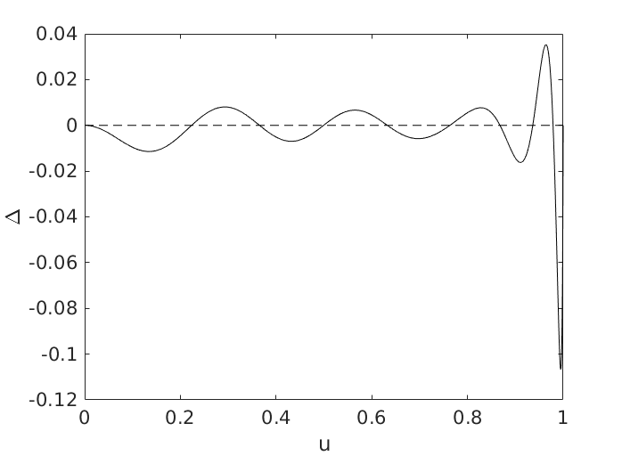
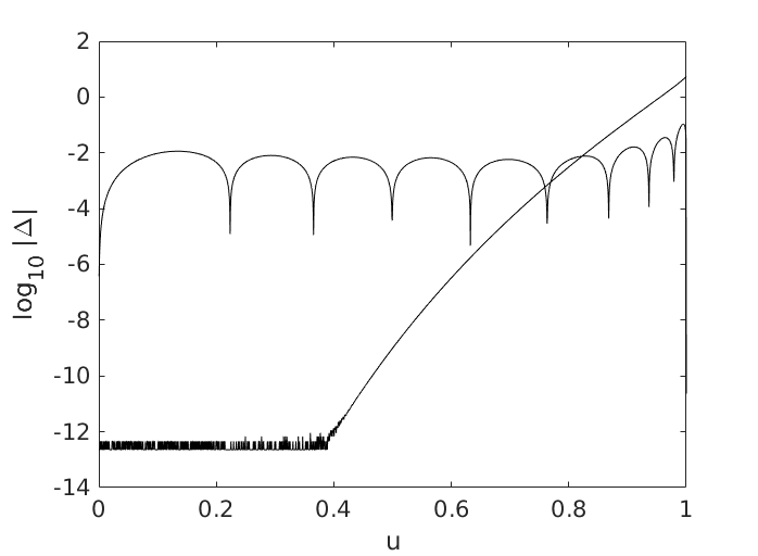
Figure 25: The left panel shows the residual $\Delta(u)$ of the Lane–Emden equation with our polynomial approximation to the solution. The right panel shows the same residuals on a logarithmic scale, compared with the residuals obtained with our truncated Taylor series.

The mass $M(r)$ within radius $r$

If $\rho(r)=\lambda\,(f(u))^{3/2}$ is the mass density at a radius $r=bu$, with $\lambda=\rho_{c}/\alpha^{3/2}$, then the total mass within $r$ is

$$M(r)=4\pi\lambda b^{3}\int_{0}^{u}\mbox{d}v\;v^{2}\,(f(v))^{3/2}=-4\pi\lambda b^{3}\,u^{2}f^{\prime}(u)\;.$$ (126)

We use Eq. (108). Here $f^{\prime}(u)<0$ for $u>0$. The fraction of the total mass within $r=bu$ is

$$F(u)=\frac{u^{2}f^{\prime}(u)}{f^{\prime}(1)}\;.$$ (127)

This is plotted in Fig. 26.

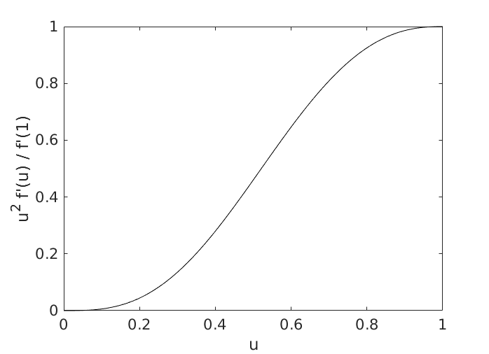
Figure 26: The mass fraction as a function of $u$.

The method for generating one random point from the Lane–Emden density distribution is to generate a random number $w\in{[0,1]}$ and solve the equation $F(u)=w$ for $u$. The radius is $r=bu$, with a scaling factor $b$ to be determined later. The $x,y,z$ coordinates are

$$x=r\sin\vartheta\,\cos\varphi\;,\qquad y=r\sin\vartheta\,\cos\varphi\;,\qquad z=r\cos\vartheta\;.$$ (128)

We generate uniform random variables $w_{1},w_{2}\in{[0,1]}$ and define

$$\cos\vartheta=2w_{1}-1\;,\qquad\sin\vartheta=\sqrt{1-\cos^{2}\vartheta}\;,\qquad\varphi=2\pi w_{2}\;.$$ (129)

We used this Monte Carlo method to generate 10 000 points. For every pair of points we compute their mutual distance $d$. We compute the scaling factor $b$ by minimizing the energy, Eq. (53), or equivalently by requiring the virial theorem to hold, Eq. (54). Repeating the calculation several times, we get a mean value with a statistical error,

$$b=5.2760\pm 0.0080\;.$$ (130)

Since by definition $u\leq 1$, $b$ is the outer radius of the cloud of 10 000 particles. The same Monte Carlo data give a root mean square radius which is

$$r_{m}=2.9220\pm 0.0029\;,$$ (131)

and an average distance between points which is

$$\langle d\rangle=3.8432\pm 0.0037\;.$$ (132)

The average energy per particle pair is

$$\langle E_{2}\rangle=-0.16253\pm 0.00015\;.$$ (133)

Note on numerical methods

We write $f(u)=g(v)$ with $v=u^{2}$. The derivatives of these functions are

$$f^{\prime}(u)=2ug^{\prime}(v)\;,\qquad f^{\prime\prime}(u)=4vg^{\prime\prime}(v)+2g^{\prime}(v)\;.$$ (134)

The following Matlab function computes $f,f^{\prime},f^{\prime\prime}$ and (internally only) $g,g^{\prime},g^{\prime\prime}$. It also computes the residual $\Delta$ of the Lane–Emden equation. The input argument $u$ may be a matrix of any size, then the outputs $f,f^{\prime},f^{\prime\prime},\Delta$ are matrices of the same size. Before calling the function we need to declare the coefficients cf to be global and assign values to them. Note that “$.*$” denotes elementwise multiplication of matrices.

Matlab code for computing the function $f(u)$, its derivatives, and the residue of Eq. (108).

⬇

function [f,f1,f2,Delta] = ff(u)

global cf

v = u.*u;

g = cf(12)+cf(13)*v;

g1 = cf(13);

g2 = 0;

for k=2:12

g2 = 2*g1+g2.*v;

g1 = g+g1.*v;

g = cf(13-k)+g.*v;

end

g = max(g,0);

f = g;

f1 = 2*u.*g1;

f2 = 4*v.*g2+2*g1;

Delta = f2+4*g1+g.^(3/2);

Matlab code for computing the mass fraction $F(u)$, and the inverse of this function.

⬇

function OUT = F(u)

[f1,fd1] = ff(1);

[f,fd] = ff(u);

OUT = u.*u.*fd/fd1;

function OUT = Finv(v)

u1 = 0;

u2 = 1;

u = 10;

ua = 20;

while (u%*$\sim$*)=ua)

ua = u;

u = 0.5*(u1+u2);

if (F(u)<v)

u1 = u;

else

u2 = u;

end

end

OUT = u;

References

-
[1]
Y. Hopstad and J. Myrheim,
Computer simulations of rotating systems of few particles bound by gravitation.
Int. J. Mod. Phys. C 27, 1650142 (2016). -
[2]
S. Chandrasekhar,
An Introduction to the Study of Stellar Structure.
Dover edition (1958). - [3] R. Emden, Gaskuglen. Verlag B.G. Teubner, Leipzig und Berlin (1907).
-
[4]
A.S. Eddington,
The Internal Constitution of the Stars.
Cambridge University Press (1926). -
[5]
E.A. Milne,
The Equilibrium of a Rotating Star.
Monthly Notices of the Royal Astronomical Society 83, 118 (1923). -
[6]
F.L. Espinosa and M. Rieutord,
Gravity Darkening in Rotating Stars.
Astron. Astrophys. 533, A43 (2011). -
[7]
S. Chandrasekhar,
The Equilibrium of Distorted Polytropes.
Monthly Notices of the Royal Astronomical Society 93, 390-405 (1933). -
[8]
J.H. Jeans,
Problems of Cosmogony and Stellar Dynamics.
Cambridge University Press (1919). -
[9]
J.H. Jeans,
Astronomy and Cosmogony.
Cambridge University Press (1929). -
[10]
J.H. Jeans,
Bakerian Lecture 1917: The Configurations of Rotating Compressible Masses.
Philosophical Transactions of the Royal Society of London, Series A. 218, 157-210 (1919). -
[11]
K.V. Kholshevnikov,
On the Lyapunov Theory of Equilibrium Figures
of Celestial Bodies.
Vestnik St. Petersburg University Mathematics 40, 123 (2007). -
[12]
R.A. James,
The Structure and Stability of Rotating Gas Masses.
Astrophys. J. 140, 552 (1964). -
[13]
J.J. Monaghan and I.W. Roxburgh,
The Structure of Rapidly Rotating Polytropes.
Monthly Notices of the Royal Astronomical Society 131, 13-22 (1965). -
[14]
P.H. Roberts,
On Highly Rotating Polytropes. I, II
Astrophys. J. 137, 1129 and 138, 809 (1963). -
[15]
M. Hurley and P.H. Roberts,
On Highly Rotating Polytropes. III
Astrophys. J. 140, 583 (1964). -
[16]
D. Kong, K. Zhang, and G. Schubert,
Self-consistent internal structure of a rotating gaseous planet and its comparison with an approximation by oblate spheroidal equidensity surfaces.
Physics of the Earth and Planetary Interiors 249, 43 (2015). -
[17]
M. Rieutord, F. Espinosa Lara, and B. Putigny,
An algorithm for computing the 2D structure of fast rotating stars.
J. Comput. Phys. 318, 277 (2016). -
[18]
D. Gondek-Rosinska and E. Gourgolhon,
Jacobi-like bar mode instability of relativistic rotating bodies.
Phys. Rev. D 66, 044021 (2002). -
[19]
P.H. Chavanis and M. Rieutord,
Statistical mechanics and phase diagrams of rotating self-gravitating fermions.
Astronomy and Astrophysics 412, 1 (2003). -
[20]
S.L. Shapiro and S.A. Teukolsky,
Black Holes, White Dwarfs, and Neutron Stars. Wiley (1983). - [21] J.-L. Tassoul, Theory of Rotating Stars. Princeton University Press (1978).
-
[22]
I.W. Roxburgh and L.M. Stockman,
Power series solutions of the polytrope equations.
Monthly Notices of the Royal Astronomical Society 303, 466 (1999).