Ensembles of Locally Independent Prediction Models

Abstract

Ensembles depend on diversity for improved performance. Many ensemble training methods, therefore, attempt to optimize for diversity, which they almost always define in terms of differences in training set predictions. In this paper, however, we demonstrate the diversity of predictions on the training set does not necessarily imply diversity under mild covariate shift, which can harm generalization in practical settings. To address this issue, we introduce a new diversity metric and associated method of training ensembles of models that extrapolate differently on local patches of the data manifold. Across a variety of synthetic and real-world tasks, we find that our method improves generalization and diversity in qualitatively novel ways, especially under data limits and covariate shift.

1 Introduction

An ensemble is generally more accurate than its constituent models. However, for this to hold true, those models must make different errors on unseen data (?; ?). This is often described as the ensemble’s “diversity.”

Despite diversity’s well-recognized importance, there is no firm consensus on how best to foster it. Some procedures encourage it implicitly, e.g. by training models with different inputs (?), while others explicitly optimize for proxies (?) that tend to be functions of differences in training set predictions (?; ?).

However, there has been increasing criticism of supervised machine learning for focusing too exclusively on cases where training and testing data are drawn from the same distribution (?). In many real-world settings, this assumption does not hold, e.g. due to natural covariate shift over time (?) or selection bias in data collection (?). Intuitively, we might hope that a “diverse” ensemble would more easily adapt to such problems, since ideally different members would be robust to different shifts. In this paper, however, we find that diverse ensemble methods that only encourage differences in training predictions often perform poorly under mild drift between training and test, in large part because models are not incentivized to make different predictions where there is no data. We also find that ensemble methods that directly optimize for diverse training predictions face inherent tradeoffs between diversity and accuracy and can be very sensitive to hyperparameters.

To resolve these issues, we make two main contributions, specifically (1) a novel and differentiable diversity measure, defined as a formal proxy for the ability of classifiers to extrapolate differently away from data, and (2) a method for training an ensemble of classifiers to be diverse by this measure, which we hypothesize will lead to more robust predictions under distributional shifts with no inherent tradeoffs between diversity and accuracy except those imposed by the dataset. We find this hypothesis holds on a range of synthetic and real-world prediction tasks.

2 Related Work

Ensembling is a well-established subfield of supervised learning (?; ?; ?; ?), and one of its important lessons is that model diversity is a necessary condition for creating predictive and robust ensembles (?). There are a number of methods for fostering diversity, which can be roughly divided into two categories: those that implicitly promote diversity by random modifications to training conditions, and those that explicitly promote it by deliberate modifications to the objective function.

Some implicit diversity methods operate by introducing stochasticity into which models see which parts of the data, e.g. by randomly resampling training examples (?) or subsets of input features (?). Others exploit model parameter stochasticity, e.g. by retraining from different initializations (?) or sampling from parameter snapshots saved during individual training cycles (?).

Methods that explicitly encourage diversity include boosting (?; ?), which sequentially modifies the objective function of each model to specialize on previous models’ mistakes, or methods like negative correlation learning (?) amended cross-entropy (?), and DPPs over non-maximal predictions (?), which simulateously train models with penalities on both individual errors and pairwise similarities. Finally, methods such as Diverse Ensemble Evolution (?) and Competition of Experts (?) use explicit techniques to encourage models to specialize in different regions of input space.

Although at first glance these diverse training techniques seem quite diverse themselves, they are all similar in a crucial respect: they encourage diversity in terms of training set predictions. In the machine learning fairness, adversarial robustness, and explainability communities, however, there has been increasing movement away from the assumption that train is similar to test. For example, many methods for locally explaining ML predictions literally present simplified approximations of how models extrapolate away from given points (?; ?; ?), while adversarial attacks (and defenses) exploit (and mitigate) pathological extrapolation behavior (?; ?), sometimes in an ensemble setting (?). Although our focus is not explicitly on explanability or adversarial robustness, our method can be seen as a reapplication of techniques in those subfields to the problem of ensemble diversity.

Also related is the subfield of streaming data, which sometimes uses ensemble diversity metrics as a criteria for deciding when covariates have shifted sufficiently to warrant retraining (?; ?). Although our focus remains on non-streaming classification, the method we introduce may be applicable to that domain.

3 Method

In this section, building on ? (?), we define our diversity measure and training procedure, beginning with notation. We use $x$ to denote $D$-dimensional inputs, which are supported over an input space $\Omega_{x}\subseteq\mathbb{R}^{D}$. We use $y$ to denote prediction targets in an output space $\Omega_{y}$. In this paper, $\Omega_{y}$ will be $\mathbb{R}$, and we focus on the case where it represents a log-odds used for binary classification, but our method can be generalized to classification or regression in $\mathbb{R}^{K}$ given any notion of distance between outputs. We seek to learn prediction models $f(\cdot;\theta):\Omega_{x}\to\Omega_{y}$ (parameterized by $\theta$) that estimate $y$ from $x$. We assume these models $f$ are differentiable with respect to $x$ and $\theta$ (which is true for linear models and neural networks).

In addition, we suppose a joint distribution over inputs and targets $p(x,y)$ and a distribution $p(y|f(x;\theta))$ quantifying the likelihood of the observed target given the model prediction. Typically, during training, we seek model parameters that maximize the likelihood of the observed data, $\mathbb{E}_{p(x,y)}\left[\log p(y|f(x;\theta))\right]$.

3.1 Diversity Measure: Local Independence

We now introduce a model diversity measure that quantifies how differently two models generalize over small patches of the data manifold $\Omega_{x}$. Formally, we define an $\epsilon$-neighborhood of $x$, denoted $N_{\epsilon}(x)$, on the data manifold to be the intersection of an $\epsilon$-ball centered at $x$ in the input space, $\mathcal{B}_{\epsilon}(x)\subset\mathbb{R}^{D}$, and the data manifold: $N_{\epsilon}(x)=\mathcal{B}_{\epsilon}(x)\cap\Omega$. We capture the notion of generalization difference on a small neighborhood of $x$ through an intuitive geometric condition: we say that two functions $f$ and $g$ generalize maximally differently at $x$ if $f$ is invariant in the direction of of the greatest change in $g$ (or vice versa) within an $\epsilon$-neighborhood around $x$. That is:

$$f\left(x\right)=f\left(x_{g_{\text{max}}}\right),\quad\text{for all }\epsilon^{\prime}<\epsilon,$$ (1)

where we define $x_{g_{\text{max}}}=\displaystyle\operatorname*{arg\,max}_{x^{\prime}\in N_{\epsilon^{\prime}}(x)}g(x^{\prime})$. In other words, perturbing $x$ by small amounts to increase $g$ inside $N_{\epsilon}$ does not change the value of $f$. In the case that a choice of $\epsilon$ exists to satisfy Equation 1, we say that $f$ is locally independent at $x$. We call $f$ and $g$ locally independent without qualification if for every $x\in\Omega_{x}$ the functions $f$ and $g$ are locally independent at $x$ for some choice of $\epsilon$. We note that in order for the right-hand side expression of 1 to be well-defined, we assume that the gradient of $g$ is not zero at $x$ and that $\epsilon$ is chosen to be small enough that $g$ is convex or concave over $N_{\epsilon}(x)$.

In the case that $f$ and $g$ are classifiers, local independence intuitively implies a kind of dissimilarity between their decision boundaries. For example, if $f$ and $g$ are linear and the data manifold is Euclidean, then $f$ and $g$ are locally independent if and only if their decision boundaries are orthogonal.

This definition motivates the formulation of a diversity measure, $\mathtt{IndepErr}(f,g)$, quantifying how far $f$ and $g$ are from being locally independent:

$${\mathtt{IndepErr}(f,g)\equiv\mathbb{E}\left[\left(f\left(x_{g_{\text{max}}}\right)-f\left(x\right)\right)^{2}\right].}$$ (2)

3.2 Local Independence Training (LIT)

Using Equation 2, we can formulate an ensemble-wide loss function $\mathcal{L}$ for a set of models $\{\theta_{m}\}$ as follows, which we call local independence training:

$${\begin{split}\mathcal{L}(\{\theta_{m}\})=&\sum_{m}\mathbb{E}_{p(x,y)}\left[-\log p(y|f(x;\theta_{m}))\right]\\ &+\lambda\sum_{\ell\neq m}\mathtt{IndepErr}(f(\cdot;\theta_{m}),f(\cdot;\theta_{\ell})).\end{split}}$$ (3)

The first term encourages each model $f_{m}$ to be predictive and the second encourages diversity in terms of $\mathtt{IndepErr}$ (with a strength hyperparameter $\lambda$). Computing $\mathtt{IndepErr}$ exactly, however, is challenging, because it requires an inner optimization of $g$. Although it can be closely approximated for fixed small $\epsilon$ with projected gradient descent as in adversarial training (?), that procedure is computationally intensive. If we let $\epsilon\to 0$, however, we can approximate $x_{g_{\text{max}}}$ by a fairly simple equation that only needs to compute $\nabla g$ once per $x$. In particular, we observe that under certain smoothness assumptions on $g$, with unconstrained $\Omega_{x}$, and as $\epsilon\to 0$, we can make the approximation

$$x_{g_{\text{max}}}\approx x+\epsilon\nabla g(x).$$ (4)

Assuming similar smoothness assumptions on $f$ (so we can replace it by its first-order Taylor expansion), we see that

$${\begin{split}f(x_{g_{\text{max}}}&)-f(x)\\ &\approx f(x+\epsilon\nabla g(x))-f(x)\\ &=\left[f(x)+\epsilon\nabla f(x)\cdot\nabla g(x)+\mathcal{O}(\epsilon^{2})\right]-f(x)\\ &\approx\epsilon\nabla f(x)\cdot\nabla g(x).\end{split}}$$ (5)

In other words, the independence error between $f$ and $g$ is approximately equal to the dot product of their gradients $\nabla f(x)\cdot\nabla g(x)$. Empirically, we find it helpful to normalize the dot product and work in terms of cosine similarity $\cos(\nabla f(x),\nabla g(x))\equiv\frac{\nabla f(x)\cdot\nabla g(x)}{||\nabla f(x)||_{2}||\nabla g(x)||_{2}}\in[-1,1]$. We also add a small constant value to the denominator to prevent numerical underflow.

Alternate statistical formulation:

As another way of obtaining this cosine similarity approximation, suppose we sample small perturbations $\boldsymbol{\epsilon}{\sim}\mathcal{N}(0,\sigma^{2}\mathbbm{1})$ and evaluate $f(x+\boldsymbol{\epsilon}){-}f(x)$ and $g(x+\boldsymbol{\epsilon}){-}g(x)$. As $\sigma{\to}0$, these differences approach $\boldsymbol{\epsilon}\cdot\nabla f(x)$ and $\boldsymbol{\epsilon}\cdot\nabla g(x)$, which are 1D Gaussian random variables whose correlation is given by $\cos(\nabla f(x),\nabla g(x))$ and whose mutual information is ${-}\textstyle{\frac{1}{2}}\ln(1-\cos^{2}(\nabla f(x),\nabla g(x)))$ per Section A.3. Therefore, making the input gradients of $f$ and $g$ orthogonal is equivalent to enforcing statistical independence between their outputs when we perturb $x$ with samples from $\mathcal{N}(0,\sigma^{2}\mathbbm{1})$ as $\sigma\to 0$. This could be used as an alternate definition of “local independence.”

Final LIT objective term:

Motivated by the approximations and discussion above, we substitute

$${\begin{split}\mathtt{CosIndepErr}(f,g)\equiv\mathbb{E}\left[\cos^{2}(\nabla f(x),\nabla g(x))\right]\\ \end{split}}$$ (6)

into our ensemble loss from Equation (3), which gives us a final loss function

$${\begin{split}\mathcal{L}(\{\theta_{m}\})=&\sum_{m}\mathbb{E}_{p(x,y)}\left[-\log p(y|f(x;\theta_{m}))\right]\\ &+\lambda\sum_{\ell\neq m}\mathbb{E}_{p(x)}\left[\cos^{2}(\nabla f(x;\theta_{m}),\nabla f(x;\theta_{\ell}))\right].\end{split}}$$ (7)

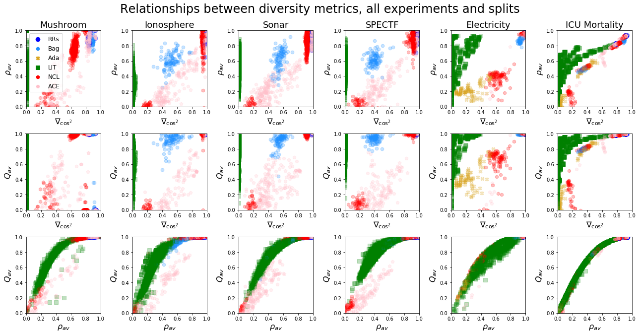
Note that we will sometimes abbreviate $\mathtt{CosIndepErr}$ as $\nabla_{\cos^{2}}$. In Section 4 as well as Figure 10, we show that $\mathtt{CosIndepErr}$ is meaningfully correlated with other diversity measures and therefore may be useful in its own right, independently of its use within a loss function.

4 Experiments

On synthetic data, we show that ensembles trained with LIT exhibit more diversity in extrapolation behavior. On a range of benchmark datasets, we show that the extrapolation diversity in LIT ensembles corresponds to improved predictive performance on test data that are distributed differently than train data. Finally, in a medical data case study, we show that models in LIT ensembles correspond to qualitatively different and clinically meaningful explanations of the data.

Training:

For the experiments that follow, we use 256-unit single hidden layer fully connected neural networks with rectifier activations, trained in Tensorflow with Adam. For the real-data experiments, we use dropout and L2 weight decay with a penalty of 0.0001. Code to replicate all experiments is available at https://github.com/dtak/lit.

Baselines:

We test local independence training (“LIT”) against random restarts (“RRs”), bagging (?) (“Bag”), AdaBoost (?) (“Ada”), 0-1 squared loss negative correlation learning ? (?) (“NCL”), and amended cross-entropy (?) (“ACE”). We omit ? (?) and ? (?) which require more complex inner submodular or adversarial optimization steps, but note that because they also operationalize diversity as making different errors on training points, we expect the results to be qualitatively similar to ACE and NCL.

Hyperparameters:

For our non-synthetic results, we test all methods with ensemble sizes in $\{2,3,5,8,13\}$, and all methods with regularization parameters $\lambda$ (LIT, ACE, and NCL) with 16 logarithmically spaced values between $10^{-4}$ and $10^{1}$, using validation AUC to select the best performing model (except when examining how results vary with $\lambda$ or size). For each hyperparameter setting and method, we run 10 full random restarts (though within each restart, different methods are tested against the same split), and present mean results with standard deviation errorbars.

4.1 Conceptual Demonstration

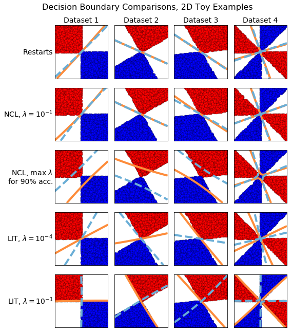
To provide an initial demonstration of our method and the limitations of training set prediction diversity, we present several sets of 2D synthetic examples in Figure 1. These 2D examples are constructed to have data distributions that satisfy our assumption that $N_{\epsilon}(x)\approx\mathcal{B}_{\epsilon}(x)$ locally around almost all of the points, but nevertheless contain significant gaps. These gaps result in the possibility of learning multiple classifiers that have perfect accuracy on the training set but behave differently when extrapolating. Indeed, in all of these examples, if we have just two classifiers, they can completely agree on training and completely disagree in the extrapolation regions.

Figure 1: 2D synthetic datasets with gaps. We argue that “diverse” ensemble methods applied to these datasets should produce accurate models with different decision boundaries.

Figure 2: Comparison of local independence training, random restarts and NCL on toy 2D datasets. For each ensemble, the first model’s decision boundary is plotted in orange and the other in dashed blue. Both NCL and LIT are capable of producing variation, but in qualitatively different ways.

Random Split

Method

Mushroom

Ionosphere

Sonar

SPECTF

Electricity

AUC

$\rho_{av}$

$\nabla_{\cos^{2}}$

AUC

$\rho_{av}$

$\nabla_{\cos^{2}}$

AUC

$\rho_{av}$

$\nabla_{\cos^{2}}$

AUC

$\rho_{av}$

$\nabla_{\cos^{2}}$

AUC

$\rho_{av}$

$\nabla_{\cos^{2}}$

RRs

1.0

$\text{1}{\pm}\text{.1}$

$\text{.9}{\pm}\text{0}$

$\text{.95}{\pm}\text{.03}$

$\text{.9}{\pm}\text{.1}$

$\text{1}{\pm}\text{0}$

$\text{.91}{\pm}\text{.06}$

$\text{.9}{\pm}\text{.1}$

$\text{1}{\pm}\text{0}$

$\textbf{.80}{\pm}\text{.06}$

$\text{.9}{\pm}\text{.1}$

$\text{1}{\pm}\text{0}$

$\text{.87}{\pm}\text{.00}$

$\text{1}{\pm}\text{0}$

$\text{1}{\pm}\text{0}$

Bag

1.0

$\text{1}{\pm}\text{0}$

$\text{.9}{\pm}\text{0}$

$\text{.96}{\pm}\text{.02}$

$\text{.7}{\pm}\text{.1}$

$\text{.5}{\pm}\text{.1}$

$\text{.90}{\pm}\text{.06}$

$\text{.5}{\pm}\text{.2}$

$\text{.5}{\pm}\text{.1}$

$\textbf{.80}{\pm}\text{.05}$

$\text{.6}{\pm}\text{.1}$

$\text{.4}{\pm}\text{.1}$

$\text{.87}{\pm}\text{.00}$

$\text{.9}{\pm}\text{0}$

$\text{1}{\pm}\text{0}$

Ada

1.0

—

—

$\text{.95}{\pm}\text{.03}$

—

—

$\text{.91}{\pm}\text{.06}$

—

—

$\textbf{.80}{\pm}\text{.06}$

—

—

$\textbf{.88}{\pm}\text{.00}$

$\text{.2}{\pm}\text{0}$

$\text{.2}{\pm}\text{.1}$

NCL

1.0

$\text{1}{\pm}\text{0}$

$\text{.8}{\pm}\text{0}$

$\text{.96}{\pm}\text{.04}$

$\text{.6}{\pm}\text{.5}$

$\text{.7}{\pm}\text{.3}$

$\textbf{.91}{\pm}\text{.06}$

$\text{.6}{\pm}\text{.5}$

$\text{.7}{\pm}\text{.4}$

$\textbf{.80}{\pm}\text{.07}$

$\text{.6}{\pm}\text{.5}$

$\text{.7}{\pm}\text{.3}$

$\text{.87}{\pm}\text{.00}$

$\text{.4}{\pm}\text{.1}$

$\text{.6}{\pm}\text{0}$

ACE

1.0

$\text{1}{\pm}\text{0}$

$\text{.9}{\pm}\text{0}$

$\text{.94}{\pm}\text{.04}$

$\text{.8}{\pm}\text{.3}$

$\text{.9}{\pm}\text{.2}$

$\text{.90}{\pm}\text{.06}$

$\text{.9}{\pm}\text{.2}$

$\text{1}{\pm}\text{.1}$

$\textbf{.79}{\pm}\text{.06}$

$\text{.8}{\pm}\text{.4}$

$\text{.9}{\pm}\text{.2}$

$\text{.87}{\pm}\text{.00}$

$\text{.9}{\pm}\text{0}$

$\text{1}{\pm}\text{0}$

LIT

1.0

$\text{.9}{\pm}\text{.1}$

$\text{0}{\pm}\text{0}$

$\textbf{.98}{\pm}\text{.01}$

$\text{.3}{\pm}\text{.1}$

$\text{0}{\pm}\text{0}$

$\textbf{.92}{\pm}\text{.05}$

$\text{.5}{\pm}\text{.2}$

$\text{0}{\pm}\text{0}$

$\textbf{.81}{\pm}\text{.06}$

$\text{.4}{\pm}\text{.1}$

$\text{0}{\pm}\text{0}$

$\text{.87}{\pm}\text{.00}$

$\text{.9}{\pm}\text{0}$

$\text{.3}{\pm}\text{.1}$

Extrapolation Split

Method

Mushroom

Ionosphere

Sonar

SPECTF

Electricity

AUC

$\rho_{av}$

$\nabla_{\cos^{2}}$

AUC

$\rho_{av}$

$\nabla_{\cos^{2}}$

AUC

$\rho_{av}$

$\nabla_{\cos^{2}}$

AUC

$\rho_{av}$

$\nabla_{\cos^{2}}$

AUC

$\rho_{av}$

$\nabla_{\cos^{2}}$

RRs

$\text{.92}{\pm}\text{.00}$

$\text{.9}{\pm}\text{0}$

$\text{.8}{\pm}\text{0}$

$\text{.87}{\pm}\text{.02}$

$\text{1}{\pm}\text{0}$

$\text{1}{\pm}\text{0}$

$\text{.81}{\pm}\text{.02}$

$\text{1}{\pm}\text{0}$

$\text{1}{\pm}\text{0}$

$\textbf{.83}{\pm}\text{.05}$

$\text{1}{\pm}\text{0}$

$\text{1}{\pm}\text{0}$

$\text{.86}{\pm}\text{.00}$

$\text{1}{\pm}\text{0}$

$\text{1}{\pm}\text{0}$

Bag

$\text{.91}{\pm}\text{.00}$

$\text{.9}{\pm}\text{0}$

$\text{.9}{\pm}\text{0}$

$\text{.89}{\pm}\text{.04}$

$\text{.6}{\pm}\text{.1}$

$\text{.5}{\pm}\text{.1}$

$\textbf{.82}{\pm}\text{.03}$

$\text{.7}{\pm}\text{.1}$

$\text{.6}{\pm}\text{0}$

$\textbf{.83}{\pm}\text{.05}$

$\text{.6}{\pm}\text{.1}$

$\text{.4}{\pm}\text{0}$

$\text{.86}{\pm}\text{.00}$

$\text{.9}{\pm}\text{0}$

$\text{.9}{\pm}\text{0}$

Ada

$\text{.92}{\pm}\text{.01}$

—

—

$\text{.87}{\pm}\text{.02}$

—

—

$\text{.81}{\pm}\text{.03}$

—

—

$\textbf{.83}{\pm}\text{.05}$

—

—

$\text{.86}{\pm}\text{.00}$

$\text{.3}{\pm}\text{.1}$

$\text{.3}{\pm}\text{.2}$

NCL

$\text{.94}{\pm}\text{.01}$

$\text{.6}{\pm}\text{.2}$

$\text{.6}{\pm}\text{.1}$

$\text{.90}{\pm}\text{.02}$

$\text{.8}{\pm}\text{.3}$

$\text{.9}{\pm}\text{.2}$

$\text{.78}{\pm}\text{.06}$

$\text{.5}{\pm}\text{.5}$

$\text{.6}{\pm}\text{.3}$

$\text{.81}{\pm}\text{.12}$

$\text{.5}{\pm}\text{.6}$

$\text{.7}{\pm}\text{.3}$

$\text{.86}{\pm}\text{.00}$

$\text{.9}{\pm}\text{.2}$

$\text{1}{\pm}\text{.1}$

ACE

$\text{.92}{\pm}\text{.00}$

$\text{.9}{\pm}\text{0}$

$\text{.8}{\pm}\text{0}$

$\text{.90}{\pm}\text{.03}$

$\text{.3}{\pm}\text{.4}$

$\text{.5}{\pm}\text{.3}$

$\text{.77}{\pm}\text{.06}$

$\text{.6}{\pm}\text{.5}$

$\text{.7}{\pm}\text{.3}$

$\text{.72}{\pm}\text{.16}$

$\text{.5}{\pm}\text{.6}$

$\text{.7}{\pm}\text{.4}$

$\text{.86}{\pm}\text{.00}$

$\text{1}{\pm}\text{0}$

$\text{1}{\pm}\text{0}$

LIT

$\textbf{.96}{\pm}\text{.01}$

$\text{.3}{\pm}\text{.1}$

$\text{0}{\pm}\text{0}$

$\textbf{.96}{\pm}\text{.02}$

$\text{.2}{\pm}\text{.1}$

$\text{0}{\pm}\text{0}$

$\textbf{.81}{\pm}\text{.03}$

$\text{.5}{\pm}\text{.1}$

$\text{0}{\pm}\text{0}$

$\textbf{.84}{\pm}\text{.05}$

$\text{.4}{\pm}\text{.1}$

$\text{0}{\pm}\text{0}$

$\textbf{.87}{\pm}\text{.00}$

$\text{.4}{\pm}\text{.2}$

$\text{0}{\pm}\text{0}$

Table 1: Benchmark classification results in both the normal prediction task (top) and the extrapolation task (bottom) over 10 reruns, with errorbars based on standard deviations and bolding based on standard error overlap. On random splits, LIT offers modest AUC improvements over random restarts, on par with other ensemble methods. On extrapolation splits, however, LIT tends to achieve higher AUC. In both cases, LIT almost always exhibits low pairwise Pearson correlation between heldout model errors ($\rho_{av}$), and for other methods, $\rho_{av}$ roughly matches pairwise gradient cosine similarity ($\nabla_{\cos^{2}}$).

In Figure 2, we compare the neural network decision boundaries learned by random restarts, local independence training, and negative correlation learning (NCL) on these examples (we use NCL as a state-of-the-art example of an approach that defines diversity with respect to training predictions). Starting with the top and bottom two rows (random restarts and LIT), we find that random restarts give us essentially identical models, whereas LIT outputs models with meaningfully different decision boundaries even at values of $\lambda$ that are very low compared to its prediction loss term. This is in large part because on most of these tasks (except Dataset 3), there is very little tradeoff to learning a near-orthogonal boundary. At larger $\lambda$, LIT outputs decision boundaries that are completely orthogonal (at the cost of a slight accuracy reduction on Dataset 3).

NCL had more complicated behavior, in large part because of its built-in tradeoff between accuracy and diversity. At low values of $\lambda$ (second from top), we found that NCL produced models with identical decision boundaries, suggesting that training ignored the diversity term. At $\lambda\geq 2$, the predictive performance of one model fell to random guessing, suggesting that training ignored the accuracy term. So in order to obtain meaningfully diverse but accurate NCL models, we iteratively searched for the highest value of $\lambda$ at which NCL would still return two models at least 90% accurate on the training set (by exponentially shrinking a window between $\lambda=1$ and $\lambda=2$ for 10 iterations). What we found (middle row) is that NCL learned to translate its decision boundaries within the support of the training data (incurring an initially modest accuracy cost due to the geometry of the problem) but not modify them outside the training support. Although this kind of diversity is not necessarily bad (since the ensemble accuracy remains perfect), it is qualitatively different from the kind of diversity encouraged by LIT—and only emerges at carefully chosen hyperparameter values. The main takeaway from this set of synthetic examples is that methods that encourage diverse extrapolation (like LIT) can produce significantly different ensembles than methods that encourage diverse prediction (like NCL).

4.2 Classification Benchmarks

Next, we test our method on several standard binary classification datasets from the UCI and MOA repositories (?; ?). These are mushroom, ionosphere, sonar, spectf, and electricity (with categorical features one-hot encoded, and all features z-scored). For all datasets, we randomly select 80% of the dataset for training and 20% for test, then take an additional 20% split of the training set to use for validation. In addition to random splits, we also introduce an extrapolation task, where instead of splitting datasets randomly, we train on the 50% of points closest to the origin (i.e. where $||x||_{2}$ is less than its median value) and validate/test on the remaining points (which are furthest from the origin). This test is meant to evaluate robustness to covariate shift.

For each ensemble, we measure heldout AUC and accuracy, our diversity metric CosIndepErr (abbreviated as $\nabla_{\cos^{2}}$), and several classic diversity metrics ($\rho_{av}$, $Q_{av}$, and $\kappa$) defined by ? (?). Table 1 compares heldout AUC, $\rho_{av}$, and $\nabla_{\cos^{2}}$ after cross-validating $\lambda$ and the ensemble size. More complete enumerations of AUC, accuracy, and diversity metrics are shown in Figures 9 and 10. In general, we find that LIT is competitive on random splits, strongest on extrapolation, and significantly improves heldout prediction diversity across the board. We also find that $\nabla_{\cos^{2}}$ is meaningfully related to other diversity metrics for all models that do not optimize for it.

4.3 ICU Mortality Case Study

As a final set of experiments, we run a more in-depth case study on a real world clinical application. In particular, we predict in-hospital mortality for a cohort of $n=1,053,490$ patient visits extracted from the MIMIC-III database (?) based on on labs, vital signs, and basic demographics. We follow the same cohort selection and feature selection process as ? (?). In addition to this full cohort, we also test on a limited data task where we restrict the size of the training set to $n=1000$ to measure robustness.

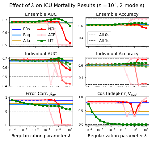
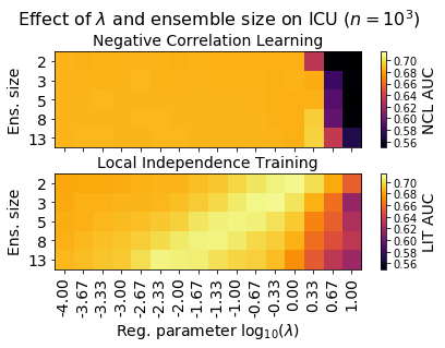
We visualize the results of these experiments in several ways to help tease out the effects of $\lambda$, ensemble size, and dataset size on individual and ensemble predictive performance, diversity, and model explanations. Table 2 shows overall performance and diversity metrics for these two tasks after cross-validation, along with the most common values of $\lambda$ and ensemble size selected for each method. Drilling into the $n=1000$ results, Figure 3 visualizes how multiple metrics for performance (AUC and accuracy) and diversity ($\rho_{av}$ and $\nabla_{\cos^{2}}$) change with $\lambda$, while Figure 4 visualizes the relationship between optimal $\lambda$ and ensemble size.

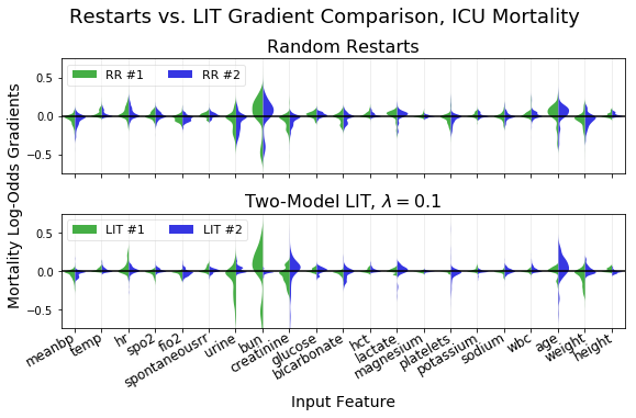
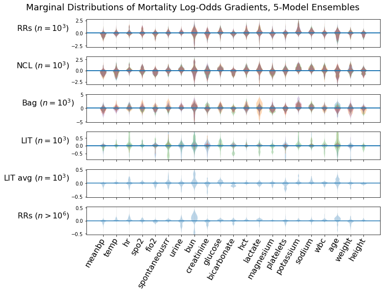
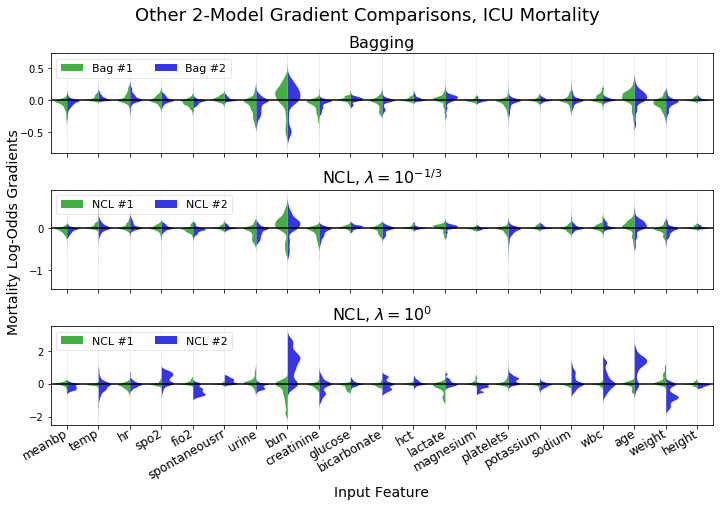
Figure 5 (as well as Figures 7 and 8) visualize changes in the marginal distributions of input gradients for each model in their explanatory sense (?). As a qualitative evaluation, we discussed these explanation differences with two intensive care unit clinicians and found that LIT revealed meaningful redundancies in which combinations of features encoded different underlying conditions.

ICU Mortality Task, Full Dataset ($n>10^{6}$)
Method	AUC	$\rho_{av}$	$\nabla_{\cos^{2}}$	#	$\lambda$
RRs	$\text{.750}{\pm}\text{.000}$	$\text{.9}{\pm}\text{0}$	$\text{.9}{\pm}\text{0}$	13	—
Bag	$\text{.751}{\pm}\text{.000}$	$\text{.9}{\pm}\text{0}$	$\text{.9}{\pm}\text{0}$	8	—
Ada	$\textbf{.752}{\pm}\text{.003}$	$\text{0}{\pm}\text{0}$	$\text{0}{\pm}\text{0}$	8	—
ACE	$\text{.750}{\pm}\text{.000}$	$\text{.9}{\pm}\text{0}$	$\text{.9}{\pm}\text{0}$	13	$10^{0.33}$
NCL	$\textbf{.753}{\pm}\text{.001}$	$\text{.3}{\pm}\text{.2}$	$\text{.2}{\pm}\text{.2}$	13	$10^{0.00}$
LIT	$\text{.750}{\pm}\text{.001}$	$\text{.8}{\pm}\text{0}$	$\text{.3}{\pm}\text{0}$	3	$10^{-4.00}$
ICU Mortality Task, Limited Slice ($n=10^{3}$)
Method	AUC	$\rho_{av}$	$\nabla_{\cos^{2}}$	#	$\lambda$
RRs	$\text{.684}{\pm}\text{.001}$	$\text{.8}{\pm}\text{0}$	$\text{.8}{\pm}\text{0}$	8	—
Bag	$\text{.690}{\pm}\text{.002}$	$\text{.5}{\pm}\text{0}$	$\text{.3}{\pm}\text{0}$	8	—
Ada	$\text{.678}{\pm}\text{.003}$	$\text{.6}{\pm}\text{0}$	$\text{.5}{\pm}\text{0}$	2	—
ACE	$\text{.684}{\pm}\text{.001}$	$\text{.8}{\pm}\text{0}$	$\text{.8}{\pm}\text{0}$	2	$10^{-2.67}$
NCL	$\text{.697}{\pm}\text{.006}$	$\text{.2}{\pm}\text{.4}$	$\text{.6}{\pm}\text{.2}$	13	$10^{0.33}$
LIT	$\textbf{.711}{\pm}\text{.001}$	$\text{.1}{\pm}\text{0}$	$\text{0}{\pm}\text{0}$	13	$10^{-2.33}$

Table 2: Quantitative results on the ICU mortality prediction task, where $\#$ and $\lambda$ signify the most commonly selected values of ensemble size and regularization parameter chosen for each method. On the full data task, although all methods perform similarly, NCL and AdaBoost edge out slightly, and LIT consistently selects its weakest regularization parameter. On the limited data task, LIT significantly outperforms baselines, with NCL and Bagging in second, ACE indistinguishable from restarts, and significantly worse performance for AdaBoost (which overfits).

Figure 3: Changes in individual AUC/accuracy and ensemble diversity with $\lambda$ for two-model ensembles on the ICU mortality dataset (averaged across 10 reruns, error-bars omitted for clarity). For NCL and ACE, there is a wide low-$\lambda$ regime where they are indistinguishable from random restarts. This is followed by a very brief window of meaningful diversity (around $\lambda=1$ for NCL, slightly lower for ACE), after which both methods output pairs of models which always predict 0 and 1 (respectively), as shown by the error correlation dropping to -1. LIT, on the other hand, exhibits smooth drops in individual model predictive performance, with error correlation falling towards 0. Results for other ensemble sizes were qualitatively similar.

Figure 4: Another exploration of the effect of ensemble size and $\lambda$ on ICU mortality predictions. In particular, we find that for LIT on this dataset, the optimal value of $\lambda$ depends on the ensemble size in a roughly log-linear relationship. Because $D$-dimensional datasets can support a maximum of $D$ locally independent models (and only one model if the data completely determines the decision boundary), it is intuitive that there should be an optimal value. For NCL, we also observe an optimal value near $10^{0.33}$, but with a less clear relationship to ensemble size and very steep dropoff to random guessing at slightly higher $\lambda$.

Figure 5: Differences in cross-patient gradient distributions of ICU mortality prediction models for random restart and locally independent ensembles (similar plots for other methods are shown in Figure 8). Features with mass consistently above the x-axis have positive associations with predicted mortality (increasing them increases predicted mortality) while those with mass consistently below the x-axis have negative associations (decreasing them increases predicted mortality). Distance from the x-axis corresponds to the association strength. Models trained normally (top) consistently learn positive associations with age and bun (blood urea nitrogen; larger values indicate kidney failure) and negative associations with weight and urine (low weight is correlated with mortality; low urine output also indicates kidney failure or internal bleeding). However, they also learn somewhat negative associations with creatinine, which confused clinicians because high values are another indicator of kidney failure. When we trained LIT models, however, we found that creatinine regained its positive association with mortality (in model 2), while the other main features were more or less divided up. This collinearity between creatinine and bun/urine in indicating organ problems (and revealed by LIT) was one of the main insights derived in our qualitative evaluation with ICU clinicians.

5 Discussion

LIT matches or outperforms other methods, especially under data limits or covariate shift.

On the UCI datasets under $\text{train}\overset{d}{\approx}\text{test}$ conditions (random splits), LIT always offers at least modest improvements over random restarts, and often outperforms other baselines. Under extrapolation splits, LIT tends to do significantly better. This pattern repeats itself on the normal vs. data-limited versions of ICU mortality prediction task. We hypothesize that on small or selectively restricted datasets, there is typically more predictive ambiguity, which hurts the generalization of normally trained ensembles (who consistently make similar guesses on unseen data). LIT is more robust to these issues.

Gradient cosine similarity can be a meaningful diversity metric.

In Table 1 as well as our more complete results in Figure 10, we saw that for non-LIT methods, gradient similarity $\nabla_{\cos^{2}}$ (which does not require labels to compute) was often similar in value to error correlation $\rho_{av}$ (as well as the interrater agreement $\kappa$, or Yule’s Q-statistic $Q_{av}$ after a monotonic transformation—all measures which do require labels to compute). One potential explanation for this correspondence is that, by our analysis at the end of Section 3.2, $\nabla_{\cos^{2}}$ can literally be interpreted as an average squared correlation (between changes in model predictions over infinitesimal Gaussian perturbations away from each input). We hypothesize that $\nabla_{\cos^{2}}$ may be a useful quantity independently of LIT.

LIT is less sensitive to hyperparameters than baselines, but ensemble size matters more.

In both our synthetic examples (Figure 2) and our ICU mortality results (Figures 3 and 4), we found that LIT produced qualitatively similar (diverse) results over several orders of magnitude of $\lambda$. NCL, on the other hand, required careful tuning of $\lambda$ to achieve meaningful diversity (before its performance plummeted). In line with the results from our synthetic examples, we believe this difference stems from the fact that NCL’s diversity term is formulated as a direct tradeoff with individual model accuracy, so the balance must be precise, whereas LIT’s diversity term can theoretically be completely independent of individual model accuracy (which is true by construction in the synthetic examples). However, datasets only have the capacity to support a limited number of (mostly or completely) locally independent models. On the synthetic datasets, this capacity was exactly 2, but on real data, it is generally unknown, and it may be possible to achieve similar results either with a small fully independent ensemble or a large partially independent ensemble. For example, in Figure 4, we show that we can achieve similar improvements to ICU mortality prediction with 2 highly independent ($\lambda=10^{0}$) models or 13 more weakly independent ($\lambda=10^{-2.33}$) models. We hypothesize that the trend-line of optimal LIT ensemble size and $\lambda$ may be a useful tool for characterizing the amount of ambiguity present in a dataset.

Interpretation of individual LIT models can yield useful dataset insights.

In Figure 5, we found that in discussions with ICU clinicians, mortality feature assocations for normally trained neural networks were somewhat confusing due to hidden collinearities. LIT models made more clinical sense individually, and the differences between them helped reveal those collinearities (in particular between elevated levels of blood urea nitrogen and creatinine). Because LIT ensembles are often optimal when small, and because individual LIT models are not required to sacrifice accuracy for diversity, they may enable different and more useful kinds of data interpretation than other ensemble methods.

Limitations.

LIT does come with restrictions and limitations. In particular, we found that it works well for rectifier activations (e.g. ReLU and softplus) but leads to inconsistent behavior with others (e.g. sigmoid and tanh). This may be related to the linear rather than saturating extrapolation behavior of rectifiers. Because it relies on cosine similarity, LIT is also sensitive to relative changes in feature scaling; however, in practice this issue can be resolved by standardizing variables first.

Additionally, our cosine similarity approximation in LIT makes the assumption that the data manifold is locally similar to $\mathbb{R}^{D}$ near most inputs. However, we introduce generalizations in Section A.1 to handle situations where this is not approximately true (such as with image data).

Finally, LIT requires computing a second derivative (the derivative of the penalty) during the optimization process, which increases memory usage and training time; in practice, LIT took approximately 1.5x as long as random restarts, while NCL took approximately half the time. However, significant progress is being made on making higher-order autodifferentiation more efficient (?), so we can expect improvements. Also, in cases where LIT achieves high accuracy with a comparatively small ensemble size (e.g. ICU mortality prediction), overall training time can remain short if cross-validation terminates early.

6 Conclusion and Future Work

In this paper, we presented a novel diversity metric that formalizes the notion of difference in local extrapolations. Based on this metric we defined an ensemble method, local independence training, for building ensembles of highly predictive base models that generalize differently outside the training set. On datasets we knew supported multiple diverse decision boundaries, we demonstrated our method’s ability to recover them. On real-world datasets with unknown levels of redundancy, we demonstrated that LIT ensembles perform competitively on traditional prediction tasks and were more robust to data scarcity and covariate shift (as measured by training on inliers and testing on outliers). Finally, in our case study on a clinical prediction task in the intensive care unit, we provided evidence that the extrapolation diversity exhibited by LIT ensembles improved data robustness and helped us reach meaningful clinical insights in conversations with clinicians. Together, these results suggest that extrapolation diversity may be an important quantity for ensemble algorithms to measure and optimize.

There are ample directions for future improvements. For example, it would be useful to consider methods for aggregating predictions of LIT ensembles using a more complex mechanism, such as a mixture-of-experts model. Along similar lines, combining pairwise $\mathtt{IndepErr}$s in more informed way, such as a determinantal point process penalty (?) over the matrix of model similarities, may help us better quantify the diversity of the ensemble. Another interesting extension of our work would be to prediction tasks in semi-supervised settings, since labels are generally not required for computing local independence error. Finally, as we observe in the Section 5, some datasets seem to support a particular number of locally independent models. It is worth exploring how to connect this property to attempts to formally quantify and characterize the complexity or ambiguity present in a prediction task (?; ?).

Appendix A Appendix

A.1 Imposing Penalties over Manifolds

In the beginning of our derivation of $\mathtt{CosIndepErr}$ (Equation 4), we assumed that locally, $N_{\epsilon}(x)\approx\mathcal{B}_{\epsilon}(x)$. However, in many cases, our data manifold $\Omega_{x}$ is much lower dimensional than $\mathbb{R}^{D}$. In these cases, we have additional degrees of freedom to learn decision boundaries that, while locally orthogonal, are functionally equivalent over the dimensions which matter. To restrict spurious similarity, we can project our gradients down to the data manifold. Given a local basis for its tangent space, we can accomplish this by taking dot products between $\nabla f$ and $\nabla g$ and each tangent vector, and then use these two vectors of dot products to compute the cosine similarity in Equation 6. More formally, if $J(x)$ is the Jacobian matrix of manifold tangents at $x$, we can replace our regular cosine penalty with

$$\begin{split}\mathtt{ManifIndepErr}(f,g)&\equiv\mathbb{E}\left[\cos^{2}(\nabla f\|_{J}(x),\nabla g\|_{J}(x)),\right]\\ \text{where}\quad&\nabla f\|_{J}(x)=\nabla f(x)^{\intercal}J(x),\\ &\nabla g\|_{J}(x)=\nabla g(x)^{\intercal}J(x)\end{split}$$ (8)

An example of this method applied to a toy example is given in Figure 6. Alternatively, if we are using projected gradient descent adversarial training to minimize the original formulation in Equation 2, we can modify its inner optimization procedure to project input gradient updates back to the manifold.

Figure 6: Synthetic 2D manifold dataset (randomly sampled from a neural network) embedded in $\mathbb{R}^{3}$, with decision boundaries shown in 2D chart space (top) and the 3D embedded manifold space (bottom). Naively imposing LIT penalties in $\mathbb{R}^{3}$ (middle) leads to only slight differences in the chart space decision boundary, but given knowledge of the manifold’s tangent vectors (right), we can recover maximally different chart space boundaries.

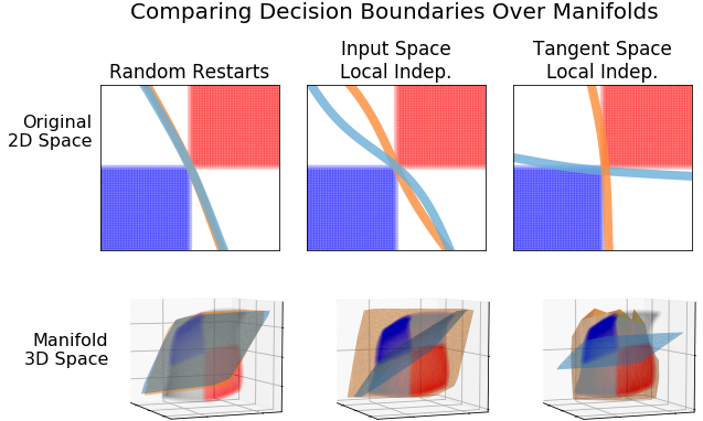
For many problems of interest, we do not have a closed form expression for the data manifold or its tangent vectors. In this case, however, we can approximate one, e.g. by performing PCA or training an autoencoder. Local independence training can also simply be used on top of this learned representation directly.

A.2 Additional Figures

Figure 7: Violin plots showing marginal distributions of ICU mortality input gradients across heldout data for 5-model ensembles trained on the $n=1000$ slice (top 5 plots) and restarts on the full dataset (bottom). Distributions for each model in each ensemble are overlaid with transparency in the top 4 plots. From the top, we see that restarts and NCL learn models with similar gradient distributions. Bagging is slightly more varied, but only LIT (which performs significantly better on the prediction task) exhibits significant differences between models. When LIT gradients on this limited data task are averaged (second from bottom), their distribution comes to resemble (in both shape and scale) that of a model trained on the full dataset (bottom), which may explain LIT’s stronger performance.

Figure 8: Companion to Figure 5 showing differences in the distributions of input gradients for other 2-model ensemble methods. Bagging is largely identical to random restarts, while NCL exhibits a sharp transition with $\lambda$.

Figure 9: Full ensemble AUC and accuracy results by method and ensemble size. LIT usually beats baselines when train $\neq$ test, but the optimal ensemble size (cross-validated in the result tables in the main paper, but expanded here) can vary.

Figure 10: Empirical relationship between our similarity metric (or penalty) $\nabla_{\cos^{2}}$ and more classic measures of prediction similarity such as error correlation ($\rho_{av}$) and the Q-statistic ($Q_{av}$), with one marker for every method, $\lambda$, dataset, split, ensemble size, and restart. In general, we find meaningful relationships between $\nabla_{\cos^{2}}$ and classic diversity metrics, despite the fact that $\nabla_{\cos^{2}}$ does not require ground-truth labels. The bottom row of this figure also shows that LIT models (green) tend to have lower and more widely varying $Q_{av}$ and $\rho_{av}$, indicating greater ability to control heldout prediction diversity through training $\lambda$. We also measured the interrater agreement $\kappa$ but we found the results almost identical to $\rho_{av}$ and omit them to save space.

A.3 Orthogonality and Independence

Here we briefly explain the alternate statistical formulation of local independence given in Section 3.2. Let $x\in\mathbb{R}^{D}$ be a data point, let $f_{1}$ and $f_{2}$ be functions from $\mathbb{R}^{D}\to\mathbb{R}$, and let $\boldsymbol{\epsilon}\sim\mathcal{N}(0,\sigma^{2}\mathbbm{1})$ be a small perturbation. Taylor expanding $f_{1}$ and $f_{2}$ around $x$ and assuming all gradients are nonzero at $x$, we have that

$$\begin{split}f_{i}(x+\boldsymbol{\epsilon})&\approx f_{i}(x)+\nabla f_{i}(x)\cdot\boldsymbol{\epsilon}+\mathcal{O}(\boldsymbol{\epsilon}\cdot\boldsymbol{\epsilon})\\ \end{split}$$

Defining the changes in each $f_{i}$ under the perturbation of $x$ to be $\Delta f_{i}(x)$, and assuming that all gradients are nonzero at $x$ and that we select $\sigma^{2}$ to be small enough that $||\boldsymbol{\epsilon}||^{2}\ll||\boldsymbol{\epsilon}||$ with high probability, we have

$$\Delta f_{i}(x)\equiv f_{i}(x+\boldsymbol{\epsilon})-f_{i}(x)\approx\nabla f_{i}(x)\cdot\boldsymbol{\epsilon}$$

If we now consider $\mathrm{Cov}(\Delta f_{1}(x),\Delta f_{2}(x))$, the covariance of the changes in each function (which we term the “local covariance” between $f_{1}$ and $f_{2}$ at $x$), we see that

$$\begin{split}\mathrm{Cov}&(\Delta f_{1}(x),\Delta f_{2}(x))\\ &\approx\mathbb{E}[(\nabla f_{1}(x)\cdot\boldsymbol{\epsilon}-\mathbb{E}[\nabla f_{1}(x)\cdot\boldsymbol{\epsilon}])\\ &\hskip 22.76228pt(\nabla f_{2}(x)\cdot\boldsymbol{\epsilon}-\mathbb{E}[\nabla f_{2}(x)\cdot\boldsymbol{\epsilon}])]\\ &=\mathbb{E}[(\nabla f_{1}(x)\cdot\boldsymbol{\epsilon})(\nabla f_{2}(x)\cdot\boldsymbol{\epsilon})]\\ &=\mathbb{E}[\boldsymbol{\epsilon}\cdot\boldsymbol{\epsilon}]\nabla f_{1}(x)\cdot\nabla f_{2}(x)\\ &=\sigma^{2}\nabla f_{1}(x)\cdot\nabla f_{2}(x)\\ \end{split}$$

Normalizing this quantity, we see the local correlation is

$$\begin{split}\mathrm{Corr}(\Delta f_{1}(x),\Delta f_{2}(x))&=\frac{\nabla f_{1}(x)\cdot\nabla f_{2}(x)}{||\nabla f_{1}(x)||_{2}||\nabla f_{2}(x)||_{2}}\\ &=\cos(\nabla f_{1}(x),\nabla f_{2}(x)).\end{split}$$

Finally, let’s consider the distribution of $\Delta f_{i}(x)$. Since $\Delta f_{i}(x)$ is approximately equal to $\nabla f_{i}(x)\cdot\boldsymbol{\epsilon}$, which is a dot product between a deterministic vector ($\nabla f_{i}(x)$) and a Gaussian sample ($\boldsymbol{\epsilon}$), then $\Delta f_{1}(x)$ and $\Delta f_{2}(x)$ are approximately equal to sums of Gaussian random variables and are therefore themselves Gaussian. Noting that the entropy of Gaussians with covariance matrices $\Sigma$ is $H(X)=\frac{1}{2}\ln(2\pi e|\Sigma|)$ and for a bivariate Gaussian random variable $(X,Y)$, its covariance determinant $|\Sigma|=\mathrm{Var}(X)\mathrm{Var}(Y)-\mathrm{Cov}(X,Y)^{2}$,

$$\begin{split}I(X,Y)&=H(X)+H(Y)-H(X,Y)\\ &=\frac{1}{2}\ln\left(\frac{\mathrm{Var}(X)\mathrm{Var}(Y)}{\mathrm{Var}(X)\mathrm{Var}(Y)-\mathrm{Cov}(X,Y)^{2}}\right)\\ &=-\frac{1}{2}\ln\left(1-\frac{\mathrm{Cov}(X,Y)^{2}}{\mathrm{Var}(X)\mathrm{Var}(Y)}\right)\\ &=-\frac{1}{2}\ln\left(1-\mathrm{Corr}(X,Y)^{2}\right).\end{split}$$

So, between two 1D Gaussians, zero correlation implies statistical independence. Therefore, if $f_{1}$ and $f_{2}$ have orthogonal and nonzero input gradients at $x$, their changes under small $\mathcal{N}(0,\sigma^{2}\mathbbm{1})$ perturbations are independent.

References

- [Baehrens et al. 2010] Baehrens, D.; Schroeter, T.; Harmeling, S.; Kawanabe, M.; Hansen, K.; and Müller, K.-R. 2010. How to explain individual classification decisions. Journal of Machine Learning Research 11(6).
- [Betancourt 2018] Betancourt, M. 2018. A geometric theory of higher-order automatic differentiation. arXiv preprint arXiv:1812.11592.
- [Bifet et al. 2010] Bifet, A.; Holmes, G.; Kirkby, R.; and Pfahringer, B. 2010. MOA: massive online analysis. Journal of Machine Learning Research 11.
- [Breiman 1996] Breiman, L. 1996. Bagging predictors. Machine learning 24(2).
- [Breiman 2001] Breiman, L. 2001. Random forests. Machine learning 45(1).
- [Brown et al. 2005] Brown, G.; Wyatt, J.; Harris, R.; and Yao, X. 2005. Diversity creation methods: a survey and categorisation. Information Fusion.
- [Brzezinski and Stefanowski 2016] Brzezinski, D., and Stefanowski, J. 2016. Ensemble diversity in evolving data streams. In International Conference on Discovery Science.
- [Dietterich 2000] Dietterich, T. G. 2000. Ensemble methods in machine learning. In International workshop on multiple classifier systems.
- [Freund and Schapire 1997] Freund, Y., and Schapire, R. E. 1997. A decision-theoretic generalization of on-line learning and an application to boosting. Journal of computer and system sciences 55(1).
- [Ghassemi et al. 2017] Ghassemi, M.; Wu, M.; Hughes, M. C.; Szolovits, P.; and Doshi-Velez, F. 2017. Predicting intervention onset in the icu with switching state space models. AMIA Summits on Translational Science Proceedings 2017.
- [Hansen and Salamon 1990] Hansen, L. K., and Salamon, P. 1990. Neural network ensembles. IEEE transactions on pattern analysis and machine intelligence 12(10).
- [Hastie et al. 2009] Hastie, T.; Rosset, S.; Zhu, J.; and Zou, H. 2009. Multi-class adaboost. Statistics and its Interface.
- [Ho 1995] Ho, T. K. 1995. Random decision forests. In Document analysis and recognition, 1995., proceedings of the third international conference on, volume 1. IEEE.
- [Huang et al. 2017] Huang, G.; Li, Y.; Pleiss, G.; Liu, Z.; Hopcroft, J. E.; and Weinberger, K. Q. 2017. Snapshot ensembles: Train 1, get m for free. arXiv preprint arXiv:1704.00109.
- [Johnson et al. 2016] Johnson, A. E.; Pollard, T. J.; Shen, L.; Lehman, L.-w. H.; Feng, M.; Ghassemi, M.; Moody, B.; Szolovits, P.; Celi, L. A.; and Mark, R. G. 2016. Mimic-iii, a freely accessible critical care database. Scientific data.
- [Kolen and Pollack 1991] Kolen, J. F., and Pollack, J. B. 1991. Back propagation is sensitive to initial conditions. In Advances in neural information processing systems.
- [Krawczyk et al. 2017] Krawczyk, B.; Minku, L. L.; Gama, J.; Stefanowski, J.; and Woźniak, M. 2017. Ensemble learning for data stream analysis: A survey. Information Fusion.
- [Krogh and Vedelsby 1995] Krogh, A., and Vedelsby, J. 1995. Neural network ensembles, cross validation, and active learning. In Advances in neural information processing systems.
- [Kulesza, Taskar, and others 2012] Kulesza, A.; Taskar, B.; et al. 2012. Determinantal point processes for machine learning. Foundations and Trends® in Machine Learning.
- [Kuncheva and Whitaker 2003] Kuncheva, L. I., and Whitaker, C. J. 2003. Measures of diversity in classifier ensembles and their relationship with the ensemble accuracy. Machine learning 51(2).
- [Liang 2018] Liang, P. 2018. How should we evaluate machine learning for ai? Thirty-Second AAAI Conference on Artificial Intelligence.
- [Lichman 2013] Lichman, M. 2013. UCI ml repository.
- [Liu and Yao 1999] Liu, Y., and Yao, X. 1999. Simultaneous training of negatively correlated neural networks in an ensemble. IEEE Transactions on Systems, Man, and Cybernetics, Part B (Cybernetics) 29(6).
- [Lorena et al. 2018] Lorena, A. C.; Garcia, L. P.; Lehmann, J.; Souto, M. C.; and Ho, T. K. 2018. How complex is your classification problem? a survey on measuring classification complexity. arXiv preprint arXiv:1808.03591.
- [Madry et al. 2017] Madry, A.; Makelov, A.; Schmidt, L.; Tsipras, D.; and Vladu, A. 2017. Towards deep learning models resistant to adversarial attacks. arXiv preprint arXiv:1706.06083.
- [Pang et al. 2019] Pang, T.; Xu, K.; Du, C.; Chen, N.; and Zhu, J. 2019. Improving adversarial robustness via promoting ensemble diversity. arXiv preprint arXiv:1901.08846.
- [Parascandolo et al. 2017] Parascandolo, G.; Kilbertus, N.; Rojas-Carulla, M.; and Schölkopf, B. 2017. Learning independent causal mechanisms. arXiv preprint arXiv:1712.00961.
- [Quionero-Candela et al. 2009] Quionero-Candela, J.; Sugiyama, M.; Schwaighofer, A.; and Lawrence, N. D. 2009. Dataset shift in machine learning.
- [Ribeiro, Singh, and Guestrin 2016] Ribeiro, M. T.; Singh, S.; and Guestrin, C. 2016. Why should i trust you?: Explaining the predictions of any classifier. In Proceedings of the 22nd ACM SIGKDD International Conference on knowledge discovery and data mining. ACM.
- [Ross, Hughes, and Doshi-Velez 2017] Ross, A. S.; Hughes, M. C.; and Doshi-Velez, F. 2017. Right for the right reasons: Training differentiable models by constraining their explanations. arXiv preprint arXiv:1703.03717.
- [Ross, Pan, and Doshi-Velez 2018] Ross, A.; Pan, W.; and Doshi-Velez, F. 2018. Learning qualitatively diverse and interpretable rules for classification. In 2018 ICML Workshop on Human Interpretability in Machine Learning.
- [Schapire 1990] Schapire, R. E. 1990. The strength of weak learnability. Machine learning 5(2).
- [Semenova and Rudin 2019] Semenova, L., and Rudin, C. 2019. A study in rashomon curves and volumes: A new perspective on generalization and model simplicity in machine learning. arXiv preprint arXiv:1908.01755.
- [Shoham and Permuter 2019] Shoham, R., and Permuter, H. 2019. Amended cross-entropy cost: An approach for encouraging diversity in classification ensemble (brief announcement). In International Symposium on Cyber Security Cryptography and Machine Learning.
- [Szegedy et al. 2013] Szegedy, C.; Zaremba, W.; Sutskever, I.; Bruna, J.; Erhan, D.; Goodfellow, I.; and Fergus, R. 2013. Intriguing properties of neural networks. arXiv preprint arXiv:1312.6199.
- [Tramèr et al. 2018] Tramèr, F.; Kurakin, A.; Papernot, N.; Goodfellow, I.; Boneh, D.; and McDaniel, P. 2018. Ensemble adversarial training: Attacks and defenses. In International Conference on Learning Representations.
- [Zadrozny 2004] Zadrozny, B. 2004. Learning and evaluating classifiers under sample selection bias. In Twenty-first International Conference on Machine learning.
- [Zhou, Wang, and Bilmes 2018] Zhou, T.; Wang, S.; and Bilmes, J. A. 2018. Diverse ensemble evolution: Curriculum data-model marriage. In Advances in Neural Information Processing Systems 31.