Uniform observability of the one-dimensional wave equation for non-cylindrical domains.
Application to the control’s support optimization.

Arthur Bottois    Nicolae Cîndea    Arnaud Münch Université Clermont Auvergne, Laboratoire de Mathématiques Blaise Pascal CNRS-UMR 6620, Campus des Cézeaux, F-63178 Aubière cedex, France.
Arthur.Bottois@uca.fr, Nicolae.Cindea@uca.fr and Arnaud.Munch@uca.fr
Abstract

This work is concerned with the distributed controllability of the one-dimensional wave equation over non-cylindrical domains. The controllability in that case has been obtained in [Castro-Cîndea-Münch, Controllability of the linear one-dimensional wave equation with inner moving forces, SIAM J. Control Optim 2014] for domains satisfying the usual geometric optics condition. In the present work, we first show that the corresponding observability property holds true uniformly in a precise class of non-cylindrical domains. Within this class, we then consider, for a given initial datum, the problem of the optimization of the control support and prove its well-posedness. Numerical experiments are then discussed and highlight the influence of the initial condition on the optimal domain.

1 Introduction

This work is concerned with the distributed controllability of the one-dimensional wave equation. We define the space domain Ω=(0,1)Ω01\Omega=(0,1), the controllability time T>0𝑇0T>0 and the space-time domain QT=Ω×(0,T)subscript𝑄𝑇Ω0𝑇Q_{T}=\Omega\times(0,T), with ΣT=Ω×(0,T)subscriptΣ𝑇Ω0𝑇\Sigma_{T}=\partial\Omega\times(0,T). Moreover, in the sequel we shall denote by L=t2x2𝐿superscriptsubscript𝑡2superscriptsubscript𝑥2L=\partial_{t}^{2}-\partial_{x}^{2} the one-dimensional wave operator.

The controllability problem for the one-dimensional wave equation reads as follows: for a given control domain qQT𝑞subscript𝑄𝑇q\subset Q_{T}, for every initial datum (y0,y1)𝐕H01(Ω)×L2(Ω)subscript𝑦0subscript𝑦1𝐕subscriptsuperscript𝐻10Ωsuperscript𝐿2Ω(y_{0},y_{1})\in\mathbf{V}\coloneqq H^{1}_{0}(\Omega)\times L^{2}(\Omega), find a control vL2(q)𝑣superscript𝐿2𝑞v\in L^{2}(q) such that the corresponding solution of the wave equation

{Ly=v𝟙qin QT,y=0on ΣT,(y,yt)(,0)=(y0,y1)in Ωcases𝐿𝑦𝑣subscript1𝑞in subscript𝑄𝑇𝑦0on subscriptΣ𝑇𝑦subscript𝑦𝑡0subscript𝑦0subscript𝑦1in Ω\left\{\begin{array}[]{ll}Ly=v\mathbbm{1}_{q}&\text{in }Q_{T},\\ y=0&\text{on }\Sigma_{T},\\ (y,y_{t})(\cdot,0)=(y_{0},y_{1})&\text{in }\Omega\end{array}\right. (1)

satisfies

(y,yt)(,T)=(0,0)in Ω.𝑦subscript𝑦𝑡𝑇00in Ω(y,y_{t})(\cdot,T)=(0,0)\quad\text{in }\Omega. (2)

The application 𝟙qsubscript1𝑞\mathbbm{1}_{q} denotes the characteristic function of q𝑞q. We recall that for every (y0,y1)𝐕subscript𝑦0subscript𝑦1𝐕(y_{0},y_{1})\in\mathbf{V} and vL2(q)𝑣superscript𝐿2𝑞v\in L^{2}(q), there exists a unique solution y𝑦y to (1) with the regularity yC([0,T];H01(Ω))C1([0,T];L2(Ω))𝑦𝐶0𝑇subscriptsuperscript𝐻10Ωsuperscript𝐶10𝑇superscript𝐿2Ωy\in C([0,T];H^{1}_{0}(\Omega))\cap C^{1}([0,T];L^{2}(\Omega)) (see for instance [14]).

In the cylindrical case, i.e. when q=ω×(0,T)𝑞𝜔0𝑇q=\omega\times(0,T), with ωΩ𝜔Ω\omega\subset\Omega an open non empty interval, the exact controllability of (1) holds for controllability time T𝑇T greater than a critical time Tsuperscript𝑇T^{*}, related to the measure of the set Ωω¯Ω¯𝜔\Omega\setminus\overline{\omega}. In the non-cylindrical case, the controllability of (1) has been established in [3] if the control domain q𝑞q satisfies the usual geometric optics condition (we also refer to [13, 22] for results in any dimension). We recall that a domain q𝑞q verifies such condition if every characteristic line of the wave equation, starting from a point of Ω¯×{0}¯Ω0\overline{\Omega}\times\{0\} and following the laws of geometric optics when reflected on the boundary ΣTsubscriptΣ𝑇\Sigma_{T}, meets the domain q𝑞q.

In both cylindrical and non-cylindrical cases, the controllability of (1) can be proven by the Hilbert uniqueness method (HUM) introduced by J.-L. Lions [14]. The main idea of this method is to obtain the controllability as a consequence of an observability inequality for the adjoint problem associated to (1): there exists a constant Cobs(q)>0subscript𝐶obs𝑞0C_{\text{obs}}(q)>0 such that

(φ0,φ1)𝐖2Cobs(q)φL2(q)2,(φ0,φ1)𝐖L2(Ω)×H1(Ω),formulae-sequencesuperscriptsubscriptnormsubscript𝜑0subscript𝜑1𝐖2subscript𝐶obs𝑞superscriptsubscriptnorm𝜑superscript𝐿2𝑞2for-allsubscript𝜑0subscript𝜑1𝐖superscript𝐿2Ωsuperscript𝐻1Ω\|(\varphi_{0},\varphi_{1})\|_{\mathbf{W}}^{2}\leq C_{\text{obs}}(q)\|\varphi\|_{L^{2}(q)}^{2},\quad\forall(\varphi_{0},\varphi_{1})\in\mathbf{W}\coloneqq L^{2}(\Omega)\times H^{-1}(\Omega), (3)

where φ𝜑\varphi is the solution of the following homogeneous wave equation

{Lφ=0in QT,φ=0on ΣT,(φ,φt)(,0)=(φ0,φ1)in Ω.cases𝐿𝜑0in subscript𝑄𝑇𝜑0on subscriptΣ𝑇𝜑subscript𝜑𝑡0subscript𝜑0subscript𝜑1in Ω\left\{\begin{array}[]{ll}L\varphi=0&\text{in }Q_{T},\\ \varphi=0&\text{on }\Sigma_{T},\\ (\varphi,\varphi_{t})(\cdot,0)=(\varphi_{0},\varphi_{1})&\text{in }\Omega.\end{array}\right. (4)

We recall that for every (φ0,φ1)𝐖subscript𝜑0subscript𝜑1𝐖(\varphi_{0},\varphi_{1})\in\mathbf{W}, there exists a unique solution φ𝜑\varphi to (4) (defined in the sense of transposition) with the regularity φC([0,T];L2(Ω))C1([0,T];H1(Ω))𝜑𝐶0𝑇superscript𝐿2Ωsuperscript𝐶10𝑇superscript𝐻1Ω\varphi\in C([0,T];L^{2}(\Omega))\cap C^{1}([0,T];H^{-1}(\Omega)) (see, for instance, [14]). We emphasize that the observability constant Cobssubscript𝐶obsC_{\text{obs}} appearing in (3) depends on the observation domain q𝑞q.

According to the HUM method, the control of minimal L2(q)superscript𝐿2𝑞L^{2}(q)-norm is obtained as the restriction to q𝑞q of the solution φ𝜑\varphi of (4) corresponding to the initial datum (φ0,φ1)subscript𝜑0subscript𝜑1(\varphi_{0},\varphi_{1}) which minimize the functional

𝒥(φ0,φ1)=12qφ2φ1,y0H1(Ω),H01(Ω)+φ0,y1L2(Ω)(φ0,φ1)𝐖.formulae-sequencesuperscript𝒥subscript𝜑0subscript𝜑112subscriptdouble-integral𝑞superscript𝜑2subscriptsubscript𝜑1subscript𝑦0superscript𝐻1Ωsubscriptsuperscript𝐻10Ωsubscriptsubscript𝜑0subscript𝑦1superscript𝐿2Ωfor-allsubscript𝜑0subscript𝜑1𝐖\mathcal{J}^{\star}(\varphi_{0},\varphi_{1})=\frac{1}{2}\iint_{q}\varphi^{2}-\langle\varphi_{1},y_{0}\rangle_{H^{-1}(\Omega),H^{1}_{0}(\Omega)}+\langle\varphi_{0},y_{1}\rangle_{L^{2}(\Omega)}\quad\forall(\varphi_{0},\varphi_{1})\in\mathbf{W}. (5)

The existence and uniqueness of the minimum of the functional 𝒥superscript𝒥\mathcal{J}^{\star} over the space 𝐖𝐖\mathbf{W} are mainly consequences of the observability inequality (3).

In the first part of this work, we provide a class of observation domains, based on the geometric condition considered in [3, Proposition 2.1], for which the observability constant Cobssubscript𝐶obsC_{\text{obs}} in (3) is uniformly bounded. More precisely, for every ε>0𝜀0\varepsilon>0 small enough, we define the ε𝜀\varepsilon-interior of q𝑞q by

qε={(x,t)q;d((x,t),q)>ε},superscript𝑞𝜀formulae-sequence𝑥𝑡𝑞𝑑𝑥𝑡𝑞𝜀q^{\varepsilon}=\big{\{}(x,t)\in q;\quad d((x,t),\partial q)>\varepsilon\big{\}}, (6)

and the admissible set of control domains by

𝒬adε={qQT;q open and qε verifies the geometric optics condition}.superscriptsubscript𝒬ad𝜀𝑞subscript𝑄𝑇𝑞 open and superscript𝑞𝜀 verifies the geometric optics condition\mathcal{Q}_{\text{ad}}^{\varepsilon}=\big{\{}q\subset Q_{T};\quad q\text{ open and }q^{\varepsilon}\text{ verifies the geometric optics condition}\big{\}}. (7)

We prove the following uniform observability inequality: there exists a constant Cobsεsuperscriptsubscript𝐶obs𝜀C_{\text{obs}}^{\varepsilon} such that for every q𝒬adε𝑞superscriptsubscript𝒬ad𝜀q\in\mathcal{Q}_{\text{ad}}^{\varepsilon},

(φ0,φ1)𝐖2CobsεφL2(q)2,(φ0,φ1)𝐖,formulae-sequencesuperscriptsubscriptnormsubscript𝜑0subscript𝜑1𝐖2superscriptsubscript𝐶obs𝜀superscriptsubscriptnorm𝜑superscript𝐿2𝑞2for-allsubscript𝜑0subscript𝜑1𝐖\|(\varphi_{0},\varphi_{1})\|_{\mathbf{W}}^{2}\leq C_{\text{obs}}^{\varepsilon}\|\varphi\|_{L^{2}(q)}^{2},\quad\forall(\varphi_{0},\varphi_{1})\in\mathbf{W}, (8)

where φ𝜑\varphi is the solution of (4) associated to the initial datum (φ0,φ1)subscript𝜑0subscript𝜑1(\varphi_{0},\varphi_{1}).

This uniform property then allows, in a second part, to analyze the problem of the optimal distribution of the control domain q𝑞q. Precisely, we consider controls acting on a horizontal neighborhood of a regular curve: for a given half-weight δ0>0subscript𝛿00\delta_{0}>0, we define the domain associated to the curve γ:(0,T)Ω:𝛾0𝑇Ω\gamma:(0,T)\to\Omega by

qγ={(x,t)QT;|xγ(t)|<δ0}.subscript𝑞𝛾formulae-sequence𝑥𝑡subscript𝑄𝑇𝑥𝛾𝑡subscript𝛿0q_{\gamma}=\big{\{}(x,t)\in Q_{T};\quad|x-\gamma(t)|<\delta_{0}\big{\}}. (9)

The curves γ𝛾\gamma are chosen in the following set

𝒢ad={γW1,(0,T);γL(0,T)M,δ0γ1δ0}subscript𝒢adformulae-sequence𝛾superscript𝑊10𝑇formulae-sequencesubscriptnormsuperscript𝛾superscript𝐿0𝑇𝑀subscript𝛿0𝛾1subscript𝛿0\mathcal{G}_{\text{ad}}=\big{\{}\gamma\in W^{1,\infty}(0,T);\quad\|\gamma^{\prime}\|_{L^{\infty}(0,T)}\leq M,\quad\delta_{0}\leq\gamma\leq 1-\delta_{0}\big{\}} (10)

consisting of uniformly Lipschitz functions of fixed constant M>0𝑀0M>0. For T2𝑇2T\geq 2 and ε>0𝜀0\varepsilon>0 small enough, the class {qγ;γ𝒢ad}subscript𝑞𝛾𝛾subscript𝒢ad\{q_{\gamma};\ \gamma\in\mathcal{G}_{\text{ad}}\} is a subset of 𝒬adεsuperscriptsubscript𝒬ad𝜀\mathcal{Q}_{\text{ad}}^{\varepsilon}. The optimization problem we shall consider reads as follows: for a given initial datum (y0,y1)𝐕subscript𝑦0subscript𝑦1𝐕(y_{0},y_{1})\in\mathbf{V}, solve

infγ𝒢advL2(qγ)2,subscriptinfimum𝛾subscript𝒢adsuperscriptsubscriptnorm𝑣superscript𝐿2subscript𝑞𝛾2\inf_{\gamma\in\mathcal{G}_{\text{ad}}}\|v\|_{L^{2}(q_{\gamma})}^{2}, (11)

where v𝑣v is the control of minimal L2(qγ)superscript𝐿2subscript𝑞𝛾L^{2}(q_{\gamma})-norm distributed over qγQTsubscript𝑞𝛾subscript𝑄𝑇q_{\gamma}\subset Q_{T}.

Controllability of partial differential equations by means of moving controls, although less studied than the cylindrical case, becomes more and more popular in the literature. One of the first contributions for the wave equation is due to Khapalov [12]. The author proved an observability inequality for the one-dimensional wave equation with moving pointwise observation. This time-dependent observation allows to avoid the issue of strategic observation points and to get uniform controllability. More recently, the works [2, 7, 8] addressed the controllability for the one-dimensional case. The controllability of the one-dimensional wave equation is proved for controls acting on an interior curve and on a moving boundary, by using d’Alembert’s formula and the multiplier method respectively. For the N𝑁N-dimensional case, in [15] the authors employ the multiplier method to prove that the wave equation is controllable using a control acting on a time-dependent domain q𝑞q, under the hypothesis that this domain covers the whole space domain before the control time T𝑇T. Under similar hypotheses, we also mention the work [16] where the control of the damped wave equation yttyxxεytxx=0subscript𝑦𝑡𝑡subscript𝑦𝑥𝑥𝜀subscript𝑦𝑡𝑥𝑥0y_{tt}-y_{xx}-\varepsilon y_{txx}=0 defined on the 1D torus is obtained in a non-cylindrical case. Because of the presence of an essential spectrum, such property does not hold true in the cylindrical case. Moreover, assuming the standard geometric optics condition, the observability inequality has been obtained in [3] in dimension one by way of d’Alembert’s formula, and extended in [13] to the multi-dimensional case using microlocal analysis. It is also worth mentioning the obtention of Carleman type inequality for general hyperbolic equations in [22].

On the other hand, in the cylindrical situation, the uniform observability property for the wave equation with respect to the observation domain is addressed in [21]. For T2𝑇2T\geq 2, the author proves, using Fourier series, a uniform observability inequality for domains of the form q=ω×(0,T)𝑞𝜔0𝑇q=\omega\times(0,T), with ωΩ𝜔Ω\omega\subset\Omega an open set of fixed length. The uniform property is then employed to analyze the optimal position of the support of the corresponding null control. This problem of the optimal shape and position of the support is also numerically investigated in [18, 19] for the one and two dimensional wave equation. In a similar context, we also mention [11] and the references therein.

This paper is organized as follows. In Section 2 we prove the uniform observability inequality (8) on 𝒬adεsuperscriptsubscript𝒬ad𝜀\mathcal{Q}_{\text{ad}}^{\varepsilon} and its variant on the subset 𝒢adsubscript𝒢ad\mathcal{G}_{\text{ad}}. This is achieved by defining an appropriate decomposition of the observation domains in 𝒬adεsuperscriptsubscript𝒬ad𝜀\mathcal{Q}_{\text{ad}}^{\varepsilon}, and by using d’Alembert’s formula. The proof also relies on arguments from graph theory. Then, in Section 3, following arguments from [10, 21], we analyze a variant of the extremal problem (11). Introducing a C1superscript𝐶1C^{1}-regularization of the support qγsubscript𝑞𝛾q_{\gamma}, we prove that the underlying cost is continuous over 𝒢adsubscript𝒢ad\mathcal{G}_{\text{ad}} for the L(0,T)superscript𝐿0𝑇L^{\infty}(0,T)-norm, and admits at least one local minimum. Section 4 is concerned with numerical experiments. Minimization sequence for the regularized cost are constructed using a gradient method: each iteration requires the computation of a null control, performed using the space-time formulation developed in [5] and used in [3], and well-suited to the description of the non-cylindrical domains, where the control acts.

2 Uniform observability with respect to the domain of observation

We prove in this section the uniform observability inequality (8) with respect to the domain of observation. Precisely, we prove the following equivalent result for regular data in 𝐕𝐕\mathbf{V}.

Theorem 1.

Let T>0𝑇0T>0 and let ε>0𝜀0\varepsilon>0 be a small enough fixed parameter such that the set 𝒬adεsuperscriptsubscript𝒬ad𝜀\mathcal{Q}_{\text{ad}}^{\varepsilon} defined by (7) is non-empty. There exists a constant Cobsε>0superscriptsubscript𝐶obs𝜀0C_{\text{obs}}^{\varepsilon}>0 such that for every q𝒬adε𝑞superscriptsubscript𝒬ad𝜀q\in\mathcal{Q}_{\text{ad}}^{\varepsilon}, the following inequality holds

(φ0,φ1)𝐕2CobsεφtL2(q)2,(φ0,φ1)𝐕,formulae-sequencesuperscriptsubscriptnormsubscript𝜑0subscript𝜑1𝐕2superscriptsubscript𝐶obs𝜀superscriptsubscriptnormsubscript𝜑𝑡superscript𝐿2𝑞2for-allsubscript𝜑0subscript𝜑1𝐕\|(\varphi_{0},\varphi_{1})\|_{\mathbf{V}}^{2}\leq C_{\text{obs}}^{\varepsilon}\|\varphi_{t}\|_{L^{2}(q)}^{2},\quad\forall(\varphi_{0},\varphi_{1})\in\mathbf{V}, (12)

where φ𝜑\varphi is the solution of the wave equation (4) associated to the initial datum (φ0,φ1)subscript𝜑0subscript𝜑1(\varphi_{0},\varphi_{1}).

In the remaining part of this section, we assume that the hypotheses of Theorem 1 are satisfied.

2.1 Some notations and technical lemmas

We first introduce some notations and state some preliminary lemmas.

Let N>0𝑁0N>0 be an integer and κN=1/Nsubscript𝜅𝑁1𝑁\kappa_{N}=1/N. We denote SN=(xiN)0iNsubscript𝑆𝑁subscriptsuperscriptsubscript𝑥𝑖𝑁0𝑖𝑁S_{N}=(x_{i}^{N})_{0\leq i\leq N} a regular subdivision of Ω¯¯Ω\overline{\Omega} in N𝑁N intervals, i.e. for every i{0,,N}𝑖0𝑁i\in\{0,\dots,N\}, we set xiN=i/Nsuperscriptsubscript𝑥𝑖𝑁𝑖𝑁x_{i}^{N}=i/N. Associated to the functions φ0H01(Ω)subscript𝜑0subscriptsuperscript𝐻10Ω\varphi_{0}\in H^{1}_{0}(\Omega) and φ1L2(Ω)subscript𝜑1superscript𝐿2Ω\varphi_{1}\in L^{2}(\Omega), we define the continuous function φ0Nsuperscriptsubscript𝜑0𝑁\varphi_{0}^{N} affine on intervals [xi1N,xiN]superscriptsubscript𝑥𝑖1𝑁superscriptsubscript𝑥𝑖𝑁[x_{i-1}^{N},x_{i}^{N}] of the subdivision SNsubscript𝑆𝑁S_{N} and the function φ1Nsuperscriptsubscript𝜑1𝑁\varphi_{1}^{N} constant on intervals of SNsubscript𝑆𝑁S_{N}:

φ0N(x)superscriptsubscript𝜑0𝑁𝑥\displaystyle\varphi_{0}^{N}(x) =i=1N(φ0(xiN)xxi1NκN+φ0(xi1N)xiNxκN)𝟙[xi1N,xiN](x),absentsuperscriptsubscript𝑖1𝑁subscript𝜑0superscriptsubscript𝑥𝑖𝑁𝑥superscriptsubscript𝑥𝑖1𝑁subscript𝜅𝑁subscript𝜑0superscriptsubscript𝑥𝑖1𝑁superscriptsubscript𝑥𝑖𝑁𝑥subscript𝜅𝑁subscript1superscriptsubscript𝑥𝑖1𝑁superscriptsubscript𝑥𝑖𝑁𝑥\displaystyle=\sum_{i=1}^{N}\left(\varphi_{0}(x_{i}^{N})\frac{x-x_{i-1}^{N}}{\kappa_{N}}+\varphi_{0}(x_{i-1}^{N})\frac{x_{i}^{N}-x}{\kappa_{N}}\right)\mathbbm{1}_{[x_{i-1}^{N},x_{i}^{N}]}(x), (13)
φ1N(x)superscriptsubscript𝜑1𝑁𝑥\displaystyle\varphi_{1}^{N}(x) =i=1NβiN𝟙[xi1N,xiN](x),with βiN=1κNxi1NxiNφ1.formulae-sequenceabsentsuperscriptsubscript𝑖1𝑁superscriptsubscript𝛽𝑖𝑁subscript1superscriptsubscript𝑥𝑖1𝑁superscriptsubscript𝑥𝑖𝑁𝑥with superscriptsubscript𝛽𝑖𝑁1subscript𝜅𝑁superscriptsubscriptsuperscriptsubscript𝑥𝑖1𝑁superscriptsubscript𝑥𝑖𝑁subscript𝜑1\displaystyle=\sum_{i=1}^{N}\beta_{i}^{N}\mathbbm{1}_{[x_{i-1}^{N},x_{i}^{N}]}(x),\quad\text{with }\beta_{i}^{N}=\frac{1}{\kappa_{N}}\int_{x_{i-1}^{N}}^{x_{i}^{N}}\varphi_{1}. (14)

We also denote by (φ0N)L2(Ω)superscriptsuperscriptsubscript𝜑0𝑁superscript𝐿2Ω(\varphi_{0}^{N})^{\prime}\in L^{2}(\Omega) the “derivative” of φ0Nsuperscriptsubscript𝜑0𝑁\varphi_{0}^{N}:

(φ0N)(x)=i=1NαiN𝟙[xi1N,xiN](x),with αiN=φ0(xiN)φ0(xi1N)κN.formulae-sequencesuperscriptsuperscriptsubscript𝜑0𝑁𝑥superscriptsubscript𝑖1𝑁superscriptsubscript𝛼𝑖𝑁subscript1superscriptsubscript𝑥𝑖1𝑁superscriptsubscript𝑥𝑖𝑁𝑥with superscriptsubscript𝛼𝑖𝑁subscript𝜑0superscriptsubscript𝑥𝑖𝑁subscript𝜑0superscriptsubscript𝑥𝑖1𝑁subscript𝜅𝑁(\varphi_{0}^{N})^{\prime}(x)=\sum_{i=1}^{N}\alpha_{i}^{N}\mathbbm{1}_{[x_{i-1}^{N},x_{i}^{N}]}(x),\quad\text{with }\alpha_{i}^{N}=\frac{\varphi_{0}(x_{i}^{N})-\varphi_{0}(x_{i-1}^{N})}{\kappa_{N}}. (15)

Using that φ0H01(Ω)subscript𝜑0subscriptsuperscript𝐻10Ω\varphi_{0}\in H^{1}_{0}(\Omega), we then easily check that

φ0NH01(Ω)2=1Ni=1N(αiN)2,φ1NL2(Ω)2=1Ni=1N(βiN)2andi=1NαiN=0.formulae-sequencesuperscriptsubscriptnormsuperscriptsubscript𝜑0𝑁subscriptsuperscript𝐻10Ω21𝑁superscriptsubscript𝑖1𝑁superscriptsuperscriptsubscript𝛼𝑖𝑁2formulae-sequencesuperscriptsubscriptnormsuperscriptsubscript𝜑1𝑁superscript𝐿2Ω21𝑁superscriptsubscript𝑖1𝑁superscriptsuperscriptsubscript𝛽𝑖𝑁2andsuperscriptsubscript𝑖1𝑁superscriptsubscript𝛼𝑖𝑁0\|\varphi_{0}^{N}\|_{H^{1}_{0}(\Omega)}^{2}=\frac{1}{N}\sum_{i=1}^{N}(\alpha_{i}^{N})^{2},\quad\|\varphi_{1}^{N}\|_{L^{2}(\Omega)}^{2}=\frac{1}{N}\sum_{i=1}^{N}(\beta_{i}^{N})^{2}\quad\text{and}\quad\sum_{i=1}^{N}\alpha_{i}^{N}=0. (16)

In order to use d’Alembert’s formula for the solution of the wave equation (4) associated to initial datum (φ0N,φ1N)superscriptsubscript𝜑0𝑁superscriptsubscript𝜑1𝑁(\varphi_{0}^{N},\varphi_{1}^{N}) of the form (13)-(14), we need to extend these functions to odd functions to [1,1]11[-1,1] and then by 222-periodicity to \mathbb{R}. In this respect, we first extend the definition of xiNsuperscriptsubscript𝑥𝑖𝑁x_{i}^{N} to i𝑖i\in\mathbb{Z} by putting xiN=i/Nsuperscriptsubscript𝑥𝑖𝑁𝑖𝑁x_{i}^{N}=i/N for every i𝑖i\in\mathbb{Z}, and then denote by IiNsuperscriptsubscript𝐼𝑖𝑁I_{i}^{N} for every i𝑖superscripti\in\mathbb{Z}^{*} the following interval:

IiN={[xi1N,xiN]if i>0,[xiN,xi+1N]if i<0.superscriptsubscript𝐼𝑖𝑁casessuperscriptsubscript𝑥𝑖1𝑁superscriptsubscript𝑥𝑖𝑁if 𝑖0superscriptsubscript𝑥𝑖𝑁superscriptsubscript𝑥𝑖1𝑁if 𝑖0I_{i}^{N}=\left\{\begin{array}[]{ll}[x_{i-1}^{N},x_{i}^{N}]&\text{if }i>0,\\[5.69054pt] [x_{i}^{N},x_{i+1}^{N}]&\text{if }i<0.\end{array}\right. (17)

Similarly, we extend αiNsuperscriptsubscript𝛼𝑖𝑁\alpha_{i}^{N} and βiNsuperscriptsubscript𝛽𝑖𝑁\beta_{i}^{N} for every i𝑖superscripti\in\mathbb{Z}^{*} as follows: if i{N,,1}𝑖𝑁1i\in\{-N,\dots,-1\}, we set αiN=αiNsuperscriptsubscript𝛼𝑖𝑁superscriptsubscript𝛼𝑖𝑁\alpha_{i}^{N}=\alpha_{-i}^{N} and βiN=βiNsuperscriptsubscript𝛽𝑖𝑁superscriptsubscript𝛽𝑖𝑁\beta_{i}^{N}=-\beta_{-i}^{N}; if |i|>N𝑖𝑁|i|>N, the definitions of αiNsuperscriptsubscript𝛼𝑖𝑁\alpha_{i}^{N} and βiNsuperscriptsubscript𝛽𝑖𝑁\beta_{i}^{N} are a little more complex:

αiN=α𝔧N(i)N,βiN=β𝔧N(i)N,formulae-sequencesuperscriptsubscript𝛼𝑖𝑁superscriptsubscript𝛼subscript𝔧𝑁𝑖𝑁superscriptsubscript𝛽𝑖𝑁superscriptsubscript𝛽subscript𝔧𝑁𝑖𝑁\alpha_{i}^{N}=\alpha_{\mathfrak{j}_{N}(i)}^{N},\qquad\beta_{i}^{N}=\beta_{\mathfrak{j}_{N}(i)}^{N},

with 𝔧N(i)subscript𝔧𝑁𝑖\mathfrak{j}_{N}(i) defined for every integer i1𝑖1i\geq 1 by

𝔧N(i)={(i1)mod(2N)+1if (i1)mod(2N)<N,(i1)mod(2N)2Nif (i1)mod(2N)N,subscript𝔧𝑁𝑖casesmodulo𝑖12𝑁1moduloif 𝑖12𝑁𝑁modulo𝑖12𝑁2𝑁moduloif 𝑖12𝑁𝑁\mathfrak{j}_{N}(i)=\left\{\begin{array}[]{ll}(i-1)\mod(2N)+1&\text{if }(i-1)\mod(2N)<N,\\ (i-1)\mod(2N)-2N&\text{if }(i-1)\mod(2N)\geq N,\end{array}\right. (18)

and 𝔧N(i)=𝔧N(i)subscript𝔧𝑁𝑖subscript𝔧𝑁𝑖\mathfrak{j}_{N}(i)=-\mathfrak{j}_{N}(-i) if i1𝑖1i\leq-1. Remark that for every i𝑖superscripti\in\mathbb{Z}^{*}, we have 𝔧N(i)𝕀Nsubscript𝔧𝑁𝑖subscript𝕀𝑁\mathfrak{j}_{N}(i)\in\mathbb{I}_{N} with the set 𝕀Nsubscript𝕀𝑁\mathbb{I}_{N} given by

𝕀N={N,,1,1,,N}.subscript𝕀𝑁𝑁11𝑁\mathbb{I}_{N}=\{-N,\dots,-1,1,\dots,N\}. (19)

For i,j𝕀N𝑖𝑗subscript𝕀𝑁i,j\in\mathbb{I}_{N}, we also define

γiN=αiN+βiN.superscriptsubscript𝛾𝑖𝑁superscriptsubscript𝛼𝑖𝑁superscriptsubscript𝛽𝑖𝑁\gamma_{i}^{N}=\alpha_{i}^{N}+\beta_{i}^{N}. (20)

We extend the functions φ0Nsuperscriptsubscript𝜑0𝑁\varphi_{0}^{N} and φ1Nsuperscriptsubscript𝜑1𝑁\varphi_{1}^{N} to odd functions on [1,1]11[-1,1] and by 222-periodicity to \mathbb{R}. Then, using the notations above, we obtain

(φ0N)(x)=iαiN𝟙IiN(x),φ1N(x)=iβiN𝟙IiN(x),x.formulae-sequencesuperscriptsuperscriptsubscript𝜑0𝑁𝑥subscript𝑖superscriptsuperscriptsubscript𝛼𝑖𝑁subscript1superscriptsubscript𝐼𝑖𝑁𝑥formulae-sequencesuperscriptsubscript𝜑1𝑁𝑥subscript𝑖superscriptsuperscriptsubscript𝛽𝑖𝑁subscript1superscriptsubscript𝐼𝑖𝑁𝑥for-all𝑥(\varphi_{0}^{N})^{\prime}(x)=\sum_{i\in\mathbb{Z}^{*}}\alpha_{i}^{N}\mathbbm{1}_{I_{i}^{N}}(x),\qquad\varphi_{1}^{N}(x)=\sum_{i\in\mathbb{Z}^{*}}\beta_{i}^{N}\mathbbm{1}_{I_{i}^{N}}(x),\qquad\forall x\in\mathbb{R}. (21)

Furthermore, from d’Alembert’s formula, the solution φNsuperscript𝜑𝑁\varphi^{N} of (4) associated to the initial datum (φ0N,φ1N)superscriptsubscript𝜑0𝑁superscriptsubscript𝜑1𝑁(\varphi_{0}^{N},\varphi_{1}^{N}) is given as follows:

φN(x,t)=12(φ0N(x+t)+φ0N(xt))+12xtx+tφ1N,(x,t)QT.formulae-sequencesuperscript𝜑𝑁𝑥𝑡12superscriptsubscript𝜑0𝑁𝑥𝑡superscriptsubscript𝜑0𝑁𝑥𝑡12superscriptsubscript𝑥𝑡𝑥𝑡superscriptsubscript𝜑1𝑁for-all𝑥𝑡subscript𝑄𝑇\varphi^{N}(x,t)=\frac{1}{2}\Big{(}\varphi_{0}^{N}(x+t)+\varphi_{0}^{N}(x-t)\Big{)}+\frac{1}{2}\int_{x-t}^{x+t}\varphi_{1}^{N},\quad\forall(x,t)\in Q_{T}. (22)

Taking the derivative with respect to t𝑡t and replacing the expressions (21) in the above equation, we deduce that for all (x,t)QT𝑥𝑡subscript𝑄𝑇(x,t)\in Q_{T}, we have

φtN(x,t)subscriptsuperscript𝜑𝑁𝑡𝑥𝑡\displaystyle\varphi^{N}_{t}(x,t) =12((φ0N)(x+t)(φ0N)(xt)+φ1N(x+t)+φ1N(xt))absent12superscriptsuperscriptsubscript𝜑0𝑁𝑥𝑡superscriptsuperscriptsubscript𝜑0𝑁𝑥𝑡superscriptsubscript𝜑1𝑁𝑥𝑡superscriptsubscript𝜑1𝑁𝑥𝑡\displaystyle=\frac{1}{2}\Big{(}(\varphi_{0}^{N})^{\prime}(x+t)-(\varphi_{0}^{N})^{\prime}(x-t)+\varphi_{1}^{N}(x+t)+\varphi_{1}^{N}(x-t)\Big{)}
=12i((αiN+βiN)𝟙IiN(x+t)(αiNβiN)𝟙IiN(xt))absent12subscript𝑖superscriptsuperscriptsubscript𝛼𝑖𝑁superscriptsubscript𝛽𝑖𝑁subscript1superscriptsubscript𝐼𝑖𝑁𝑥𝑡superscriptsubscript𝛼𝑖𝑁superscriptsubscript𝛽𝑖𝑁subscript1superscriptsubscript𝐼𝑖𝑁𝑥𝑡\displaystyle=\frac{1}{2}\sum_{i\in\mathbb{Z}^{*}}\Big{(}(\alpha_{i}^{N}+\beta_{i}^{N})\mathbbm{1}_{I_{i}^{N}}(x+t)-(\alpha_{i}^{N}-\beta_{i}^{N})\mathbbm{1}_{I_{i}^{N}}(x-t)\Big{)}
=12ij(αiN+βiNαjN+βjN)𝟙IiN(x+t)𝟙IjN(xt).absent12subscript𝑖superscriptsubscript𝑗superscriptsuperscriptsubscript𝛼𝑖𝑁superscriptsubscript𝛽𝑖𝑁superscriptsubscript𝛼𝑗𝑁superscriptsubscript𝛽𝑗𝑁subscript1superscriptsubscript𝐼𝑖𝑁𝑥𝑡subscript1superscriptsubscript𝐼𝑗𝑁𝑥𝑡\displaystyle=\frac{1}{2}\sum_{i\in\mathbb{Z}^{*}}\sum_{j\in\mathbb{Z}^{*}}(\alpha_{i}^{N}+\beta_{i}^{N}-\alpha_{j}^{N}+\beta_{j}^{N})\mathbbm{1}_{I_{i}^{N}}(x+t)\mathbbm{1}_{I_{j}^{N}}(x-t). (23)

Using the properties of the function 𝔧Nsubscript𝔧𝑁\mathfrak{j}_{N} defined in (18), we deduce that for i,j𝑖𝑗superscripti,j\in\mathbb{Z}^{*},

αiN+βiNαjN+βjNsuperscriptsubscript𝛼𝑖𝑁superscriptsubscript𝛽𝑖𝑁superscriptsubscript𝛼𝑗𝑁superscriptsubscript𝛽𝑗𝑁\displaystyle\alpha_{i}^{N}+\beta_{i}^{N}-\alpha_{j}^{N}+\beta_{j}^{N} =α𝔧N(i)N+β𝔧N(i)Nα𝔧N(j)N+β𝔧N(j)Nabsentsuperscriptsubscript𝛼subscript𝔧𝑁𝑖𝑁superscriptsubscript𝛽subscript𝔧𝑁𝑖𝑁superscriptsubscript𝛼subscript𝔧𝑁𝑗𝑁superscriptsubscript𝛽subscript𝔧𝑁𝑗𝑁\displaystyle=\alpha_{\mathfrak{j}_{N}(i)}^{N}+\beta_{\mathfrak{j}_{N}(i)}^{N}-\alpha_{\mathfrak{j}_{N}(j)}^{N}+\beta_{\mathfrak{j}_{N}(j)}^{N}
=(α𝔧N(i)N+β𝔧N(i)N)(α𝔧N(j)N+β𝔧N(j)N)absentsuperscriptsubscript𝛼subscript𝔧𝑁𝑖𝑁superscriptsubscript𝛽subscript𝔧𝑁𝑖𝑁superscriptsubscript𝛼subscript𝔧𝑁𝑗𝑁superscriptsubscript𝛽subscript𝔧𝑁𝑗𝑁\displaystyle=(\alpha_{\mathfrak{j}_{N}(i)}^{N}+\beta_{\mathfrak{j}_{N}(i)}^{N})-(\alpha_{-\mathfrak{j}_{N}(j)}^{N}+\beta_{-\mathfrak{j}_{N}(j)}^{N})
=γ𝔧N(i)Nγ𝔧N(j)N.absentsuperscriptsubscript𝛾subscript𝔧𝑁𝑖𝑁superscriptsubscript𝛾subscript𝔧𝑁𝑗𝑁\displaystyle=\gamma_{\mathfrak{j}_{N}(i)}^{N}-\gamma_{-\mathfrak{j}_{N}(j)}^{N}. (24)

In view of the expression (23), we introduce the following definition.

Definition 1.

For every i,j𝑖𝑗superscripti,j\in\mathbb{Z}^{*}, the elementary square of indices (i,j)𝑖𝑗(i,j) associated to the subdivision SNsubscript𝑆𝑁S_{N} is defined as the following closed set of 2superscript2\mathbb{R}^{2}:

C(i,j)N={(x,t)2 such that x+tIiN and xtIjN},superscriptsubscript𝐶𝑖𝑗𝑁𝑥𝑡superscript2 such that 𝑥𝑡superscriptsubscript𝐼𝑖𝑁 and 𝑥𝑡superscriptsubscript𝐼𝑗𝑁C_{(i,j)}^{N}=\big{\{}(x,t)\in\mathbb{R}^{2}\text{ such that }x+t\in I_{i}^{N}\text{ and }x-t\in I_{j}^{N}\big{\}}, (25)

where for every i𝑖superscripti\in\mathbb{Z}^{*}, the interval IiNsuperscriptsubscript𝐼𝑖𝑁I_{i}^{N} is given by (17). We denote by 𝒞N={C(i,j)N;i,j}subscript𝒞𝑁superscriptsubscript𝐶𝑖𝑗𝑁𝑖𝑗superscript\mathcal{C}_{N}=\{C_{(i,j)}^{N};\ i,j\in\mathbb{Z}^{*}\} the set of all the elementary squares associated to the subdivision SNsubscript𝑆𝑁S_{N} of Ω¯¯Ω\overline{\Omega}. It is easy to see that 2=i,jC(i,j)Nsuperscript2subscript𝑖𝑗superscriptsuperscriptsubscript𝐶𝑖𝑗𝑁\mathbb{R}^{2}=\bigcup_{i,j\in\mathbb{Z}^{*}}C_{(i,j)}^{N}.

Figure 1 illustrates the way the elementary squares are indexed, using elementary squares associated to the subdivision S4subscript𝑆4S_{4} of Ω¯¯Ω\overline{\Omega}.

x𝑥xt𝑡t0011100T=2𝑇2T=2C(4,1)4superscriptsubscript𝐶414C_{(4,1)}^{4}C(7,1)4superscriptsubscript𝐶714C_{(7,1)}^{4}C(7,3)4superscriptsubscript𝐶734C_{(7,-3)}^{4}
Figure 1: Some elementary squares in 𝒞4subscript𝒞4\mathcal{C}_{4}.
x𝑥xt𝑡t0011100T=2𝑇2T=2qεsuperscript𝑞𝜀q^{\varepsilon}R8(q)subscript𝑅8𝑞R_{8}(q)q𝑞q
Figure 2: Cover R8(q)subscript𝑅8𝑞R_{8}(q) of qεsuperscript𝑞𝜀q^{\varepsilon}, for ε=0.15𝜀0.15\varepsilon=0.15.

Remark 1.

For every i,j𝑖𝑗superscripti,j\in\mathbb{Z}^{*}, the coordinates of the center of the elementary square C(i,j)Nsuperscriptsubscript𝐶𝑖𝑗𝑁C_{(i,j)}^{N} associated to the subdivision SNsubscript𝑆𝑁S_{N} are given by

{x(i,j)N=miN+mjN2,t(i,j)N=miNmjN2,with miN={xi1N+xiN2if i>0,xiN+xi+1N2if i<0.casessuperscriptsubscript𝑥𝑖𝑗𝑁superscriptsubscript𝑚𝑖𝑁superscriptsubscript𝑚𝑗𝑁2superscriptsubscript𝑡𝑖𝑗𝑁superscriptsubscript𝑚𝑖𝑁superscriptsubscript𝑚𝑗𝑁2with superscriptsubscript𝑚𝑖𝑁casessuperscriptsubscript𝑥𝑖1𝑁superscriptsubscript𝑥𝑖𝑁2if 𝑖0superscriptsubscript𝑥𝑖𝑁superscriptsubscript𝑥𝑖1𝑁2if 𝑖0\left\{\begin{array}[]{l}x_{(i,j)}^{N}=\frac{m_{i}^{N}+m_{j}^{N}}{2},\\ t_{(i,j)}^{N}=\frac{m_{i}^{N}-m_{j}^{N}}{2},\end{array}\right.\quad\text{with }m_{i}^{N}=\left\{\begin{array}[]{ll}\frac{x_{i-1}^{N}+x_{i}^{N}}{2}&\text{if }i>0,\\ \frac{x_{i}^{N}+x_{i+1}^{N}}{2}&\text{if }i<0.\end{array}\right. (26)

The area of every elementary square C(i,j)N𝒞Nsuperscriptsubscript𝐶𝑖𝑗𝑁subscript𝒞𝑁C_{(i,j)}^{N}\in\mathcal{C}_{N} is given by |C(i,j)N|=12N2superscriptsubscript𝐶𝑖𝑗𝑁12superscript𝑁2|C_{(i,j)}^{N}|=\frac{1}{2N^{2}}. Notice that for every i,j𝑖𝑗superscripti,j\in\mathbb{Z}^{*} with |i|,|j|>1𝑖𝑗1|i|,|j|>1, the elementary squares having one side in common with the elementary square C(i,j)Nsuperscriptsubscript𝐶𝑖𝑗𝑁C_{(i,j)}^{N} are C(i±1,j)Nsuperscriptsubscript𝐶plus-or-minus𝑖1𝑗𝑁C_{(i\pm 1,j)}^{N} and C(i,j±1)Nsuperscriptsubscript𝐶𝑖plus-or-minus𝑗1𝑁C_{(i,j\pm 1)}^{N}.

Definition 2.

For every q𝒬adε𝑞superscriptsubscript𝒬ad𝜀q\in\mathcal{Q}_{\text{ad}}^{\varepsilon}, we denote by 𝒞N(q)subscript𝒞𝑁𝑞\mathcal{C}_{N}(q) and 𝒞N(QT)subscript𝒞𝑁subscript𝑄𝑇\mathcal{C}_{N}(Q_{T}) the sets of the elementary squares in 𝒞Nsubscript𝒞𝑁\mathcal{C}_{N} with their interior included in q𝑞q and QTsubscript𝑄𝑇Q_{T} respectively:

𝒞N(q)={C(i,j)N𝒞N;C(i,j)Nq},𝒞N(QT)={C(i,j)N𝒞N;C(i,j)NQT}.formulae-sequencesubscript𝒞𝑁𝑞formulae-sequencesuperscriptsubscript𝐶𝑖𝑗𝑁subscript𝒞𝑁superscriptsubscript𝐶𝑖𝑗𝑁𝑞subscript𝒞𝑁subscript𝑄𝑇formulae-sequencesuperscriptsubscript𝐶𝑖𝑗𝑁subscript𝒞𝑁superscriptsubscript𝐶𝑖𝑗𝑁subscript𝑄𝑇\mathcal{C}_{N}(q)=\big{\{}C_{(i,j)}^{N}\in\mathcal{C}_{N};\quad\accentset{\circ}{C}_{(i,j)}^{N}\subset q\big{\}},\quad\mathcal{C}_{N}(Q_{T})=\big{\{}C_{(i,j)}^{N}\in\mathcal{C}_{N};\quad\accentset{\circ}{C}_{(i,j)}^{N}\subset Q_{T}\big{\}}. (27)

If N𝑁N is large enough, the sets 𝒞N(q)subscript𝒞𝑁𝑞\mathcal{C}_{N}(q) and 𝒞N(QT)subscript𝒞𝑁subscript𝑄𝑇\mathcal{C}_{N}(Q_{T}) are non-empty. We also define RN(q)subscript𝑅𝑁𝑞R_{N}(q) the union of the elementary squares in 𝒞N(q)subscript𝒞𝑁𝑞\mathcal{C}_{N}(q):

RN(q)=C(i,j)N𝒞N(q)C(i,j)N.subscript𝑅𝑁𝑞superscriptsubscriptsuperscriptsubscript𝐶𝑖𝑗𝑁subscript𝒞𝑁𝑞superscriptsubscript𝐶𝑖𝑗𝑁R_{N}(q)=\overbrace{\bigcup_{C_{(i,j)}^{N}\in\mathcal{C}_{N}(q)}C_{(i,j)}^{N}}^{\circ}. (28)

With these notations, we can now prove the following lemma.

Lemma 1.

Let N>1/ε𝑁1𝜀N>1/\varepsilon be a fixed integer. For every q𝒬adε𝑞superscriptsubscript𝒬ad𝜀q\in\mathcal{Q}_{\text{ad}}^{\varepsilon}, the set C(i,j)N𝒞N(q)C(i,j)Nsubscriptsuperscriptsubscript𝐶𝑖𝑗𝑁subscript𝒞𝑁𝑞superscriptsubscript𝐶𝑖𝑗𝑁\bigcup_{C_{(i,j)}^{N}\in\mathcal{C}_{N}(q)}C_{(i,j)}^{N} is a cover of qεsuperscript𝑞𝜀q^{\varepsilon} given by (6). Moreover, the set RN(q)subscript𝑅𝑁𝑞R_{N}(q) defined by (28) satisfies qεRN(q)qsuperscript𝑞𝜀subscript𝑅𝑁𝑞𝑞q^{\varepsilon}\subset R_{N}(q)\subset q.

Proof.

Let Xqε𝑋superscript𝑞𝜀X\in q^{\varepsilon}. Using the definition of qεsuperscript𝑞𝜀q^{\varepsilon}, we have Xq𝑋𝑞X\in q and d(X,q)>ε𝑑𝑋𝑞𝜀d(X,\partial q)>\varepsilon. Since 2superscript2\mathbb{R}^{2} is covered by squares in 𝒞Nsubscript𝒞𝑁\mathcal{C}_{N}, there exists C(i,j)N𝒞Nsuperscriptsubscript𝐶𝑖𝑗𝑁subscript𝒞𝑁C_{(i,j)}^{N}\in\mathcal{C}_{N} such that XC(i,j)N𝑋superscriptsubscript𝐶𝑖𝑗𝑁X\in C_{(i,j)}^{N}. Moreover, since diam(C(i,j)N)=κNdiamsuperscriptsubscript𝐶𝑖𝑗𝑁subscript𝜅𝑁\operatorname{diam}(C_{(i,j)}^{N})=\kappa_{N}, we have C(i,j)NB¯(X,κN)superscriptsubscript𝐶𝑖𝑗𝑁¯𝐵𝑋subscript𝜅𝑁C_{(i,j)}^{N}\subset\overline{B}(X,\kappa_{N}). Let YB¯(X,κN)𝑌¯𝐵𝑋subscript𝜅𝑁Y\in\overline{B}(X,\kappa_{N}). Then, for every Z2q𝑍superscript2𝑞Z\in\mathbb{R}^{2}\setminus q, it holds that

d(Y,Z)|d(Y,X)d(X,Z)|>εκN>0.𝑑𝑌𝑍𝑑𝑌𝑋𝑑𝑋𝑍𝜀subscript𝜅𝑁0d(Y,Z)\geq|d(Y,X)-d(X,Z)|>\varepsilon-\kappa_{N}>0.

Consequently, d(Y,2q)>0𝑑𝑌superscript2𝑞0d(Y,\mathbb{R}^{2}\setminus q)>0, which implies Yq𝑌𝑞Y\in q. Therefore, C(i,j)NB¯(X,κN)qsuperscriptsubscript𝐶𝑖𝑗𝑁¯𝐵𝑋subscript𝜅𝑁𝑞C_{(i,j)}^{N}\subset\overline{B}(X,\kappa_{N})\subset q and, finally, C(i,j)N𝒞N(q)superscriptsubscript𝐶𝑖𝑗𝑁subscript𝒞𝑁𝑞C_{(i,j)}^{N}\in\mathcal{C}_{N}(q). ∎

Figure 2 illustrates Lemma 1 in the case of the cylindrical observation domain q=(516,1116)×(0,2)𝑞516111602q=(\frac{5}{16},\frac{11}{16})\times(0,2), for ε=0.15𝜀0.15\varepsilon=0.15 and N=8𝑁8N=8. In order to write several expressions in a simpler form, we use the following graph theory framework.

Definition 3.

Let q𝒬adε𝑞superscriptsubscript𝒬ad𝜀q\in\mathcal{Q}_{\text{ad}}^{\varepsilon} an observation domain. We define the weighted graph GN(q)subscript𝐺𝑁𝑞G_{N}(q) as follows:

  • 𝕀Nsubscript𝕀𝑁\mathbb{I}_{N} given by (19) is the set of vertices;

  • for every i𝕀N𝑖subscript𝕀𝑁i\in\mathbb{I}_{N}, the degree of the vertex i𝑖i is given by:

    diN=Card({C(k,l)N𝒞N(q);i{𝔧N(k),𝔧N(l)}});superscriptsubscript𝑑𝑖𝑁Cardformulae-sequencesuperscriptsubscript𝐶𝑘𝑙𝑁subscript𝒞𝑁𝑞𝑖subscript𝔧𝑁𝑘subscript𝔧𝑁𝑙d_{i}^{N}=\operatorname{Card}\left(\big{\{}C_{(k,-l)}^{N}\in\mathcal{C}_{N}(q);\quad i\in\{\mathfrak{j}_{N}(k),\mathfrak{j}_{N}(l)\}\big{\}}\right);
  • for every i,j𝕀N𝑖𝑗subscript𝕀𝑁i,j\in\mathbb{I}_{N}, the weight of the edge linking the vertices i𝑖i and j𝑗j is

    wi,jN=wj,iN=Card({C(k,l)N𝒞N(q);{i,j}={𝔧N(k),𝔧N(l)}}).superscriptsubscript𝑤𝑖𝑗𝑁superscriptsubscript𝑤𝑗𝑖𝑁Cardformulae-sequencesuperscriptsubscript𝐶𝑘𝑙𝑁subscript𝒞𝑁𝑞𝑖𝑗subscript𝔧𝑁𝑘subscript𝔧𝑁𝑙w_{i,j}^{N}=w_{j,i}^{N}=\operatorname{Card}\left(\big{\{}C_{(k,-l)}^{N}\in\mathcal{C}_{N}(q);\quad\{i,j\}=\{\mathfrak{j}_{N}(k),\mathfrak{j}_{N}(l)\}\big{\}}\right).
Definition 4.

Let q𝒬adε𝑞superscriptsubscript𝒬ad𝜀q\in\mathcal{Q}_{\text{ad}}^{\varepsilon} and let i,j𝕀N𝑖𝑗subscript𝕀𝑁i,j\in\mathbb{I}_{N} be two vertices of the graph GN(q)subscript𝐺𝑁𝑞G_{N}(q). We say that there is a path in GN(q)subscript𝐺𝑁𝑞G_{N}(q) from i𝑖i to j𝑗j and we denote i𝑁j𝑖𝑁similar-to𝑗i\ \accentset{N}{\sim}\ j if the vertices i𝑖i and j𝑗j are in the same connected component of GN(q)subscript𝐺𝑁𝑞G_{N}(q). In particular, if wi,jN0superscriptsubscript𝑤𝑖𝑗𝑁0w_{i,j}^{N}\neq 0, then i𝑁j𝑖𝑁similar-to𝑗i\ \accentset{N}{\sim}\ j.

We then recall the definition of the Laplacian matrix associated to a graph.

Definition 5.

Let q𝒬adε𝑞superscriptsubscript𝒬ad𝜀q\in\mathcal{Q}_{\text{ad}}^{\varepsilon}. The Laplacian matrix associated to the graph GN(q)subscript𝐺𝑁𝑞G_{N}(q) (see Definition 3) is the symmetric positive matrix AN(q)2N()subscript𝐴𝑁𝑞subscript2𝑁A_{N}(q)\in\mathcal{M}_{2N}(\mathbb{R}) defined by

AN(q)=(dNNwN,1NwN,1NwN,NNw1,NNd1Nw1,1Nw1,NNw1,NNw1,1Nd1Nw1,NNwN,NNwN,1NwN,1NdNN)2N×2N.subscript𝐴𝑁𝑞subscriptmatrixsuperscriptsubscript𝑑𝑁𝑁superscriptsubscript𝑤𝑁1𝑁superscriptsubscript𝑤𝑁1𝑁superscriptsubscript𝑤𝑁𝑁𝑁missing-subexpressionsuperscriptsubscript𝑤1𝑁𝑁superscriptsubscript𝑑1𝑁superscriptsubscript𝑤11𝑁superscriptsubscript𝑤1𝑁𝑁superscriptsubscript𝑤1𝑁𝑁superscriptsubscript𝑤11𝑁superscriptsubscript𝑑1𝑁superscriptsubscript𝑤1𝑁𝑁missing-subexpressionsuperscriptsubscript𝑤𝑁𝑁𝑁superscriptsubscript𝑤𝑁1𝑁superscriptsubscript𝑤𝑁1𝑁superscriptsubscript𝑑𝑁𝑁2𝑁2𝑁A_{N}(q)=\begin{pmatrix}d_{-N}^{N}&\cdots&-w_{-N,-1}^{N}&-w_{-N,1}^{N}&\cdots&-w_{-N,N}^{N}\\ \vdots&\ddots&\vdots&\vdots&&\vdots\\ -w_{-1,-N}^{N}&\cdots&d_{-1}^{N}&-w_{-1,1}^{N}&\cdots&-w_{-1,N}^{N}\\ -w_{1,-N}^{N}&\cdots&-w_{1,-1}^{N}&d_{1}^{N}&\cdots&-w_{1,N}^{N}\\ \vdots&&\vdots&\vdots&\ddots&\vdots\\ -w_{N,-N}^{N}&\cdots&-w_{N,-1}^{N}&-w_{N,1}^{N}&\cdots&d_{N}^{N}\end{pmatrix}_{2N\times 2N}. (29)
Remark 2.

Remark that for every q𝒬adε𝑞superscriptsubscript𝒬ad𝜀q\in\mathcal{Q}_{\text{ad}}^{\varepsilon}, the graph GN(q)subscript𝐺𝑁𝑞G_{N}(q) has no loop, i.e. wi,iN=0superscriptsubscript𝑤𝑖𝑖𝑁0w_{i,i}^{N}=0 for every i𝕀N𝑖subscript𝕀𝑁i\in\mathbb{I}_{N}. Indeed, the elementary squares C(k,l)Nsuperscriptsubscript𝐶𝑘𝑙𝑁C_{(k,-l)}^{N} such that 𝔧N(k)=𝔧N(l)=isubscript𝔧𝑁𝑘subscript𝔧𝑁𝑙𝑖\mathfrak{j}_{N}(k)=\mathfrak{j}_{N}(l)=i have their centers x(k,l)Nsuperscriptsubscript𝑥𝑘𝑙𝑁x_{(k,-l)}^{N}\in\mathbb{Z} and, consequently, cannot be in QTsubscript𝑄𝑇Q_{T}.

Remark also that the Laplacian matrix AN(q)subscript𝐴𝑁𝑞A_{N}(q) of the graph GN(q)subscript𝐺𝑁𝑞G_{N}(q) verifies the following property (see [1, 4]) : for every η=(ηN,,η1,η1,,ηN)2N𝜂subscript𝜂𝑁subscript𝜂1subscript𝜂1subscript𝜂𝑁superscript2𝑁\eta=(\eta_{-N},\dots,\eta_{-1},\eta_{1},\dots,\eta_{N})\in\mathbb{R}^{2N},

ηTAN(q)η=i𝕀NdiNηi2i,j𝕀Nwi,jNηiηj=C(i,j)N𝒞N(q)(η𝔧N(i)η𝔧N(j))2.superscript𝜂𝑇subscript𝐴𝑁𝑞𝜂subscript𝑖subscript𝕀𝑁superscriptsubscript𝑑𝑖𝑁superscriptsubscript𝜂𝑖2subscript𝑖𝑗subscript𝕀𝑁superscriptsubscript𝑤𝑖𝑗𝑁subscript𝜂𝑖subscript𝜂𝑗subscriptsuperscriptsubscript𝐶𝑖𝑗𝑁subscript𝒞𝑁𝑞superscriptsubscript𝜂subscript𝔧𝑁𝑖subscript𝜂subscript𝔧𝑁𝑗2\eta^{T}A_{N}(q)\eta=\sum_{i\in\mathbb{I}_{N}}d_{i}^{N}\eta_{i}^{2}-\sum_{i,j\in\mathbb{I}_{N}}w_{i,j}^{N}\eta_{i}\eta_{j}=\sum_{C_{(i,j)}^{N}\in\mathcal{C}_{N}(q)}(\eta_{\mathfrak{j}_{N}(i)}-\eta_{-\mathfrak{j}_{N}(j)})^{2}. (30)

From now on, we consider that the assumption of Lemma 1 holds true, i.e. we take N>1/ε𝑁1𝜀N>1/\varepsilon. More precisely, we fix N𝑁N the smallest integer strictly greater than ε1superscript𝜀1\varepsilon^{-1}.

Lemma 2.

Let q𝒬adε𝑞superscriptsubscript𝒬ad𝜀q\in\mathcal{Q}_{\text{ad}}^{\varepsilon}, so qεsuperscript𝑞𝜀q^{\varepsilon} verifies the usual geometric optics condition. Then the associated graph GN(q)subscript𝐺𝑁𝑞G_{N}(q) is connected.

Proof.

Let i{1,,N1}𝑖1𝑁1i\in\{1,\dots,N-1\}. We denote by Di+superscriptsubscript𝐷𝑖D_{i}^{+} the support of the characteristic line "x+t=xiN𝑥𝑡superscriptsubscript𝑥𝑖𝑁x+t=x_{i}^{N}", starting from xiNsuperscriptsubscript𝑥𝑖𝑁x_{i}^{N} in the direction of decreasing x𝑥x and following the rules of geometric optics for its reflexion on ΣTsubscriptΣ𝑇\Sigma_{T}. Since qεsuperscript𝑞𝜀q^{\varepsilon} satisfies the geometric optics condition, there exists (x,t)qεDi+superscript𝑥superscript𝑡superscript𝑞𝜀superscriptsubscript𝐷𝑖(x^{*},t^{*})\in q^{\varepsilon}\cap D_{i}^{+}. From Lemma 1, we have qεRN(q)superscript𝑞𝜀subscript𝑅𝑁𝑞q^{\varepsilon}\subset R_{N}(q), so (x,t)superscript𝑥superscript𝑡(x^{*},t^{*}) belongs to the common side of two elementary squares in 𝒞N(q)subscript𝒞𝑁𝑞\mathcal{C}_{N}(q):

(C(k,l)N and C(k+1,l)N with 𝔧N(k)=i)or(C(l,k)N and C(l,k1)N with 𝔧N(k)=i).superscriptsubscript𝐶𝑘𝑙𝑁 and superscriptsubscript𝐶𝑘1𝑙𝑁 with subscript𝔧𝑁𝑘𝑖orsuperscriptsubscript𝐶𝑙𝑘𝑁 and superscriptsubscript𝐶𝑙𝑘1𝑁 with subscript𝔧𝑁𝑘𝑖\left(C_{(k,l)}^{N}\text{ and }C_{(k+1,l)}^{N}\text{ with }\mathfrak{j}_{N}(k)=i\right)\quad\text{or}\quad\left(C_{(l,k)}^{N}\text{ and }C_{(l,k-1)}^{N}\text{ with }\mathfrak{j}_{N}(k)=-i\right).

Therefore i𝑁i+1𝑖𝑁similar-to𝑖1i\ \accentset{N}{\sim}\ i+1 and, so, the vertices {1,,N}1𝑁\{1,\dots,N\} are in the same connected component.

We denote by Disuperscriptsubscript𝐷𝑖D_{i}^{-} the support of the characteristic line "xt=xiN𝑥𝑡superscriptsubscript𝑥𝑖𝑁x-t=x_{i}^{N}", starting from xiNsuperscriptsubscript𝑥𝑖𝑁x_{i}^{N} in the direction of increasing x𝑥x and following the rules of geometric optics for its reflexion on ΣTsubscriptΣ𝑇\Sigma_{T}. Since qεsuperscript𝑞𝜀q^{\varepsilon} satisfies the geometric optics condition, there exists (x,t)qεDisuperscript𝑥superscript𝑡superscript𝑞𝜀superscriptsubscript𝐷𝑖(x^{*},t^{*})\in q^{\varepsilon}\cap D_{i}^{-}. From Lemma 1, we have qεRN(q)superscript𝑞𝜀subscript𝑅𝑁𝑞q^{\varepsilon}\subset R_{N}(q), so (x,t)superscript𝑥superscript𝑡(x^{*},t^{*}) belongs to the common side of two elementary squares in 𝒞N(q)subscript𝒞𝑁𝑞\mathcal{C}_{N}(q):

(C(l,k)N and C(l,k+1)N with 𝔧N(k)=i)or(C(k,l)N and C(k1,l)N with 𝔧N(k)=i).superscriptsubscript𝐶𝑙𝑘𝑁 and superscriptsubscript𝐶𝑙𝑘1𝑁 with subscript𝔧𝑁𝑘𝑖orsuperscriptsubscript𝐶𝑘𝑙𝑁 and superscriptsubscript𝐶𝑘1𝑙𝑁 with subscript𝔧𝑁𝑘𝑖\left(C_{(l,k)}^{N}\text{ and }C_{(l,k+1)}^{N}\text{ with }\mathfrak{j}_{N}(k)=i\right)\quad\text{or}\quad\left(C_{(k,l)}^{N}\text{ and }C_{(k-1,l)}^{N}\text{ with }\mathfrak{j}_{N}(k)=-i\right).

Therefore i𝑁i1𝑖𝑁similar-to𝑖1-i\ \accentset{N}{\sim}\ -i-1 and, so, the vertices {N,,1}𝑁1\{-N,\dots,-1\} are in the same connected component.

In order to finish the proof, it remains to show that the vertices N𝑁N and N𝑁-N belong to the same connected component. We denote by DN+superscriptsubscript𝐷𝑁D_{N}^{+} the support of the characteristic line "x+t=xNN𝑥𝑡superscriptsubscript𝑥𝑁𝑁x+t=x_{N}^{N}", starting from xNNsuperscriptsubscript𝑥𝑁𝑁x_{N}^{N} in the direction of decreasing x𝑥x and following the rules of geometric optics for its reflexion on ΣTsubscriptΣ𝑇\Sigma_{T}. Since qεsuperscript𝑞𝜀q^{\varepsilon} satisfies the geometric optics condition, there exists (x,t)qεDN+superscript𝑥superscript𝑡superscript𝑞𝜀superscriptsubscript𝐷𝑁(x^{*},t^{*})\in q^{\varepsilon}\cap D_{N}^{+}. From Lemma 1, we have qεRN(q)superscript𝑞𝜀subscript𝑅𝑁𝑞q^{\varepsilon}\subset R_{N}(q), so (x,t)superscript𝑥superscript𝑡(x^{*},t^{*}) belongs to the common side of two elementary squares in 𝒞N(q)subscript𝒞𝑁𝑞\mathcal{C}_{N}(q):

(C(k,l)N and C(k+1,l)N with 𝔧N(k)=N)or(C(l,k)N and C(l,k1)N with 𝔧N(k)=N).superscriptsubscript𝐶𝑘𝑙𝑁 and superscriptsubscript𝐶𝑘1𝑙𝑁 with subscript𝔧𝑁𝑘𝑁orsuperscriptsubscript𝐶𝑙𝑘𝑁 and superscriptsubscript𝐶𝑙𝑘1𝑁 with subscript𝔧𝑁𝑘𝑁\left(C_{(k,l)}^{N}\text{ and }C_{(k+1,l)}^{N}\text{ with }\mathfrak{j}_{N}(k)=N\right)\quad\text{or}\quad\left(C_{(l,k)}^{N}\text{ and }C_{(l,k-1)}^{N}\text{ with }\mathfrak{j}_{N}(k)=-N\right).

Hence, N𝑁N𝑁𝑁similar-to𝑁N\ \accentset{N}{\sim}\ -N. ∎

Remark 3.

A well known graph theory result (see, for instance, [1, Proposition 1.3.7]) states that the graph GN(q)subscript𝐺𝑁𝑞G_{N}(q) is connected if and only if dim(ker(AN(q)))=1dimensionkernelsubscript𝐴𝑁𝑞1\dim(\ker(A_{N}(q)))=1. Moreover, if GN(q)subscript𝐺𝑁𝑞G_{N}(q) is connected, then ker(AN(q))=Vect(𝟏2N)kernelsubscript𝐴𝑁𝑞Vectsubscript12𝑁\ker(A_{N}(q))=\operatorname{Vect}(\mathbf{1}_{2N}), where 𝟏2Nsubscript12𝑁\mathbf{1}_{2N} is the vector in 2Nsuperscript2𝑁\mathbb{R}^{2N} with all its component equal to 1.

Let us denote λN(q)>0subscript𝜆𝑁𝑞0\lambda_{N}(q)>0 the smallest non-zero eigenvalue of the matrix AN(q)subscript𝐴𝑁𝑞A_{N}(q). This eigenvalue is known in graph theory as the algebraic connectivity of the graph. We also define λNsubscript𝜆𝑁\lambda_{N} by

λN=minq𝒬adελN(q)>0.subscript𝜆𝑁subscript𝑞superscriptsubscript𝒬ad𝜀subscript𝜆𝑁𝑞0\lambda_{N}=\min_{q\in\mathcal{Q}_{\text{ad}}^{\varepsilon}}\lambda_{N}(q)>0. (31)

Note that since the set {GN(q);q𝒬adε}subscript𝐺𝑁𝑞𝑞superscriptsubscript𝒬ad𝜀\{G_{N}(q);\ q\in\mathcal{Q}_{\text{ad}}^{\varepsilon}\} has a finite number of elements, λNsubscript𝜆𝑁\lambda_{N} is well defined.

Definition 6.

For every p𝑝superscriptp\in\mathbb{N}^{*}, we denote by 𝒞Np(q)superscriptsubscript𝒞𝑁𝑝𝑞\mathcal{C}_{N}^{p}(q) the set formed by the elementary squares associated to the subdivision SpNsubscript𝑆𝑝𝑁S_{pN} having their interior in RN(q)subscript𝑅𝑁𝑞R_{N}(q):

𝒞Np(q)={C(i,j)pN𝒞pN;C(i,j)pNRN(q)}.superscriptsubscript𝒞𝑁𝑝𝑞formulae-sequencesuperscriptsubscript𝐶𝑖𝑗𝑝𝑁subscript𝒞𝑝𝑁superscriptsubscript𝐶𝑖𝑗𝑝𝑁subscript𝑅𝑁𝑞\mathcal{C}_{N}^{p}(q)=\big{\{}C_{(i,j)}^{pN}\in\mathcal{C}_{pN};\quad\accentset{\circ}{C}_{(i,j)}^{pN}\subset R_{N}(q)\big{\}}. (32)

We then define the graph GNp(q)superscriptsubscript𝐺𝑁𝑝𝑞G_{N}^{p}(q) following Definition 3, substituting N𝑁N by pN𝑝𝑁pN, and substituting 𝒞N(q)subscript𝒞𝑁𝑞\mathcal{C}_{N}(q) by 𝒞Np(q)superscriptsubscript𝒞𝑁𝑝𝑞\mathcal{C}_{N}^{p}(q) in the definitions of the vertex degrees and the edge weights. Finally, we denote ANp(q)2pN()superscriptsubscript𝐴𝑁𝑝𝑞subscript2𝑝𝑁A_{N}^{p}(q)\in\mathcal{M}_{2pN}(\mathbb{R}) the Laplacian matrix associated to the graph GNp(q)superscriptsubscript𝐺𝑁𝑝𝑞G_{N}^{p}(q). This matrix has the following block form:

ANp(q)=(dNNpIpwN,1NJpwN,1NJpwN,NNJpw1,NNJpd1NpIpw1,1NJpw1,NNJpw1,NNJpw1,1NJpd1NpIpw1,NNJpwN,NNJpwN,1NJpwN,1NJpdNNpIp)2pN×2pN,superscriptsubscript𝐴𝑁𝑝𝑞subscriptmatrixsuperscriptsubscript𝑑𝑁𝑁𝑝subscript𝐼𝑝superscriptsubscript𝑤𝑁1𝑁subscript𝐽𝑝superscriptsubscript𝑤𝑁1𝑁subscript𝐽𝑝superscriptsubscript𝑤𝑁𝑁𝑁subscript𝐽𝑝missing-subexpressionsuperscriptsubscript𝑤1𝑁𝑁subscript𝐽𝑝superscriptsubscript𝑑1𝑁𝑝subscript𝐼𝑝superscriptsubscript𝑤11𝑁subscript𝐽𝑝superscriptsubscript𝑤1𝑁𝑁subscript𝐽𝑝superscriptsubscript𝑤1𝑁𝑁subscript𝐽𝑝superscriptsubscript𝑤11𝑁subscript𝐽𝑝superscriptsubscript𝑑1𝑁𝑝subscript𝐼𝑝superscriptsubscript𝑤1𝑁𝑁subscript𝐽𝑝missing-subexpressionsuperscriptsubscript𝑤𝑁𝑁𝑁subscript𝐽𝑝superscriptsubscript𝑤𝑁1𝑁subscript𝐽𝑝superscriptsubscript𝑤𝑁1𝑁subscript𝐽𝑝superscriptsubscript𝑑𝑁𝑁𝑝subscript𝐼𝑝2𝑝𝑁2𝑝𝑁A_{N}^{p}(q)=\begin{pmatrix}d_{-N}^{N}pI_{p}&\cdots&-w_{-N,-1}^{N}J_{p}&-w_{-N,1}^{N}J_{p}&\cdots&-w_{-N,N}^{N}J_{p}\\ \vdots&\ddots&\vdots&\vdots&&\vdots\\ -w_{-1,-N}^{N}J_{p}&\cdots&d_{-1}^{N}pI_{p}&-w_{-1,1}^{N}J_{p}&\cdots&-w_{-1,N}^{N}J_{p}\\ -w_{1,-N}^{N}J_{p}&\cdots&-w_{1,-1}^{N}J_{p}&d_{1}^{N}pI_{p}&\cdots&-w_{1,N}^{N}J_{p}\\ \vdots&&\vdots&\vdots&\ddots&\vdots\\ -w_{N,-N}^{N}J_{p}&\cdots&-w_{N,-1}^{N}J_{p}&-w_{N,1}^{N}J_{p}&\cdots&d_{N}^{N}pI_{p}\end{pmatrix}_{2pN\times 2pN}, (33)

where Ip,Jpp()subscript𝐼𝑝subscript𝐽𝑝subscript𝑝I_{p},J_{p}\in\mathcal{M}_{p}(\mathbb{R}) are respectively the identity matrix and the matrix with all its elements equal to 111.

Moreover, for every η=(ηpN,,η1,η1,,ηpN)2pN𝜂subscript𝜂𝑝𝑁subscript𝜂1subscript𝜂1subscript𝜂𝑝𝑁superscript2𝑝𝑁\eta=(\eta_{-pN},\dots,\eta_{-1},\eta_{1},\dots,\eta_{pN})\in\mathbb{R}^{2pN}, we have

ηTANp(q)η=C(i,j)N𝒞N(q)i𝕁ipj𝕁jp(η𝔧pN(i)η𝔧pN(j))2,superscript𝜂𝑇superscriptsubscript𝐴𝑁𝑝𝑞𝜂subscriptsuperscriptsubscript𝐶𝑖𝑗𝑁subscript𝒞𝑁𝑞subscriptsuperscript𝑖superscriptsubscript𝕁𝑖𝑝subscriptsuperscript𝑗superscriptsubscript𝕁𝑗𝑝superscriptsubscript𝜂subscript𝔧𝑝𝑁superscript𝑖subscript𝜂subscript𝔧𝑝𝑁superscript𝑗2\eta^{T}A_{N}^{p}(q)\eta=\sum_{C_{(i,j)}^{N}\in\mathcal{C}_{N}(q)}\sum_{i^{\prime}\in\mathbb{J}_{i}^{p}}\sum_{j^{\prime}\in\mathbb{J}_{j}^{p}}(\eta_{\mathfrak{j}_{pN}(i^{\prime})}-\eta_{-\mathfrak{j}_{pN}(j^{\prime})})^{2}, (34)

with 𝕁ipsuperscriptsubscript𝕁𝑖𝑝\mathbb{J}_{i}^{p} defined in (40).

For any p𝑝superscriptp\in\mathbb{N}^{*}, the following lemma makes the link between the spectrum of the Laplacian matrix ANp(q)superscriptsubscript𝐴𝑁𝑝𝑞A_{N}^{p}(q) (see Definition 6) and the spectrum of the Laplacian matrix AN(q)subscript𝐴𝑁𝑞A_{N}(q) (see Definition 5).

Lemma 3.

Let p𝑝superscriptp\in\mathbb{N}^{*}. The spectrum of the Laplacian matrix 1pANp(q)1𝑝superscriptsubscript𝐴𝑁𝑝𝑞\frac{1}{p}A_{N}^{p}(q) (see (33)) is composed of the spectrum of the Laplacian matrix AN(q)subscript𝐴𝑁𝑞A_{N}(q) (see (29)), and the diagonal elements of AN(q)subscript𝐴𝑁𝑞A_{N}(q) repeated p1𝑝1p-1 times. Moreover, dim(ker(ANp(q)))=1dimensionkernelsuperscriptsubscript𝐴𝑁𝑝𝑞1\dim(\ker(A_{N}^{p}(q)))=1 and ker(ANp(q))=Vect(𝟏2pN)kernelsuperscriptsubscript𝐴𝑁𝑝𝑞Vectsubscript12𝑝𝑁\ker(A_{N}^{p}(q))=\operatorname{Vect}(\mathbf{1}_{2pN}).

Proof.

Let η=(ηpN,,η1,η1,,ηpN)2pN𝜂subscript𝜂𝑝𝑁subscript𝜂1subscript𝜂1subscript𝜂𝑝𝑁superscript2𝑝𝑁\eta=(\eta_{-pN},\dots,\eta_{-1},\eta_{1},\dots,\eta_{pN})\in\mathbb{R}^{2pN}. For every i𝕀N𝑖subscript𝕀𝑁i\in\mathbb{I}_{N}, we denote by Γi=(ηi)i𝕁ippsubscriptΓ𝑖subscriptsubscript𝜂superscript𝑖superscript𝑖superscriptsubscript𝕁𝑖𝑝superscript𝑝\Gamma_{i}=(\eta_{i^{\prime}})_{i^{\prime}\in\mathbb{J}_{i}^{p}}\in\mathbb{R}^{p} and we group these vectors in the matrix

Γ=(ΓN||Γ1|Γ1||ΓN)p,2N().ΓconditionalsubscriptΓ𝑁subscriptΓ1subscriptΓ1subscriptΓ𝑁subscript𝑝2𝑁\Gamma=(\Gamma_{-N}|\cdots|\Gamma_{-1}|\Gamma_{1}|\cdots|\Gamma_{N})\in\mathcal{M}_{p,2N}(\mathbb{R}).

In view of (33), it follows that

ηTANp(q)η=pi𝕀NdiNΓiTΓii,j𝕀Nwi,jNΓiTJpΓj.superscript𝜂𝑇superscriptsubscript𝐴𝑁𝑝𝑞𝜂𝑝subscript𝑖subscript𝕀𝑁superscriptsubscript𝑑𝑖𝑁superscriptsubscriptΓ𝑖𝑇subscriptΓ𝑖subscript𝑖𝑗subscript𝕀𝑁superscriptsubscript𝑤𝑖𝑗𝑁superscriptsubscriptΓ𝑖𝑇subscript𝐽𝑝subscriptΓ𝑗\eta^{T}A_{N}^{p}(q)\eta=p\sum_{i\in\mathbb{I}_{N}}d_{i}^{N}\Gamma_{i}^{T}\Gamma_{i}-\sum_{i,j\in\mathbb{I}_{N}}w_{i,j}^{N}\Gamma_{i}^{T}J_{p}\Gamma_{j}.

Since Jpsubscript𝐽𝑝J_{p} is a real symmetric matrix, there exists an orthonormal basis (bk)1kpsubscriptsubscript𝑏𝑘1𝑘𝑝(b_{k})_{1\leq k\leq p} of psuperscript𝑝\mathbb{R}^{p} diagonalizing Jpsubscript𝐽𝑝J_{p}. Let us denote b1=1p𝟏psubscript𝑏11𝑝subscript1𝑝b_{1}=\frac{1}{\sqrt{p}}\mathbf{1}_{p}. Then, there exists a diagonal matrix Dp()𝐷subscript𝑝D\in\mathcal{M}_{p}(\mathbb{R}) and a unitary matrix Qp()𝑄subscript𝑝Q\in\mathcal{M}_{p}(\mathbb{R}) such that Jp=QDQTsubscript𝐽𝑝𝑄𝐷superscript𝑄𝑇J_{p}=QDQ^{T}. These matrices have the following form:

D=(p00000000)p×pandQ=(b1||bp)p×p.formulae-sequence𝐷subscriptmatrix𝑝00000000𝑝𝑝and𝑄subscriptsubscript𝑏1subscript𝑏𝑝𝑝𝑝D=\begin{pmatrix}p&0&\cdots&0\\ 0&0&\cdots&0\\ \vdots&\vdots&\ddots&\vdots\\ 0&0&\cdots&0\end{pmatrix}_{p\times p}\quad\textrm{and}\quad Q=(b_{1}|\cdots|b_{p})_{p\times p}.

We also define the matrix U=QTΓp,2N()𝑈superscript𝑄𝑇Γsubscript𝑝2𝑁U=Q^{T}\Gamma\in\mathcal{M}_{p,2N}(\mathbb{R}), and denote respectively

Uk,.=(bkTΓi)i𝕀N2NandU.,i=(bkTΓi)1kppU_{k,.}=(b_{k}^{T}\Gamma_{i})_{i\in\mathbb{I}_{N}}\in\mathbb{R}^{2N}\quad\text{and}\quad U_{.,i}=(b_{k}^{T}\Gamma_{i})_{1\leq k\leq p}\in\mathbb{R}^{p}

the rows and the columns of U𝑈U. Then, for i,j𝕀N𝑖𝑗subscript𝕀𝑁i,j\in\mathbb{I}_{N}, we have

ΓiTΓi=U.,iTU.,i=k=1pUk,i2andΓiTJpΓj=U.,iTDU.,j=pU1,iU1,j.\Gamma_{i}^{T}\Gamma_{i}=U_{.,i}^{T}U_{.,i}=\sum_{k=1}^{p}U_{k,i}^{2}\quad\text{and}\quad\Gamma_{i}^{T}J_{p}\Gamma_{j}=U_{.,i}^{T}DU_{.,j}=pU_{1,i}U_{1,j}.

The spectrum of the matrix 1pANp(q)1𝑝superscriptsubscript𝐴𝑁𝑝𝑞\frac{1}{p}A_{N}^{p}(q) can now be computed from

1pηTANp(q)η1𝑝superscript𝜂𝑇superscriptsubscript𝐴𝑁𝑝𝑞𝜂\displaystyle\frac{1}{p}\eta^{T}A_{N}^{p}(q)\eta =i𝕀NdiNU1,i2i,j𝕀Nwi,jNU1,iU1,j+k=2pi𝕀NdiNUk,i2absentsubscript𝑖subscript𝕀𝑁superscriptsubscript𝑑𝑖𝑁superscriptsubscript𝑈1𝑖2subscript𝑖𝑗subscript𝕀𝑁superscriptsubscript𝑤𝑖𝑗𝑁subscript𝑈1𝑖subscript𝑈1𝑗superscriptsubscript𝑘2𝑝subscript𝑖subscript𝕀𝑁superscriptsubscript𝑑𝑖𝑁superscriptsubscript𝑈𝑘𝑖2\displaystyle=\sum_{i\in\mathbb{I}_{N}}d_{i}^{N}U_{1,i}^{2}-\sum_{i,j\in\mathbb{I}_{N}}w_{i,j}^{N}U_{1,i}U_{1,j}+\sum_{k=2}^{p}\sum_{i\in\mathbb{I}_{N}}d_{i}^{N}U_{k,i}^{2}
=U1,.TAN(q)U1,.+k=2pUk,.TDiag(AN(q))Uk,..\displaystyle=U_{1,.}^{T}A_{N}(q)U_{1,.}+\sum_{k=2}^{p}U_{k,.}^{T}\operatorname{Diag}(A_{N}(q))U_{k,.}.

Indeed, the expression above shows that ANp(q)superscriptsubscript𝐴𝑁𝑝𝑞A_{N}^{p}(q) is unitarily similar to the block diagonal matrix

(AN(q)Diag(AN(q))Diag(AN(q)))2pN×2pN.subscriptmatrixsubscript𝐴𝑁𝑞missing-subexpressionmissing-subexpressionmissing-subexpressionmissing-subexpressionDiagsubscript𝐴𝑁𝑞missing-subexpressionmissing-subexpressionmissing-subexpressionmissing-subexpressionmissing-subexpressionmissing-subexpressionmissing-subexpressionmissing-subexpressionDiagsubscript𝐴𝑁𝑞2𝑝𝑁2𝑝𝑁\begin{pmatrix}A_{N}(q)&&&\\ &\operatorname{Diag}(A_{N}(q))&&\\ &&\ddots&\\ &&&\operatorname{Diag}(A_{N}(q))\end{pmatrix}_{2pN\times 2pN}.

2.2 Proof of Theorem 1

We are now in position, using all these notations and results, to prove the Theorem 1.

Proof of Theorem 1.

We prove the theorem in three steps.

Step 1. Let N𝑁N be the smallest integer strictly greater than ε1superscript𝜀1\varepsilon^{-1}. The first step is to prove an observability inequality for the function φNsuperscript𝜑𝑁\varphi^{N} given by (22) and associated to the initial datum (13)-(14).

In view of (23) and (24), remark that the function (φtN)2superscriptsubscriptsuperscript𝜑𝑁𝑡2(\varphi^{N}_{t})^{2} is constant on each elementary square C(i,j)Nsuperscriptsubscript𝐶𝑖𝑗𝑁C_{(i,j)}^{N} in 𝒞Nsubscript𝒞𝑁\mathcal{C}_{N}:

(φtN)2|C(i,j)N=14(γ𝔧N(i)Nγ𝔧N(j)N)2,evaluated-atsuperscriptsubscriptsuperscript𝜑𝑁𝑡2superscriptsubscript𝐶𝑖𝑗𝑁14superscriptsuperscriptsubscript𝛾subscript𝔧𝑁𝑖𝑁superscriptsubscript𝛾subscript𝔧𝑁𝑗𝑁2(\varphi^{N}_{t})^{2}|_{C_{(i,j)}^{N}}=\frac{1}{4}(\gamma_{\mathfrak{j}_{N}(i)}^{N}-\gamma_{-\mathfrak{j}_{N}(j)}^{N})^{2}, (35)

where γ𝔧N(i)Nsuperscriptsubscript𝛾subscript𝔧𝑁𝑖𝑁\gamma_{\mathfrak{j}_{N}(i)}^{N} is given by (20) and 𝔧Nsubscript𝔧𝑁\mathfrak{j}_{N} by (18). Using the definition (28) of the set RN(q)subscript𝑅𝑁𝑞R_{N}(q), we can minorate the L2superscript𝐿2L^{2}-norm of φtNsubscriptsuperscript𝜑𝑁𝑡\varphi^{N}_{t} restricted to q𝑞q as follows:

q(φtN)2RN(q)(φtN)2subscriptdouble-integral𝑞superscriptsubscriptsuperscript𝜑𝑁𝑡2subscriptdouble-integralsubscript𝑅𝑁𝑞superscriptsubscriptsuperscript𝜑𝑁𝑡2\displaystyle\iint_{q}(\varphi^{N}_{t})^{2}\geq\iint_{R_{N}(q)}(\varphi^{N}_{t})^{2} =C(i,j)N𝒞N(q)C(i,j)N(φtN)2absentsubscriptsuperscriptsubscript𝐶𝑖𝑗𝑁subscript𝒞𝑁𝑞subscriptdouble-integralsuperscriptsubscript𝐶𝑖𝑗𝑁superscriptsubscriptsuperscript𝜑𝑁𝑡2\displaystyle=\sum_{C_{(i,j)}^{N}\in\mathcal{C}_{N}(q)}\iint_{C_{(i,j)}^{N}}(\varphi^{N}_{t})^{2}
=18N2C(i,j)N𝒞N(q)(γ𝔧N(i)Nγ𝔧N(j)N)2.absent18superscript𝑁2subscriptsuperscriptsubscript𝐶𝑖𝑗𝑁subscript𝒞𝑁𝑞superscriptsuperscriptsubscript𝛾subscript𝔧𝑁𝑖𝑁superscriptsubscript𝛾subscript𝔧𝑁𝑗𝑁2\displaystyle=\frac{1}{8N^{2}}\sum_{C_{(i,j)}^{N}\in\mathcal{C}_{N}(q)}(\gamma_{\mathfrak{j}_{N}(i)}^{N}-\gamma_{-\mathfrak{j}_{N}(j)}^{N})^{2}. (36)

For the last equality, we used that the area of every elementary square in 𝒞Nsubscript𝒞𝑁\mathcal{C}_{N} is 12N212superscript𝑁2\frac{1}{2N^{2}}. Combining (36) with the relation (30) in Remark 2, we obtain

q(φtN)218N2(γN)TAN(q)γN,subscriptdouble-integral𝑞superscriptsubscriptsuperscript𝜑𝑁𝑡218superscript𝑁2superscriptsuperscript𝛾𝑁𝑇subscript𝐴𝑁𝑞superscript𝛾𝑁\iint_{q}(\varphi^{N}_{t})^{2}\geq\frac{1}{8N^{2}}(\gamma^{N})^{T}A_{N}(q)\gamma^{N}, (37)

with γN=(γNN,,γ1N,γ1N,,γNN)2Nsuperscript𝛾𝑁superscriptsubscript𝛾𝑁𝑁superscriptsubscript𝛾1𝑁superscriptsubscript𝛾1𝑁superscriptsubscript𝛾𝑁𝑁superscript2𝑁\gamma^{N}=(\gamma_{-N}^{N},\dots,\gamma_{-1}^{N},\gamma_{1}^{N},\dots,\gamma_{N}^{N})\in\mathbb{R}^{2N} and γiNsuperscriptsubscript𝛾𝑖𝑁\gamma_{i}^{N} given by (20).

It is easy to see that γNker(AN(q))\gamma^{N}\in\ker(A_{N}(q))^{\perp}. Indeed, applying Lemma 2, the graph GN(q)subscript𝐺𝑁𝑞G_{N}(q) is connected. Then, from Remark 3, we have ker(AN(q))=Vect(𝟏2N)kernelsubscript𝐴𝑁𝑞Vectsubscript12𝑁\ker(A_{N}(q))=\operatorname{Vect}(\mathbf{1}_{2N}) and, since αiN=αiNsuperscriptsubscript𝛼𝑖𝑁superscriptsubscript𝛼𝑖𝑁\alpha_{i}^{N}=\alpha_{-i}^{N} and βiN=βiNsuperscriptsubscript𝛽𝑖𝑁superscriptsubscript𝛽𝑖𝑁\beta_{i}^{N}=-\beta_{-i}^{N}, the vector γNsuperscript𝛾𝑁\gamma^{N} verifies

(γN)T𝟏2N=i𝕀NγiN=2i=1NαiN=0.superscriptsuperscript𝛾𝑁𝑇subscript12𝑁subscript𝑖subscript𝕀𝑁superscriptsubscript𝛾𝑖𝑁2superscriptsubscript𝑖1𝑁superscriptsubscript𝛼𝑖𝑁0(\gamma^{N})^{T}\mathbf{1}_{2N}=\sum_{i\in\mathbb{I}_{N}}\gamma_{i}^{N}=2\sum_{i=1}^{N}\alpha_{i}^{N}=0.

Then, using λNsubscript𝜆𝑁\lambda_{N} defined in (31), it follows that

(γN)TAN(q)γNλNi𝕀N(γiN)2superscriptsuperscript𝛾𝑁𝑇subscript𝐴𝑁𝑞superscript𝛾𝑁subscript𝜆𝑁subscript𝑖subscript𝕀𝑁superscriptsuperscriptsubscript𝛾𝑖𝑁2\displaystyle(\gamma^{N})^{T}A_{N}(q)\gamma^{N}\geq\lambda_{N}\sum_{i\in\mathbb{I}_{N}}(\gamma_{i}^{N})^{2} =2λNi=1N((αiN)2+(βiN)2)absent2subscript𝜆𝑁superscriptsubscript𝑖1𝑁superscriptsuperscriptsubscript𝛼𝑖𝑁2superscriptsuperscriptsubscript𝛽𝑖𝑁2\displaystyle=2\lambda_{N}\sum_{i=1}^{N}\Big{(}(\alpha_{i}^{N})^{2}+(\beta_{i}^{N})^{2}\Big{)}
=2NλN(φ0NH01(Ω)2+φ1NL2(Ω)2).absent2𝑁subscript𝜆𝑁superscriptsubscriptnormsuperscriptsubscript𝜑0𝑁subscriptsuperscript𝐻10Ω2superscriptsubscriptnormsuperscriptsubscript𝜑1𝑁superscript𝐿2Ω2\displaystyle=2N\lambda_{N}\left(\|\varphi_{0}^{N}\|_{H^{1}_{0}(\Omega)}^{2}+\|\varphi_{1}^{N}\|_{L^{2}(\Omega)}^{2}\right). (38)

From (37) and (38), we deduce the following observability inequality :

(φ0N,φ1N)𝐕24NλNφtNL2(q)2,superscriptsubscriptnormsuperscriptsubscript𝜑0𝑁superscriptsubscript𝜑1𝑁𝐕24𝑁subscript𝜆𝑁superscriptsubscriptnormsubscriptsuperscript𝜑𝑁𝑡superscript𝐿2𝑞2\|(\varphi_{0}^{N},\varphi_{1}^{N})\|_{\mathbf{V}}^{2}\leq\frac{4N}{\lambda_{N}}\|\varphi^{N}_{t}\|_{L^{2}(q)}^{2}, (39)

where the constant 4NλN4𝑁subscript𝜆𝑁\frac{4N}{\lambda_{N}} is independent of the domain q𝑞q and the initial datum (φ0,φ1)subscript𝜑0subscript𝜑1(\varphi_{0},\varphi_{1}).

Step 2. For any p𝑝superscriptp\in\mathbb{N}^{*}, the second step of the proof consists in obtaining a uniform observability inequality for an initial datum (φ0pN,φ1pN)superscriptsubscript𝜑0𝑝𝑁superscriptsubscript𝜑1𝑝𝑁(\varphi_{0}^{pN},\varphi_{1}^{pN}) of the form (13)-(14). More precisely, we aim to obtain a uniform inequality with respect to the domain q𝒬adε𝑞superscriptsubscript𝒬ad𝜀q\in\mathcal{Q}_{\text{ad}}^{\varepsilon} and the integer p𝑝superscriptp\in\mathbb{N}^{*}.

Let p𝑝superscriptp\in\mathbb{N}^{*}. As in the first step of the proof, we easily see that (φtpN)2superscriptsubscriptsuperscript𝜑𝑝𝑁𝑡2(\varphi^{pN}_{t})^{2} is constant on every elementary square C(i,j)pN𝒞pNsuperscriptsubscript𝐶superscript𝑖superscript𝑗𝑝𝑁subscript𝒞𝑝𝑁C_{(i^{\prime},j^{\prime})}^{pN}\in\mathcal{C}_{pN}:

(φtpN)2|C(i,j)pN=14(γ𝔧pN(i)pNγ𝔧pN(j)pN)2,evaluated-atsuperscriptsubscriptsuperscript𝜑𝑝𝑁𝑡2superscriptsubscript𝐶superscript𝑖superscript𝑗𝑝𝑁14superscriptsuperscriptsubscript𝛾subscript𝔧𝑝𝑁superscript𝑖𝑝𝑁superscriptsubscript𝛾subscript𝔧𝑝𝑁superscript𝑗𝑝𝑁2(\varphi^{pN}_{t})^{2}|_{C_{(i^{\prime},j^{\prime})}^{pN}}=\frac{1}{4}(\gamma_{\mathfrak{j}_{pN}(i^{\prime})}^{pN}-\gamma_{-\mathfrak{j}_{pN}(j^{\prime})}^{pN})^{2},

where φpNsuperscript𝜑𝑝𝑁\varphi^{pN} is the solution of (4) associated to the initial datum (φ0pN,φ1pN)superscriptsubscript𝜑0𝑝𝑁superscriptsubscript𝜑1𝑝𝑁(\varphi_{0}^{pN},\varphi_{1}^{pN}) given by (13)-(14), and γ𝔧pN(i)pNsuperscriptsubscript𝛾subscript𝔧𝑝𝑁superscript𝑖𝑝𝑁\gamma_{\mathfrak{j}_{pN}(i^{\prime})}^{pN} is defined by (20). For any i𝑖superscripti\in\mathbb{Z}^{*}, we define the set 𝕁ipsuperscriptsubscript𝕁𝑖𝑝\mathbb{J}_{i}^{p} by

𝕁ip={{p(i1)+1,,pi}if i>0,{pi,,p(i+1)1}if i<0.superscriptsubscript𝕁𝑖𝑝cases𝑝𝑖11𝑝𝑖if 𝑖0𝑝𝑖𝑝𝑖11if 𝑖0\mathbb{J}_{i}^{p}=\left\{\begin{array}[]{ll}\{p(i-1)+1,\dots,pi\}&\text{if }i>0,\\[5.69054pt] \{pi,\dots,p(i+1)-1\}&\text{if }i<0.\end{array}\right. (40)

Then, remark that every elementary square C(i,j)N𝒞Nsuperscriptsubscript𝐶𝑖𝑗𝑁subscript𝒞𝑁C_{(i,j)}^{N}\in\mathcal{C}_{N} is the union of p2superscript𝑝2p^{2} elementary squares in 𝒞pNsubscript𝒞𝑝𝑁\mathcal{C}_{pN}, or more precisely that

C(i,j)N=i𝕁ipj𝕁jpC(i,j)pN,i,j.formulae-sequencesuperscriptsubscript𝐶𝑖𝑗𝑁subscriptsuperscript𝑖superscriptsubscript𝕁𝑖𝑝subscriptsuperscript𝑗superscriptsubscript𝕁𝑗𝑝superscriptsubscript𝐶superscript𝑖superscript𝑗𝑝𝑁for-all𝑖𝑗superscriptC_{(i,j)}^{N}=\bigcup_{i^{\prime}\in\mathbb{J}_{i}^{p}}\bigcup_{j^{\prime}\in\mathbb{J}_{j}^{p}}C_{(i^{\prime},j^{\prime})}^{pN},\quad\forall i,j\in\mathbb{Z}^{*}.

Using the above expression in the evaluation of the L2(q)superscript𝐿2𝑞L^{2}(q)-norm of φpNsuperscript𝜑𝑝𝑁\varphi^{pN}, we have

q(φtpN)2subscriptdouble-integral𝑞superscriptsubscriptsuperscript𝜑𝑝𝑁𝑡2\displaystyle\iint_{q}(\varphi^{pN}_{t})^{2} RN(q)(φtpN)2=C(i,j)N𝒞N(q)C(i,j)N(φtpN)2absentsubscriptdouble-integralsubscript𝑅𝑁𝑞superscriptsubscriptsuperscript𝜑𝑝𝑁𝑡2subscriptsuperscriptsubscript𝐶𝑖𝑗𝑁subscript𝒞𝑁𝑞subscriptdouble-integralsuperscriptsubscript𝐶𝑖𝑗𝑁superscriptsubscriptsuperscript𝜑𝑝𝑁𝑡2\displaystyle\geq\iint_{R_{N}(q)}(\varphi^{pN}_{t})^{2}=\sum_{C_{(i,j)}^{N}\in\mathcal{C}_{N}(q)}\iint_{C_{(i,j)}^{N}}(\varphi^{pN}_{t})^{2}
=C(i,j)N𝒞N(q)i𝕁ipj𝕁jpC(i,j)pN(φtpN)2absentsubscriptsuperscriptsubscript𝐶𝑖𝑗𝑁subscript𝒞𝑁𝑞subscriptsuperscript𝑖superscriptsubscript𝕁𝑖𝑝subscriptsuperscript𝑗superscriptsubscript𝕁𝑗𝑝subscriptdouble-integralsuperscriptsubscript𝐶superscript𝑖superscript𝑗𝑝𝑁superscriptsubscriptsuperscript𝜑𝑝𝑁𝑡2\displaystyle=\sum_{C_{(i,j)}^{N}\in\mathcal{C}_{N}(q)}\sum_{i^{\prime}\in\mathbb{J}_{i}^{p}}\sum_{j^{\prime}\in\mathbb{J}_{j}^{p}}\iint_{C_{(i^{\prime},j^{\prime})}^{pN}}(\varphi^{pN}_{t})^{2}
=18p2N2C(i,j)N𝒞N(q)i𝕁ipj𝕁jp(γ𝔧pN(i)pNγ𝔧pN(j)pN)2absent18superscript𝑝2superscript𝑁2subscriptsuperscriptsubscript𝐶𝑖𝑗𝑁subscript𝒞𝑁𝑞subscriptsuperscript𝑖superscriptsubscript𝕁𝑖𝑝subscriptsuperscript𝑗superscriptsubscript𝕁𝑗𝑝superscriptsuperscriptsubscript𝛾subscript𝔧𝑝𝑁superscript𝑖𝑝𝑁superscriptsubscript𝛾subscript𝔧𝑝𝑁superscript𝑗𝑝𝑁2\displaystyle=\frac{1}{8p^{2}N^{2}}\sum_{C_{(i,j)}^{N}\in\mathcal{C}_{N}(q)}\sum_{i^{\prime}\in\mathbb{J}_{i}^{p}}\sum_{j^{\prime}\in\mathbb{J}_{j}^{p}}(\gamma_{\mathfrak{j}_{pN}(i^{\prime})}^{pN}-\gamma_{-\mathfrak{j}_{pN}(j^{\prime})}^{pN})^{2}
=18p2N2(γpN)TANp(q)γpN.absent18superscript𝑝2superscript𝑁2superscriptsuperscript𝛾𝑝𝑁𝑇superscriptsubscript𝐴𝑁𝑝𝑞superscript𝛾𝑝𝑁\displaystyle=\frac{1}{8p^{2}N^{2}}(\gamma^{pN})^{T}A_{N}^{p}(q)\gamma^{pN}. (41)

Since the graph GN(q)subscript𝐺𝑁𝑞G_{N}(q) is a connected graph, the degree diNsuperscriptsubscript𝑑𝑖𝑁d_{i}^{N} of every vertex i𝕀N𝑖subscript𝕀𝑁i\in\mathbb{I}_{N} verifies diN1superscriptsubscript𝑑𝑖𝑁1d_{i}^{N}\geq 1. Applying Lemma 3, the smallest non-zero eigenvalue λNp(q)superscriptsubscript𝜆𝑁𝑝𝑞\lambda_{N}^{p}(q) of 1pANp(q)1𝑝superscriptsubscript𝐴𝑁𝑝𝑞\frac{1}{p}A_{N}^{p}(q) verifies

λNp(q)=min(λN(q),mini𝕀NdiN)min(λN,1)>0,superscriptsubscript𝜆𝑁𝑝𝑞subscript𝜆𝑁𝑞subscript𝑖subscript𝕀𝑁superscriptsubscript𝑑𝑖𝑁subscript𝜆𝑁10\lambda_{N}^{p}(q)=\min(\lambda_{N}(q),\min_{i\in\mathbb{I}_{N}}d_{i}^{N})\geq\min(\lambda_{N},1)>0, (42)

so we set λ^N=min(λN,1)subscript^𝜆𝑁subscript𝜆𝑁1\widehat{\lambda}_{N}=\min(\lambda_{N},1). The vector γpN=(γipN)i𝕀pNsuperscript𝛾𝑝𝑁subscriptsuperscriptsubscript𝛾superscript𝑖𝑝𝑁superscript𝑖subscript𝕀𝑝𝑁\gamma^{pN}=(\gamma_{i^{\prime}}^{pN})_{i^{\prime}\in\mathbb{I}_{pN}} belongs to ker(ANp(q))\ker(A_{N}^{p}(q))^{\perp}. Indeed,

(γpN)T𝟏2pN=i𝕀pNγipN=2i=1pNαipN=0.superscriptsuperscript𝛾𝑝𝑁𝑇subscript12𝑝𝑁subscriptsuperscript𝑖subscript𝕀𝑝𝑁superscriptsubscript𝛾superscript𝑖𝑝𝑁2superscriptsubscriptsuperscript𝑖1𝑝𝑁superscriptsubscript𝛼superscript𝑖𝑝𝑁0(\gamma^{pN})^{T}\mathbf{1}_{2pN}=\sum_{i^{\prime}\in\mathbb{I}_{pN}}\gamma_{i^{\prime}}^{pN}=2\sum_{i^{\prime}=1}^{pN}\alpha_{i^{\prime}}^{pN}=0.

It follows that

1p(γpN)TANp(q)γpNλ^Ni𝕀pN(γipN)21𝑝superscriptsuperscript𝛾𝑝𝑁𝑇superscriptsubscript𝐴𝑁𝑝𝑞superscript𝛾𝑝𝑁subscript^𝜆𝑁subscriptsuperscript𝑖subscript𝕀𝑝𝑁superscriptsuperscriptsubscript𝛾superscript𝑖𝑝𝑁2\displaystyle\frac{1}{p}(\gamma^{pN})^{T}A_{N}^{p}(q)\gamma^{pN}\geq\widehat{\lambda}_{N}\sum_{i^{\prime}\in\mathbb{I}_{pN}}(\gamma_{i^{\prime}}^{pN})^{2} =2λ^Ni=1pN((αipN)2+(βipN)2)absent2subscript^𝜆𝑁superscriptsubscriptsuperscript𝑖1𝑝𝑁superscriptsuperscriptsubscript𝛼superscript𝑖𝑝𝑁2superscriptsuperscriptsubscript𝛽superscript𝑖𝑝𝑁2\displaystyle=2\widehat{\lambda}_{N}\sum_{i^{\prime}=1}^{pN}\Big{(}(\alpha_{i^{\prime}}^{pN})^{2}+(\beta_{i^{\prime}}^{pN})^{2}\Big{)}
=2pNλ^N(φ0pNH01(Ω)2+φ1pNL2(Ω)2).absent2𝑝𝑁subscript^𝜆𝑁superscriptsubscriptnormsuperscriptsubscript𝜑0𝑝𝑁subscriptsuperscript𝐻10Ω2superscriptsubscriptnormsuperscriptsubscript𝜑1𝑝𝑁superscript𝐿2Ω2\displaystyle=2pN\widehat{\lambda}_{N}\left(\|\varphi_{0}^{pN}\|_{H^{1}_{0}(\Omega)}^{2}+\|\varphi_{1}^{pN}\|_{L^{2}(\Omega)}^{2}\right).

Consequently, combining the above relation with (41), we obtain the following observability inequality

(φ0pN,φ1pN)𝐕24Nλ^NφtpNL2(q)2,pformulae-sequencesuperscriptsubscriptnormsuperscriptsubscript𝜑0𝑝𝑁superscriptsubscript𝜑1𝑝𝑁𝐕24𝑁subscript^𝜆𝑁superscriptsubscriptnormsubscriptsuperscript𝜑𝑝𝑁𝑡superscript𝐿2𝑞2for-all𝑝\|(\varphi_{0}^{pN},\varphi_{1}^{pN})\|_{\mathbf{V}}^{2}\leq\frac{4N}{\widehat{\lambda}_{N}}\|\varphi^{pN}_{t}\|_{L^{2}(q)}^{2},\quad\forall p\in\mathbb{N} (43)

with the observability constant 4Nλ^N4𝑁subscript^𝜆𝑁\frac{4N}{\widehat{\lambda}_{N}} independent of the domain q𝑞q, the initial datum (φ0,φ1)subscript𝜑0subscript𝜑1(\varphi_{0},\varphi_{1}) and the integer p𝑝p.

Step 3. In order to finish the proof, we pass to the limit when p𝑝p\to\infty in the observability inequality (43). It is easy to see that when p𝑝p\to\infty, we have the convergences

φ0pNφ0in H01(Ω)andφ1pNφ1in L2(Ω).formulae-sequencesuperscriptsubscript𝜑0𝑝𝑁subscript𝜑0in subscriptsuperscript𝐻10Ωandsuperscriptsubscript𝜑1𝑝𝑁subscript𝜑1in superscript𝐿2Ω\varphi_{0}^{pN}\to\varphi_{0}\quad\text{in }H^{1}_{0}(\Omega)\quad\text{and}\quad\varphi_{1}^{pN}\to\varphi_{1}\quad\text{in }L^{2}(\Omega).

Moreover, since the solution φ𝜑\varphi of the wave equation (4) depends continuously on its initial condition (φ0,φ1)𝑽subscript𝜑0subscript𝜑1𝑽(\varphi_{0},\varphi_{1})\in\boldsymbol{V} , we can write

φtpNφtin L2(0,T;L2(Ω)).subscriptsuperscript𝜑𝑝𝑁𝑡subscript𝜑𝑡in superscript𝐿20𝑇superscript𝐿2Ω\varphi^{pN}_{t}\to\varphi_{t}\quad\text{in }L^{2}(0,T;L^{2}(\Omega)).

Finally, passing to the limit in (43), we get

(φ0,φ1)𝐕2max{4N,4NλN}φtL2(q)2,(φ0,φ1)𝐕formulae-sequencesuperscriptsubscriptnormsubscript𝜑0subscript𝜑1𝐕24𝑁4𝑁subscript𝜆𝑁superscriptsubscriptnormsubscript𝜑𝑡superscript𝐿2𝑞2for-allsubscript𝜑0subscript𝜑1𝐕\|(\varphi_{0},\varphi_{1})\|_{\mathbf{V}}^{2}\leq\max\left\{4N,\frac{4N}{\lambda_{N}}\right\}\|\varphi_{t}\|_{L^{2}(q)}^{2},\quad\forall(\varphi_{0},\varphi_{1})\in\mathbf{V}

which concludes the proof with Cobsε=max{4N,4NλN}superscriptsubscript𝐶obs𝜀4𝑁4𝑁subscript𝜆𝑁C_{\text{obs}}^{\varepsilon}=\max\left\{4N,\frac{4N}{\lambda_{N}}\right\}. We recall that N𝑁N depends on ε𝜀\varepsilon by the condition N>1/ε𝑁1𝜀N>1/\varepsilon. ∎

Remark 4.

Let qQT𝑞subscript𝑄𝑇q\subset Q_{T} be a finite union of open sets. If q𝑞q verifies the usual geometric optics condition, there exists ε>0𝜀0\varepsilon>0 small enough such that qεsuperscript𝑞𝜀q^{\varepsilon} still verifies the geometric optics condition. We then set N=1/ε+1𝑁1𝜀1N=\lfloor 1/\varepsilon\rfloor+1. The associated graph GN(q)subscript𝐺𝑁𝑞G_{N}(q) being connected, there exists a relation (see, for instance, [17]) between the algebraic connectivity λN(q)subscript𝜆𝑁𝑞\lambda_{N}(q), the number of vertices NVsubscript𝑁𝑉N_{V} and the diameter DGsubscript𝐷𝐺D_{G} of the graph. More exactly, this relation is λN(q)4NVDGsubscript𝜆𝑁𝑞4subscript𝑁𝑉subscript𝐷𝐺\lambda_{N}(q)\geq\frac{4}{N_{V}D_{G}}. Since in our case NV=2Nsubscript𝑁𝑉2𝑁N_{V}=2N and DG2Nsubscript𝐷𝐺2𝑁D_{G}\leq 2N, we deduce that λN(q)1N2subscript𝜆𝑁𝑞1superscript𝑁2\lambda_{N}(q)\geq\frac{1}{N^{2}} and therefore that Cobs(q)4N3subscript𝐶obs𝑞4superscript𝑁3C_{\text{obs}}(q)\leq 4N^{3}. In the worst situation, we can have an observability constant of order 1/ε31superscript𝜀31/\varepsilon^{3}. Therefore, if we consider ε𝜀\varepsilon as a measure of the "thickness" of the observation domain q𝑞q, we find the estimation of the observability constant given in [21, Proposition 2.1].

2.3 One explicit example

We illustrate in this section the proof of Theorem 1 on a simple example for which the observation domain q𝑞q depicted in Figure 3 (colored in red) is well adapted to the subdivision S4subscript𝑆4S_{4}. The study of this example is also the opportunity to develop a method for the computation of the observability constant for observation domains which are exactly the union of elementary squares associated to a given subdivision SNsubscript𝑆𝑁S_{N}, for a fixed integer N>0𝑁0N>0.

We start by enumerating the elementary squares composing the observation domain q𝑞q. In Table 1, we list, for i,j𝑖𝑗superscripti,j\in\mathbbm{Z}^{*}, the elementary squares C(i,j)4superscriptsubscript𝐶𝑖𝑗4C_{(i,j)}^{4} included in q𝑞q and the values of the indices 𝔧4(i)subscript𝔧4𝑖\mathfrak{j}_{4}(i) and 𝔧4(j)subscript𝔧4𝑗-\mathfrak{j}_{4}(j), allowing to compute the Laplacian matrix A4(q)subscript𝐴4𝑞A_{4}(q) associated to the corresponding graph G4(q)subscript𝐺4𝑞G_{4}(q).

C(i,j)4superscriptsubscript𝐶𝑖𝑗4C_{(i,j)}^{4} 𝔧4(i)subscript𝔧4𝑖\mathfrak{j}_{4}(i) 𝔧4(j)subscript𝔧4𝑗-\mathfrak{j}_{4}(j) C(i,j)4superscriptsubscript𝐶𝑖𝑗4C_{(i,j)}^{4} 𝔧4(i)subscript𝔧4𝑖\mathfrak{j}_{4}(i) 𝔧4(j)subscript𝔧4𝑗-\mathfrak{j}_{4}(j) C(i,j)4superscriptsubscript𝐶𝑖𝑗4C_{(i,j)}^{4} 𝔧4(i)subscript𝔧4𝑖\mathfrak{j}_{4}(i) 𝔧4(j)subscript𝔧4𝑗-\mathfrak{j}_{4}(j)
C(2,1)4superscriptsubscript𝐶214C_{(2,1)}^{4} 222 11-1 C(6,1)4superscriptsubscript𝐶614C_{(6,-1)}^{4} 33-3 111 C(9,4)4superscriptsubscript𝐶944C_{(9,-4)}^{4} 111 444
C(2,1)4superscriptsubscript𝐶214C_{(2,-1)}^{4} 222 111 C(7,1)4superscriptsubscript𝐶714C_{(7,1)}^{4} 22-2 11-1 C(8,5)4superscriptsubscript𝐶854C_{(8,-5)}^{4} 11-1 44-4
C(3,1)4superscriptsubscript𝐶314C_{(3,1)}^{4} 333 11-1 C(7,1)4superscriptsubscript𝐶714C_{(7,-1)}^{4} 22-2 111 C(9,5)4superscriptsubscript𝐶954C_{(9,-5)}^{4} 111 44-4
C(3,1)4superscriptsubscript𝐶314C_{(3,-1)}^{4} 333 111 C(8,1)4superscriptsubscript𝐶814C_{(8,-1)}^{4} 11-1 111 C(8,6)4superscriptsubscript𝐶864C_{(8,-6)}^{4} 11-1 33-3
C(4,1)4superscriptsubscript𝐶414C_{(4,1)}^{4} 444 11-1 C(8,2)4superscriptsubscript𝐶824C_{(8,-2)}^{4} 11-1 222 C(9,6)4superscriptsubscript𝐶964C_{(9,-6)}^{4} 111 33-3
C(4,1)4superscriptsubscript𝐶414C_{(4,-1)}^{4} 444 111 C(9,2)4superscriptsubscript𝐶924C_{(9,-2)}^{4} 111 222 C(8,7)4superscriptsubscript𝐶874C_{(8,-7)}^{4} 11-1 22-2
C(5,1)4superscriptsubscript𝐶514C_{(5,1)}^{4} 44-4 11-1 C(8,3)4superscriptsubscript𝐶834C_{(8,-3)}^{4} 11-1 333 C(9,7)4superscriptsubscript𝐶974C_{(9,-7)}^{4} 111 22-2
C(5,1)4superscriptsubscript𝐶514C_{(5,-1)}^{4} 44-4 111 C(9,3)4superscriptsubscript𝐶934C_{(9,-3)}^{4} 111 333
C(6,1)4superscriptsubscript𝐶614C_{(6,1)}^{4} 33-3 11-1 C(8,4)4superscriptsubscript𝐶844C_{(8,-4)}^{4} 11-1 444
Table 1: Elementary squares associated to S4subscript𝑆4S_{4} and belonging to 𝒞4(q)subscript𝒞4𝑞\mathcal{C}_{4}(q).

The Laplacian matrix associated to the graph G4(q)subscript𝐺4𝑞G_{4}(q) is given by

A4(q)=(400220000402200000422000222131222222113222000224000002204000022004)8×8.subscript𝐴4𝑞subscriptmatrix40022000040220000042200022213122222211322200022400000220400002200488A_{4}(q)=\begin{pmatrix}4&0&0&-2&-2&0&0&0\\ 0&4&0&-2&-2&0&0&0\\ 0&0&4&-2&-2&0&0&0\\ -2&-2&-2&13&-1&-2&-2&-2\\ -2&-2&-2&-1&13&-2&-2&-2\\ 0&0&0&-2&-2&4&0&0\\ 0&0&0&-2&-2&0&4&0\\ 0&0&0&-2&-2&0&0&4\\ \end{pmatrix}_{8\times 8}.

The spectrum of A4(q)subscript𝐴4𝑞A_{4}(q) can be explicitly computed:

Sp(A4(q))={0,4,4,4,4,4,14,16}.Spsubscript𝐴4𝑞0444441416\operatorname{Sp}(A_{4}(q))=\{0,4,4,4,4,4,14,16\}.
x𝑥xt𝑡t0011100T=2𝑇2T=2q𝑞q
Figure 3: Observation domain q𝑞q adapted to S4subscript𝑆4S_{4}.

It confirms that the kernel of A4(q)subscript𝐴4𝑞A_{4}(q) is one-dimensional – therefore G4(q)subscript𝐺4𝑞G_{4}(q) is connected – and implies that the smallest non-zero eigenvalue of A4(q)subscript𝐴4𝑞A_{4}(q) is λ4(q)=4subscript𝜆4𝑞4\lambda_{4}(q)=4. If we replace the subdivision S4subscript𝑆4S_{4} by the subdivision S4psubscript𝑆4𝑝S_{4p} for any p𝑝superscriptp\in\mathbb{N}^{*}, then the Laplacian matrix associated to the graph G4p(q)superscriptsubscript𝐺4𝑝𝑞G_{4}^{p}(q) is the following one:

A4p(q)=(4pIp0p0p2Jp2Jp0p0p0p0p4pIp0p2Jp2Jp0p0p0p0p0p4pIp2Jp2Jp0p0p0p2Jp2Jp2Jp13pIpJp2Jp2Jp2Jp2Jp2Jp2JpJp13pIp2Jp2Jp2Jp0p0p0p2Jp2Jp4pIp0p0p0p0p0p2Jp2Jp0p4pIp0p0p0p0p2Jp2Jp0p0p4pIp)8p×8p.superscriptsubscript𝐴4𝑝𝑞subscriptmatrix4𝑝subscript𝐼𝑝subscript0𝑝subscript0𝑝2subscript𝐽𝑝2subscript𝐽𝑝subscript0𝑝subscript0𝑝subscript0𝑝subscript0𝑝4𝑝subscript𝐼𝑝subscript0𝑝2subscript𝐽𝑝2subscript𝐽𝑝subscript0𝑝subscript0𝑝subscript0𝑝subscript0𝑝subscript0𝑝4𝑝subscript𝐼𝑝2subscript𝐽𝑝2subscript𝐽𝑝subscript0𝑝subscript0𝑝subscript0𝑝2subscript𝐽𝑝2subscript𝐽𝑝2subscript𝐽𝑝13𝑝subscript𝐼𝑝subscript𝐽𝑝2subscript𝐽𝑝2subscript𝐽𝑝2subscript𝐽𝑝2subscript𝐽𝑝2subscript𝐽𝑝2subscript𝐽𝑝subscript𝐽𝑝13𝑝subscript𝐼𝑝2subscript𝐽𝑝2subscript𝐽𝑝2subscript𝐽𝑝subscript0𝑝subscript0𝑝subscript0𝑝2subscript𝐽𝑝2subscript𝐽𝑝4𝑝subscript𝐼𝑝subscript0𝑝subscript0𝑝subscript0𝑝subscript0𝑝subscript0𝑝2subscript𝐽𝑝2subscript𝐽𝑝subscript0𝑝4𝑝subscript𝐼𝑝subscript0𝑝subscript0𝑝subscript0𝑝subscript0𝑝2subscript𝐽𝑝2subscript𝐽𝑝subscript0𝑝subscript0𝑝4𝑝subscript𝐼𝑝8𝑝8𝑝A_{4}^{p}(q)=\begin{pmatrix}4pI_{p}&0_{p}&0_{p}&-2J_{p}&-2J_{p}&0_{p}&0_{p}&0_{p}\\ 0_{p}&4pI_{p}&0_{p}&-2J_{p}&-2J_{p}&0_{p}&0_{p}&0_{p}\\ 0_{p}&0_{p}&4pI_{p}&-2J_{p}&-2J_{p}&0_{p}&0_{p}&0_{p}\\ -2J_{p}&-2J_{p}&-2J_{p}&13pI_{p}&-J_{p}&-2J_{p}&-2J_{p}&-2J_{p}\\ -2J_{p}&-2J_{p}&-2J_{p}&-J_{p}&13pI_{p}&-2J_{p}&-2J_{p}&-2J_{p}\\ 0_{p}&0_{p}&0_{p}&-2J_{p}&-2J_{p}&4pI_{p}&0_{p}&0_{p}\\ 0_{p}&0_{p}&0_{p}&-2J_{p}&-2J_{p}&0_{p}&4pI_{p}&0_{p}\\ 0_{p}&0_{p}&0_{p}&-2J_{p}&-2J_{p}&0_{p}&0_{p}&4pI_{p}\\ \end{pmatrix}_{8p\times 8p}.

According to Lemma 3, the smallest non-zero eigenvalue of 1pA4p(q)1𝑝superscriptsubscript𝐴4𝑝𝑞\frac{1}{p}A_{4}^{p}(q) is given by

λ4p(q)=min(λ4(q),mini𝕀4di4)=min(4,4)=4.superscriptsubscript𝜆4𝑝𝑞subscript𝜆4𝑞subscript𝑖subscript𝕀4superscriptsubscript𝑑𝑖4444\lambda_{4}^{p}(q)=\min(\lambda_{4}(q),\min_{i\in\mathbb{I}_{4}}d_{i}^{4})=\min(4,4)=4.

Consequently, the observability constant associated to the observation domain q𝑞q depicted in Figure 3 is given by

Cobs(q)=44λ4p(q)=4.subscript𝐶obs𝑞44superscriptsubscript𝜆4𝑝𝑞4C_{\text{obs}}(q)=\frac{4\cdot 4}{\lambda_{4}^{p}(q)}=4.

2.4 A corollary

We show in this section a uniform observability inequality for the observation domains qγsubscript𝑞𝛾q_{\gamma} defined in (9), with γ𝒢ad𝛾subscript𝒢ad\gamma\in\mathcal{G}_{\text{ad}}, which will be used in the next section.

Corollary 1.

Let T2𝑇2T\geq 2. There exists a constant Cobs>0subscript𝐶obs0C_{\text{obs}}>0 such that for every γ𝒢ad𝛾subscript𝒢ad\gamma\in\mathcal{G}_{\text{ad}},

(φ0,φ1)𝐖2CobsφL2(qγ)2,(φ0,φ1)𝐖,formulae-sequencesuperscriptsubscriptnormsubscript𝜑0subscript𝜑1𝐖2subscript𝐶obssuperscriptsubscriptnorm𝜑superscript𝐿2subscript𝑞𝛾2for-allsubscript𝜑0subscript𝜑1𝐖\|(\varphi_{0},\varphi_{1})\|_{\mathbf{W}}^{2}\leq C_{\text{obs}}\|\varphi\|_{L^{2}(q_{\gamma})}^{2},\quad\forall(\varphi_{0},\varphi_{1})\in\mathbf{W}, (44)

where φ𝜑\varphi is the solution of the homogeneous wave equation (4) associated to the initial condition (φ0,φ1)subscript𝜑0subscript𝜑1(\varphi_{0},\varphi_{1}).

Proof.

We show that for any ε>0𝜀0\varepsilon>0 small enough, {qγ;γ𝒢ad}𝒬adεsubscript𝑞𝛾𝛾subscript𝒢adsuperscriptsubscript𝒬ad𝜀\{q_{\gamma};\ \gamma\in\mathcal{G}_{\text{ad}}\}\subset\mathcal{Q}_{\text{ad}}^{\varepsilon}. Let γ𝒢ad𝛾subscript𝒢ad\gamma\in\mathcal{G}_{\text{ad}}. We introduce the sets Γ±={(γ(t)±δ0,t);t[0,T]}subscriptΓplus-or-minusplus-or-minus𝛾𝑡subscript𝛿0𝑡𝑡0𝑇\Gamma_{\pm}=\big{\{}(\gamma(t)\pm\delta_{0},t);t\in[0,T]\big{\}}, Γ~±={(γ(t)±δ02,t);t[0,T]}subscript~Γplus-or-minusplus-or-minus𝛾𝑡subscript𝛿02𝑡𝑡0𝑇\widetilde{\Gamma}_{\pm}=\big{\{}(\gamma(t)\pm\frac{\delta_{0}}{2},t);t\in[0,T]\big{\}} and QTε=Ω×(ε,Tε)superscriptsubscript𝑄𝑇𝜀Ω𝜀𝑇𝜀Q_{T}^{\varepsilon}=\Omega\times(\varepsilon,T-\varepsilon). γ𝛾\gamma being a M𝑀M-Lipschitz curve, we can show that

d(Γ~±,Γ±)δ02M2+1.𝑑subscript~Γplus-or-minussubscriptΓplus-or-minussubscript𝛿02superscript𝑀21d(\widetilde{\Gamma}_{\pm},\Gamma_{\pm})\geq\frac{\delta_{0}}{2\sqrt{M^{2}+1}}.

Then, for ε<δ02M2+1𝜀subscript𝛿02superscript𝑀21\varepsilon<\frac{\delta_{0}}{2\sqrt{M^{2}+1}}, we have q~γQTεqγεsubscript~𝑞𝛾superscriptsubscript𝑄𝑇𝜀superscriptsubscript𝑞𝛾𝜀\widetilde{q}_{\gamma}\cap Q_{T}^{\varepsilon}\subset q_{\gamma}^{\varepsilon}, with the observation domain q~γsubscript~𝑞𝛾\widetilde{q}_{\gamma} defined as in (9) with a half-width of δ0/2subscript𝛿02\delta_{0}/2. The domain q~γQTεsubscript~𝑞𝛾superscriptsubscript𝑄𝑇𝜀\widetilde{q}_{\gamma}\cap Q_{T}^{\varepsilon} verifies the geometric optics condition because δ0γ1δ0subscript𝛿0𝛾1subscript𝛿0\delta_{0}\leq\gamma\leq 1-\delta_{0} and T2ε2(1δ0)𝑇2𝜀21subscript𝛿0T-2\varepsilon\geq 2(1-\delta_{0}). Consequently, qγεsuperscriptsubscript𝑞𝛾𝜀q_{\gamma}^{\varepsilon} also verifies the geometric optics condition and qγ𝒬adεsubscript𝑞𝛾superscriptsubscript𝒬ad𝜀q_{\gamma}\in\mathcal{Q}_{\text{ad}}^{\varepsilon}. We conclude the proof by noticing that the constant δ02M2+1subscript𝛿02superscript𝑀21\frac{\delta_{0}}{2\sqrt{M^{2}+1}} is independent of the choice of γ𝛾\gamma. ∎

3 Optimization of the shape of the control domain

In this section, we study the problem of finding the optimal shape and position of the control domain, for a given initial condition (y0,y1)𝐕subscript𝑦0subscript𝑦1𝐕(y_{0},y_{1})\in\mathbf{V}.

3.1 Existence of an optimal domain

In order to show a well-posedness result, we consider a variant of the optimal problem (11) and replace the characteristic function 𝟙qsubscript1𝑞\mathbbm{1}_{q} in (1) by a more regular function in space. More precisely, we fix δ(0,δ0)𝛿0subscript𝛿0\delta\in(0,\delta_{0}) and, for every γ𝒢ad𝛾subscript𝒢ad\gamma\in\mathcal{G}_{\text{ad}}, we define χγ(x,t)=χ(xγ(t))subscript𝜒𝛾𝑥𝑡𝜒𝑥𝛾𝑡\chi_{\gamma}(x,t)=\chi(x-\gamma(t)), with χ:[0,1]:𝜒01\chi:\mathbb{R}\to[0,1] a C1superscript𝐶1C^{1} even function such that

χ(x)={1if x(δ0+δ,δ0δ),0if x(δ0,δ0),(0,1)otherwise.𝜒𝑥cases1if 𝑥subscript𝛿0𝛿subscript𝛿0𝛿0if 𝑥subscript𝛿0subscript𝛿0absent01otherwise\chi(x)=\left\{\begin{array}[]{ll}1&\text{if }x\in(-\delta_{0}+\delta,\delta_{0}-\delta),\\ 0&\text{if }x\notin(-\delta_{0},\delta_{0}),\\ \in(0,1)&\text{otherwise}.\end{array}\right. (45)

In the sequel, we will also use the function χγsuperscriptsubscript𝜒𝛾\chi_{\gamma}^{\prime} defined by χγ(x,t)=χ(xγ(t))superscriptsubscript𝜒𝛾𝑥𝑡superscript𝜒𝑥𝛾𝑡\chi_{\gamma}^{\prime}(x,t)=\chi^{\prime}(x-\gamma(t)). In this new setting, the HUM control now lives in the weighted space

Lχ2(qγ)L2(qγ;χγ)={v:qγ;qγv2χγ<+}.subscriptsuperscript𝐿2𝜒subscript𝑞𝛾superscript𝐿2subscript𝑞𝛾subscript𝜒𝛾conditional-set𝑣formulae-sequencesubscript𝑞𝛾subscriptdouble-integralsubscript𝑞𝛾superscript𝑣2subscript𝜒𝛾L^{2}_{\chi}(q_{\gamma})\coloneqq L^{2}(q_{\gamma};\chi_{\gamma})=\left\{v:q_{\gamma}\to\mathbb{R};\quad\iint_{q_{\gamma}}v^{2}\chi_{\gamma}<+\infty\right\}.

Moreover, we can adapt the uniform observability inequality given in Corollary 1. For T2𝑇2T\geq 2, there exists a constant Cobs>0subscript𝐶obs0C_{\text{obs}}>0 such that for every γ𝒢ad𝛾subscript𝒢ad\gamma\in\mathcal{G}_{\text{ad}},

(φ0,φ1)𝐖2CobsφLχ2(qγ)2,(φ0,φ1)𝐖,formulae-sequencesuperscriptsubscriptnormsubscript𝜑0subscript𝜑1𝐖2subscript𝐶obssuperscriptsubscriptnorm𝜑subscriptsuperscript𝐿2𝜒subscript𝑞𝛾2for-allsubscript𝜑0subscript𝜑1𝐖\|(\varphi_{0},\varphi_{1})\|_{\mathbf{W}}^{2}\leq C_{\text{obs}}\|\varphi\|_{L^{2}_{\chi}(q_{\gamma})}^{2},\quad\forall(\varphi_{0},\varphi_{1})\in\mathbf{W}, (46)

where φ𝜑\varphi is the solution of (4) associated to the initial condition (φ0,φ1)subscript𝜑0subscript𝜑1(\varphi_{0},\varphi_{1}).

Then, our optimization problem reads as follows: for a given initial datum (y0,y1)𝐕subscript𝑦0subscript𝑦1𝐕(y_{0},y_{1})\in\mathbf{V}, solve

infγ𝒢adJ(γ)=vLχ2(qγ)2=qγφ2χγ,subscriptinfimum𝛾subscript𝒢ad𝐽𝛾superscriptsubscriptnorm𝑣subscriptsuperscript𝐿2𝜒subscript𝑞𝛾2subscriptdouble-integralsubscript𝑞𝛾superscript𝜑2subscript𝜒𝛾\inf_{\gamma\in\mathcal{G}_{\text{ad}}}J(\gamma)=\|v\|_{L^{2}_{\chi}(q_{\gamma})}^{2}=\iint_{q_{\gamma}}\varphi^{2}\chi_{\gamma}, (47)

where v𝑣v is the control of minimal Lχ2subscriptsuperscript𝐿2𝜒L^{2}_{\chi}-norm distributed over qγQTsubscript𝑞𝛾subscript𝑄𝑇q_{\gamma}\subset Q_{T}, and φ𝜑\varphi is the associated adjoint state such that v=φ|qγ𝑣evaluated-at𝜑subscript𝑞𝛾v=\varphi|_{q_{\gamma}}. This adjoint state can be characterized using the HUM method, it is the solution of (4) associated to the minimum (φ0,φ1)subscript𝜑0subscript𝜑1(\varphi_{0},\varphi_{1}) of the conjugate functional

𝒥γ(φ0,φ1)=12qγφ2χγφ1,y0H1(Ω),H01(Ω)+φ0,y1L2(Ω),(φ0,φ1)𝐖.formulae-sequencesubscriptsuperscript𝒥𝛾subscript𝜑0subscript𝜑112subscriptdouble-integralsubscript𝑞𝛾superscript𝜑2subscript𝜒𝛾subscriptsubscript𝜑1subscript𝑦0superscript𝐻1Ωsubscriptsuperscript𝐻10Ωsubscriptsubscript𝜑0subscript𝑦1superscript𝐿2Ωfor-allsubscript𝜑0subscript𝜑1𝐖\mathcal{J}^{\star}_{\gamma}(\varphi_{0},\varphi_{1})=\frac{1}{2}\iint_{q_{\gamma}}\varphi^{2}\chi_{\gamma}-\langle\varphi_{1},y_{0}\rangle_{H^{-1}(\Omega),H^{1}_{0}(\Omega)}+\langle\varphi_{0},y_{1}\rangle_{L^{2}(\Omega)},\quad\forall(\varphi_{0},\varphi_{1})\in\mathbf{W}. (48)

To show the well-posedness of (47), we follow the steps of [21, Theorem 2.1]. We start with a convergence result on the function χγsubscript𝜒𝛾\chi_{\gamma}.

Lemma 4.

Let (γn)n0𝒢adsubscriptsubscript𝛾𝑛𝑛0subscript𝒢ad(\gamma_{n})_{n\geq 0}\subset\mathcal{G}_{\text{ad}} and γ𝒢ad𝛾subscript𝒢ad\gamma\in\mathcal{G}_{\text{ad}}. If γnγsubscript𝛾𝑛𝛾\gamma_{n}\to\gamma in L(0,T)superscript𝐿0𝑇L^{\infty}(0,T), then χγnχγsubscript𝜒subscript𝛾𝑛subscript𝜒𝛾\chi_{\gamma_{n}}\to\chi_{\gamma} in L(QT)superscript𝐿subscript𝑄𝑇L^{\infty}(Q_{T}).

Proof.

It is a direct consequence of the Taylor’s inequality applied to χ𝜒\chi. Indeed, this inequality gives

χγnχγL(QT)χL()γnγL(0,T).subscriptnormsubscript𝜒subscript𝛾𝑛subscript𝜒𝛾superscript𝐿subscript𝑄𝑇subscriptnormsuperscript𝜒superscript𝐿subscriptnormsubscript𝛾𝑛𝛾superscript𝐿0𝑇\|\chi_{\gamma_{n}}-\chi_{\gamma}\|_{L^{\infty}(Q_{T})}\leq\|\chi^{\prime}\|_{L^{\infty}(\mathbb{R})}\|\gamma_{n}-\gamma\|_{L^{\infty}(0,T)}.

We then have that the following continuity result.

Proposition 1.

The cost J𝐽J is continuous over 𝒢adsubscript𝒢ad\mathcal{G}_{\text{ad}} for the norm L(0,T)superscript𝐿0𝑇L^{\infty}(0,T).

Proof.

Let (γn)n0𝒢adsubscriptsubscript𝛾𝑛𝑛0subscript𝒢ad(\gamma_{n})_{n\geq 0}\subset\mathcal{G}_{\text{ad}} and γ𝒢ad𝛾subscript𝒢ad\gamma\in\mathcal{G}_{\text{ad}} such that γnγsubscript𝛾𝑛𝛾\gamma_{n}\to\gamma in L(0,T)superscript𝐿0𝑇L^{\infty}(0,T) as n𝑛n\to\infty.

For any n𝑛n\in\mathbb{N}, we denote (φ0n,φ1n)𝐖superscriptsubscript𝜑0𝑛superscriptsubscript𝜑1𝑛𝐖(\varphi_{0}^{n},\varphi_{1}^{n})\in\mathbf{W} the minimum of 𝒥γnsubscriptsuperscript𝒥subscript𝛾𝑛\mathcal{J}^{\star}_{\gamma_{n}}, and φnsuperscript𝜑𝑛\varphi^{n} the corresponding solution of (4). Using the uniform observability inequality (46) and the optimality condition of 𝒥γnsubscriptsuperscript𝒥subscript𝛾𝑛\mathcal{J}^{\star}_{\gamma_{n}}, it follows that

(φ0n,φ1n)𝐖2Cobsqγn(φn)2χγnsuperscriptsubscriptnormsuperscriptsubscript𝜑0𝑛superscriptsubscript𝜑1𝑛𝐖2subscript𝐶obssubscriptdouble-integralsubscript𝑞subscript𝛾𝑛superscriptsuperscript𝜑𝑛2subscript𝜒subscript𝛾𝑛\displaystyle\|(\varphi_{0}^{n},\varphi_{1}^{n})\|_{\mathbf{W}}^{2}\leq C_{\text{obs}}\iint_{q_{\gamma_{n}}}(\varphi^{n})^{2}\chi_{\gamma_{n}} =Cobs(φ1n,y0H1,H01φ0n,y1L2)absentsubscript𝐶obssubscriptsuperscriptsubscript𝜑1𝑛subscript𝑦0superscript𝐻1subscriptsuperscript𝐻10subscriptsuperscriptsubscript𝜑0𝑛subscript𝑦1superscript𝐿2\displaystyle=C_{\text{obs}}\left(\langle\varphi_{1}^{n},y_{0}\rangle_{H^{-1},H^{1}_{0}}-\langle\varphi_{0}^{n},y_{1}\rangle_{L^{2}}\right)
Cobs(φ0n,φ1n)𝐖(y0,y1)𝐕absentsubscript𝐶obssubscriptnormsuperscriptsubscript𝜑0𝑛superscriptsubscript𝜑1𝑛𝐖subscriptnormsubscript𝑦0subscript𝑦1𝐕\displaystyle\leq C_{\text{obs}}\|(\varphi_{0}^{n},\varphi_{1}^{n})\|_{\mathbf{W}}\|(y_{0},y_{1})\|_{\mathbf{V}}

leading to the uniform bound (φ0n,φ1n)𝐖Cobs(y0,y1)𝐕subscriptnormsuperscriptsubscript𝜑0𝑛superscriptsubscript𝜑1𝑛𝐖subscript𝐶obssubscriptnormsubscript𝑦0subscript𝑦1𝐕\|(\varphi_{0}^{n},\varphi_{1}^{n})\|_{\mathbf{W}}\leq C_{\text{obs}}\|(y_{0},y_{1})\|_{\mathbf{V}}. Consequently, there exist two functions φ0L2(Ω)subscript𝜑0superscript𝐿2Ω\varphi_{0}\in L^{2}(\Omega) and φ1H1(Ω)subscript𝜑1superscript𝐻1Ω\varphi_{1}\in H^{-1}(\Omega) such that, up to a subsequence, as n𝑛n\to\infty, we have

φ0nφ0 weakly in L2(Ω)andφ1nφ1 weakly in H1(Ω).formulae-sequencesuperscriptsubscript𝜑0𝑛subscript𝜑0 weakly in superscript𝐿2Ωandsuperscriptsubscript𝜑1𝑛subscript𝜑1 weakly in superscript𝐻1Ω\varphi_{0}^{n}\rightharpoonup\varphi_{0}\text{ weakly in }L^{2}(\Omega)\quad\text{and}\quad\varphi_{1}^{n}\rightharpoonup\varphi_{1}\text{ weakly in }H^{-1}(\Omega).

From the continuous dependence of the solution of the wave equation with respect to the initial condition, it follows

φnφweakly in L2(0,T;L2(Ω)),superscript𝜑𝑛𝜑weakly in superscript𝐿20𝑇superscript𝐿2Ω\varphi^{n}\rightharpoonup\varphi\quad\text{weakly in }L^{2}(0,T;L^{2}(\Omega)),

where φ𝜑\varphi is the solution of (4) associated to (φ0,φ1)subscript𝜑0subscript𝜑1(\varphi_{0},\varphi_{1}).

Let ψL2(0,T;L2(Ω))𝜓superscript𝐿20𝑇superscript𝐿2Ω\psi\in L^{2}(0,T;L^{2}(\Omega)). We then have

QTψφnχγn=QTψφnχγ+QTψφn(χγnχγ)QTψφχγ.subscriptdouble-integralsubscript𝑄𝑇𝜓superscript𝜑𝑛subscript𝜒subscript𝛾𝑛subscriptdouble-integralsubscript𝑄𝑇𝜓superscript𝜑𝑛subscript𝜒𝛾subscriptdouble-integralsubscript𝑄𝑇𝜓superscript𝜑𝑛subscript𝜒subscript𝛾𝑛subscript𝜒𝛾subscriptdouble-integralsubscript𝑄𝑇𝜓𝜑subscript𝜒𝛾\iint_{Q_{T}}\psi\varphi^{n}\chi_{\gamma_{n}}=\iint_{Q_{T}}\psi\varphi^{n}\chi_{\gamma}+\iint_{Q_{T}}\psi\varphi^{n}(\chi_{\gamma_{n}}-\chi_{\gamma})\to\iint_{Q_{T}}\psi\varphi\chi_{\gamma}.

Indeed, we can take the weak limit in the first term because ψχγL2(0,T;L2(Ω))𝜓subscript𝜒𝛾superscript𝐿20𝑇superscript𝐿2Ω\psi\chi_{\gamma}\in L^{2}(0,T;L^{2}(\Omega)). Using Lemma 4 and the boundedness of (φn)n0subscriptsuperscript𝜑𝑛𝑛0(\varphi^{n})_{n\geq 0} in L2(0,T;L2(Ω))superscript𝐿20𝑇superscript𝐿2ΩL^{2}(0,T;L^{2}(\Omega)), the second term converges to 00 because

|QTψφn(χγnχγ)|ψL2(L2)φnL2(L2)χγnχγL(QT).subscriptdouble-integralsubscript𝑄𝑇𝜓superscript𝜑𝑛subscript𝜒subscript𝛾𝑛subscript𝜒𝛾subscriptnorm𝜓superscript𝐿2superscript𝐿2subscriptnormsuperscript𝜑𝑛superscript𝐿2superscript𝐿2subscriptnormsubscript𝜒subscript𝛾𝑛subscript𝜒𝛾superscript𝐿subscript𝑄𝑇\left|\iint_{Q_{T}}\psi\varphi^{n}(\chi_{\gamma_{n}}-\chi_{\gamma})\right|\leq\|\psi\|_{L^{2}(L^{2})}\|\varphi^{n}\|_{L^{2}(L^{2})}\|\chi_{\gamma_{n}}-\chi_{\gamma}\|_{L^{\infty}(Q_{T})}.

Consequently, we obtain the convergence

φnχγnφχγweakly in L2(0,T;L2(Ω)).superscript𝜑𝑛subscript𝜒subscript𝛾𝑛𝜑subscript𝜒𝛾weakly in superscript𝐿20𝑇superscript𝐿2Ω\varphi^{n}\chi_{\gamma_{n}}\rightharpoonup\varphi\chi_{\gamma}\quad\text{weakly in }L^{2}(0,T;L^{2}(\Omega)).

Let now (ψ0,ψ1)𝐖subscript𝜓0subscript𝜓1𝐖(\psi_{0},\psi_{1})\in\mathbf{W} and ψ𝜓\psi the corresponding solution of (4). Taking the weak limit in the optimality condition

qγnψφnχγn=ψ1,y0H1,H01Ωψ0y1,subscriptdouble-integralsubscript𝑞subscript𝛾𝑛𝜓superscript𝜑𝑛subscript𝜒subscript𝛾𝑛subscriptsubscript𝜓1subscript𝑦0superscript𝐻1subscriptsuperscript𝐻10subscriptΩsubscript𝜓0subscript𝑦1\iint_{q_{\gamma_{n}}}\psi\varphi^{n}\chi_{\gamma_{n}}=\langle\psi_{1},y_{0}\rangle_{H^{-1},H^{1}_{0}}-\int_{\Omega}\psi_{0}y_{1},

we find

qγψφχγ=ψ1,y0H1,H01Ωψ0y1.subscriptdouble-integralsubscript𝑞𝛾𝜓𝜑subscript𝜒𝛾subscriptsubscript𝜓1subscript𝑦0superscript𝐻1subscriptsuperscript𝐻10subscriptΩsubscript𝜓0subscript𝑦1\iint_{q_{\gamma}}\psi\varphi\chi_{\gamma}=\langle\psi_{1},y_{0}\rangle_{H^{-1},H^{1}_{0}}-\int_{\Omega}\psi_{0}y_{1}.

This means that (φ0,φ1)subscript𝜑0subscript𝜑1(\varphi_{0},\varphi_{1}) is the minimum of 𝒥γsubscriptsuperscript𝒥𝛾\mathcal{J}^{\star}_{\gamma}. Besides, we remark that this property uniquely characterizes the weak limit of any subsequence of (φ0n,φ1n)superscriptsubscript𝜑0𝑛superscriptsubscript𝜑1𝑛(\varphi_{0}^{n},\varphi_{1}^{n}). This implies that the whole sequence (φ0n,φ1n)superscriptsubscript𝜑0𝑛superscriptsubscript𝜑1𝑛(\varphi_{0}^{n},\varphi_{1}^{n}) weakly converges. The continuity of J𝐽J is finally obtain by taking the weak limit in the optimality condition

qγn(φn)2χγn=φ1n,y0H1,H01Ωφ0ny1φ1,y0H1,H01Ωφ0y1=qγφ2χγ.subscriptdouble-integralsubscript𝑞subscript𝛾𝑛superscriptsuperscript𝜑𝑛2subscript𝜒subscript𝛾𝑛subscriptsuperscriptsubscript𝜑1𝑛subscript𝑦0superscript𝐻1subscriptsuperscript𝐻10subscriptΩsuperscriptsubscript𝜑0𝑛subscript𝑦1subscriptsubscript𝜑1subscript𝑦0superscript𝐻1subscriptsuperscript𝐻10subscriptΩsubscript𝜑0subscript𝑦1subscriptdouble-integralsubscript𝑞𝛾superscript𝜑2subscript𝜒𝛾\iint_{q_{\gamma_{n}}}(\varphi^{n})^{2}\chi_{\gamma_{n}}=\langle\varphi_{1}^{n},y_{0}\rangle_{H^{-1},H^{1}_{0}}-\int_{\Omega}\varphi_{0}^{n}y_{1}\to\langle\varphi_{1},y_{0}\rangle_{H^{-1},H^{1}_{0}}-\int_{\Omega}\varphi_{0}y_{1}=\iint_{q_{\gamma}}\varphi^{2}\chi_{\gamma}.

The continuity of J𝐽J then allows to show that the extremal problem (47) is well-posed.

Proposition 2.

The cost J𝐽J reaches its minimum over 𝒢adsubscript𝒢ad\mathcal{G}_{\text{ad}}.

Proof.

The cost J𝐽J being bounded by below, there exists a minimizing sequence (γn)n0𝒢adsubscriptsubscript𝛾𝑛𝑛0subscript𝒢ad(\gamma_{n})_{n\geq 0}\subset\mathcal{G}_{\text{ad}}. By definition of 𝒢adsubscript𝒢ad\mathcal{G}_{\text{ad}}, this sequence is bounded in W1,(0,T)superscript𝑊10𝑇W^{1,\infty}(0,T). By the generalized Rellich theorem, W1,(0,T)superscript𝑊10𝑇W^{1,\infty}(0,T) is compactly embedded in L(0,T)superscript𝐿0𝑇L^{\infty}(0,T). Consequently, there exists a curve γL(0,T)𝛾superscript𝐿0𝑇\gamma\in L^{\infty}(0,T) such that, up to a subsequence, γnγsubscript𝛾𝑛𝛾\gamma_{n}\to\gamma in L(0,T)superscript𝐿0𝑇L^{\infty}(0,T). From the definition of 𝒢adsubscript𝒢ad\mathcal{G}_{\text{ad}}, all the curves γnsubscript𝛾𝑛\gamma_{n} are M𝑀M-Lipschitzian, with M𝑀M independent of n𝑛n. So, taking the pointwise limit in the expressions

|γn(t)γn(s)|M|ts|,t,s[0,T],δ0γn(t)1δ0,t[0,T],subscript𝛾𝑛𝑡subscript𝛾𝑛𝑠𝑀𝑡𝑠for-all𝑡𝑠0𝑇subscript𝛿0subscript𝛾𝑛𝑡1subscript𝛿0for-all𝑡0𝑇\begin{array}[]{ll}|\gamma_{n}(t)-\gamma_{n}(s)|\leq M|t-s|,&\forall t,s\in[0,T],\\[5.69054pt] \delta_{0}\leq\gamma_{n}(t)\leq 1-\delta_{0},&\forall t\in[0,T],\end{array}

we notice that γ𝒢ad𝛾subscript𝒢ad\gamma\in\mathcal{G}_{\text{ad}}. Finally, using Proposition 1, we obtain J(γn)J(γ)=inf𝒢adJ𝐽subscript𝛾𝑛𝐽𝛾subscriptinfimumsubscript𝒢ad𝐽J(\gamma_{n})\to J(\gamma)=\inf_{\mathcal{G}_{\text{ad}}}J which means that γ𝛾\gamma is a minimum of J𝐽J over 𝒢adsubscript𝒢ad\mathcal{G}_{\text{ad}}. ∎

3.2 First directional derivative of the cost

We now give the expression of the directional derivative of the cost J𝐽J.

Definition 7.

Let γ,γ¯W1,(0,T)𝛾¯𝛾superscript𝑊10𝑇\gamma,\overline{\gamma}\in W^{1,\infty}(0,T), with δ0γ1δ0subscript𝛿0𝛾1subscript𝛿0\delta_{0}\leq\gamma\leq 1-\delta_{0}. The perturbation γ¯¯𝛾\overline{\gamma} is said admissible if and only if for any η>0𝜂0\eta>0 small enough, the perturbed curve γη=γ+ηγ¯subscript𝛾𝜂𝛾𝜂¯𝛾\gamma_{\eta}=\gamma+\eta\overline{\gamma} verifies δ0γη1δ0subscript𝛿0subscript𝛾𝜂1subscript𝛿0\delta_{0}\leq\gamma_{\eta}\leq 1-\delta_{0}.

Lemma 5.

Let χC2()𝜒superscript𝐶2\chi\in C^{2}(\mathbb{R}) and γ,γ¯W1,(0,T)𝛾¯𝛾superscript𝑊10𝑇\gamma,\overline{\gamma}\in W^{1,\infty}(0,T), with δ0γ1δ0subscript𝛿0𝛾1subscript𝛿0\delta_{0}\leq\gamma\leq 1-\delta_{0}. For any η>0𝜂0\eta>0, we define the perturbed curve γη=γ+ηγ¯subscript𝛾𝜂𝛾𝜂¯𝛾\gamma_{\eta}=\gamma+\eta\overline{\gamma}. Taking η0𝜂0\eta\to 0, we then have

χγηχγηγ¯χγin L(QT).subscript𝜒subscript𝛾𝜂subscript𝜒𝛾𝜂¯𝛾subscriptsuperscript𝜒𝛾in superscript𝐿subscript𝑄𝑇\frac{\chi_{\gamma_{\eta}}-\chi_{\gamma}}{\eta}\to-\overline{\gamma}\chi^{\prime}_{\gamma}\quad\text{in }L^{\infty}(Q_{T}).
Proof.

It is a direct consequence of the Taylor’s inequality applied to χ𝜒\chi. Indeed, this inequality gives

χγηχγ+ηγ¯χγL(QT)η22χ′′L()γ¯L(0,T)2.subscriptnormsubscript𝜒subscript𝛾𝜂subscript𝜒𝛾𝜂¯𝛾subscriptsuperscript𝜒𝛾superscript𝐿subscript𝑄𝑇superscript𝜂22subscriptnormsuperscript𝜒′′superscript𝐿superscriptsubscriptnorm¯𝛾superscript𝐿0𝑇2\|\chi_{\gamma_{\eta}}-\chi_{\gamma}+\eta\overline{\gamma}\chi^{\prime}_{\gamma}\|_{L^{\infty}(Q_{T})}\leq\frac{\eta^{2}}{2}\|\chi^{\prime\prime}\|_{L^{\infty}(\mathbb{R})}\|\overline{\gamma}\|_{L^{\infty}(0,T)}^{2}.

Proposition 3.

Let χC2()𝜒superscript𝐶2\chi\in C^{2}(\mathbb{R}) and γ,γ¯W1,(0,T)𝛾¯𝛾superscript𝑊10𝑇\gamma,\overline{\gamma}\in W^{1,\infty}(0,T), with δ0γ1δ0subscript𝛿0𝛾1subscript𝛿0\delta_{0}\leq\gamma\leq 1-\delta_{0}. For any η>0𝜂0\eta>0, we define the perturbed curve γη=γ+ηγ¯subscript𝛾𝜂𝛾𝜂¯𝛾\gamma_{\eta}=\gamma+\eta\overline{\gamma}. If γ¯¯𝛾\overline{\gamma} is an admissible perturbation, then the directional derivative of J𝐽J at γ𝛾\gamma in the direction γ¯¯𝛾\overline{\gamma}, denoted by dJ(γ;γ¯)𝑑𝐽𝛾¯𝛾dJ(\gamma;\overline{\gamma}), reads

dJ(γ;γ¯)=limη0J(γη)J(γ)η=0Tγ¯Ωφ2χγ,𝑑𝐽𝛾¯𝛾subscript𝜂0𝐽subscript𝛾𝜂𝐽𝛾𝜂superscriptsubscript0𝑇¯𝛾subscriptΩsuperscript𝜑2subscriptsuperscript𝜒𝛾dJ(\gamma;\overline{\gamma})=\lim_{\eta\to 0}\frac{J(\gamma_{\eta})-J(\gamma)}{\eta}=\int_{0}^{T}\overline{\gamma}\int_{\Omega}\varphi^{2}\chi^{\prime}_{\gamma}, (49)

where φ𝜑\varphi is the solution of (4) associated to the minimum (φ0,φ1)subscript𝜑0subscript𝜑1(\varphi_{0},\varphi_{1}) of 𝒥γsubscriptsuperscript𝒥𝛾\mathcal{J}^{\star}_{\gamma}.

Proof.

For η>0𝜂0\eta>0 small enough, we denote (φ0η,φ1η)superscriptsubscript𝜑0𝜂superscriptsubscript𝜑1𝜂(\varphi_{0}^{\eta},\varphi_{1}^{\eta}) the minimum of 𝒥γηsubscriptsuperscript𝒥subscript𝛾𝜂\mathcal{J}^{\star}_{\gamma_{\eta}}, and φηsuperscript𝜑𝜂\varphi^{\eta} the corresponding solution of (4). Likewise, we denote (φ0,φ1)subscript𝜑0subscript𝜑1(\varphi_{0},\varphi_{1}) the minimum of 𝒥γsubscriptsuperscript𝒥𝛾\mathcal{J}^{\star}_{\gamma}, and φ𝜑\varphi the corresponding solution of (4). Using the optimality conditions of 𝒥γηsubscriptsuperscript𝒥subscript𝛾𝜂\mathcal{J}^{\star}_{\gamma_{\eta}} and 𝒥γsubscriptsuperscript𝒥𝛾\mathcal{J}^{\star}_{\gamma}, we can write

J(γη)J(γ)𝐽subscript𝛾𝜂𝐽𝛾\displaystyle J(\gamma_{\eta})-J(\gamma) =qγη(φη)2χγηqγφ2χγabsentsubscriptdouble-integralsubscript𝑞subscript𝛾𝜂superscriptsuperscript𝜑𝜂2subscript𝜒subscript𝛾𝜂subscriptdouble-integralsubscript𝑞𝛾superscript𝜑2subscript𝜒𝛾\displaystyle=\iint_{q_{\gamma_{\eta}}}(\varphi^{\eta})^{2}\chi_{\gamma_{\eta}}-\iint_{q_{\gamma}}\varphi^{2}\chi_{\gamma}
=(φ1η,y0H1,H01Ωφ0ηy1)(φ1,y0H1,H01Ωφ0y1)absentsubscriptsuperscriptsubscript𝜑1𝜂subscript𝑦0superscript𝐻1subscriptsuperscript𝐻10subscriptΩsuperscriptsubscript𝜑0𝜂subscript𝑦1subscriptsubscript𝜑1subscript𝑦0superscript𝐻1subscriptsuperscript𝐻10subscriptΩsubscript𝜑0subscript𝑦1\displaystyle=\left(\langle\varphi_{1}^{\eta},y_{0}\rangle_{H^{-1},H^{1}_{0}}-\int_{\Omega}\varphi_{0}^{\eta}y_{1}\right)-\left(\langle\varphi_{1},y_{0}\rangle_{H^{-1},H^{1}_{0}}-\int_{\Omega}\varphi_{0}y_{1}\right)
=qγφηφχγqγηφφηχγη=QTφηφ(χγηχγ).absentsubscriptdouble-integralsubscript𝑞𝛾superscript𝜑𝜂𝜑subscript𝜒𝛾subscriptdouble-integralsubscript𝑞subscript𝛾𝜂𝜑superscript𝜑𝜂subscript𝜒subscript𝛾𝜂subscriptdouble-integralsubscript𝑄𝑇superscript𝜑𝜂𝜑subscript𝜒subscript𝛾𝜂subscript𝜒𝛾\displaystyle=\iint_{q_{\gamma}}\varphi^{\eta}\varphi\chi_{\gamma}-\iint_{q_{\gamma_{\eta}}}\varphi\varphi^{\eta}\chi_{\gamma_{\eta}}=-\iint_{Q_{T}}\varphi^{\eta}\varphi(\chi_{\gamma_{\eta}}-\chi_{\gamma}).

Arguying as in the proof of Proposition 1, we can show that φηφsuperscript𝜑𝜂𝜑\varphi^{\eta}\rightharpoonup\varphi weakly in L2(0,T;L2(Ω))superscript𝐿20𝑇superscript𝐿2ΩL^{2}(0,T;L^{2}(\Omega)). As a result, we have

J(γη)J(γ)η𝐽subscript𝛾𝜂𝐽𝛾𝜂\displaystyle\frac{J(\gamma_{\eta})-J(\gamma)}{\eta} =QTφηφγ¯χγQTφηφ(χγηχγη+γ¯χγ)absentsubscriptdouble-integralsubscript𝑄𝑇superscript𝜑𝜂𝜑¯𝛾subscriptsuperscript𝜒𝛾subscriptdouble-integralsubscript𝑄𝑇superscript𝜑𝜂𝜑subscript𝜒subscript𝛾𝜂subscript𝜒𝛾𝜂¯𝛾subscriptsuperscript𝜒𝛾\displaystyle=\iint_{Q_{T}}\varphi^{\eta}\varphi\overline{\gamma}\chi^{\prime}_{\gamma}-\iint_{Q_{T}}\varphi^{\eta}\varphi\left(\frac{\chi_{\gamma_{\eta}}-\chi_{\gamma}}{\eta}+\overline{\gamma}\chi^{\prime}_{\gamma}\right)
QTφ2γ¯χγ=0Tγ¯Ωφ2χγ.absentsubscriptdouble-integralsubscript𝑄𝑇superscript𝜑2¯𝛾subscriptsuperscript𝜒𝛾superscriptsubscript0𝑇¯𝛾subscriptΩsuperscript𝜑2subscriptsuperscript𝜒𝛾\displaystyle\to\iint_{Q_{T}}\varphi^{2}\overline{\gamma}\chi^{\prime}_{\gamma}=\int_{0}^{T}\overline{\gamma}\int_{\Omega}\varphi^{2}\chi^{\prime}_{\gamma}.

Indeed, we can take the weak limit in the first term because φγ¯χγL2(0,T;L2(Ω))𝜑¯𝛾subscriptsuperscript𝜒𝛾superscript𝐿20𝑇superscript𝐿2Ω\varphi\overline{\gamma}\chi^{\prime}_{\gamma}\in L^{2}(0,T;L^{2}(\Omega)). Using Lemma 5 and the boundedness of (φη)η>0subscriptsuperscript𝜑𝜂𝜂0(\varphi^{\eta})_{\eta>0} in L2(0,T;L2(Ω))superscript𝐿20𝑇superscript𝐿2ΩL^{2}(0,T;L^{2}(\Omega)), the second term converges to 00 because

|QTφηφ(χγηχγη+γ¯χγ)|φηL2(L2)φL2(L2)χγηχγη+γ¯χγL(QT).subscriptdouble-integralsubscript𝑄𝑇superscript𝜑𝜂𝜑subscript𝜒subscript𝛾𝜂subscript𝜒𝛾𝜂¯𝛾subscriptsuperscript𝜒𝛾subscriptnormsuperscript𝜑𝜂superscript𝐿2superscript𝐿2subscriptnorm𝜑superscript𝐿2superscript𝐿2subscriptnormsubscript𝜒subscript𝛾𝜂subscript𝜒𝛾𝜂¯𝛾subscriptsuperscript𝜒𝛾superscript𝐿subscript𝑄𝑇\left|\iint_{Q_{T}}\varphi^{\eta}\varphi\left(\frac{\chi_{\gamma_{\eta}}-\chi_{\gamma}}{\eta}+\overline{\gamma}\chi^{\prime}_{\gamma}\right)\right|\leq\|\varphi^{\eta}\|_{L^{2}(L^{2})}\|\varphi\|_{L^{2}(L^{2})}\left\|\frac{\chi_{\gamma_{\eta}}-\chi_{\gamma}}{\eta}+\overline{\gamma}\chi^{\prime}_{\gamma}\right\|_{L^{\infty}(Q_{T})}.

Remark 5.

We emphasize that the directional derivative does not depend on the solution of an adjoint problem. This is due to the fact that we minimize with respect to the curve γ𝛾\gamma over controls of minimal L2(qγ)superscript𝐿2subscript𝑞𝛾L^{2}(q_{\gamma})-norm. We refer to the proof of [18, Theorem 2.3] for more details.

3.3 Regularization and Gradient algorithm

At the practical level, in order to solve the optimal problem (47) numerically, we need to handle the Lipschitz constraint included in 𝒢adsubscript𝒢ad\mathcal{G}_{\text{ad}}. In this respect, we add a regularizing term to the cost J𝐽J in order to keep the derivative of γ𝛾\gamma uniformly bounded. The optimization problem is now the following one: for ϵ>0italic-ϵ0\epsilon>0 fixed, solve

minγW1,(0,T)δ0γ1δ0Jϵ(γ)=J(γ)+ϵ2γL2(0,T)2.subscript𝛾superscript𝑊10𝑇subscript𝛿0𝛾1subscript𝛿0subscript𝐽italic-ϵ𝛾𝐽𝛾italic-ϵ2superscriptsubscriptnormsuperscript𝛾superscript𝐿20𝑇2\min_{\begin{subarray}{c}\gamma\in W^{1,\infty}(0,T)\\ \delta_{0}\leq\gamma\leq 1-\delta_{0}\end{subarray}}J_{\epsilon}(\gamma)=J(\gamma)+\frac{\epsilon}{2}\|\gamma^{\prime}\|_{L^{2}(0,T)}^{2}. (50)

The regularization parameter ϵitalic-ϵ\epsilon, which can be compared to the Lipschitz constant M𝑀M in the definition of 𝒢adsubscript𝒢ad\mathcal{G}_{\text{ad}}, controls the speed of variation of the curves γW1,(0,T)𝛾superscript𝑊10𝑇\gamma\in W^{1,\infty}(0,T).

We fix γW1,(0,T)𝛾superscript𝑊10𝑇\gamma\in W^{1,\infty}(0,T) such that δ0γ1δ0subscript𝛿0𝛾1subscript𝛿0\delta_{0}\leq\gamma\leq 1-\delta_{0}. Using Proposition 3, for any admissible perturbation γ¯W1,(0,T)¯𝛾superscript𝑊10𝑇\overline{\gamma}\in W^{1,\infty}(0,T), a direct calculation provides the expression of the directional derivative of Jϵsubscript𝐽italic-ϵJ_{\epsilon}

dJϵ(γ;γ¯)=dJ(γ;γ¯)+ϵ0Tγγ¯=jγ,γ¯L2(0,T)+ϵγ,γ¯L2(0,T),𝑑subscript𝐽italic-ϵ𝛾¯𝛾𝑑𝐽𝛾¯𝛾italic-ϵsuperscriptsubscript0𝑇superscript𝛾superscript¯𝛾subscriptsubscript𝑗𝛾¯𝛾superscript𝐿20𝑇italic-ϵsubscriptsuperscript𝛾superscript¯𝛾superscript𝐿20𝑇dJ_{\epsilon}(\gamma;\overline{\gamma})=dJ(\gamma;\overline{\gamma})+\epsilon\int_{0}^{T}\gamma^{\prime}\overline{\gamma}^{\prime}=\langle j_{\gamma},\overline{\gamma}\rangle_{L^{2}(0,T)}+\epsilon\langle\gamma^{\prime},\overline{\gamma}^{\prime}\rangle_{L^{2}(0,T)}, (51)

with

jγ(t)=Ωφ2(x,t)χγ(x,t)𝑑x,t[0,T].formulae-sequencesubscript𝑗𝛾𝑡subscriptΩsuperscript𝜑2𝑥𝑡subscriptsuperscript𝜒𝛾𝑥𝑡differential-d𝑥for-all𝑡0𝑇j_{\gamma}(t)=\int_{\Omega}\varphi^{2}(x,t)\chi^{\prime}_{\gamma}(x,t)\,dx,\quad\forall t\in[0,T]. (52)

In the expression of jγsubscript𝑗𝛾j_{\gamma}, the function φ𝜑\varphi is the solution of (4) associated to the minimum (φ0,φ1)subscript𝜑0subscript𝜑1(\varphi_{0},\varphi_{1}) of 𝒥γsubscriptsuperscript𝒥𝛾\mathcal{J}^{\star}_{\gamma}. Consequently, a minimizing sequence (γn)nsubscriptsubscript𝛾𝑛𝑛(\gamma_{n})_{n\in\mathbb{N}} for Jϵsubscript𝐽italic-ϵJ_{\epsilon} is defined as follows:

{γ0 given in H1(0,T),γn+1=P[δ0,1δ0](γnρjγnϵ),for n0,casessubscript𝛾0 given in superscript𝐻10𝑇formulae-sequencesubscript𝛾𝑛1subscript𝑃subscript𝛿01subscript𝛿0subscript𝛾𝑛𝜌subscriptsuperscript𝑗italic-ϵsubscript𝛾𝑛for 𝑛0\left\{\begin{array}[]{l}\gamma_{0}\text{ given in }H^{1}(0,T),\\ \gamma_{n+1}=P_{[\delta_{0},1-\delta_{0}]}(\gamma_{n}-\rho j^{\epsilon}_{\gamma_{n}}),\quad\text{for }n\geq 0,\end{array}\right. (53)

where P[δ0,1δ0]subscript𝑃subscript𝛿01subscript𝛿0P_{[\delta_{0},1-\delta_{0}]} is the pointwise projection in the interval [δ0,1δ0]subscript𝛿01subscript𝛿0[\delta_{0},1-\delta_{0}], ρ>0𝜌0\rho>0 a descent step and jγnϵH1(0,T)subscriptsuperscript𝑗italic-ϵsubscript𝛾𝑛superscript𝐻10𝑇j^{\epsilon}_{\gamma_{n}}\in H^{1}(0,T) is the solution of the variational formulation

jγnϵ,γ~L2(0,T)+ϵjγnϵ,γ~L2(0,T)=jγn,γ~L2(0,T)+ϵγn,γ~L2(0,T),γ~H1(0,T),formulae-sequencesubscriptsubscriptsuperscript𝑗italic-ϵsubscript𝛾𝑛~𝛾superscript𝐿20𝑇italic-ϵsubscriptsubscriptsuperscript𝑗italic-ϵsubscript𝛾𝑛superscript~𝛾superscript𝐿20𝑇subscriptsubscript𝑗subscript𝛾𝑛~𝛾superscript𝐿20𝑇italic-ϵsubscriptsubscriptsuperscript𝛾𝑛superscript~𝛾superscript𝐿20𝑇for-all~𝛾superscript𝐻10𝑇\langle j^{\epsilon}_{\gamma_{n}},\widetilde{\gamma}\rangle_{L^{2}(0,T)}+\epsilon\langle j^{\epsilon\prime}_{\gamma_{n}},\widetilde{\gamma}^{\prime}\rangle_{L^{2}(0,T)}=\langle j_{\gamma_{n}},\widetilde{\gamma}\rangle_{L^{2}(0,T)}+\epsilon\langle\gamma^{\prime}_{n},\widetilde{\gamma}^{\prime}\rangle_{L^{2}(0,T)},\quad\forall\widetilde{\gamma}\in H^{1}(0,T), (54)

so that dJϵ(γn;jγnϵ)=jγnϵL2(0,T)2+ϵjγnϵL2(0,T)20𝑑subscript𝐽italic-ϵsubscript𝛾𝑛subscriptsuperscript𝑗italic-ϵsubscript𝛾𝑛superscriptsubscriptnormsubscriptsuperscript𝑗italic-ϵsubscript𝛾𝑛superscript𝐿20𝑇2italic-ϵsuperscriptsubscriptnormsubscriptsuperscript𝑗superscriptitalic-ϵsubscript𝛾𝑛superscript𝐿20𝑇20dJ_{\epsilon}(\gamma_{n};j^{\epsilon}_{\gamma_{n}})=\|j^{\epsilon}_{\gamma_{n}}\|_{L^{2}(0,T)}^{2}+\epsilon\|j^{\epsilon^{\prime}}_{\gamma_{n}}\|_{L^{2}(0,T)}^{2}\geq 0.

4 Numerical experiments

Before to present some numerical experiments, let us briefly mention some aspects of the resolution of the underlying discretized problem.

\bullet The discretization of the curve γ𝛾\gamma is performed as follows. For any fixed integer 𝒩>0𝒩0\mathcal{N}>0, we denote δt=T/𝒩𝛿𝑡𝑇𝒩\delta t=T/\mathcal{N} and define the uniform subdivision {ti}i=0,,𝒩subscriptsubscript𝑡𝑖𝑖0𝒩\{t_{i}\}_{i=0,\cdots,\mathcal{N}} of [0,T]0𝑇[0,T] such that ti=iδtsubscript𝑡𝑖𝑖𝛿𝑡t_{i}=i\delta t. We then approximate the curve γ𝛾\gamma in the space of dimension 𝒩+1𝒩1\mathcal{N}+1

1δt={γC([0,T]);γ|[ti1,ti] affine,i{1,,𝒩}}.superscriptsubscript1𝛿𝑡formulae-sequence𝛾𝐶0𝑇evaluated-at𝛾subscript𝑡𝑖1subscript𝑡𝑖 affinefor-all𝑖1𝒩\mathbbm{P}_{1}^{\delta t}=\big{\{}\gamma\in C([0,T]);\quad\gamma|_{[t_{i-1},t_{i}]}\text{ affine},\ \forall i\in\{1,\dots,\mathcal{N}\}\big{\}}.

For any γ1δt𝛾superscriptsubscript1𝛿𝑡\gamma\in\mathbbm{P}_{1}^{\delta t}, γ=i=0𝒩γiLiδt𝛾superscriptsubscript𝑖0𝒩superscript𝛾𝑖superscriptsubscript𝐿𝑖𝛿𝑡\gamma=\sum_{i=0}^{\mathcal{N}}\gamma^{i}L_{i}^{\delta t}, with (γi)0i𝒩Ω𝒩+1subscriptsuperscript𝛾𝑖0𝑖𝒩superscriptΩ𝒩1(\gamma^{i})_{0\leq i\leq\mathcal{N}}\in\Omega^{\mathcal{N}+1} where (Liδt)0i𝒩subscriptsuperscriptsubscript𝐿𝑖𝛿𝑡0𝑖𝒩(L_{i}^{\delta t})_{0\leq i\leq\mathcal{N}} is the usual Lagrange basis. Consequently, γ𝛾\gamma is defined by the 𝒩+1𝒩1\mathcal{N}+1 points (γi,ti)Ω×[0,T]superscript𝛾𝑖subscript𝑡𝑖Ω0𝑇(\gamma^{i},t_{i})\in\Omega\times[0,T]. The knowledge of the initial curve γ01δtsubscript𝛾0superscriptsubscript1𝛿𝑡\gamma_{0}\in\mathbb{P}_{1}^{\delta t} such that δ0γ01δ0subscript𝛿0subscript𝛾01subscript𝛿0\delta_{0}\leq\gamma_{0}\leq 1-\delta_{0} determines such points and then a triangular mesh of QTsubscript𝑄𝑇Q_{T}. At each iteration n0𝑛0n\geq 0, these points are updated along the x𝑥x-axis according to the pointwise time descent direction jγnϵH1(0,T)subscriptsuperscript𝑗italic-ϵsubscript𝛾𝑛superscript𝐻10𝑇j^{\epsilon}_{\gamma_{n}}\in H^{1}(0,T) (see (54)) as follows:

xin+1=P[δ0,1δ0](xinρjγnϵ(tin)),tin+1=tini=0,,𝒩+1.formulae-sequencesuperscriptsubscript𝑥𝑖𝑛1subscript𝑃subscript𝛿01subscript𝛿0superscriptsubscript𝑥𝑖𝑛𝜌subscriptsuperscript𝑗italic-ϵsubscript𝛾𝑛superscriptsubscript𝑡𝑖𝑛formulae-sequencesuperscriptsubscript𝑡𝑖𝑛1superscriptsubscript𝑡𝑖𝑛for-all𝑖0𝒩1x_{i}^{n+1}=P_{[\delta_{0},1-\delta_{0}]}\biggl{(}x_{i}^{n}-\rho\,j^{\epsilon}_{\gamma_{n}}(t_{i}^{n})\biggr{)},\qquad t_{i}^{n+1}=t_{i}^{n}\quad\forall i=0,\cdots,\mathcal{N}+1.

We emphasize in particular that a remeshing of QTsubscript𝑄𝑇Q_{T} is performed at each iteration n𝑛n according to the set of points (xin,tin)i=0,,𝒩+1subscriptsuperscriptsubscript𝑥𝑖𝑛superscriptsubscript𝑡𝑖𝑛𝑖0𝒩1(x_{i}^{n},t_{i}^{n})_{i=0,\cdots,\mathcal{N}+1}.

\bullet Each iteration of the algorithm requires the numerical approximation of the control of minimal L2(qγn)superscript𝐿2subscript𝑞subscript𝛾𝑛L^{2}(q_{\gamma_{n}}) for the initial data (y0,y1)subscript𝑦0subscript𝑦1(y_{0},y_{1}). We use the space-time method described in [3, Sections 3-4] which is very well-adapted to the description of γ𝛾\gamma embedded in a space-time mesh of QTsubscript𝑄𝑇Q_{T}. The minimization of the conjugate functional 𝒥γnsubscriptsuperscript𝒥subscript𝛾𝑛\mathcal{J}^{\star}_{\gamma_{n}} (see (48)) with respect to (φ0,φ1)𝐕subscript𝜑0subscript𝜑1𝐕(\varphi_{0},\varphi_{1})\in\mathbf{V} is replaced by the search of the unique saddle-point of the Lagrangian :𝐙×L2(0,T;H01(Ω)):𝐙superscript𝐿20𝑇subscriptsuperscript𝐻10Ω\mathcal{L}:\mathbf{Z}\times L^{2}(0,T;H^{1}_{0}(\Omega))\to\mathbb{R} defined by

(φ,y)=12φL2(qγn)20Ty,LφH01(Ω),H1(Ω)𝑑t+φt(,0),y0H1(Ω),H01(Ω)φ(,0),y1L2(Ω),𝜑𝑦12subscriptsuperscriptnorm𝜑2superscript𝐿2subscript𝑞subscript𝛾𝑛superscriptsubscript0𝑇subscript𝑦𝐿𝜑superscriptsubscript𝐻01Ωsuperscript𝐻1Ωdifferential-d𝑡subscriptsubscript𝜑𝑡0subscript𝑦0superscript𝐻1Ωsuperscriptsubscript𝐻01Ωsubscript𝜑0subscript𝑦1superscript𝐿2Ω\mathcal{L}(\varphi,y)=\frac{1}{2}\|\varphi\|^{2}_{L^{2}(q_{\gamma_{n}})}-\int_{0}^{T}\langle y,L\varphi\rangle_{H_{0}^{1}(\Omega),H^{-1}(\Omega)}dt+\langle\varphi_{t}(\cdot,0),y_{0}\rangle_{H^{-1}(\Omega),H_{0}^{1}(\Omega)}-\langle\varphi(\cdot,0),y_{1}\rangle_{L^{2}(\Omega)},

with 𝐙=C1([0,T];H1(Ω))C([0,T];L2(Ω))𝐙superscript𝐶10𝑇superscript𝐻1Ω𝐶0𝑇superscript𝐿2Ω\mathbf{Z}=C^{1}([0,T];H^{-1}(\Omega))\cap C([0,T];L^{2}(\Omega)). The corresponding mixed formulation is solved with a conformal space-time finite element method while a direct method is used to invert the discrete matrix. The interesting feature of the method for which the adaptation of the mesh is very simple to handle with, is that only a small part of the matrix - corresponding to the term φL2(qγn)2subscriptsuperscriptnorm𝜑2superscript𝐿2subscript𝑞subscript𝛾𝑛\|\varphi\|^{2}_{L^{2}(q_{\gamma_{n}})} - is modified from two consecutive iterations n𝑛n and n+1𝑛1n+1.

4.1 Numerical illustrations

We discuss several experiments performed with FreeFEM (see [9]) for various initial data and control domains. We notably use an UMFPACK type solver.

We fix δ0=0.15subscript𝛿00.15\delta_{0}=0.15 and δ=δ0/4𝛿subscript𝛿04\delta=\delta_{0}/4. Moreover, according to (45), we define the function χC2()𝜒superscript𝐶2\chi\in C^{2}(\mathbb{R}) in [δ0δ,δ0]subscript𝛿0𝛿subscript𝛿0[\delta_{0}-\delta,\delta_{0}] as the unique polynomial of degree 555 such that χ(δ0δ)=1𝜒subscript𝛿0𝛿1\chi(\delta_{0}-\delta)=1, χ(δ0)=χ(δ0δ)=χ(δ0)=χ′′(δ0δ)=χ′′(δ0)=0𝜒subscript𝛿0superscript𝜒subscript𝛿0𝛿superscript𝜒subscript𝛿0superscript𝜒′′subscript𝛿0𝛿superscript𝜒′′subscript𝛿00\chi(\delta_{0})=\chi^{\prime}(\delta_{0}-\delta)=\chi^{\prime}(\delta_{0})=\chi^{\prime\prime}(\delta_{0}-\delta)=\chi^{\prime\prime}(\delta_{0})=0 and vanishing on [δ0δ,δ0]subscript𝛿0𝛿subscript𝛿0\mathbb{R}\setminus[\delta_{0}-\delta,\delta_{0}].

Concerning the stopping criterion for the descent algorithm, we observed that the usual one based on the relative quantity |JϵnJϵn1|/Jϵ0superscriptsubscript𝐽italic-ϵ𝑛superscriptsubscript𝐽italic-ϵ𝑛1superscriptsubscript𝐽italic-ϵ0|J_{\epsilon}^{n}-J_{\epsilon}^{n-1}|/J_{\epsilon}^{0} is inefficient because too noisy. This is due to the uncertainty on the numerical computation of the adjoint state φnsuperscript𝜑𝑛\varphi^{n} and the perturbation jγnϵsubscriptsuperscript𝑗italic-ϵsubscript𝛾𝑛j^{\epsilon}_{\gamma_{n}}. Consequently, in order to better capture the variations of the sequence (Jϵn)nsubscriptsuperscriptsubscript𝐽italic-ϵ𝑛𝑛(J_{\epsilon}^{n})_{n\in\mathbb{N}}, we replace Jϵnsuperscriptsubscript𝐽italic-ϵ𝑛J_{\epsilon}^{n} and Jϵn1superscriptsubscript𝐽italic-ϵ𝑛1J_{\epsilon}^{n-1} by the right and left p𝑝p-point average respectively leading to the stopping criterion

ΔJϵn|1pi=nn+p1Jϵi1pi=npn1JϵiJϵ0|<η,for p fixed.formulae-sequenceΔsuperscriptsubscript𝐽italic-ϵ𝑛1𝑝superscriptsubscript𝑖𝑛𝑛𝑝1superscriptsubscript𝐽italic-ϵ𝑖1𝑝superscriptsubscript𝑖𝑛𝑝𝑛1superscriptsubscript𝐽italic-ϵ𝑖superscriptsubscript𝐽italic-ϵ0𝜂for 𝑝superscript fixed\Delta J_{\epsilon}^{n}\coloneqq\left|\frac{\frac{1}{p}\sum_{i=n}^{n+p-1}J_{\epsilon}^{i}-\frac{1}{p}\sum_{i=n-p}^{n-1}J_{\epsilon}^{i}}{J_{\epsilon}^{0}}\right|<\eta,\quad\text{for }p\in\mathbb{N}^{*}\text{ fixed}. (55)

In the sequel, we fix p=10𝑝10p=10 and η=103𝜂superscript103\eta=10^{-3}.

Furthermore, in order to measure the gain obtained by using non-cylindrical control domains rather than cylindrical ones, we define a performance index associated to each optimal curves γoptsubscript𝛾opt\gamma_{\text{opt}}; identifying any constant curve γx0𝛾subscript𝑥0\gamma\equiv x_{0} with its value x0[δ0,1δ0]subscript𝑥0subscript𝛿01subscript𝛿0x_{0}\in[\delta_{0},1-\delta_{0}], we compute the minimal cost minx0Jϵ(x0)subscriptsubscript𝑥0subscript𝐽italic-ϵsubscript𝑥0\min_{x_{0}}J_{\epsilon}(x_{0}) for cylindrical domains. We then define the performance index of γoptsubscript𝛾opt\gamma_{\text{opt}} by

Π(γopt)=100(1Jϵ(γopt)minx0Jϵ(x0)).Πsubscript𝛾opt1001subscript𝐽italic-ϵsubscript𝛾optsubscriptsubscript𝑥0subscript𝐽italic-ϵsubscript𝑥0\Pi(\gamma_{\text{opt}})=100\left(1-\frac{J_{\epsilon}(\gamma_{\text{opt}})}{\min_{x_{0}}J_{\epsilon}(x_{0})}\right). (56)

In the sequel, in practice, the minimum of Jϵsubscript𝐽italic-ϵJ_{\epsilon} with respect to x0subscript𝑥0x_{0} is searched among 131313 distincts values equi-distributed between 0.20.20.2 and 0.80.80.8.

\bullet We first consider the regular initial datum (y0,y1)subscript𝑦0subscript𝑦1(y_{0},y_{1}) given by

y0(x)=sin(2πx),y1(x)=0,for x(0,1).formulae-sequencesubscript𝑦0𝑥2𝜋𝑥formulae-sequencesubscript𝑦1𝑥0for 𝑥01y_{0}(x)=\sin(2\pi x),\quad y_{1}(x)=0,\qquad\text{for }x\in(0,1). (EX1)

and T=2𝑇2T=2, ϵ=102italic-ϵsuperscript102\epsilon=10^{-2}, ρ=104𝜌superscript104\rho=10^{-4}. We initialize the descent algorithm with the following three initial curves:

γ01(t)=25,γ02(t)=35,γ03(t)=12+110cos(πtT),for t(0,T).formulae-sequencesuperscriptsubscript𝛾01𝑡25formulae-sequencesuperscriptsubscript𝛾02𝑡35formulae-sequencesuperscriptsubscript𝛾03𝑡12110𝜋𝑡𝑇for 𝑡0𝑇\gamma_{0}^{1}(t)=\frac{2}{5},\quad\gamma_{0}^{2}(t)=\frac{3}{5},\quad\gamma_{0}^{3}(t)=\frac{1}{2}+\frac{1}{10}\cos\left(\pi\frac{t}{T}\right),\qquad\text{for }t\in(0,T). (57)

The corresponding initial and optimal domains are depicted in Figure 4 together with typical space-time meshes. The numbers of iterations until convergence, the values of the functional Jεsubscript𝐽𝜀J_{\varepsilon} evaluated at the optimal curve γoptsubscript𝛾opt\gamma_{\text{opt}} and the performance indices of γoptsubscript𝛾opt\gamma_{\text{opt}} are listed in Table 2.

Initial curve γ01superscriptsubscript𝛾01\gamma_{0}^{1} γ02superscriptsubscript𝛾02\gamma_{0}^{2} γ03superscriptsubscript𝛾03\gamma_{0}^{3}
Number of iterations 333333 333333 848484
Jϵ(γopt)subscript𝐽italic-ϵsubscript𝛾optJ_{\epsilon}(\gamma_{\text{opt}}) 47.0947.0947.09 47.0947.0947.09 47.9347.9347.93
Π(γopt)Πsubscript𝛾opt\Pi(\gamma_{\text{opt}}) 0.320.32-0.32% 0.320.32-0.32% 2.112.11-2.11%
Table 2: (EX1) - Number of iterations, optimal value of the functional Jεsubscript𝐽𝜀J_{\varepsilon} and performance index, for the initial curves (γ0i)i{1,2,3}subscriptsuperscriptsubscript𝛾0𝑖𝑖123(\gamma_{0}^{i})_{i\in\{1,2,3\}} given by (57).

In Figure 4, we observe that the optimal domain computed by the algorithm depends on the initial domain chosen. This indicates that our functional Jεsubscript𝐽𝜀J_{\varepsilon} does have several local minima. Moreover, one can show that, among the cylindrical domains, there are two optimal values, x0=1/4subscript𝑥014x_{0}=1/4 and x0=3/4subscript𝑥034x_{0}=3/4, leading to Jε(x0)46.94subscript𝐽𝜀subscript𝑥046.94J_{\varepsilon}(x_{0})\approx 46.94. These values correspond to the extrema of the function sin(2πx)2𝜋𝑥\sin(2\pi x) in [0,1]01[0,1]. The simulations associated with the initial curves γ01superscriptsubscript𝛾01\gamma_{0}^{1} and γ02superscriptsubscript𝛾02\gamma_{0}^{2} are in agreement with this result. On the other hand, the worst cylindrical domain corresponds to x0=1/2subscript𝑥012x_{0}=1/2 (see Figure 6-Left).

Refer to caption Refer to caption Refer to caption
Figure 4: (EX1) - Initial (top) and optimal (bottom) control domains for the initial curves (γ0i)i{1,2,3}subscriptsuperscriptsubscript𝛾0𝑖𝑖123(\gamma_{0}^{i})_{i\in\{1,2,3\}} given by (57) (from left to right).

Eventually, the adjoint states φ𝜑\varphi (from which we obtain the control v=φ|qγn𝑣evaluated-at𝜑superscriptsubscript𝑞𝛾𝑛v=\varphi|_{q_{\gamma}^{n}}) computed for the optimal domains in Figure 4-Bottom, are displayed in Figure 5.

Refer to caption Refer to caption Refer to caption
Figure 5: (EX1) - Isovalues of the adjoint states φ𝜑\varphi computed for the optimal domains obtained for the initial curves (γ0i)i{1,2,3}subscriptsuperscriptsubscript𝛾0𝑖𝑖123(\gamma_{0}^{i})_{i\in\{1,2,3\}} given by (57) (from left to right).
Refer to caption Refer to caption
Figure 6: Values of Jϵsubscript𝐽italic-ϵJ_{\epsilon} for constant curves γx0𝛾subscript𝑥0\gamma\equiv x_{0} (), for the initial data (EX1) (left) and (EX2) (right). The dashed line ( - -) represents the value of Jϵ(γopt)subscript𝐽italic-ϵsubscript𝛾optJ_{\epsilon}(\gamma_{\text{opt}}), for the initial curves γ02/5subscript𝛾025\gamma_{0}\equiv 2/5 (left) and γ01/2subscript𝛾012\gamma_{0}\equiv 1/2 (right).

\bullet We now consider the initial datum (y0,y1)subscript𝑦0subscript𝑦1(y_{0},y_{1}) given by

y0(x)=(10x4)2(10x6)2𝟙[0.4,0.6](x),y1(x)=y0(x),for x(0,1).formulae-sequencesubscript𝑦0𝑥superscript10𝑥42superscript10𝑥62subscript10.40.6𝑥formulae-sequencesubscript𝑦1𝑥superscriptsubscript𝑦0𝑥for 𝑥01y_{0}(x)=(10x-4)^{2}(10x-6)^{2}\mathbbm{1}_{[0.4,0.6]}(x),\quad y_{1}(x)=y_{0}^{\prime}(x),\qquad\text{for }x\in(0,1). (EX2)

This initial condition, plotted in Figure 7, generates a travelling wave, as can be seen in Figure 8.3.
Refer to caption Refer to caption
Figure 7: Initial datum (y0,y1)subscript𝑦0subscript𝑦1(y_{0},y_{1}) defined in (EX2).

For T=2𝑇2T=2, ϵ=102italic-ϵsuperscript102\epsilon=10^{-2} and ρ=104𝜌superscript104\rho=10^{-4}, we initialize the descent algorithm with the curve γ01/2subscript𝛾012\gamma_{0}\equiv 1/2. The convergence is reached after 686868 iterations and the optimal cost is Jϵ(γopt)48.70subscript𝐽italic-ϵsubscript𝛾opt48.70J_{\epsilon}(\gamma_{\text{opt}})\approx 48.70. Moreover, the minimal cost for cylindrical domains is minx0Jϵ(x0)179.22subscriptsubscript𝑥0subscript𝐽italic-ϵsubscript𝑥0179.22\min_{x_{0}}J_{\epsilon}(x_{0})\approx 179.22 leading to a performance index Π(γopt)72.83Πsubscript𝛾opt72.83\Pi(\gamma_{\text{opt}})\approx 72.83%. The non-cylindrical setup is in that case much more efficient that the cylindrical one. It is due to the fact that the domains we consider can follow very closely the propagation of the travelling wave. This can be noticed in Figure 8, where we display the optimal control domain, the corresponding adjoint state φ𝜑\varphi, the uncontrolled and controlled solutions over the optimal domain.
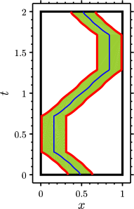
Refer to caption Refer to caption Refer to caption Refer to caption
Figure 8: (EX2) - From left to right, optimal control domain, isovalues of the corresponding adjoint state φ𝜑\varphi, isovalues of the uncontrolled and controlled wave over the optimal domain, for the initial curve γ01/2subscript𝛾012\gamma_{0}\equiv 1/2.

The evolution of the cost Jϵnsuperscriptsubscript𝐽italic-ϵ𝑛J_{\epsilon}^{n} and the derivative dJϵn𝑑superscriptsubscript𝐽italic-ϵ𝑛dJ_{\epsilon}^{n} with respect to n𝑛n are displayed in Figure 9. Figure 6-Right depicts the values of the functional Jϵsubscript𝐽italic-ϵJ_{\epsilon} for the constant curves γx0𝛾subscript𝑥0\gamma\equiv x_{0} used to determine the best cylindrical domain and highlights the low variation of the cost with respect to the position of such domains.
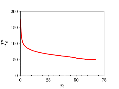
Refer to caption Refer to caption
Figure 9: (EX2) - Evolution of the cost Jϵnsuperscriptsubscript𝐽italic-ϵ𝑛J_{\epsilon}^{n} (left) and the derivative dJϵn𝑑superscriptsubscript𝐽italic-ϵ𝑛dJ_{\epsilon}^{n} (right) for the initial curve γ01/2subscript𝛾012\gamma_{0}\equiv 1/2.

\bullet We now consider the initial datum (y0,y1)subscript𝑦0subscript𝑦1(y_{0},y_{1}) given by

y0(x)=(10x4)2(10x6)2𝟙[0.4,0.6](x),y1(x)=0,for x(0,1).formulae-sequencesubscript𝑦0𝑥superscript10𝑥42superscript10𝑥62subscript10.40.6𝑥formulae-sequencesubscript𝑦1𝑥0for 𝑥01y_{0}(x)=(10x-4)^{2}(10x-6)^{2}\mathbbm{1}_{[0.4,0.6]}(x),\quad y_{1}(x)=0,\qquad\text{for }x\in(0,1). (EX3)

This initial condition generates two travelling waves going in opposite directions, as can be seen in Figure 10.3. For T=2𝑇2T=2, ϵ=102italic-ϵsuperscript102\epsilon=10^{-2} and ρ=104𝜌superscript104\rho=10^{-4}, we initialize the algorithm with the initial curve γ01/2subscript𝛾012\gamma_{0}\equiv 1/2. The convergence is observed after 111111111 iterations leading to Jϵ(γopt)41.02subscript𝐽italic-ϵsubscript𝛾opt41.02J_{\epsilon}(\gamma_{\text{opt}})\approx 41.02. Moreover, the minimal cost for cylindrical domains is minx0Jϵ(x0)85.08subscriptsubscript𝑥0subscript𝐽italic-ϵsubscript𝑥085.08\min_{x_{0}}J_{\epsilon}(x_{0})\approx 85.08, so that the performance index is Π(γopt)51.79Πsubscript𝛾opt51.79\Pi(\gamma_{\text{opt}})\approx 51.79%. Once again, our non-cylindrical setup is much more efficient than the cylindrical one. It is still due to the fact that the domains we consider can follow the propagation of the travelling waves, one after the other. This can be noticed in Figure 10, where we display the optimal control domain, the corresponding adjoint state φ𝜑\varphi, the uncontrolled and the controlled wave over the optimal domain.
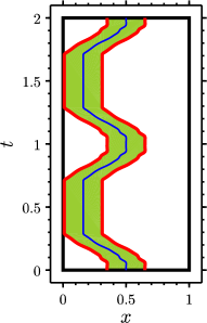
Refer to caption Refer to caption Refer to caption Refer to caption
Figure 10: (EX3) - From left to right, optimal control domain, isovalues of the corresponding adjoint state φ𝜑\varphi, isovalues of the uncontrolled and controlled wave over the optimal domain, for T=2𝑇2T=2, for the initial curve γ01/2subscript𝛾012\gamma_{0}\equiv 1/2.

In order to show the influence of the controllability time on the optimal domain, for ϵ=102italic-ϵsuperscript102\epsilon=10^{-2} and γ01/2subscript𝛾012\gamma_{0}\equiv 1/2, we use the descent algorithm with T=1𝑇1T=1 and ρ=2.5×10⁵𝜌2.5superscript105\rho=2.5\times 10^{-5}, initialized with the curve γ0=1/2subscript𝛾012\gamma_{0}=1/2. Remark that the corresponding domain do satisfies the geometric optic condition. The convergence is observed after 213213213 iterations and the optimal cost is Jϵ(γopt)94.78subscript𝐽italic-ϵsubscript𝛾opt94.78J_{\epsilon}(\gamma_{\text{opt}})\approx 94.78. Moreover, the minimal cost for cylindrical domains is minx0Jϵ(x0)183.98subscriptsubscript𝑥0subscript𝐽italic-ϵsubscript𝑥0183.98\min_{x_{0}}J_{\epsilon}(x_{0})\approx 183.98, so that the performance index is Π(γopt)48.48Πsubscript𝛾opt48.48\Pi(\gamma_{\text{opt}})\approx 48.48%. Observe that the cylindrical domains associated with x0(0.25,0.75)subscript𝑥00.250.75x_{0}\notin(0.25,0.75) do not verify the geometric optics condition. This highlights the necessity to use non-cylindrical domains. Compared to the simulation for T=2𝑇2T=2, the optimal cost increases by a factor around 2.32.32.3. Figure 11 displays the optimal control domain, the corresponding adjoint state φ𝜑\varphi, the uncontrolled and controlled wave over the optimal domain. We remark that the projection of the optimal domain on the x𝑥x-axis covers the whole domain ΩΩ\Omega, in contrast with the domain associated with T=2𝑇2T=2.

Refer to caption Refer to caption Refer to caption Refer to caption
Figure 11: (EX3) - From left to right, optimal control domain, isovalues of the corresponding adjoint state φ𝜑\varphi, isovalues of the uncontrolled and controlled wave over the optimal domain, for T=1𝑇1T=1, for the initial curve γ01/2subscript𝛾012\gamma_{0}\equiv 1/2.

\bullet Eventually, in order to highlight the influence of the regularization parameter ϵitalic-ϵ\epsilon on the optimal domain, we now consider the initial datum (y0,y1)subscript𝑦0subscript𝑦1(y_{0},y_{1}) given by

y0(x)={3xif 0x1/3,3(12x)if 1/3x2/3,3(1x)if 2/3x1,y1(x)=0,for x(0,1).formulae-sequencesubscript𝑦0𝑥cases3𝑥if 0𝑥13312𝑥if 13𝑥2331𝑥if 23𝑥1formulae-sequencesubscript𝑦1𝑥0for 𝑥01y_{0}(x)=\left\{\begin{array}[]{cl}3x&\text{if }0\leq x\leq 1/3,\\ 3(1-2x)&\text{if }1/3\leq x\leq 2/3,\\ -3(1-x)&\text{if }2/3\leq x\leq 1,\end{array}\right.\quad y_{1}(x)=0,\qquad\text{for }x\in(0,1). (EX4)

For T=2𝑇2T=2 and ρ=105𝜌superscript105\rho=10^{-5}, we initialize the descent algorithm with the curve γ1/2𝛾12\gamma\equiv 1/2 and consider ϵ=102italic-ϵsuperscript102\epsilon=10^{-2} and ϵ=0italic-ϵ0\epsilon=0. The numbers of iterations until convergence, the values of the functional Jϵsubscript𝐽italic-ϵJ_{\epsilon} evaluated at the optimal curve γoptsubscript𝛾opt\gamma_{\text{opt}} and the performance indices of γoptsubscript𝛾opt\gamma_{\text{opt}} are listed in Table 3. For the initial datum (EX4), the minimal cost for cylindrical domains is minx0Jϵ(x0)47.71subscriptsubscript𝑥0subscript𝐽italic-ϵsubscript𝑥047.71\min_{x_{0}}J_{\epsilon}(x_{0})\approx 47.71.

ϵitalic-ϵ\epsilon 00 102superscript10210^{-2}
Number of iterations 247247247 389389389
Jϵ(γopt)subscript𝐽italic-ϵsubscript𝛾optJ_{\epsilon}(\gamma_{\text{opt}}) 60.3560.3560.35 43.2343.2343.23
Π(γopt)Πsubscript𝛾opt\Pi(\gamma_{\text{opt}}) 26.5126.51-26.51% 9.389.389.38%
Table 3: (EX4) - Number of iterations, optimal value of the functional Jϵsubscript𝐽italic-ϵJ_{\epsilon} and performance index, for ϵ{0,102}italic-ϵ0superscript102\epsilon\in\{0,10^{-2}\}, for the initial curve γ01/2subscript𝛾012\gamma_{0}\equiv 1/2.

In Figure 12, we clearly see the regularizing effect of ϵitalic-ϵ\epsilon and the need of regularization in this case, as the optimal domain obtained when ε=0𝜀0\varepsilon=0 is very oscillating.

Refer to caption Refer to caption Refer to caption Refer to caption
Figure 12: (EX4) - Optimal control domain and isovalues of the adjoint state for ϵ=102italic-ϵsuperscript102\epsilon=10^{-2} (left), ϵ=0italic-ϵ0\epsilon=0 (right), for the initial curve γ01/2subscript𝛾012\gamma_{0}\equiv 1/2.

4.2 Iterative approximation of the observability constant

In this last part, we formally describe and use an algorithm allowing to approximate the observability constant appearing in (3), associated to any domain qQT𝑞subscript𝑄𝑇q\subset Q_{T}. The algorithm is based on the following characterization:

Cobs(q)=sup𝐲0𝐕RΛq𝐲0,𝐲0𝐕𝐲0𝐕2.subscript𝐶obs𝑞subscriptsupremumsubscript𝐲0𝐕subscript𝑅subscriptΛ𝑞subscript𝐲0subscript𝐲0𝐕superscriptsubscriptnormsubscript𝐲0𝐕2C_{\text{obs}}(q)=\sup_{\mathbf{y}_{0}\in\mathbf{V}}\frac{\langle R\Lambda_{q}\mathbf{y}_{0},\mathbf{y}_{0}\rangle_{\mathbf{V}}}{\|\mathbf{y}_{0}\|_{\mathbf{V}}^{2}}. (58)

where ΛqsubscriptΛ𝑞\Lambda_{q} and R𝑅R are respectively the control operator associated to the domain q𝑞q and the duality operator between the space 𝐖𝐖\mathbf{W} and 𝐕𝐕\mathbf{V}:

Λq:{𝐕𝐖𝐲0𝝋^0,R:{𝐖𝐕(φ0,φ1)((x2)1φ1,φ0).:subscriptΛ𝑞cases𝐕𝐖subscript𝐲0maps-tosubscript^𝝋0𝑅:cases𝐖𝐕subscript𝜑0subscript𝜑1maps-tosuperscriptsubscriptsuperscript2𝑥1subscript𝜑1subscript𝜑0\Lambda_{q}:\left\{\begin{array}[]{ccc}\mathbf{V}&\to&\mathbf{W}\\ \mathbf{y}_{0}&\mapsto&\widehat{\boldsymbol{\varphi}}_{0}\end{array}\right.,\qquad R:\left\{\begin{array}[]{ccc}\mathbf{W}&\to&\mathbf{V}\\ (\varphi_{0},\varphi_{1})&\mapsto&((-\partial^{2}_{x})^{-1}\varphi_{1},-\varphi_{0})\end{array}\right.. (59)

In the definition of ΛqsubscriptΛ𝑞\Lambda_{q}, 𝝋^0𝐖subscript^𝝋0𝐖\widehat{\boldsymbol{\varphi}}_{0}\in\mathbf{W} is the minimum of the functional 𝒥superscript𝒥\mathcal{J}^{\star} (cf. (5)) associated to 𝐲0𝐕subscript𝐲0𝐕\mathbf{y}_{0}\in\mathbf{V}. The characterization (58) can be obtained by following the steps of [20, Section 2] and [6, Remark 2.98]. The main consequence of this characterization is that Cobs(q)subscript𝐶obs𝑞C_{\text{obs}}(q) can be viewed as the largest eigenvalue of the operator RΛq𝑅subscriptΛ𝑞R\Lambda_{q} in 𝐕𝐕\mathbf{V}. Consequently, we can formally adapt the power iteration method to our infinite-dimensional setting. The algorithm reads as follows. Let 𝐲00𝐕superscriptsubscript𝐲00𝐕\mathbf{y}_{0}^{0}\in\mathbf{V} be given such that 𝐲00𝐕=1subscriptnormsuperscriptsubscript𝐲00𝐕1\|\mathbf{y}_{0}^{0}\|_{\mathbf{V}}=1. For n0𝑛0n\geq 0, using the space-time finite element method described in [3, Section 3-4], we compute 𝝋^0n=Λq𝐲0nsuperscriptsubscript^𝝋0𝑛subscriptΛ𝑞superscriptsubscript𝐲0𝑛\widehat{\boldsymbol{\varphi}}_{0}^{n}=\Lambda_{q}\mathbf{y}_{0}^{n} then set 𝐳0n=R𝝋^0nsuperscriptsubscript𝐳0𝑛𝑅superscriptsubscript^𝝋0𝑛\mathbf{z}_{0}^{n}=R\widehat{\boldsymbol{\varphi}}_{0}^{n} and 𝐲0n+1=𝐳0n/𝐳0n𝐕superscriptsubscript𝐲0𝑛1superscriptsubscript𝐳0𝑛subscriptnormsuperscriptsubscript𝐳0𝑛𝐕\mathbf{y}_{0}^{n+1}=\mathbf{z}_{0}^{n}/\|\mathbf{z}_{0}^{n}\|_{\mathbf{V}}. We finally have Cobs(q)=limn𝐳0n𝐕subscript𝐶obs𝑞subscript𝑛subscriptnormsuperscriptsubscript𝐳0𝑛𝐕C_{\text{obs}}(q)=\lim_{n\to\infty}\|\mathbf{z}_{0}^{n}\|_{\mathbf{V}} while 𝐲0nsuperscriptsubscript𝐲0𝑛\mathbf{y}_{0}^{n} converges in 𝐕𝐕\mathbf{V} to the most expensive initial datum to control. For the control domain of Figure 3, this algorithm (after an appropriate space-time), initialized with 𝐲00=K(x(1x),0)superscriptsubscript𝐲00𝐾𝑥1𝑥0\mathbf{y}_{0}^{0}=K(x(1-x),0) - K𝐾K such that 𝐲00𝐕=1subscriptnormsuperscriptsubscript𝐲00𝐕1\|\mathbf{y}_{0}^{0}\|_{\mathbf{V}}=1-, produces the following sequence {𝐳0n𝐕}n0={2.6895,3.829,3.981,3.994,3.997,}subscriptsubscriptnormsuperscriptsubscript𝐳0𝑛𝐕𝑛02.68953.8293.9813.9943.997\{\|\mathbf{z}_{0}^{n}\|_{\mathbf{V}}\}_{n\geq 0}=\{2.6895,3.829,3.981,3.994,3.997,\cdots\} converging toward the value 444, in agreement with the result of Section 2.3 based on a graph argument. The most expensive initial datum to control is displayed in Figure 13. Remark that the initial datum solution of (58) is not unique.
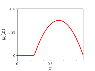
Refer to caption Refer to caption
Figure 13: Most expensive initial data y0subscript𝑦0y_{0} (left) and y1subscript𝑦1y_{1} (right) to be controlled.

5 Conclusion and perspectives

Making use of the d’Alembert formulae for the solutions of the one dimensional wave equation, we have shown a uniform observability inequality with respect to the class of non cylindrical domains satisfying the geometric optics condition. The proof based on arguments from graph theory allows notably to relate the value of the observability constant to the spectrum of the Laplacian matrix, defined in term of the graph of any domain qQT𝑞subscript𝑄𝑇q\subset Q_{T}. The uniform observability property then allows to consider and analyze the problem of the control’s optimal support associated to fixed initial conditions. For simplicity, the optimization is made over connected domains defined by regular curves. As expected, the optimal domains (approximated within a space-time finite element method) are closely related to the travelling waves generated by the initial conditions.

This work may be extended in several directions. First, the characterization of the observability constant in term of a computable eigenvalue problem in Section 4.2 may allow to consider the optimization of such constant with respect to the domain of observation, i.e. infq𝒬adεCobs(q)subscriptinfimum𝑞superscriptsubscript𝒬ad𝜀subscript𝐶obs𝑞\inf_{q\in\mathcal{Q}_{\text{ad}}^{\varepsilon}}C_{\text{obs}}(q). Moreover, from an approximation point of view, we may also consider more general domains (than connected ones) and use, for instance, a level set method to describe the geometry (as done in [18]). Eventually, this work may be adapted to the case of controls supported on single curves of QTsubscript𝑄𝑇Q_{T}, using the uniform observability property given in [2].

The extension of this work to the N𝑁N-dimensional case studied in [13, 22] is also a challenge.

References

  • [1] A. E. Brouwer and W. H. Haemers, Spectra of graphs, Universitext, Springer, New York, 2012.
  • [2] C. Castro, Exact controllability of the 1-D wave equation from a moving interior point, ESAIM Control Optim. Calc. Var., 19 (2013), pp. 301–316.
  • [3] C. Castro, N. Cîndea, and A. Münch, Controllability of the linear one-dimensional wave equation with inner moving forces, SIAM J. Control Optim., 52 (2014), pp. 4027–4056.
  • [4] F. R. K. Chung, Spectral graph theory, vol. 92 of CBMS Regional Conference Series in Mathematics, Published for the Conference Board of the Mathematical Sciences, Washington, DC; by the American Mathematical Society, Providence, RI, 1997.
  • [5] N. Cîndea and A. Münch, A mixed formulation for the direct approximation of the control of minimal L2superscript𝐿2L^{2}-norm for linear type wave equations, Calcolo, 52 (2015), pp. 245–288.
  • [6] J.-M. Coron, Control and nonlinearity, vol. 136 of Mathematical Surveys and Monographs, American Mathematical Society, Providence, RI, 2007.
  • [7] L. Cui, X. Liu, and H. Gao, Exact controllability for a one-dimensional wave equation in non-cylindrical domains, J. Math. Anal. Appl., 402 (2013), pp. 612–625.
  • [8] B. H. Haak and D.-T. Hoang, Exact observability of a 1-dimensional wave equation on a noncylindrical domain, SIAM J. Control Optim., 57 (2019), pp. 570–589.
  • [9] F. Hecht, New development in Freefem++, J. Numer. Math., 20 (2012), pp. 251–265.
  • [10] A. Henrot and M. Pierre, Variation et optimisation de formes, vol. 48 of Mathématiques & Applications (Berlin) [Mathematics & Applications], Springer, Berlin, 2005. Une analyse géométrique. [A geometric analysis].
  • [11] E. Humbert, Y. Privat, and E. Trélat, Observability properties of the homogeneous wave equation on a closed manifold, Comm. Partial Differential Equations, 44 (2019), pp. 749–772.
  • [12] A. Y. Khapalov, Controllability of the wave equation with moving point control, Appl. Math. Optim., 31 (1995), pp. 155–175.
  • [13] J. Le Rousseau, G. Lebeau, P. Terpolilli, and E. Trélat, Geometric control condition for the wave equation with a time-dependent observation domain, Anal. PDE, 10 (2017), pp. 983–1015.
  • [14] J.-L. Lions, Contrôlabilité exacte, perturbations et stabilisation de systèmes distribués. Tome 1, vol. 8 of Recherches en Mathématiques Appliquées [Research in Applied Mathematics], Masson, Paris, 1988. Contrôlabilité exacte. [Exact controllability], With appendices by E. Zuazua, C. Bardos, G. Lebeau and J. Rauch.
  • [15] K. Liu and J. Yong, Rapid exact controllability of the wave equation by controls distributed on a time-variant subdomain, Chinese Ann. Math. Ser. B, 20 (1999), pp. 65–76. A Chinese summary appears in Chinese Ann. Math. Ser. A 20 (1999), no. 1, 142.
  • [16] P. Martin, L. Rosier, and P. Rouchon, Null controllability of the structurally damped wave equation with moving control, SIAM J. Control Optim., 51 (2013), pp. 660–684.
  • [17] B. Mohar, The Laplacian spectrum of graphs, in Graph theory, combinatorics, and applications. Vol. 2 (Kalamazoo, MI, 1988), Wiley-Intersci. Publ., Wiley, New York, 1991, pp. 871–898.
  • [18] A. Münch, Optimal design of the support of the control for the 2-D wave equation: a numerical method, Int. J. Numer. Anal. Model., 5 (2008), pp. 331–351.
  • [19]  , Optimal location of the support of the control for the 1-D wave equation: numerical investigations, Comput. Optim. Appl., 42 (2009), pp. 443–470.
  • [20]  , Numerical estimations of the cost of boundary controls for the equation ytεyxx+Myx=0subscript𝑦𝑡𝜀subscript𝑦𝑥𝑥𝑀subscript𝑦𝑥0y_{t}-\varepsilon y_{xx}+My_{x}=0 with respect to ε𝜀\varepsilon, in Recent advances in PDEs: analysis, numerics and control, vol. 17 of SEMA SIMAI Springer Ser., Springer, Cham, 2018, pp. 159–191.
  • [21] F. Periago, Optimal shape and position of the support for the internal exact control of a string, Systems Control Lett., 58 (2009), pp. 136–140.
  • [22] A. Shao, On Carleman and observability estimates for wave equations on time-dependent domains, Proc. Lond. Math. Soc. (3), 119 (2019), pp. 998–1064.