BIMC: The Bayesian Inverse Monte Carlo method for goal-oriented uncertainty quantification. Part II.

Abstract

In Part I of this article, we proposed an importance sampling algorithm to compute rare-event probabilities in forward uncertainty quantification problems. The algorithm, which we termed the “Bayesian Inverse Monte Carlo (BIMC) method”, was shown to be optimal for problems in which the input-output operator is nearly linear. But applying the original BIMC to highly nonlinear systems can lead to several different failure modes. In this paper, we modify the BIMC method to extend its applicability to a wider class of systems. The modified algorithm, which we call “Adaptive-BIMC (A-BIMC)”, has two stages. In the first stage, we solve a sequence of optimization problems to roughly identify those regions of parameter space which trigger the rare-event. In the second stage, we use the stage one results to construct a mixture of Gaussians that can be then used in an importance sampling algorithm to estimate rare event probability. We propose using a local surrogate that minimizes costly forward solves. The effectiveness of A-BIMC is demonstrated via several synthetic examples. Yet again, the modified algorithm is prone to failure. We systematically identify conditions under which it fails to lead to an effective importance sampling distribution.

65C05, 62P30

1 Introduction

Part I of this paper presented an importance sampling algorithm to address the following goal-oriented uncertainty quantification (UQ) question. Given

• a smooth nonlinear function $f(\bm{x}):\mathbb{R}^{m}\rightarrow\mathbb{R}$,

• a probability distribution for its inputs $p(\bm{x})$, and,

• a target interval $\mathbb{Y}\subset\mathbb{R}$,

what is the probability of the event $f(\bm{x})\in\mathbb{Y}$? Our interest was in computing this probability efficiently, i.e., with as few evaluations of $f$ as possible, especially when the event $f(\bm{x})\in\mathbb{Y}$ is rare.

The algorithm presented in Part I, called the Bayesian Inverse Monte Carlo (BIMC) method, employed a fictitious Bayesian inverse problem to identify regions of parameter space that evaluate inside $\mathbb{Y}$. BIMC was proven to lead to an optimal IS density for affine $f$ and Gaussian $p$. As such, when applied to maps $f$ that appear nearly affine at the scale of the covariance of $p$, BIMC outperformed a simple Monte Carlo method by several orders of magnitude.

We also showed that when this is not the case, that is, when $f$ is significantly nonlinear, BIMC leads to a poor-quality IS distribution. This in turn can lead to inaccurate estimates of the rare-event probability. In Part II of this two-part article, we propose modifications to BIMC in order to address this major limitation.

Summary of the methodology

The modifications result in a two-stage algorithm, which we christen Adaptive-BIMC (A-BIMC). Stage-1 of A-BIMC solves a sequence of optimization problems in order to adaptively explore the input parameter space where $f(\bm{x})\in\mathbb{Y}$ (more precisely, this region is the pre-image of $\mathbb{Y}$, defined as the set $\{\bm{x}\in\mathbb{R}^{m}:f(\bm{x})\in\mathbb{Y}\}$ and denoted $f^{-1}(\mathbb{Y})$). While BIMC also relies on the solution of an auxiliary, “fictitious”, inverse problem, the formulation and interpretation of the optimization problems in Stage-1 of A-BIMC is quite different.

BIMC solves a single optimization problem to arrive at a pseudo-MAP point and then samples around this point to explore the pre-image $f^{-1}(\mathbb{Y})$. By sampling around a single point, BIMC only achieves local exploration of $f^{-1}(\mathbb{Y})$. While this may work for nearly affine maps, such limited exploration is insufficient for more nonlinear problems.

On the other hand, Stage-1 of A-BIMC solves optimization problems in an iterative fashion; the optimization problem in some iteration, aided by specially designed algorithmic components, explores the pre-image $f^{-1}(\mathbb{Y})$ away from regions explored in the preceding iterations. This allows global exploration of $f^{-1}(\mathbb{Y})$. Stage-1 keeps iterating till a termination condition based on user-specified tolerances is met. Then, the local minima so obtained are collected into a Gaussian mixture that roughly approximates the theoretically ideal (zero-error) importance sampling density $q^{*}\propto\bm{\mathrm{1}}_{\mathbb{Y}}(f(\bm{x}))p(\bm{x})$.

The Gaussian mixture which crudely approximates $q^{*}$ is refined using the Mixture Population Monte Carlo Algorithm [2]. The MPMC algorithm modifies the mixture weights, means, and covariances of this Gaussian mixture so that it closely approximates the ideal IS density $q^{*}$. This, however, requires further evaluations of $f$, raising the computational cost of the algorithm. In order to circumvent this problem, we replace evaluations of $f$ in $q^{*}$ with that of a heuristically constructed surrogate of $f$. Next, we list the contributions and limitations of our approach.

Contributions

• We extend our work in Part I and propose a novel scheme which adaptively explores the pre-image $f^{-1}(\mathbb{Y})$ on a global scale. In particular, we describe algorithmic strategies, such as parameter continuation, and a modified penalty algorithm required to achieve this exploration.

• Our scheme employs the derivatives of $f$ to accelerate exploration of the pre-image $f^{-1}(\mathbb{Y})$, as opposed to only pointwise evaluations of $f$.

• We have attempted to keep tunable algorithmic parameters to a minimum, and as a result, A-BIMC possesses just one user-defined parameter.

• A-BIMC’s performance is studied on synthetic problems. Experiments demonstrate that the performance of our method doesn’t depend significantly on how small the target probability is. Rather it depends on the nonlinearity of the input-output map.

Limitations

• A-BIMC is a purely heuristic algorithm. In particular, the algorithmic components chosen preclude its theoretical analysis. Hence, unlike BIMC, it is difficult to a-prior predict its performance.

• A-BIMC is not without its own failure mechanisms. These are described in Section 5, along with strategies for diagnosing and mitigating them.

• While our algorithm possesses only one tunable parameter, we don’t have an a priori prescription for choosing it. We recommend a default value in Section 4 but cannot provide guarantees on whether this value will work or not.

• A-BIMC relies crucially on the MPMC method, which doesn’t scale to high-dimensional problems (say, for instance, greater than 64). As a result, A-BIMC is not suitable for problems with high intrinsic dimension.

Notation

Key notation used in this paper is summarized in Table 1.

Symbols/Acronyms	Meaning
MC	Monte Carlo
IS	Importance Sampling
BIMC	Bayesian Inverse Monte Carlo
A-BIMC	Adaptive Bayesian Inverse Monte Carlo
ESS	Effective Sample Size
MPMC	Mixture Population Monte Carlo
RMS	Root Mean Square
MAP	Maximum A Posteriori
$f$	input-output, or the forward, map
$\bm{x}$	vector of input parameters to $f$
$p(\bm{x})$	input or nominal probability density for $\bm{x}$
$\mathbb{Y}$	target interval for $f(\bm{x})$
$\bm{\mathrm{1}}_{\mathbb{Y}}$	indicator function, $\bm{\mathrm{1}}_{\mathbb{Y}}(z)$ is 1 if $z\in\mathbb{Y}$, 0 otherwise
$f^{-1}(\mathbb{Y})$	pre-image of the interval $\mathbb{Y}$, $\{\bm{x}\in\mathbb{R}^{m}:f(\bm{x})\in\mathbb{Y}\}$
$m$	dimension of $\bm{x}$
$\mathcal{N}\left(\bm{x}_{0},\bm{\Sigma}_{0}\right)$	normal distribution with mean $\bm{x}_{0}$ and covariance $\bm{\Sigma}_{0}$
$\mathbb{P}$	probability of an event
$\mathbb{E}_{p}$	expectation of a random variable with respect to some density $p$
$\mathbb{V}_{p}$	variance of a random variable with respect to some density $p$
$\mu$	$\mathbb{P}\left(f(\bm{x})\in\mathbb{Y}\right)$, equivalently, $\mathbb{E}_{p}\left(\bm{\mathrm{1}}_{\mathbb{Y}}\left(f(\bm{x})\right)\right)$.
$q^{*}$	ideal importance sampling density
$Q_{k}$	importance sampling mixture density at the $k$-th iteration of Stage-1
$Q$	final importance sampling mixture density
$N$	number of samples
$\hat{\mu}^{N}$	MC estimate for $\mu$ computed using $N$ samples
$\tilde{\mu}^{N}$	IS estimate for $\mu$ computed using $N$ samples
$\hat{e}_{\mathrm{RMS}}^{N}$	RMS error in $\hat{\mu}^{N}$
$\tilde{e}_{\mathrm{RMS}}^{N}$	RMS error in $\tilde{\mu}^{N}$
$y$	pseudo-data
$p(y|\bm{x})$	pseudo-likelihood density
$p(\bm{x}|y)$	pseudo-posterior density
$\bm{x}_{\mathrm{MAP}}$	MAP point of $p(\bm{x}|y)$
$\mathbf{H}_{\mathrm{MAP}}$	Hessian of $-\log p(\bm{x}|y)$ at $\bm{x}_{\mathrm{MAP}}$
$\mathbf{H}_{\mathrm{GN}}$	Gauss-Newton Hessian of $-\log p(\bm{x}|y)$ at some $\bm{x}$
$\epsilon_{\mathrm{rel}}$	relative tolerance for perplexity change across A-BIMC iterations
$\epsilon_{\mathrm{abs}}$	absolute tolerance for perplexity change across A-BIMC iterations
$f_{\mathrm{surrogate}}$	cheap-to-evaluate surrogate for $f$
$N_{\mathrm{MPMC}}$	number of samples used by MPMC
$m_{\mathrm{int}}$	intrinsic dimension of the rare-event problem
$D_{\mathrm{KL}}(p||q)$	Kullback-Leibler (KL) divergence between densities $p$ and $q$

Table 1: Summary of key notation used in this paper.

Outline of the paper

In Section 2, we briefly review the BIMC method, drawing attention to the core theoretical ideas behind it, as well as its failure mechanisms. We describe A-BIMC in detail in Section 3. A-BIMC’s performance is studied via several numerical experiments in Section 4. In Section 5, we discuss how A-BIMC can fail, and provide strategies for diagnosing and mitigating failure. We conclude in Section 6 and discuss several avenues for future research. Supporting theory and additional results accompanying our computational experiments are provided in the supplement [14].

2 BIMC

To provide context and motivation for developing A-BIMC, this section provides a brief review of the BIMC algorithm. BIMC identifies regions of parameter space that evaluate inside $\mathbb{Y}$ by setting up a fictitious inverse problem. This fictitious inverse problem is defined by re-interpreting the ingredients of the posed rare-event probability estimation problem (namely, $f(\bm{x})$, $p(\bm{x})$, and $\mathbb{Y}$) in the following manner:

1. some $y\in\mathbb{Y}$ is selected to represent the observations,

2. $p(\bm{x})$ is interpreted as the prior, and,

3. a likelihood model, assuming additive Gaussian error of some magnitude $\sigma$ is constructed.

These ingredients lead to a fictitious posterior distribution, $p(\bm{x}|y)\propto p(y|\bm{x})p(\bm{x})$. BIMC obtains an IS density $q(\bm{x})$ by approximating the fictitious posterior $p(\bm{x}|y)$ with a Gaussian distribution. The Gaussian approximation invokes Laplace’s method [7, 15]. to yield $q(\bm{x})=\mathcal{N}\left(\bm{x}_{\mathrm{MAP}},\mathbf{H}_{\mathrm{MAP}}^{-1}\right)$, where $\bm{x}_{\mathrm{MAP}}$ is the maximum a posteriori point of $p(\bm{x}|y)$, and $\mathbf{H}_{\mathrm{MAP}}$ is the Hessian matrix of $-\log p(\bm{x}|y)$ at $\bm{x}_{\mathrm{MAP}}$. In this procedure, the inference problem is termed fictitious because both the observation $y$ and the likelihood variance $\sigma^{2}$ are auxiliary variables that are selected by the algorithm. This inverse problem is solved for the sole purpose of constructing an effective importance sampling density.

Being contrived quantities, appropriate values for the pseudo-data $y$ and pseudo-likelihood variance $\sigma^{2}$ are not known a priori. However, they can have a profound impact on the performance of the importance sampling distribution and must be tuned with care. The tuning procedure that BIMC adopts is reproduced in the next subsection.

2.1 Tuning parameters

In BIMC, the strategy for tuning $\sigma^{2}$ and $y$ is based on theoretical analysis of the case when $f(\bm{x})$ when affine and $p(\bm{x})$ is Gaussian. Suppose that this is indeed so, that is, $f(\bm{x})=\bm{v}^{T}\bm{x}+\beta$, $p(\bm{x})=\mathcal{N}(\bm{x}_{0},\mathbf{\Sigma}_{0})$ for some $\bm{v}$, $\bm{x}_{0}\in\mathbb{R}^{m}$, $\beta\in\mathbb{R}$ and $\mathbf{\Sigma}_{0}\in\mathbb{R}^{m\times m}$. Then, for some pseudo-data $y\in\mathbb{R}$ and pseudo-likelihood variance $\sigma^{2}\in\mathbb{R}^{+}$, the expression for the IS density is: $q(\bm{x})=\mathcal{N}(\bm{x}_{\mathrm{MAP}},\mathbf{H}_{\mathrm{MAP}}^{-1})$, where,

(1) $$\bm{x}_{\mathrm{MAP}}=\bm{x}_{0}+\frac{y-f(\bm{x}_{0})}{\sigma^{2}+\bm{v}^{T}\mathbf{\Sigma}_{0}\bm{v}}\mathbf{\Sigma}_{0}\bm{v},\quad\mathbf{H}_{\mathrm{MAP}}^{-1}=\mathbf{\Sigma}_{0}-\frac{1}{\sigma^{2}+\bm{v}^{T}\mathbf{\Sigma}_{0}\bm{v}}\big{(}\mathbf{\Sigma}_{0}\bm{v}\big{)}{\big{(}\mathbf{\Sigma}_{0}\bm{v}\big{)}}^{T}.$$

Recall that an efficient IS density is one that is similar to $q^{*}$. Hence, it follows that suitable values for $\sigma^{2}$ and $y$ are those that make $q(\bm{x})$, as parameterized by $\sigma^{2}$ and $y$, resemble $q^{*}$ the most. These optimal values for $\sigma^{2}$ and $y$ can be found by minimizing the Kullback-Leibler (KL) divergence between $q^{*}$ and $q$:

(2) $$\begin{pmatrix}\sigma^{*}\\ y^{*}\end{pmatrix} =\operatorname*{arg\,min}_{\sigma,y}D_{\mathrm{KL}}(q^{*}||q;\sigma,y)$$

In the affine-Gaussian case, $D_{\mathrm{KL}}(q^{*}||q)$, $\sigma^{*}$, and $y^{*}$ have analytical expressions. Part 1 of this paper derived these expressions and proved that in the affine-Gaussian case, $q(\bm{x};\sigma^{*},y^{*})$ is the Gaussian distribution closest in KL divergence to $q^{*}$. For situations where the input-output map is not affine, closed form expressions for $q(\bm{x};\sigma,y)$ and $D_{\mathrm{KL}}(q^{*}||q;\sigma,y)$ can rarely be written down. BIMC tunes the parameters $\sigma^{2}$ and $y$ in such cases by first linearizing $f(\bm{x})$ around a suitable point. Linearization yields an affine approximation of $f$ which is plugged into the procedure described above. Although this yields parameters that are optimal for the affine approximation and not for the full nonlinear problem, it precludes additional calls to $f(\bm{x})$, thus keeping computational costs low.

This methodology to devise an efficient IS density can fail in several cases. These failure cases are detailed next.

Figure 1: A single Gaussian distribution fails to cover curved and/or disjoint $f^{-1}(\mathbb{Y})$ when $f(\bm{x})=\sin(x_{1})\cos(x_{2})$. Shown are 5000 samples from $q^{*}$ and 500 MC and BIMC samples.

2.2 Failure modes of BIMC

The failure modes of BIMC can be categorized broadly into four cases:

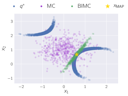
• Curvature of $f^{-1}(\mathbb{Y})$: Since BIMC results in an optimal approximation of $q^{*}(\bm{x})$ in the affine-Gaussian case, it is expected to perform well for input-output maps that are nearly affine. Using BIMC when this is not the case is susceptible to failure, an unsurprising fact; using a single Gaussian distribution, with convex, elliptical contours may prove to be insufficient to cover arbitrary $f^{-1}(\mathbb{Y})$. This phenomenon is captured in Figure 1 where $f:\mathbb{R}^{2}\rightarrow\mathbb{R}$ is defined as $f(\bm{x})=\sin(x_{1})\cos(x_{2})$ and the pre-image $f^{-1}(\mathbb{Y})$ is a circular region in space. In conclusion, this mode of failure occurs when $f(\bm{x})$ is strongly nonlinear at the scale of the covariance of $p(\bm{x})$.

• Multiply-connected $f^{-1}(\mathbb{Y})$: BIMC can also fail if $f^{-1}(\mathbb{Y})$ is the union of disjoint regions in space, which is also evident in Figure 1. In this case, $q^{*}$ has multiple modes whereas a single Gaussian can only capture one. Because the mean of $q(\bm{x})$ is found using numerical optimization, which mode is found depends on the initial guess provided to the numerical optimization routine.

• Poor selection of tunable parameters: Yet another failure mode occurs when the optimal tunable parameters that result from linearizing $f$ aren’t appropriate for the full nonlinear problem. As Equation 1 reveals, the covariance of $q(\bm{x})$ is a rank-1 non-positive definite update of the covariance of $p(\bm{x})$. The degree of this update is inversely proportional to $\sigma^{2}$. If the optimal likelihood variance, $\sigma^{2}$, for the linearized problem is much smaller than the optimal likelihood variance for the full nonlinear problem, the covariance update will be needlessly large, and consequently, $q(\bm{x})$ will not have enough support to cover $f^{-1}(\mathbb{Y})$. This can cause large IS ratios, and at small to moderate sample sizes, biased estimates for the rare event probability.

• Intractable inverse problem: It may be the case that the optimization problem formulated to compute $\bm{x}_{\mathrm{MAP}}$ is highly ill-conditioned and non-convex, making $\bm{x}_{\mathrm{MAP}}$ inaccessible via standard numerical optimization routines. Since the BIMC methodology is crucially dependent on successfully computing $\bm{x}_{\mathrm{MAP}}$, we declare failure if the numerical optimization routine employed fails at its task.

This concludes our recap of the BIMC method and its limitations. The next section develops the Adaptive-BIMC (A-BIMC) methodology in detail.

3 Methodology

A-BIMC is a heuristic algorithm designed to address the drawbacks in BIMC. Perhaps the most crippling drawback of BIMC is its inability to conform to disconnected or curved $f^{-1}(\mathbb{Y})$. A-BIMC attempts to improve the performance of BIMC in this regime by constructing a mixture of Gaussians for importance sampling. Gaussian mixtures are a class of probability distributions of the form $Q(\bm{x})=\sum_{k=1}^{K}\alpha_{k}\mathcal{N}(\bm{x}_{k},\bm{\Sigma}_{k})$, $\sum_{k}\alpha_{k}=1$, and are sufficiently rich to simulate complicated phenomena. Constructing a suitable IS density in the Gaussian mixture context amounts to identifying the mean $\bm{x}_{k}$, covariance $\bm{\Sigma}_{k}$, and mixture weight $\alpha_{k}$ of each component. The algorithm does so in two stages, both of which proceed iteratively. Stage-1 enriches the IS mixture with a new component at every iteration, till the algorithm is satisfied that no more components are required in the mixture. The aim of this stage is to arrive at a mixture distribution that roughly approximates $q^{*}(\bm{x})$. Stage-2 tunes the mixture that results at the end of Stage-1 using the Mixture Population Monte Carlo algorithm [2] so that it forms a better approximation of $q^{*}$. Tuning the IS mixture in this manner also removes the effect of any poorly selected parameters, such as $\sigma^{2}$ or $y$. The following subsections describe each stage in more detail.

3.1 Stage-1

As mentioned previously, this stage constructs a crude approximation of $q^{*}$ by adding a new component to the IS mixture at every iteration. To establish notation, the IS mixture at the $k$-th iteration of this stage is denoted by $Q_{k}$. Since each iteration in Stage-1 adds a new component to the IS mixture, $Q_{k}$ always has $k$ components. The $i$-th component of $Q_{k}$ is denoted by $q_{i}$. Further, the concept of a fictitious inverse problem (including its components: the pseudo-prior, pseudo-likelihood, and pseudo-posterior) introduced in Section 2 is re-used here.

First, the mixture is initialized using the BIMC procedure to ${Q}_{1}=\mathcal{N}(\bm{x}_{\mathrm{MAP}},\bm{\Sigma}_{\mathrm{MAP}})$. For $k=2,3,\ldots$, the algorithm adds a new component $\mathcal{N}(\bm{x}_{k},\bm{\Sigma}_{k})$ to ${Q}_{k-1}$ with some weight $\alpha_{k}$. The center $\bm{x}_{k}$ of every new component is found by solving an optimization problem. The covariance $\bm{\Sigma}_{k}$ and weight $\alpha_{k}$ are evaluated heuristically, but still depend on $\bm{x}_{k}$. The number of components in the mixture grows till a termination condition based on user-specified tolerances is satisfied. Sections 3.1.1 and 3.1.2 respectively describe how $\bm{\Sigma}_{k}$ and $\alpha_{k}$ are chosen once $\bm{x}_{k}$ is known. Section 3.1.3 describes how the center $\bm{x}_{k}$ of a new component is chosen in the first place, and the condition that terminates this stage of A-BIMC.

3.1.1 Tuning covariance

Suppose a new component of the Gaussian mixture, denoted $q_{k}$, is to be placed at $\bm{x}_{k}$. Then, for its covariance $\bm{\Sigma}_{k}$, we choose the inverse of the Gauss-Newton Hessian matrix of the pseudo-posterior $-\log p(\bm{x}|y)$ at $\bm{x}_{k}$. This way $\mathcal{N}(\bm{x}_{k},\bm{\Sigma}_{k})$ crudely approximates $q^{*}$ around $\bm{x}_{k}$. The inverse of the Gauss-Newton Hessian, and hence $\bm{\Sigma}_{k}$ is given by:

(3) $$\begin{split}\mathbf{H}_{\mathrm{GN}}^{-1}&=\left(\frac{\nabla f(\bm{x}_{k})\nabla f(\bm{x}_{k})^{T}}{\sigma^{2}}+\bm{\Sigma}_{0}^{-1}\right)^{-1}\\ &=\bm{\Sigma}_{0}-\frac{1}{\sigma^{2}+\nabla f(\bm{x}_{k})^{T}\bm{\Sigma}_{0}\nabla f(\bm{x}_{k})}\left(\bm{\Sigma}_{0}\nabla f(\bm{x}_{k})\right)\left(\bm{\Sigma}_{0}\nabla f(\bm{x}_{k})\right)^{T},\end{split}$$

and again an appropriate value for $\sigma$ remains is unknown. As in BIMC, this covariance matrix is parameterized by $\sigma^{2}$, the variance of the pseudo-likelihood density. Note that unlike BIMC, $\mathcal{N}(\bm{x}_{k},\bm{\Sigma}_{k})$ isn’t dependent on $y$, the pseudo-data point: BIMC’s dependence on $y$ arose out of $\bm{x}_{\mathrm{MAP}}$’s dependence on $y$. Now, however, the center of this new component is fixed at $\bm{x}_{k}$, severing its $y$-dependence. As a result, the procedure for selecting $\sigma^{2}$ is slightly different in this case. A-BIMC selects that value of $\sigma^{2}$ which minimizes the Kullback-Leibler divergence between the linearized pushforwards of $q^{*}$ and $q_{k}$.

Suppose $f^{\mathrm{lin}}(\cdot)=\nabla f(\bm{x}_{k})^{T}(\cdot-\bm{x}_{k})+f(\bm{x}_{k})$ is the linearized approximation of $f$ at $\bm{x}_{k}$ and$q^{*}_{\sharp}$ and $q_{k,\sharp}$ are the pushforward densities of $q^{*}$ and $q_{k}$ under $f^{\mathrm{lin}}$. Then, the algorithm selects $\sigma_{k}^{*}=\operatorname*{arg\,min}D_{\mathrm{KL}}(q^{*}_{\sharp}||q_{k,\sharp})$ for constructing $\mathbf{H}_{\mathrm{GN}}^{-1}$. The reason for resorting to the KL divergence between linearized pushforwards is that an analytical expression for $D_{\mathrm{KL}}(q^{*}||q_{k})$ is difficult to obtain even in the affine-Gaussian case, let alone for arbitrary $f$. On the other hand, $q^{*}_{\sharp}$ and $q_{k,\sharp}$ being univariate densities, both $D_{\mathrm{KL}}(q^{*}_{\sharp}||q_{k,\sharp})$ and $\sigma^{*}_{k}$ have analytical expressions (provided in LABEL:supplement_push_forward_kl_div and LABEL:supplement_optimal_noise_var).

3.1.2 Identifying weights

Whenever a new component $q_{k}=\mathcal{N}(\bm{x}_{k},\bm{\Sigma}_{k})$ is added to the IS mixture, A-BIMC readjusts the weight of all components in the IS mixture so that they satisfy following rule:

(4) $$\alpha_{i}\propto\int q_{i}(\bm{x})p(\bm{x})\mathrm{d}\bm{x},$$

where $q_{i}$ is the $i$-th component of ${Q}_{k}$. This heuristic for the mixture weights $\alpha_{i}$ is motivated by the knowledge that components in regions where $p(\bm{x})$ is large should dominate in the resultant IS mixture. If $p(\bm{x})$ is a Gaussian, then the integrals in Equation 4 can be evaluated analytically.

3.1.3 Identifying centers

The center of the first component in the mixture, $\bm{x}_{1}$, is always fixed to be the $\bm{x}_{\mathrm{MAP}}$, the MAP point of the pseudo-posterior $p(\bm{x}|y)$. Now, suppose that at the beginning of some iteration $k$, the IS mixture has $k-1$ components whose centers are at $\bm{x}_{1},\bm{x}_{2},\ldots,\bm{x}_{k-1}$. Identifying the center of a new component, denoted $\bm{x}_{k}$, is a delicate balancing act. It must

1. not be extremely close to an existing center $\bm{x}_{1},\ldots,\bm{x}_{k-1}$, as this makes $\bm{x}_{k}$ redundant, wasting time and effort spent in discovering it,

2. be in regions that correspond to high probability mass under $p(\bm{x})$ so that the mixture resembles $q^{*}(\bm{x})$, but this requirement can conflict with the previous one, and,

3. must lie inside $f^{-1}(\mathbb{Y})$ to maintain efficiency.

A-BIMC constructs an optimization problem whose cost functional mathematically captures these requirements. The solution of the optimization problem should then be a suitable location to place $\bm{x}_{k}$, as it represents the best compromise between the potentially conflicting requirements. Requirement 1 is represented mathematically by defining a fictitious repulsive force between $\{\bm{x}_{1},\bm{x}_{2},\ldots,\bm{x}_{k-1}\}$ and $\bm{x}_{k}$. This repulsive force defines a fictitious potential energy, $\mathcal{U}(\bm{x}_{k})$, that becomes the first term in the cost functional of this optimization problem. Requirement 2 is met by leveraging $p(\bm{x})$ to define an attractive potential, $\mathcal{P}(\bm{x}_{k})$, which becomes the second term in the cost functional. And the third requirement is enforced by adding the constraint $f(\bm{x}_{k})\in\mathbb{Y}$.

The repulsive force is defined by imagining like-charged particles placed at $\{\bm{x}_{1},\ldots,\bm{x}_{k-1}\}$ and $\bm{x}_{k}$. The charges at $\{\bm{x}_{1},\bm{x}_{2},\ldots,\bm{x}_{k-1}\}$ are considered stationary, while the charge at $\bm{x}_{k}$ is allowed to move. Then, the electrostatic repulsion between $\bm{x}_{k}$ and $\{\bm{x}_{1},\ldots,\bm{x}_{k-1}\}$ forces $\bm{x}_{k}$ away from the latter. Note that it is possible to enrich the set $\{\bm{x}_{1},\ldots,\bm{x}_{k-1}\}$ with more (stationary) particles at locations where it is undesirable for a new component to be placed. Henceforth, the set of undesirable locations for $\bm{x}_{k}$ will be denoted $\bm{\chi}^{(k)}_{\mathrm{fixed}}=\{\bm{x}_{\mathrm{fixed}}^{(i)},i=1,\ldots,n_{\mathrm{fixed}}\}$. The set $\bm{\chi}_{\mathrm{fixed}}^{(k)}$ always contains the existing particle centers, $\bm{x}_{1},\ldots,\bm{x}_{k}\subseteq\bm{\chi}_{\mathrm{fixed}}^{(k)}$, but is allowed to contain any other locations discovered by the algorithm (how $\bm{\chi}^{(k)}_{\mathrm{fixed}}$ is modified is described in a later section).

Since $\bm{x}_{\mathrm{fixed}}^{(1)},\ldots,\bm{x}_{\mathrm{fixed}}^{(n_{\mathrm{fixed}})}$ are fixed, the electrostatic potential energy, $\mathcal{U}$, only varies with $\bm{x}_{k}$, and the contribution to potential energy due to the pairwise interactions of the members of $\bm{\chi}_{\mathrm{fixed}}^{(k)}$ remains a constant. Subsequently, $\mathcal{U}$ is expressed only as a function of $\bm{x}_{k}$ and the constant potential energy due to $\bm{x}_{\mathrm{fixed}}^{(1)},\ldots,\bm{x}_{\mathrm{fixed}}^{(n_{\mathrm{fixed}})}$ is omitted.

$$\mathcal{U}(\bm{x}_{k})=\sum_{i=1}^{n_{\mathrm{fixed}}}\frac{1}{\|\bm{x}_{k}-\bm{x}_{\mathrm{fixed}}^{(i)}\|}$$

The attractive potential $\mathcal{P}(\bm{x})$ of a particle at some location $\bm{x}$ is set to be $-\beta\log p(\bm{x})$, where $\beta$ is a scale factor. Thus, the total attractive potential energy due to this “pseudo-prior” potential energy is $\mathcal{P}(\bm{\chi}_{\mathrm{fixed}},\bm{x}_{k})=-\log p(\bm{x}_{k})-\beta\sum_{i=1}^{n_{\mathrm{fixed}}}-\log p(\bm{x}_{\mathrm{fixed}}^{(i)})$. Again, the constant contribution to $\mathcal{P}(\bm{\chi}_{\mathrm{fixed}},\bm{x}_{k})$ by the $n_{\mathrm{fixed}}$ fixed charges is ignored and the pseudo-prior potential energy is expressed only as $\mathcal{P}(\bm{x}_{k})=-\beta\log(\bm{x}_{k})$. Hence, the total potential energy of the system as a function of the center of the prospective $k$-th component is:

$$\mathcal{J}(\bm{x}_{k}) =\mathcal{U}(\bm{x}_{k})+\mathcal{P}(\bm{x}_{k})$$

Now, $\bm{x}_{k}$ can be found by minimizing the potential energy of the system provided the minima lies in the pre-image of the target interval $\mathbb{Y}$. This third requirement is met by adding the constraint $y_{k}=f(\bm{x}_{k})$, where $y_{k}\sim\mathbb{U}(\mathbb{Y})$ is randomly chosen from $\mathbb{Y}$ with uniform probability. Thus, the following optimization problem is formulated:

(5) $$\begin{split}\bm{x}_{k}&=\operatorname*{arg\,min}_{\bm{x}\in\mathbb{R}^{m}}\,\sum_{i=1}^{n_{\mathrm{fixed}}}\frac{1}{{\|\bm{x}-\bm{x}_{\mathrm{fixed}}^{(i)}\|}}-\beta\log p(\bm{x})\\ \text{s.t.}\,y_{k}&=f(\bm{x}_{k})\end{split}$$

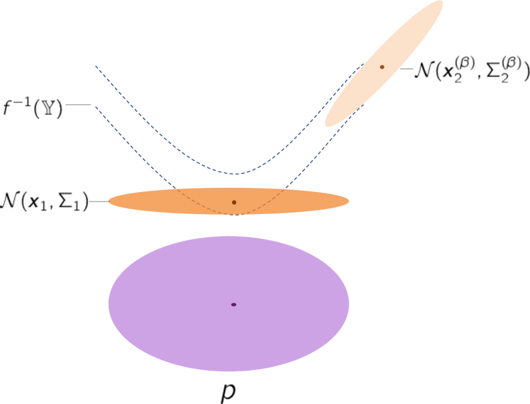
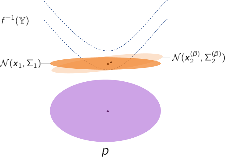
The scale parameter $\beta$ controls the relative tradeoff between the repulsive and the attractive potentials, and consequently, the spacing between $\bm{x}_{k}$ and the fixed centers $\bm{x}_{\mathrm{fixed}}^{(1)},\ldots,\bm{x}_{\mathrm{fixed}}^{(n_{\mathrm{fixed}})}$. To see this, imagine that the system contains a single fixed charge at $\bm{x}_{1}$, and the optimization problem in Equation 5 has been set up to find an appropriate location for a new Gaussian component, whose center will be at $\bm{x}_{2}$ (see Figure 2 for an illustration). If $\beta$ is very small, then the total potential energy will be dominated by electrostatic repulsion and the minimizer of $\mathcal{J}(\bm{x}_{2})$ will be far away from $\bm{x}_{1}$, possibly where $p(\bm{x}_{2})$ is small. On the other hand, if $\beta$ is large, then the pseudo-prior potential energy will dominate and the minimizer will be close to the nearest local minimum of $p(\bm{x})$, preventing exploration of $f^{-1}(\mathbb{Y})$ away from $\bm{x}_{1}$. Both these situations are undesirable, and hence, $\beta$ must be chosen suitably. However, a suitable value of $\beta$ isn’t known a priori. To ensure a spacing that’s appropriate for the purposes of importance sampling, A-BIMC employs a continuation scheme to implicitly fix $\beta$, which is described next.

Parameter continuation

The basic idea behind the continuation scheme in A-BIMC is the following. The scheme tries several values of $\beta$ to minimize Equation 5, creates prospective IS mixtures corresponding to each minimizer, and then selects one that is most appropriate (in a sense that will be made precise shortly).

At the beginning of Stage-1, the minimum and maximum values for $\beta$, $\beta_{\min}$ and $\beta_{\max}$, are computed by studying the relative magnitudes of $\mathcal{U}(\bm{x})$ and $\mathcal{P}(\bm{x})$. Then, the scheme tries five different values of $\beta$, logarithmically spaced between $\beta_{\min}$ and $\beta_{\max}$, starting at $\beta_{\min}$. Each value of $\beta$ leads to a solution of the optimization problem in Equation 5, say $\bm{x}_{k}^{(\beta)}$. Through Equations 3 and 4 each minimizer $\bm{x}_{k}^{(\beta)}$ is in turn associated with a new prospective component $\mathcal{N}(\bm{x}_{k}^{(\beta)},\bm{\Sigma}_{k}^{(\beta)})$, which can be added to the IS mixture with weight $\alpha_{k}^{(\beta)}$ leading to a prospective IS mixture, say $Q_{k}^{(\beta)}$. To decide whether $Q^{(\beta)}_{k}$ is suitable or not, the scheme computes a sample estimate of the KL divergence $D_{\mathrm{KL}}(Q_{k-1}||Q_{k}^{(\beta)})$ between the current IS mixture $Q_{k-1}$ and $Q_{k}^{(\beta)}$. The scheme tries larger and larger values of $\beta$ as long as $D_{\mathrm{KL}}(Q_{k-1}||Q_{k}^{(\beta)})$ increases with $\beta$. If from one iteration to the next, $D_{\mathrm{KL}}(Q_{k-1}||Q_{k}^{(\beta)})$ decreases, the scheme stops and appends the prospective mixture $Q_{k}^{(\beta)}$ from the previous iteration. Hence, implicitly, the scheme selects that value of $\beta$ which makes the resulting IS mixture most different from the current one.

As there’s no guarantee that the minimizer at a given $\beta$, $\bm{x}_{k}^{(\beta)}$, will get accepted, Equation 5 is solved inexactly for each value of $\beta$. Further, the minimizer at some $\beta$, $\bm{x}_{k}^{(\beta)}$, is supplied as the initial guess for solving Equation 5 at the next value of $\beta$. Each $\bm{x}_{k}^{(\beta)}$ is also added to the set of fixed charges, $\bm{\chi}_{\mathrm{fixed}}$, ensuring that any future center is placed away from all $\bm{x}_{k}^{(\beta)}$, in addition to the center that was finally appended to the IS mixture. This prevents A-BIMC from exploring regions that it has previously explored and forces it to venture into previously unexplored regions.

The next paragraph describes how Equation 5 is solved at a given value of $\beta$.

(a) Small $\beta$

(b) Large $\beta$

Figure 2: Illustration of the effect of the scale parameter $\beta$. A small value of $\beta$ leads to the new component with center $\bm{x}_{2}$ being placed far away from $p(\bm{x})$. On the other hand, if $\beta$ is too large, then the new component center will be undesirably close to $\bm{x}_{1}$. The continuation procedure described in Algorithm 1 is designed to yield an intermediate value of $\beta$ that avoids both extremes.

Solving the constrained optimization problem

For a given value of $\beta$, the nonlinearly constrained optimization is solved as follows. First, Equation 5 is transformed to an unconstrained optimization problem via the Augmented Lagrangian (AL) method. In the AL method, the equality constraint is enforced by augmenting the Lagrangian with a term that penalizes violation of the constraint. For Equation 5, choosing a quadratic penalty term yields the following objective function:

(6) $$\mathcal{L}(\bm{x})=\mathcal{U}(\bm{x})+\mathcal{P}(\bm{x})+\frac{1}{2\delta}\left(y-f(\bm{x})\right)^{2}-\lambda\left(y-f(\bm{x})\right)$$

In a traditional implementation of the AL algorithm, the constraint is enforced by solving a sequence of optimization problems where the coefficient of the penalty term, $1/\delta$ and the Lagrange multiplier term, $\lambda$ are modified simultaneously. Eventually, the minimizer of the unconstrained Augmented Lagrangian converges to the minimizer of the constrained optimization problem (see [8] for a basic implementation of this algorithm). Although A-BIMC adopts the AL approach, for the purposes of IS, enforcing $y=f(\bm{x})$ exactly is unnecessary. It suffices if $f(\bm{x})\in\mathbb{Y}$. Starting from some initial guess for $\delta$ and $\lambda$, $\delta_{0},\lambda_{0}$, the algorithm adopts the iterative approach only if the corresponding minimizer, $\bm{x}^{*}$, does not evaluate inside $\mathbb{Y}$. The moment $f(\bm{x}^{*})\in\mathbb{Y}$, the AL iterations are terminated.

Procedure 1 Continuation

1:current IS mixture $Q_{k-1}$, set of fixed charges $\bm{\chi}_{\mathrm{fixed}}$, set of values for the continuation parameter $B=\{\beta_{1},\beta_{2},\ldots,\beta_{|B|}\}$, initial guess for the quadratic penalty parameter $\delta_{\mathrm{start}}$, initial guess for the Lagrange multiplier $\lambda_{\mathrm{start}}$, constraint value $y$,

2:IS mixture enriched with a new component $Q_{k}$, new fixed charges discovered $\bm{\chi}_{\mathrm{new}}$, sample estimate of ${D}_{\mathrm{KL}}(Q_{k-1}||Q_{k})$

3:$\bm{\chi}_{\mathrm{new}}\leftarrow\varnothing$

4:Choose $\bm{x}_{\mathrm{start}}\in\mathbb{R}^{m}$

5:for $1\leq j\leq|B|$ do

6:    Using $\delta_{\mathrm{start}},\lambda_{\mathrm{start}},\bm{x}_{\mathrm{start}}$ as starting guesses for $\delta,\lambda,\bm{x}$, $\beta=\beta_{j}$ and $\bm{\chi}_{\mathrm{fixed}}$ as the set of fixed charges,

7:     follow Algorithm 2 to minimize Equation 5

8:     $\bm{x}_{\mathrm{new}}\leftarrow\textsc{ModifiedAugmentedLagrangian}(y,\mathbb{Y},\lambda_{\mathrm{start}},\delta_{\mathrm{start}},\bm{x}_{\mathrm{start}})$

9:    Using $\bm{x}=\bm{x}_{\mathrm{new}}$ in LABEL:supplement_optimal_noise_var compute a suitable value of the pseudo-likelihood variance $\sigma_{\mathrm{new}}$

10:    Using $\bm{x}=\bm{x}_{\mathrm{new}},\sigma=\sigma_{\mathrm{new}}$ in Equation 3, compute $\mathbf{H}_{\mathrm{GN}}^{-1}$ and assign it to $\bm{\Sigma}_{\mathrm{new}}$

11:    Obtain a prospective IS distribution $Q_{k}^{(\beta_{j})}$ by adding $\mathcal{N}(\bm{x}_{\mathrm{new}},\bm{\Sigma}_{\mathrm{new}})$ to $Q_{k-1}$

12:    $\bm{x}_{\mathrm{start}}\leftarrow\bm{x}_{\mathrm{new}}$

13:    $\bm{\chi}_{\mathrm{new}}\leftarrow\bm{\chi}_{\mathrm{new}}\cup\{\bm{x}_{\mathrm{new}}\}$

14:    Compute a sample estimate of $D_{\mathrm{KL}}(Q_{k-1}||Q_{k}^{(\beta_{j})})$ and assign it to $\hat{D}_{\mathrm{KL}}[j]$

15:    if $\hat{D}_{\mathrm{KL}}[j]>\hat{D}_{\mathrm{KL}}[j-1]$ then

16:         Try a larger value of $\beta$

17:        continue

18:    else

19:         $Q_{k}^{(\beta_{j-1})}$ was more different from $Q_{k-1}$ than $Q_{k}^{(\beta_{j})}$

20:        $Q_{k}\leftarrow Q_{k}^{(\beta_{j-1})}$

21:        return $(Q_{k},\bm{\chi}_{\mathrm{new}},\hat{D}_{\mathrm{KL}}[j-1])$

22:    end if

23:end for

24:$\hat{D}_{\mathrm{KL}}(Q_{k-1}||Q_{k}^{(\beta_{j})})$ increases with $j$, hence $Q_{k}^{(\beta_{|B|})}$ is most different from $Q_{k-1}$

25:$Q_{k}\leftarrow Q_{k}^{(\beta_{|B|})}$

26:return $(Q_{k},\bm{\chi}_{\mathrm{new}},\hat{D}_{\mathrm{KL}}[|B|])$

This concludes the description of how A-BIMC finds centers of new components. The continuation and modified Augmented Lagrangian algorithms described above are reproduced in pseudo-code in Algorithms 1 and 2. The next subsection describes the termination criterion employed in Stage-1.

Procedure 2 ModifiedAugmentedLagrangian

1:desired constraint value $y$, target interval $\mathbb{Y}$, starting guess for Lagrange multiplier $\lambda_{\mathrm{start}}$, starting guess for penalty coefficient $\delta_{\mathrm{start}}$, starting guess for the optimizer $\bm{x}_{\mathrm{start}}$

2:Approximate minimizer of Equation 5 $\bm{x}^{*}$

3:$\delta\leftarrow\delta_{\mathrm{start}}$

4:$\lambda\leftarrow\lambda_{\mathrm{start}}$

5:$\bm{x}^{*}\leftarrow\bm{x}_{\mathrm{start}}$

6:while $f(\bm{x}^{*})\not\in\mathbb{Y}$ do

7:    Starting from $\bm{x}_{\mathrm{start}}$, compute the approximate minimizer of $\mathcal{L}(\cdot;\delta,\lambda)$ and assign it to $\bm{x}^{*}$

8:    $\lambda\leftarrow\lambda-\frac{1}{\delta}\left(y-f(\bm{x}^{*})\right)$

9:    $\delta\leftarrow 0.5\delta$

10:    $\bm{x}_{\mathrm{start}}\leftarrow\bm{x}^{*}$

11:end while

12:return $\bm{x}^{*}$

3.1.4 Termination

The procedure described above adds new components to the IS mixture in every iteration. Hence, the number of components in the mixture grows steadily. In order to decide whether the IS mixture is sufficiently stable, or conversely, if more components are required, the algorithm keeps track of how the IS mixture changes across iterations. The change in the IS mixture is measured in terms of a quantity that resembles perplexity, $\zeta=\exp(-D_{\mathrm{KL}}(Q_{k-1}||Q_{k}))$, where $Q_{k}$ is the IS mixture at the $k$-th iteration. Since $D_{\mathrm{KL}}\left(Q_{k-1}||Q_{k}\right)\geq 0$, $\zeta\in(0,1]$. The KL divergence here is once again a sample estimate, and is in fact the same quantity computed in the continuation scheme. Stage-1 is terminated if relative change in $\zeta$ falls below a user specified relative change threshold, or its absolute value exceeds a user-specified absolute change threshold.

3.1.5 Summary

In summary, Stage-1 adaptively explores the pre-image of the interval $f^{-1}(\mathbb{Y})$, and yields an IS distribution with the following form:

(7) $$Q(\bm{x})=\sum_{k=1}^{K}\alpha_{k}\mathcal{N}\left(\bm{x}_{k},\bm{\Sigma}_{k}\right).$$

The centers of the Gaussian mixture components are obtained by solving a sequence of optimization problems, the weights $\alpha_{k}$ are heuristically evaluated, and the covariances $\bm{\Sigma}_{k}$ are local Gauss-Newton Hessians. This procedure is heuristic, with no guarantees on the quality of the final Gaussian mixture for importance sampling. Hence, Stage-2 of A-BIMC further modifies the Gaussian mixture that results at the end of Stage-1. Details of Stage-2 are provided next.

3.2 Stage-2

Stage-2 of A-BIMC modifies the Gaussian mixture obtained at the end of Stage-1 via the Mixture Population Monte Carlo algorithm. This subsection begins with a brief introduction to the MPMC algorithm, before describing how it’s employed within A-BIMC.

3.2.1 Mixture Population Monte Carlo method

The MPMC algorithm generates an importance sampling distribution to approximate some target distribution $\pi$ using the following approach. Among all possible Gaussian mixtures with $K$ components, it seeks that mixture $Q^{*}$ which is closest in KL divergence to $\pi$:

(8) $$Q^{*}=\operatorname*{arg\,min}_{Q\in\mathcal{Q}_{K}}D_{KL}(\pi||Q),$$

where $\mathcal{Q}_{K}$ denotes the family of $K$-component Gaussian mixtures. Here, $K$ is assumed to be known and fixed. Importance sampling is then performed using $Q^{*}$.

Seeking $Q^{*}$ is equivalent to seeking its $K$ mixture weights $(\omega_{1}^{*},\ldots,\omega_{K}^{*})$ and the means $\bm{m}_{k}^{*}$ and covariances $\mathbf{C}_{k}^{*}$ of its components. Equation 8 can be restated as:

(9) $$(\omega_{1}^{*},\ldots,\omega_{K}^{*},\bm{m}_{1}^{*},\ldots,\bm{m}_{K}^{*},\mathbf{C}_{1}^{*},\ldots,\mathbf{C}_{K}^{*})=\operatorname*{arg\,min}_{\begin{subarray}{c}\sum_{k}\omega_{k}=1\\ \mathbf{C}_{k}\succ\bm{0}\\ \bm{m}_{k}\in\mathbb{R}^{m}\end{subarray}}D_{\mathrm{KL}}\left(\pi||\sum_{k}\omega_{k}\mathcal{N}(\bm{m}_{k},\mathbf{C}_{k})\right),$$

which, from the definition of KL divergence, is equivalent to

(10) $$(\omega_{1}^{*},\ldots,\omega_{K}^{*},\bm{m}_{1}^{*},\ldots,\bm{m}_{K}^{*},\mathbf{C}_{1}^{*},\ldots,\mathbf{C}_{K}^{*})=\operatorname*{arg\,max}_{\begin{subarray}{c}\sum_{k}\omega_{k}=1\\ \mathbf{C}_{k}\succ\bm{0}\\ \bm{m}_{i}\in\mathbb{R}^{m}\end{subarray}}\int\pi(\bm{x})\log\left(\sum_{k}\omega_{k}\mathcal{N}(\bm{m}_{k},\mathbf{C}_{k})\right)\mathrm{d}\bm{x}.$$

Here, the notation $\mathbf{C}_{k}\succ\bm{0}$ implies that $\mathbf{C}_{k}$ is positive definite. The constraints $\sum_{k}\omega_{k}=1$ and $\mathbf{C}_{k}\succ\bm{0}$ are necessary for $Q^{*}$ to remain a valid Gaussian mixture.

The optimization problem in Equation 10 strongly resembles maximum likelihood estimation of the mixture parameters, for which the Expectation Maximization (EM) algorithm [6] is usually employed. As a result, MPMC also closely follows the EM algorithm, except that the sum over i.i.d. data is replaced with an integration over $\pi(\bm{x})$. Like EM, MPMC is an iterative algorithm. Starting from some initial mixture, the mixture weights, and the means and covariances of its components are updated in every iteration. The update expressions involve evaluating expectations with respect to $\pi$. These integrals are in turn evaluated using autonormalized importance sampling, and hence, the algorithm only requires the ability to evaluate $\pi(\bm{x})$ up to a constant.

The progress of the algorithm is tracked by measuring the normalized perplexity of the IS weights used in computing the update integrals. The algorithm is terminated when, at some iteration, the normalized perplexity stagnates, or becomes sufficiently close to 1. The Gaussian mixture obtained at the end of this iterative procedure is then used for importance sampling of $\pi$. The next subsection describes how MPMC is used within A-BIMC.

3.2.2 MPMC and A-BIMC

As the mixture obtained at the end of Stage-1, $Q_{K}$, only roughly approximates $q^{*}$, it is further refined using the MPMC algorithm. One way to do this could be to set the target distribution $\pi$ to $q^{*}$, and supplying $Q_{K}$ as the initial guess to the algorithm. However, this would require additional evaluations of $f$, driving up the computational cost of the method. A-BIMC instead constructs a cheap surrogate for $f$, denoted $f_{\mathrm{surrogate}}$, and then sets $\pi(\bm{x})=1_{\mathbb{Y}}(f_{\mathrm{surrogate}}(\bm{x}))p(\bm{x})$ in order to tune $Q_{K}$. The surrogate $f_{\mathrm{surrogate}}$ is constructed as follows.

Procedure 3 ForwardSurrogate

1:input-output map $f(\cdot)$, set of fixed charges $\bm{\chi}_{\mathrm{fixed}}$, query location $\bm{x}$

2:A surrogate $f_{\mathrm{surrogate}}(\bm{x})$ for $f(\bm{x})$

3:Find that member of $\bm{\chi}_{\mathrm{fixed}}$ to which $\bm{x}$ is closest and assign it to $\bm{x}_{{\min}}$

4:$f_{\mathrm{surrogate}}(\bm{x})\leftarrow f(\bm{x}_{{\min}})+\nabla f(\bm{x}_{{\min}})^{T}(\bm{x}-\bm{x}_{{\min}})+0.5(\bm{x}-\bm{x}_{{\min}})^{T}\nabla^{2}f(\bm{x}_{{\min}})(\bm{x}-\bm{x}_{{\min}})$

5:return $f_{\mathrm{surrogate}}(\bm{x})$

During the continuation phase in Stage-1, A-BIMC saves $(f(\bm{x}_{\mathrm{fixed}}^{i}),\nabla f(\bm{x}_{\mathrm{fixed}}^{i}),\nabla^{2}f(\bm{x}_{\mathrm{fixed}}^{i}))$ at each fixed charge $\bm{x}_{\mathrm{fixed}}^{i}$. These three quantities can be used to construct a second-order Taylor series expansion around each fixed charge $\bm{x}_{\mathrm{fixed}}^{i}$. In order to approximate $f(\bm{x})$ at some $\bm{x}$, the surrogate first finds the fixed charged in $\bm{\chi}_{\mathrm{fixed}}$ which is closest in Euclidean distance to $\bm{x}$, let’s say $\bm{x}_{\min}$. Then, $f(\bm{x})$ is approximated as: $f(\bm{x}_{\min})+\nabla_{\bm{x}}f(\bm{x}_{{\min}})^{T}(\bm{x}-\bm{x}_{{\min}})+0.5(\bm{x}-\bm{x}_{{\min}})^{T}\nabla_{\bm{x}}^{2}f(\bm{x}_{{\min}})(\bm{x}-\bm{x}_{{\min}})$. Pseudo-code for this procedure is provided in Algorithm 3.

The surrogate constructed here is merely a suggestion. If a better, more principled surrogate is available, then that may be used in constructing the target distribution $\pi$ in MPMC. Irrespective of how the surrogate is constructed, it is only used while tuning $Q_{K}$ via MPMC and nowhere else. The actual function $f$ is used for the final importance sampling stage. This concludes the presentation of the A-BIMC methodology. The next subsection offers a summary of our algorithm.

3.3 Summary

In summary, our algorithm involves the following steps:

• Constructing the IS distribution: First, the importance sampling distribution is constructed. This itself is a two stage process. In Stage-1, a sequence of optimization problems is solved to adaptively discover $f^{-1}(\mathbb{Y})$. The resulting sequence of local minima are consolidated into a Gaussian mixture using heuristic estimates of the covariance and mixture weights. Stage-2 involves tuning the Gaussian mixture that results from the first stage against $q^{*}(\bm{x})$ via MPMC. This involves evaluations of $q^{*}(\bm{x})$, which in turn requires evaluations of $f(\bm{x})$. While tuning with MPMC, a cheap surrogate for $f$ is used, in order to keep function evaluations low. For simplicity, we will denote the importance sampling mixture at the end of this two stage procedure using just $Q$.

• Sampling the IS distribution: Finally, the mixture that is obtained at the end of the previous stage is used as an importance sampling density to evaluate the rare-event probability. In this step, A-BIMC uses true evaluations of $f(\bm{x})$, instead of any surrogates.

Pseudo-code for the A-BIMC methodology is provided in Algorithm 4.

Procedure 4 AdaptiveBIMC

1:input-output map $f(\cdot)$, target interval $\mathbb{Y}$, mean $\bm{x}_{0}$ and covariance $\bm{\Sigma}_{0}$ of $p(\bm{x})$, absolute and relative tolerances $\epsilon_{\mathrm{abs}}$ and $\epsilon_{\mathrm{rel}}$, number of samples $N$

2:importance sampling estimate of the rare event probability $\tilde{\mu}^{N}$, the associated relative root mean square error $\tilde{e}_{\mathrm{RMS}}^{N}$

3:

4:Construct the IS distribution

5:Stage-1

6:Find $\bm{x}_{\mathrm{start}}$ such that $f(\bm{x}_{\mathrm{start}})\in\mathbb{Y}$

7:Linearize $f(\bm{x})$ around $\bm{x}_{\mathrm{start}}$, and use this linearized approximation in Equation (SM7) in [13] to compute the optimum pseudo-likelihood variance ${\sigma^{*}}^{2}$ and optimum pseudo-data $y^{*}$

8:Construct the pseudo-posterior $p(\bm{x}|y)$ using $y=y^{*}$ and $\sigma=\sigma^{*}$ and compute its MAP point, assign it to $\bm{x}_{\mathrm{MAP}}$

9:Using $\bm{x}=\bm{x}_{\mathrm{MAP}},\sigma=\sigma^{*}$ in Equation 3, compute $\mathbf{H}_{\mathrm{GN}}^{-1}$ and assign it to $\bm{\Sigma}_{\mathrm{MAP}}$

10:$Q_{1}\leftarrow\mathcal{N}(\bm{x}_{\mathrm{MAP}},\bm{\Sigma}_{\mathrm{MAP}})$

11:$\bm{\chi}_{\mathrm{fixed}}\leftarrow\{\bm{x}_{\mathrm{MAP}}\}$

12:Choose initial guess for the Lagrange multiplier $\lambda_{\mathrm{start}}\in\mathbb{R}$

13:Choose initial guess for the penalty $\delta_{\mathrm{start}}\in\mathbb{R}^{+}$

14:Choose values for the scale parameter $B\leftarrow\{\beta_{1},\beta_{2},\ldots,\beta_{|B|}\}$.

15:for $k=2,3,\ldots$ do

16:    Sample $y$ uniformly from $\mathbb{Y}$

17:    Add a new component to $Q_{k-1}$ using Algorithm 1. As a side effect, obtain $\hat{D}_{\mathrm{KL}}(Q_{k-1}||Q_{k})$ and $\bm{\chi}_{\mathrm{new}}$

18:     $(Q_{k},\bm{\chi}_{\mathrm{new}},\hat{D}_{\mathrm{KL}})\leftarrow\textsc{Continuation}(Q_{k-1},\delta_{\mathrm{start}},\lambda_{\mathrm{start}},y,\bm{\chi}_{\mathrm{fixed}},B)$

19:    $\bm{\chi}_{\mathrm{fixed}}\leftarrow\bm{\chi}_{\mathrm{fixed}}\cup\bm{\chi}_{\mathrm{new}}$

20:    $\zeta[k]\leftarrow\exp(-\hat{D}_{\mathrm{KL}}(Q_{k-1}||Q_{k}))$

21:    if $\zeta[k]>\epsilon_{\mathrm{abs}}$ or $|\zeta[k]-\zeta[k-1]|/\zeta[k]<\epsilon_{\mathrm{rel}}$ then break

22:    end if

23:end for

24:Assume Stage-1 required ${K}$ iterations. Denote the mixture obtained ${Q_{K}}$.

25:

26:Stage-2

27:Using $\bm{\chi}=\bm{\chi}_{\mathrm{fixed}}$, employ Algorithm 3 to construct a surrogate $f_{\mathrm{surrogate}}$ for $f$.

28:Define $q^{*}_{\mathrm{surrogate}}\propto\bm{\mathrm{1}}_{\mathbb{Y}}(f_{\mathrm{surrogate}})p$.

29:Tune the IS mixture $Q_{K}$ to match $q^{*}_{\mathrm{surrogate}}$ using the MPMC algorithm, and assign the tuned mixture to $Q$

30:

31:Compute the rare event probability

32:Generate $N$ samples from the tuned mixture $\bm{X}_{1},\ldots,\bm{X}_{N}\overset{\mathrm{i.i.d.}}{\sim}Q$

33:$w_{i}\leftarrow\frac{\bm{\mathrm{1}}_{\mathbb{Y}}(f(\bm{X}_{i}))p(\bm{X}_{i})}{Q(\bm{X}_{i})},i=1,\ldots,N$

34:$\tilde{\mu}^{N}\leftarrow\frac{1}{N}\sum_{i}w_{i}$

35:$\tilde{e}^{N}_{\mathrm{RMS}}\leftarrow\sqrt{\sum_{i}(w_{i}-\tilde{\mu}^{N})^{2}}/N\tilde{\mu}^{N}$

36:return $\tilde{\mu}^{N},\tilde{e}_{\mathrm{RMS}}^{N}$

4 Experiments

This section presents results from a variety of numerical experiments. These experiments have been designed to assess how A-BIMC performs, expose the conditions that affect its performance, and in the process, unearth any potential limitations. To provide a context in which the results can be understood, the following remarks are in order.

Measuring performance

Objectively assessing the performance of an IS scheme solely from samples is still an unresolved question. Appealing to Chebyshev’s inequality [12] reveals a simple (but potentially restrictive) criterion: a low relative RMSE is sufficient for $\tilde{\mu}^{N}$ to be close to $\mu$ with high probability. As a diagnostic quantity, the relative RMSE also appears in disguise elsewhere; for instance, as the $\chi^{2}$-divergence between $q^{*}$ and $Q$ in [10, 1], the Effective Sample Size [9, 1, 10] or the second moment of the IS weights [1]. These studies have established the central role that the relative RMSE and its variants play in controlling the error between $\tilde{\mu}^{N}$ and $\mu$. For this reason, A-BIMC’s performance is primarily measured in terms of the relative RMSE. Since the true relative RMSE is unavailable, it is approximated via samples. Let $\bm{X}_{1},\ldots,\bm{X}_{N}\overset{i.i.d.}{\sim}Q(\bm{x})$ be $N$ samples from $Q$. The relative RMSE, defined in Equation (4) in Part I, can be estimated via samples as follows:

$$\tilde{e}_{\mathrm{RMS}}^{N} =\sqrt{\frac{\sum_{i}w_{i}^{2}}{\left(\sum_{i}w_{i}\right)^{2}}-\frac{1}{N}}$$

where $w_{i}=\bm{\mathrm{1}}_{\mathbb{Y}}(f(\bm{X}_{i}))p(\bm{X}_{i})/Q(\bm{X}_{i})$. The sample estimate of the relative RMSE has been shown to be an inadequate indicator of performance in [3]. However, in the large $N$ asymptotic regime, $\tilde{e}_{\mathrm{RMS}}^{N}$ approximates $e_{\mathrm{RMS}}$ well, and therefore $\tilde{e}_{\mathrm{RMS}}$ and its variants are expected to perform adequately as diagnostics [1]. In addition to the sample estimate of the relative RMSE, the ESS is also reported. Taking inspiration from the the function-specific ESS defined in [9], the following rare-event specific ESS is employed:

$$\mathrm{ESS}=\frac{1}{\sum_{i}\bar{w}_{i}^{2}},$$

where $\bar{w}_{i}=\bm{\mathrm{1}}_{\mathbb{Y}}(f(\bm{x}_{i}))p(\bm{x}_{i})/Q(\bm{x}_{i})/\sum_{j}\bm{\mathrm{1}}_{\mathbb{Y}}(f(\bm{x}_{j}))p(\bm{x}_{j})/Q(\bm{x}_{j})$. LABEL:supplement:relationship_erms_ess establishes that there exists a one-to-one correspondence between $\tilde{e}_{\mathrm{RMS}}^{N}$ and the rare-event specific ESS. Hence, the ESS is only reported for a few representative experiments.

Measuring function evaluations

Along with performance estimates, the number of function evaluations required during Stage-1 of A-BIMC are also reported. Recall that Stage-1 solves a sequence of optimization problems to iteratively explore $f^{-1}(\mathbb{Y})$. Here, it is assumed that A-BIMC has access to an oracle who, when queried, returns $f(\bm{x}),\nabla f(\bm{x})$ and $\nabla^{2}f(\bm{x})$ at some $\bm{x}$. The function evaluations reported correspond to the number of queries that Stage-1 made to this oracle. It is further assumed that the cost of evaluating the surrogate $f_{\mathrm{surrogate}}$ during Stage-2 is negligible, and is not reported.

Forward maps

As proof-of-concept, the toy periodic map presented in Section 2 is revisited. In addition, A-BIMC is tested on synthetic maps drawn from the following classes of functions. Maps that belong to these classes are sufficiently rich to expose both the advantages and drawbacks of A-BIMC. The manner in which these maps are actually constructed is detailed while describing the setup for each experiment. The function classes are:

• Quadratic polynomials: The class of functions $f:\mathbb{R}^{m}\rightarrow\mathbb{R}$ of the form: $f(\bm{x})=\bm{x}^{T}\mathbf{H}\bm{x}+\bm{b}^{T}\bm{x}+c$ for some $\mathbf{H}\in\mathbb{R}^{m\times m}$, $\bm{b}\in\mathbb{R}^{m}$ and $c\in\mathbb{R}$. In other words, $f$ is nonlinear but with constant curvature. Note that for this class of functions, $f=f_{\mathrm{surrogate}}$.

• Cubic polynomials: The class of functions $f:\mathbb{R}^{m}\rightarrow\mathbb{R}$ of the form: $f(\bm{x})=\bm{\mathcal{S}}:\bm{\mathcal{X}}+\bm{x}^{T}\mathbf{H}\bm{x}+\bm{b}^{T}\bm{x}+c$ for some $\bm{\mathcal{S}}\in\mathbb{R}^{m\times m\times m}$, $\mathbf{H}\in\mathbb{R}^{m\times m}$, $\bm{b}\in\mathbb{R}^{m}$ and $c\in\mathbb{R}$ and where the tensor contraction $\bm{\mathcal{S}}:\bm{\mathcal{X}}$ is defined as $\bm{\mathcal{S}}:\bm{\mathcal{X}}=\mathcal{S}_{ijk}x_{i}x_{j}x_{k}$. Now, $f$ is nonlinear and again possesses varying curvature since $\nabla^{2}f(\bm{x})$ varies with $\bm{x}$.

Implementation

A-BIMC has been implemented in MATLAB. The optimization problems posed in Section 3.1.3 are solved using the Trust Region algorithm, as implemented in MATLAB’s in-built fminunc routine. In the implementation, the gradients and the Hessian of the objective function are passed to the optimizer. Because each individual optimization problem the continuation phase of Stage-1 does not need to be solved exactly, the optimizer is terminated if the gradient is reduced by a factor of $10^{-2}$ or if the number of iterations exceeds 5.

Algorithmic parameters

Unless otherwise noted, A-BIMC is run using the following parameters: $\epsilon_{\mathrm{abs}}=1-10^{-3}$ and $\epsilon_{\mathrm{rel}}=10^{-3}$. For Stage-2, the specific variant of MPMC used is termed the Rao-Blackwellized version in [2]. By default, MPMC uses $N_{\mathrm{MPMC}}=10^{6}$ samples per iteration and a maximum of 50 iterations.

The following subsections present the results of numerical experiments. The first experiment is a proof-of-concept that establishes whether all of BIMC’s drawbacks have been rectified. The next experiment subjects A-BIMC to problems of increasing dimensionality. This is followed by a study of its performance as the rarity of the problem is increased.

(a) Samples

(b) Relative RMSE versus number of samples $N$

Figure 3: A comparison of simple Monte Carlo, BIMC, and the various stages of A-BIMC using the toy problem - samples (Figure 3(a)) and relative error (Figure 3(b)). Figure 3(a) shows 5000 samples from $q^{*}$ and 500 from each estimator. While the IS mixture at the end of Stage-1 of A-BIMC is an improvement over BIMC, tuning via MPMC drastically improves its quality.

4.1 A toy problem

Purpose

This is a proof-of-concept experiment whose aim is to establish that A-BIMC leads to a consistent importance sampling distribution and that all of the drawbacks listed in Section 2 have been fixed.

Setup

As noted earlier, for this toy problem, the forward map is defined as $f(\bm{x}):=\sin(x_{1})\cos(x_{2})$. The nominal distribution is $p(\bm{x})=\mathcal{N}(\bm{x}_{0},\bm{\Sigma}_{0})$ where $\bm{x}_{0}=[0,1]^{T}$ and $\bm{\Sigma}_{0}=0.3\mathbf{I}_{2}$. A Monte Carlo simulation using $10^{6}$ samples results in the following 99% confidence interval: $3.413\times 10^{-2}\pm 4.68\times 10^{-4}$.

Results and discussion

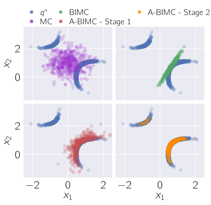
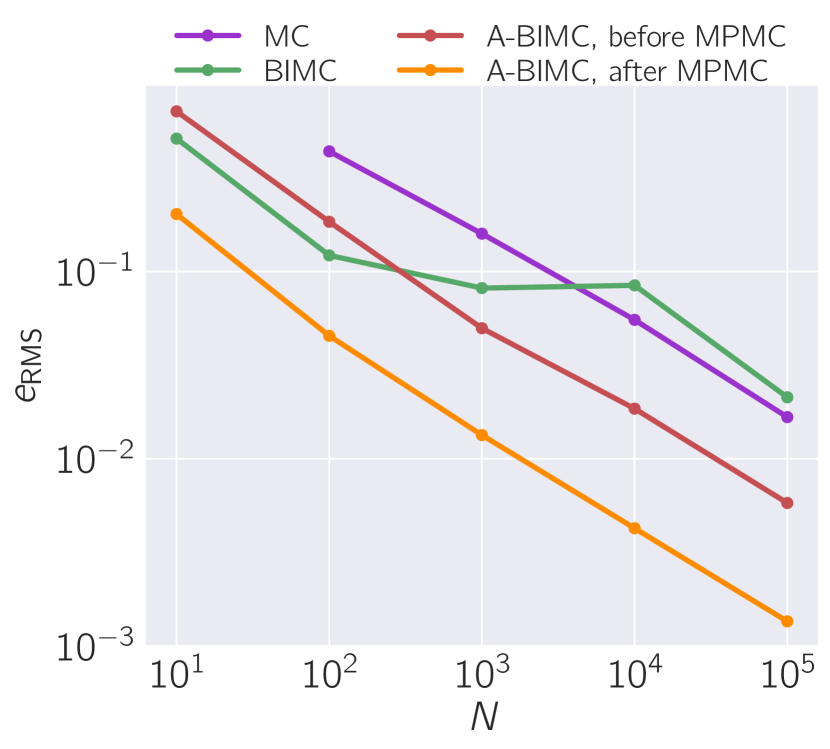
Figure 3 compares the quality of various estimators - MC, BIMC, and A-BIMC at the end of Stages 1 and 2, in terms of the quality of samples and the relative RMSE. As is evident, Stage-1 yields a mixture that roughly approximates $q^{*}$. This mixture contains 46 components. MPMC takes this rough approximation of $q^{*}$ and and tunes it so that it better resembles $q^{*}$. Also noteworthy is the fact that at the end of Stage-1, A-BIMC finds the successfully finds the secondary mode of $q^{*}$, albeit with an insufficient mixture weight, a discrepancy which is fixed by MPMC. The total number of function evaluations required by A-BIMC was 3051.

4.2 Effect of dimensionality

Purpose

Importance sampling schemes are known to suffer from the curse of dimensionality. This experiment investigates how increasing the dimensionality of the rare-event probability estimation problem affects A-BIMC’s performance.

Setup

To obtain a complete understanding of A-BIMC’s performance, two different notions of dimensionality are varied. The first notion of dimensionality is the ambient dimension of the problem, which is simply the dimension of the space in which the uncertain parameters live. Therefore, if $\bm{x}\in\mathbb{R}^{m}$, then the ambient dimension of the problem is $m$. The second notion of dimension is that of the intrinsic dimension $m_{\mathrm{int}}$ of the problem. The intrinsic dimension of the posed rare-event probability estimation problem is defined to be the dimension of the subspace in which the ideal importance sampling distribution $q^{*}$ differs from the nominal distribution $p$. Such a situation can arise, for instance, if the forward map $f$ is sensitive only to a few directions in the input parameter space. This definition of intrinsic dimension for rare-events closely follows that for Bayesian inference, where it is taken to be the dimension of the subspace where the posterior differs from the prior [11, 5].

Given the ambient dimension $m$, the intrinsic dimension of the problem is specified as follows. First, $p$ is set to $p=\mathcal{N}(\bm{1}_{m},\mathbf{I}_{m})$, where $\bm{1}_{m}=[1,1,\ldots 1]^{T}\in\mathbb{R}^{m}$ is the vector of all 1’s and $\mathbf{I}_{m}$ is the $m\times m$ identity matrix. Then forward maps $f(\bm{x})$ are constructed so that they satisfy $\partial f/\partial x_{i}=0$ for $i=m_{\mathrm{int}}+1,\ldots,m$. This way, the maps are insensitive to any variation of the input parameters in $\text{span}\{\bm{e}_{m_{\mathrm{int}}+1},\ldots,\bm{e}_{m}\}$, where $\bm{e}_{i}$ is the $i$-th canonical basis vector. In addition, since $p$ is a Normal distribution with identity covariance, $q^{*}$ differs from $p$ only in span$\{\bm{e}_{1},\ldots,\bm{e}_{m_{\mathrm{int}}}\}$. In span$\{\bm{e}_{m_{\mathrm{int}+1}},\ldots,e_{m}\}$, $q^{*}$ is identical to $p$ by construction.

As for actually constructing $\bm{\mathcal{S}},\mathbf{H},\bm{b}$, the following procedure is adopted. Given $m_{\mathrm{int}}$ and $m$, we set (in MATLAB notation) $\bm{\mathcal{S}}[m_{\mathrm{int}}+1:m,m_{\mathrm{int}}+1:m,m_{\mathrm{int}}+1:m]=\mathbf{0}$, $\mathbf{H}[m_{\mathrm{int}}+1:m,m_{\mathrm{int}}+1:m]=\mathbf{0}$ and $\bm{b}[m_{\mathrm{int}}+1:m]=\bm{0}$. Now, let $\bar{\bm{\mathcal{S}}}$, $\bar{\mathbf{H}}$ and $\bar{\bm{b}}$ denote the non-zero blocks of $\bm{\mathcal{S}}$, $\mathbf{H}$, and $\bm{b}$, i.e., $\bm{\mathcal{S}}[1:m_{\mathrm{int}},1:m_{\mathrm{int}},1:m_{\mathrm{int}}],\mathbf{H}[1:m_{\mathrm{int}},1:m_{\mathrm{int}}],\bm{b}[1:m_{\mathrm{int}}]$. These are constructed as follows.

The tensor $\bar{\bm{\mathcal{S}}}$ is constructed as: $\bar{\bm{\mathcal{S}}}=10\bm{\mathcal{I}}+\bm{\mathcal{G}}$. Here $\bm{\mathcal{I}}$ is defined as $\bm{\mathcal{I}}_{ijk}:=\bm{\delta}_{ij}\bm{1}_{k}$, $\bm{\delta}_{ij}$ is the Kronecker delta, and $\bm{1}_{k}$ assumes the value 1 for all possible $k$. The tensor $\bm{\mathcal{G}}$ is a tensor of i.i.d. standard Normal variables, $\bm{\mathcal{G}}_{ijk}\sim\mathcal{N}(0,1)$. The matrix $\bar{\mathbf{H}}$ is constructed as a sample from a Wishart distribution with scale matrix $2\mathbf{I}_{m_{\mathrm{int}}}$ and $m_{\mathrm{int}}+1$ degrees of freedom, $\bar{\mathbf{H}}\sim W(2\mathbf{I}_{m_{\mathrm{int}}},m_{\mathrm{int}}+1)$. The vector $\bar{\bm{b}}$ is a vector of uniformly distributed random numbers in $[0,1]$, $\bar{\bm{b}}_{i}\sim\mathbb{U}({[0,1]})$.

The ambient dimension $m$ is set to $16,32,64$, and for $m$, the intrinsic dimension $m_{\mathrm{int}}$ is varied from a minimum of $m_{\mathrm{int}}=4$ to a maximum of $m_{\mathrm{int}}=m$.

Results and discussion

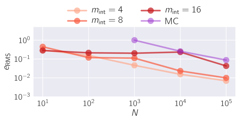
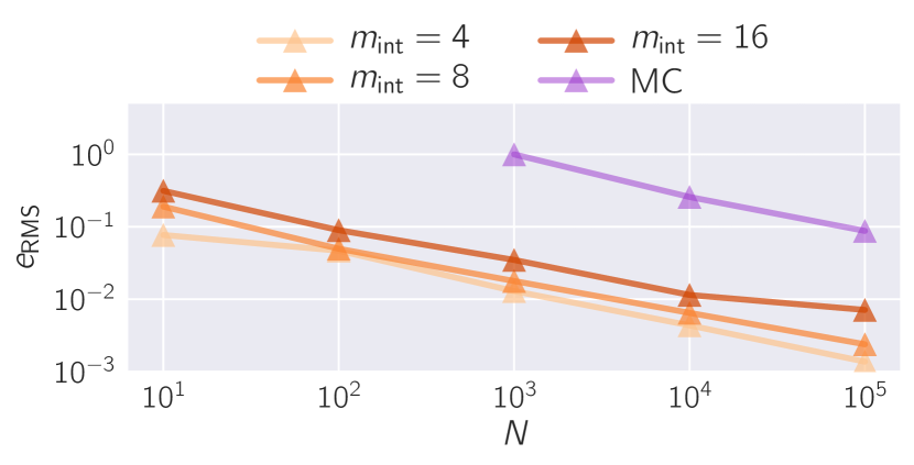
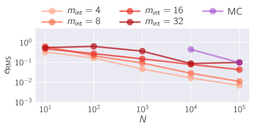
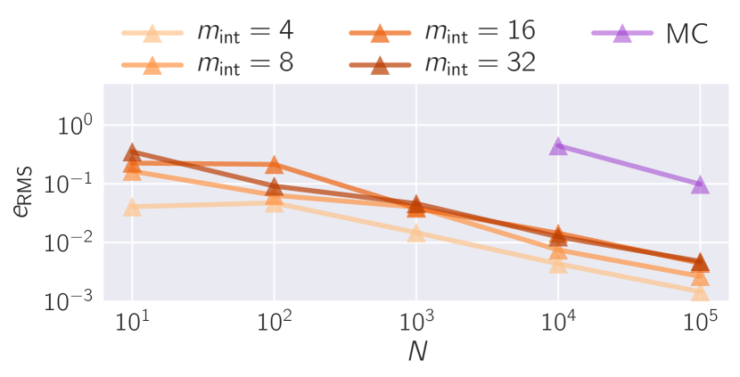
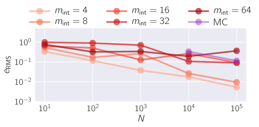
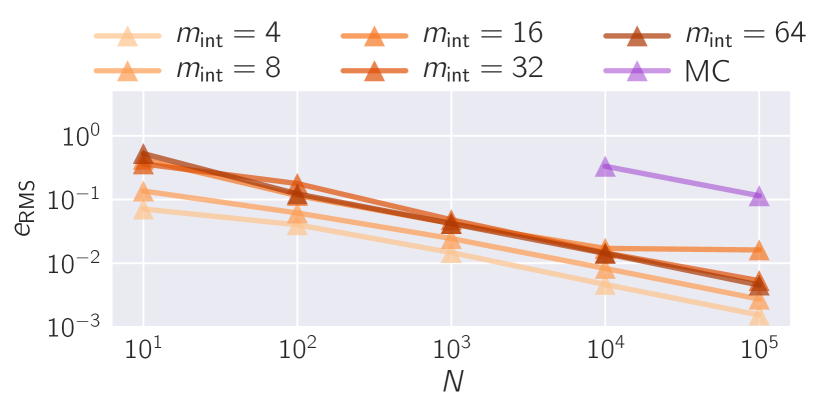
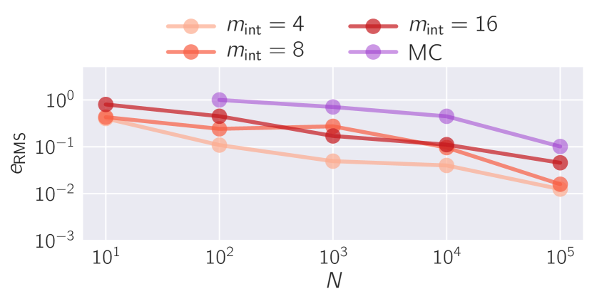
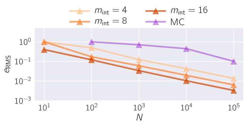
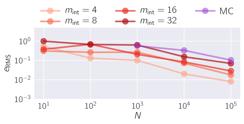
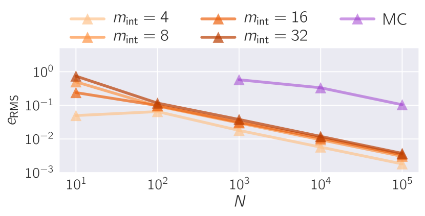
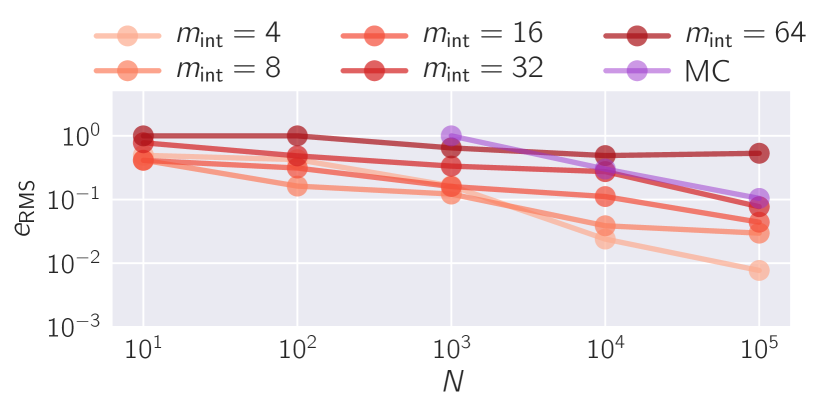
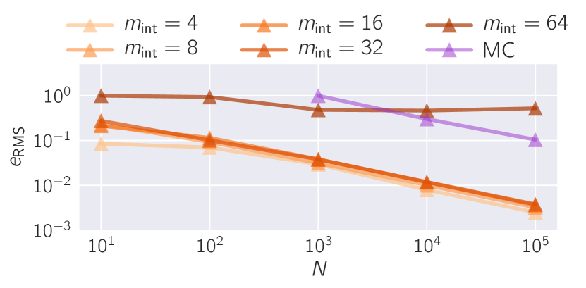
Figures 4 and 5 reports the relative RMSE obtained. Stage-1 of A-BIMC only yields consistent estimates of the rare-event probability at low $m_{\mathrm{int}}$. At large $m_{\mathrm{int}}$, the error after Stage-1 fails to exhibit the expected $1/\sqrt{N}$ convergence. Stage-2 of A-BIMC appears weakly dependent on the intrinsic dimension of the problem. Notably, it consistently leads to low errors. For instance, achieving a relative RMSE of around $10\%$ only requires $N=100$ samples. Exceptions to this trend is the cubic case at $m_{\mathrm{int}}=4$ and $m=16$ and $m_{\mathrm{int}}=64,m=64$.

The poor performance at $m_{\mathrm{int}}=4$ and $m=64$ (this case is referred to as F1 subsequently) can be attributed to the surrogate $f_{\mathrm{surrogate}}$ not possessing sufficient accuracy. The poor performance at $m_{\mathrm{int}}=m=64$ (referred to as F2 subsequently) is due to the relatively higher ambient dimensionality of the problem, which causes MPMC to result in mixtures whose components have rank-deficient covariance matrices. These limitations, as well as a measures to diagnose and fix them, are discussed in Section 5.

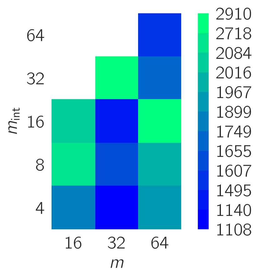
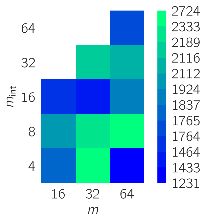
Figure 6 reports the number of function evaluations required by Stage-1 of A-BIMC. The function evaluations display no significant trend with either ambient, or the intrinsic dimension of the problem. Tables 2 and 3 reports the best and worst observed normalized-ESS, $\mathrm{ESS}/N$ for each ambient dimension at $N=10^{4}$. The normalized-ESS reflects the poorly performing cases noted earlier ($\{m_{\mathrm{int}}=4,m=16\}$ and $\{m_{\mathrm{int}}=64,m=64\}$. The actual rare-event probabilities are reported in LABEL:supplement:additional_results.

(a) Stage-1, $m=16$

(b) Stage-2, $m=16$

(c) Stage-1, $m=32$

(d) Stage-2, $m=32$

(e) Stage-1, $m=64$

(f) Stage-2, $m=64$

Figure 4: Convergence of the relative RMSE, $e_{\mathrm{RMS}}$, with number of samples $N$ at various combinations of $m$ and $m_{\mathrm{int}}$ for the quadratic problem.

$m$	Worst ESS (corresponding $m_{\mathrm{int}}$)	Best ESS (corresponding $m_{\mathrm{int}})$
16	0.43 (16)	0.84 (4)
32	0.32 (16)	0.84 (4)
64	0.25 (16)	0.82 (4)

Table 2: Worst and best observed normalized-ESS at various ambient dimension $m$ for the quadratic problem. The normalized-ESS is reported at $N=10^{4}$. The values in parentheses indicate the intrinsic dimension $m_{\mathrm{int}}$ at which the normalized-ESS was observed.

(a) Stage-1, $m=16$

(b) Stage-2, $m=16$

(c) Stage-1, $m=32$

(d) Stage-2, $m=32$

(e) Stage-1, $m=64$

(f) Stage-2, $m=64$

Figure 5: Convergence of the relative RMSE, $e_{\mathrm{RMS}}$, with number of samples $N$ at various combinations of $m$ and $m_{\mathrm{int}}$ for the cubic problem.

$m$	Worst ESS (corresponding $m_{\mathrm{int}}$)	Best ESS (corresponding $m_{\mathrm{int}})$
16	0.051 (4)	0.48 (16)
32	0.41 (32)	0.75 (32)
64	0.00046 (64)	0.61 (4)

Table 3: Worst and best observed normalized-ESS at various ambient dimension $m$ for the cubic problem. The normalized-ESS is reported at $N=10^{4}$. The values in parentheses indicate the intrinsic dimension $m_{\mathrm{int}}$ at which the normalized-ESS was observed.

(a) Quadratic problem

(b) Cubic problem

Figure 6: Function evaluations required by Stage-1 of A-BIMC display no significant trend with either $m$ or $m_{\mathrm{int}}$.

4.3 Effect of rarity

Purpose

This experiment is designed to answer the following question: how does A-BIMC perform as the magnitude of the rare-event probability is decreased?

Setup

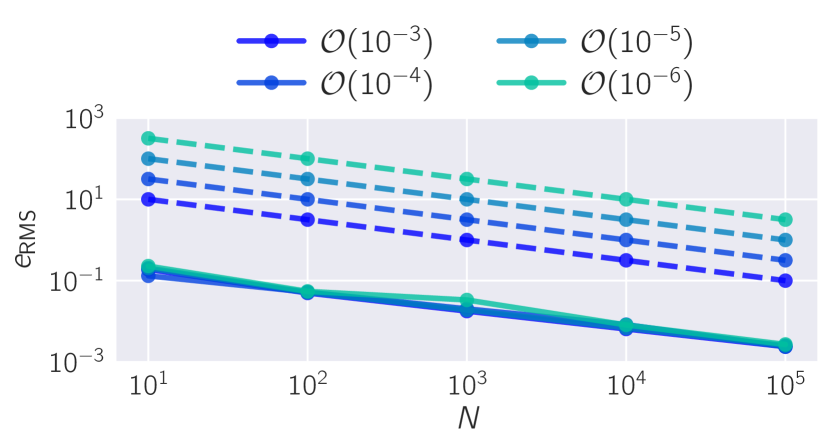
Both the quadratic and cubic forward maps are constructed as in Section 4.2 but the dimensionality of the problem is fixed at $m=16$ and $m_{\mathrm{int}}=8$ so that the effect of decreasing probability level can be extracted. The nominal distribution for both forward maps is also as in Section 4.2, $p(\bm{x})=\mathcal{N}(\mathbf{1},\bm{I}_{m})$. The rarity level is increased by choosing $\mathbb{Y}$ so that the rare-event probability is approximately $\mathcal{O}(10^{-4}),\mathcal{O}(10^{-5}),\mathcal{O}(10^{-6})$ respectively for each forward map.

Results and discussion

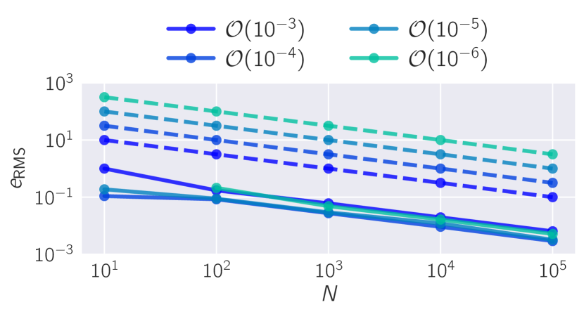
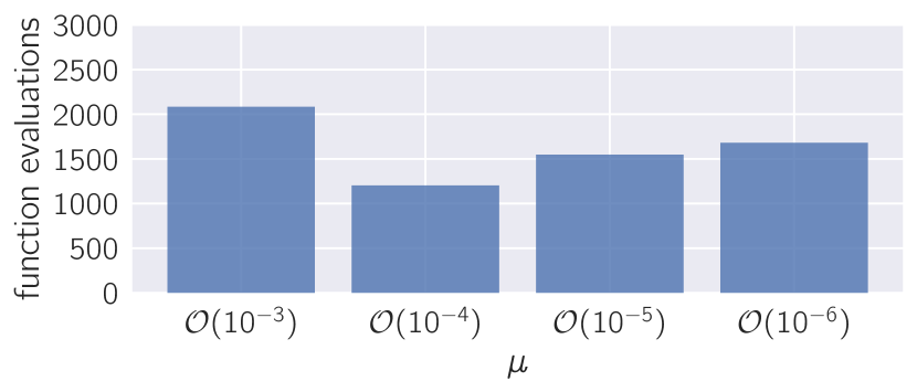
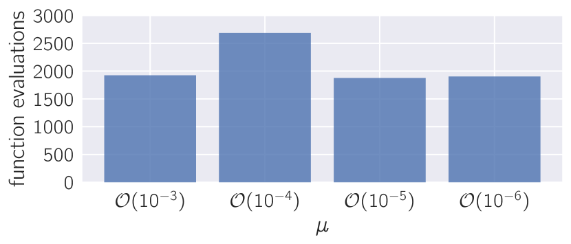
As was demonstrated in Section 2.1 of part 1, the number of samples required by a simple Monte Carlo method to achieve a specified accuracy in the rare-event probability increases as the probability decreases. Figure 7 offers evidence that this is not the case for A-BIMC. Figure 8 demonstrates that the number of function evaluations required to explore $f^{-1}(\mathbb{Y})$ also remains approximately constant as the probability magnitude decreases.

(a) Quadratic problem

(b) Cubic problem

Figure 7: This figure demonstrates that A-BIMC (solid lines) performs consistently well even as the magnitude of the rare-event probability is decreased from $\mathcal{O}(10^{-3})$ to $\mathcal{O}(10^{-6})$. The dashed lines show the expected theoretical performance of the simple Monte Carlo estimator $\hat{\mu}$, computed using the expression $\sqrt{(1-\hat{\mu})/(\hat{\mu}N)}$ (see Section 2.1 of Part I).

(a) Quadratic problem

(b) Cubic problem

Figure 8: Function evaluations required by A-BIMC remain independent of the magnitude of the rare-event probability, as this probability is decreased from $\mathcal{O}(10^{-3})$ down to $\mathcal{O}(10^{-6})$.

This concludes the presentation of results of numerical experiments. The next section explores how A-BIMC can fail, and in particular, offers explanations for why A-BIMC performed unsatisfactorily in experiments F1 and F2 in Section 4.2.

5 Failure

In this section, we explore how A-BIMC can fail. A-BIMC’s failure is tied to inappropriately choosing the tolerance ${\epsilon}_{\mathrm{abs}}$, or the number of samples used by MPMC per iteration, $N_{\mathrm{MPMC}}$ (in order to keep the number of tunable parameters to a minimum, we always choose $\epsilon_{\mathrm{rel}}=1-\epsilon_{\mathrm{abs}}$). Hence, this section doubles as a discussion on the consequences of choosing these parameters inappropriately. In addition to exploring the mechanisms behind failure, recommendations for diagnosing, as well as mitigating it, are offered.

Inappropriate $\epsilon_{\mathrm{abs}}$

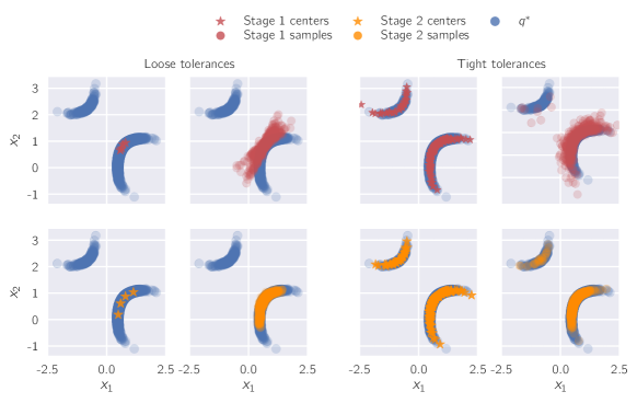
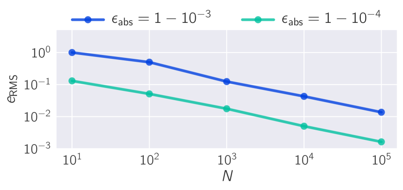
Recall that $\epsilon_{\mathrm{abs}}$ is a tolerance on how similar mixtures are allowed to be from one iteration to the next in Stage-1. A smaller value of $\epsilon_{\mathrm{abs}}$ means mixtures are allowed to be similar, which in turn implies more components will be added to the mixture in Stage-1. Adding more components is advantageous for two reasons - it aids discovery of disjoint regions of $f^{-1}(\mathbb{Y})$, and leads to a more accurate surrogate $f_{\mathrm{surrogate}}$ (this fact illustrated in Figure 9 for the toy problem). At the same time, adding more components requires solving more optimization problems, driving up the computational cost of Stage-1. Clearly, $\epsilon_{\mathrm{abs}}$ represents trade-off between a smaller computational footprint and better discovery of $f^{-1}(\mathbb{Y})$. However, an a priori prescription for $\epsilon_{\mathrm{abs}}$ remains elusive at this time.

A possible hypothesis for why A-BIMC performed poorly in experiment F1 is that $\epsilon_{\mathrm{abs}}=1-10^{-3}$ was too loose, leading to an inaccurate surrogate. Running A-BIMC at $\epsilon_{\mathrm{abs}}=1-10^{-4}$ immediately improves the surrogate, and consequently, A-BIMC’s performance, lending credibility to this hypothesis (see Figure 10(a)). Therefore, an inappropriate $\epsilon_{\mathrm{abs}}$ can be diagnosed by a low ESS. Note that A-BIMC need not be re-run from scratch to correct for loose $\epsilon_{\mathrm{abs}}$. Let $Q_{1}^{\mathrm{loose}}$ and $\bm{\chi}^{\mathrm{loose}}_{\mathrm{fixed}}$ denote the IS mixture and set of fixed charges computed at the end of Stage-1 with a loose $\epsilon_{\mathrm{abs}}$. Then, rectifying the effect of a loose $\epsilon_{\mathrm{abs}}$ simply involves starting from $Q_{1}^{\mathrm{loose}}$ and $\bm{\chi}_{\mathrm{fixed}}^{\mathrm{loose}}$ and re-running lines 10-17 of Algorithm 4 using a tighter $\epsilon_{\mathrm{abs}}$. This will have the same effect as a cold restart of A-BIMC using the tighter tolerance.

Figure 9: This figure illustrates the effect of varying the tolerances $\epsilon_{\mathrm{abs}}$ and $\epsilon_{\mathrm{rel}}$. The left half of the figure corresponds to a loose tolerance, $\epsilon_{\mathrm{abs}}=1-10^{-1}$, while the right half corresponds to a tighter tolerance, $\epsilon_{\mathrm{abs}}=1-10^{-5}$. In both cases, $\epsilon_{\mathrm{rel}}=1-\epsilon_{\mathrm{abs}}$ and $N_{\mathrm{MPMC}}=10^{6}$. Tighter tolerances lead to a greater number of components in the mixture and can aid the discovery of disjoint regions of $f^{-1}(\mathbb{Y})$. However, they increase the computational cost. For instance, $\epsilon_{\mathrm{abs}}=1-10^{-1}$ required 266 function evaluations, whereas $\epsilon_{\mathrm{abs}}=10^{-5}$ required 19749. All cases show 5000 samples from $q^{*}$ and 500 samples from the IS mixture obtained after Stages 1 and 2.

(a) Failure case F1 is remedied by increasing $\epsilon_{\mathrm{abs}}$.

(b) Failure case F2 is remedied by increasing $N_{\mathrm{MPMC}}$.

Figure 10: Fixing failure cases F1 and F2. Decreasing $\epsilon_{\mathrm{abs}}$ in failure case F1 increased the number of function calls from 1765 to 3429.

High ambient dimensionality

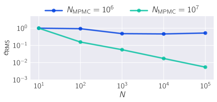
MPMC is particularly susceptible to failure when the dimension of the parameter $\bm{x}$ is high. This is because the update formulae for $\alpha_{k}$’s, $\bm{x}_{k}$’s and $\bm{\Sigma}_{k}$’s in MPMC are posed as high-dimensional integrals. These integrals are approximated via IS, and at a given sample size, become poorer and poorer approximations of the the true updates as the dimension of the parameters increases. This failure mechanism usually manifests as one of the $\bm{\Sigma}_{k}$’s becoming rank-deficient during the tuning procedure. This is the mechanism of failure in experiment F2. In this case, it is truly the high ambient dimensionality of the problem, and not other factors, such as an inaccurate surrogate, that cause MPMC to fail. This is confirmed in Figure 10(b), where MPMC is rerun using $N_{\mathrm{MPMC}}=10^{7}$, but with the same surrogate. Increasing $N_{\mathrm{MPMC}}$ successfully improves performance. This failure mode usually manifests as a rank-deficient covariance matrix in one of the mixture components during MPMC, and it can be fixed by increasing $N_{\mathrm{MPMC}}$. Note that such a failure mode, compared to an inappropriate $\epsilon_{\mathrm{abs}}$, is relatively benign as it doesn’t require additional evaluations of $f$.

Poor surrogates

The surrogate used to replace full evaluations of $f(\bm{x})$ is a heuristic, and unfortunately, possesses no guarantees as to its accuracy. If the surrogate poorly approximates $f(\bm{x})$, then the resulting mixture will be a poor approximation of $\bm{\mathrm{1}}_{\mathbb{Y}}(f(\bm{x}))$. This failure is tied to item 1, but can also occur independently, for instance when no computationally tractable $\epsilon_{\mathrm{abs}}$ can deliver a surrogate that is accurate enough.

6 Conclusion and future work

In Part II of this article, we extend the applicability of BIMC, an algorithm for computing rare-event probabilities. The extended algorithm, called Adaptive-BIMC, proceeds in two stages. In Stage-1, A-BIMC constructs a rough approximation of the (theoretical) ideal importance sampling distribution by exploring the regions that trigger the rare-event on a global scale. This is in contrast to BIMC, which can only achieve local exploration of the region of interest around the so-called pseudo-MAP point. Global exploration in A-BIMC is achieved by solving a sequence of optimization problems to discover points along the region of interest, and then accruing the discovered points into a Gaussian mixture distribution. Both the optimization, and the covariances of the components in the Gaussian mixture are derivative-aware. Stage 2 of A-BIMC refines the rough approximation yielded by Stage 1 using the Mixture Population Monte Carlo algorithm. While this would usually require further evaluations of the forward map, we avoid doing so by using a heuristic surrogate which is constructed on-the-fly.

Results from several numerical experiments allow us to make the following conclusions:

• A-BIMC is independent of the rarity level of the problem, a trait desirable from any scheme that aims to efficiently compute rare-event probabilities

• A-BIMC does break down as the ambient dimensionality of the problem increases. This breakdown is due to MPMC, the algorithm employed to refine the Gaussian mixture distribution yielded by Stage 1.

We suspect that if the intrinsic dimension of the problem is low, the breakdown with increasing ambient dimension can be arrested. This can be done by performing importance sampling only in the subspace in which the ideal importance sampling density differs from the nominal distribution. The challenge here will be to discover the subspace in question. In the future, we aim to apply techniques developed for dimension reduction in Bayesian inverse problems [16, 4] to reduce the dimension of the rare-event probability estimation problem.

References

- [1] S. Agapiou, O. Papaspiliopoulos, D. Sanz-Alonso, and A. M. Stuart, Importance sampling: Intrinsic dimension and computational cost, Statist. Sci., 32 (2017), pp. 405–431, https://doi.org/10.1214/17-STS611, https://doi.org/10.1214/17-STS611.
- [2] O. Cappé, R. Douc, A. Guillin, J.-M. Marin, and C. P. Robert, Adaptive importance sampling in general mixture classes, Statistics and Computing, 18 (2008), pp. 447–459, https://doi.org/10.1007/s11222-008-9059-x, https://doi.org/10.1007/s11222-008-9059-x.
- [3] S. Chatterjee and P. Diaconis, The sample size required in importance sampling, Ann. Appl. Probab., 28 (2018), pp. 1099–1135, https://doi.org/10.1214/17-AAP1326, https://doi.org/10.1214/17-AAP1326.
- [4] P. G. Constantine, Active subspaces: Emerging ideas for dimension reduction in parameter studies, vol. 2, SIAM, 2015.
- [5] T. Cui, J. Martin, Y. M. Marzouk, A. Solonen, and A. Spantini, Likelihood-informed dimension reduction for nonlinear inverse problems, Inverse Problems, 30 (2014), p. 114015.
- [6] A. P. Dempster, N. M. Laird, and D. B. Rubin, Maximum likelihood from incomplete data via the em algorithm, Journal of the Royal Statistical Society. Series B (Methodological), 39 (1977), pp. 1–38, http://www.jstor.org/stable/2984875.
- [7] P. S. Laplace, Memoir on the probability of the causes of events, Statist. Sci., 1 (1986), pp. 364–378, https://doi.org/10.1214/ss/1177013621, https://doi.org/10.1214/ss/1177013621.
- [8] J. Nocedal and S. Wright, Numerical optimization, Springer Science & Business Media, 2006.
- [9] A. B. Owen, Monte Carlo theory, methods and examples, 2013.
- [10] D. Sanz-Alonso, Importance sampling and necessary sample size: An information theory approach, SIAM/ASA Journal on Uncertainty Quantification, 6 (2018), pp. 867–879, https://doi.org/10.1137/16M1093549, https://doi.org/10.1137/16M1093549, https://arxiv.org/abs/https://doi.org/10.1137/16M1093549.
- [11] A. Spantini, A. Solonen, T. Cui, J. Martin, L. Tenorio, and Y. Marzouk, Optimal low-rank approximations of Bayesian linear inverse problems, SIAM Journal on Scientific Computing, 37 (2015), pp. A2451–A2487.
- [12] R. Vershynin, High-dimensional probability: An introduction with applications in data science, vol. 47, Cambridge University Press, 2018.
- [13] S. Wahal and G. Biros, Supplementary materials: BIMC: The Bayesian Inverse Monte Carlo method for goal oriented uncertainty quantification. Part I.
- [14] S. Wahal and G. Biros, Supplementary materials: BIMC: The Bayesian Inverse Monte Carlo method for goal oriented uncertainty quantification. Part II.
- [15] R. Wong, Academic Press, 1989, https://doi.org/https://doi.org/10.1016/B978-0-12-762535-5.50006-4, http://www.sciencedirect.com/science/article/pii/B9780127625355500064.
- [16] O. Zahm, T. Cui, K. Law, A. Spantini, and Y. Marzouk, Certified dimension reduction in nonlinear bayesian inverse problems, arXiv preprint arXiv:1807.03712, (2018).