SHARP: An Adaptable, Energy-Efficient Accelerator for Recurrent Neural Networks

Abstract

The effectiveness of Recurrent Neural Networks (RNNs) for tasks such as Automatic Speech Recognition has fostered interest in RNN inference acceleration. Due to the recurrent nature and data dependencies of RNN computations, prior work has designed customized architectures specifically tailored to the computation pattern of RNN, getting high computation efficiency for certain chosen model sizes. However, given that the dimensionality of RNNs varies a lot for different tasks, it is crucial to generalize this efficiency to diverse configurations.

In this work, we identify adaptiveness as a key feature that is missing from today’s RNN accelerators. In particular, we first show the problem of low resource-utilization and low adaptiveness for the state-of-the-art RNN implementations on GPU, FPGA and ASIC architectures. To solve these issues, we propose an intelligent tiled-based dispatching mechanism for increasing the adaptiveness of RNN computation, in order to efficiently handle the data dependencies. To do so, we propose Sharp as a hardware accelerator, which pipelines RNN computation using an effective scheduling scheme to hide most of the dependent serialization. Furthermore, Sharp employs dynamic reconfigurable architecture to adapt to the model’s characteristics.

Sharp achieves 2x, 2.8x, and 82x speedups on average, considering different RNN models and resource budgets, compared to the state-of-the-art ASIC, FPGA, and GPU implementations, respectively. Furthermore, we provide significant energy-reduction with respect to the previous solutions, due to the low power dissipation of Sharp (321 GFLOPS/Watt).

Keywords Recurrent Neural Network (RNN), Long-Short-Term Memory (LSTM), Accelerator, Scheduling, Reconfigurability, Low Power

1 Introduction

Recurrent Neural Networks (RNN) represent a well-known Deep Learning (DL) model [1, 2, 3], with increasing popularity for applications that are based on sequence-to-sequence processing  [4, 5, 6, 7], such as speech recognition [8] and machine translation [9]. A key attribute of this class of neural networks is that they use past information to improve model accuracy. Long-Short-Term-Memory (LSTM) [1] and Gated-Recurrent Unit (GRU) are the two most commonly used RNN. They can potentially remember useful information over a long period of time, providing high accuracy. RNNs have shown great effectiveness in many sequence processing problems and have fostered state-of-the-art research innovations, such as in natural language processing tasks, e.g., machine reading comprehension [10, 11, 12] and language modeling [13, 14, 15], and speech recognition [16, 17].

Figure 1: Flop-efficiency of Titan V GPU, performing different real-world sequence processing applications, i.e. Machine Comprehension (MC) [10], Speech Recognition (SR) [8], Language Modeling (LM) [18], and Machine Translation (MT) [19] using cuDNN library [20] and enabling TCUs with mixed-precision.

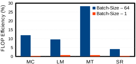
To meet the requirements of real-time inference at large scale, a high-performance and energy efficient accelerator for RNN is highly desired. However, two reasons make it very difficult to accomplish efficient RNN computation by CPUs or GPUs in parallel [21, 22]: (1) recurrent behaviour of RNN architecture which imposes several data-dependencies, (2) limited parallel tasks due to the enforced low batch size by Service-Level Agreements (SLAs) in the inference evaluation [23, 24].

First, RNN has complex dependencies and serialization, which limits the amount of parallelism that can be exploited by many cores. Take the state-of-the-art RNN in cuDNN library [20] on GPU as an example, Figure 1 shows that FLOP efficiency, i.e. the relative FLOPs performance to the peak, for a high-end GPU (Titan V), when running different applications. Note that the evaluation is measured by enabling tensor-core-units (TCUs) using the FP16/FP32 mixed-precision, as explained in [25]. As seen, GPU is extremely under-utilized when performing services of batch size 1. Furthermore, even when using larger batch size of 64, the GPU achieves moderate utilization, between 4% to 28% of peak performance. The reason is that GPU only operates efficiently when there is high level of parallelism available, such as for training. However, for RNN inference, even though the amount of computation (matrix-vector multiplications) increases for long sequences, as in speech recognition or machine translation tasks, the parallelism is limited due to recurrent steps and data dependencies.

Second, for the online inference scenario, queries come in one-by-one and have stringent latency SLA, often in single milliseconds [23, 24]. This requirement further reduces data reuse and available parallelism in RNN inference. Recently, there have been several efforts on either CPU [26], or GPU [23, 22], to improve the efficiency of RNN inference. However, they show poor scalibility for either small or large models with different sequence length.

Because the performance of RNN on general-purpose processors has difficulties to meet the requirements of real-time inference in modern applications, accelerating RNN through either customized architectures [21, 27] or neural processing units (NPU) [24, 28] has been recently explored. These systems are implemented on either ASICs or FPGAs. FPGAs are attractive for their cost and reconfigurability, whereas ASICs are more energy-efficient. However, we show that even though previous accelerators have achieved good performance improvement over CPUs and GPUs, they suffer from two important issues, which are low resource utilization and suboptimal energy consumption. There are two reasons on why existing approaches have low resource utilization: (1) they are efficient only for certain configurations, but they become inefficient when the model configurations start to change; (2) they do not achieve a well-balanced execution pipeline as the available hardware resources increase. Although the two state-of-the-art implementations, Microsoft’s BrainWave [24] and Google’s TPU [28], can achieve high utilization on certain models (e.g. CNNs) and configurations, they only achieve an average utilization of 18% and 3.5% for LSTMs, respectively. We elaborate on the scaling issues of two state-of-the-art ASIC- and FPGA-based RNN accelerators in Section 3.

In this paper, we propose Sharp, an adaptable and energy-efficient architecture for RNN inference acceleration. We show that by carefully analyzing the unique challenge and special characteristics of RNN, we could combine a system-level scheduling scheme and a hardware reconfigurability design to efficiently overcome the data dependencies and low parallelism issue, which yields the most efficient workload-dispatching configuration for each model and addresses the low resource utilization challenges from the previous designs. In particular, we introduce the unfolded scheduling which significantly reduces the length of the RNN critical-path while also strictly overlapping the computations and data transfer time. Furthermore, we introduce dynamic reconfigurability that allows the accelerator to adaptively get high resource utilization for different RNN configurations and handle padding caused by matrixvector multiplication more effectively. Moreover, we show that even though the total power per time unit increases marginally, our design achieves much higher energy-efficiency than existing approaches by making the RNN computations a lot faster.

Figure 2: LSTM computation overview. By looking at the formulas, we see two types of data-dependency, intra-sequence and across sequence, in an LSTM-cell.

Overall, we sum up the paper’s contributions as follows:

• We propose Sharp, a Scalable, High-performance RNN Accelerator, which removes pipeline stalls and resources’ idleness through Reconfiguration and better handles Padding in matrix-vector multiplication.

• We analyze RNN’s critical-path delay, considering its data dependencies, and identify opportunities to hide the latency of sequential parts. We then develop a new scheduling scheme resolving all dependencies.

• To increase the adaptability of our system running different models, we implement a reconfigurable compute-engine that delivers the most efficient resource mapping.

• We conduct thorough evaluation and demonstrate average speedups of 2x, 2.8x, and 82x with respect to the state-of-the-art ASIC, FPGA, and GPU implementations. Furthermore, we obtain 1.7x and 7.4x higher FLOPS/Watt compared to the previous ASIC and FPGA designs, respectively.

The remainder of this paper is organized as follows. Section 2 provides some background on LSTM as an RNN network. Section 3 furthermore introduces some challenges and opportunities regarding RNN acceleration design. Next, we introduce our proposed scheduling technique in Section 5. Afterwards, we describe Sharp’s design in Section 4. Then, Section 6 discusses the architecture’s reconfigurability. We describe the evaluation methodology in Section 7 and show the experimental results in Section 8. Finally, Section 9 reviews some related work, and Section 11 sums up the main conclusions of this work.

2 RNN Background

RNN architectures can simply capture short term dependencies. However, exploiting long term dependencies is challenging and useful at the same time, increasing the quality of the deep-learning models. With this regard, Long-Short-Term-Memory (LSTM) is considered as the most successful and widely used RNN design, with applications in speech recognition [16, 17], machine translation [19] and language modeling [13, 14, 15]. In this section, we explain in detail the structure and behavior of LSTM networks.

An LSTM network is composed of a chain of LSTM cells, and each cell processes two vectors, $x_{t}$ and $h_{t}$ at each time step, corresponding to the input and hidden vectors of the forward and recurrent connections, respectively. It employs four gates in order to recurrently update the cell state and also compute the output. At each recurrent phase, the gates carry out the following actions: the input gate ($i_{t}$) decides how the current input affects the cell-state, while the forget gate ($f_{t}$) removes the amount of useless information from the current cell-state; the cell-update gate ($g_{t}$) modulates the amount of input information that is considered as candidate to update the cell-state; finally, the output gate ($o_{t}$) decides what information to emit from the cell.

Figure 3: BrainWave’s latency and resource-utilization reported in [24], for running different LSTM models.

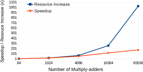
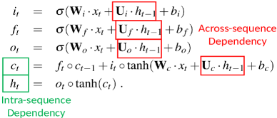
Figure 2 formulates the detailed computation of LSTM at each time step. As depicted, each LSTM gate performs two matrix-vector multiplications (MVMs), which finally decide how to update the cell-state ($c_{t}$), and how to generate the hidden output vector ($h_{t}$) that is recurrently sent to the following time step. Two kinds of dependencies exist in these computations: intra-sequence, since all the gate’s activations must be ready before updating the cell or generating the output; across-sequence, meaning that each step has to wait until its recurrent input is received from the previous time step. Later, we will discuss the parallelism constrains due to the sequential behavior imposed by these dependencies.

3 Challenges and Opportunities

Most of the previous accelerators are designed for a variety of neural networks rather than being tightly optimized for RNNs, specifically LSTM. For instance, NPUs [24, 28] have the parallel multiply-accumulation (MAC) stage as the heart of their pipeline and are not optimized in case the serial part becomes the performance bottleneck for some models. On the other hand, customized accelerators [21, 29] use a relatively small resource budget which therefore causes large delay for MVM, hence overlap the remaining LSTM computation that needs to run sequentially. However, when using more MACs, the issue of efficiently handling LSTM’s dependencies still remains.

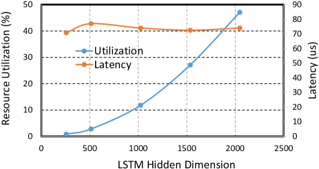
Figure 3 shows the latency and utilization of BrainWave for different LSTM sizes. As the size of the hidden layers decreases, utilization drops drastically, whereas the latency remains the same. However, an efficient design should operate faster as the LSTM workload reduces. The reason for such performance inefficiency is that BrainWave’s pipeline is mainly optimized for some particular large models rather than being adaptable to various models. As stated in [24], for small LSTM, BrainWave’s utilization drops due to two main reasons: (i) the design of large tile dimension for the multiplication units, resulting in wasteful work and resource under-utilization; (ii) the deep pipeline which delays the writing of the dependent data back. In other words, the pipeline is not well-balanced in assigning resources to different stages based on the models’ requirements, which causes many stalls in case one stage is slower.

Figure 4: The figure shows E-PUR’s [21] speedup running EESEN [8], for a range of MAC units. Due to the scalability issue, it does not achieve performance improvement proportional to the increase in resources.

On the other hand, some designs obtain good performance efficiency for a specific model only when resources are limited, but are inefficient with larger resource budgets. For instance, we thoroughly evaluate E-PUR [21], the state-of-the-art dense RNN accelerator, by experimenting across different number of multiply-adder units. Figure 4 shows the performance improvement obtained by increasing resources when accelerating EESEN [8], one of the benchmarks used in [21]. As seen, by raising the multiply-add units above 4K, we are not able to achieve an efficient speedup compared to the increase in the number of resources.

An LSTM cell computes eight different MVMs which can run in parallel at each time step. Previous proposals mainly use vector-vector (VV) [21], vector-matrix (VM) [24] and matrix-matrix (MM) [28] primitives, which are the most simple, straightforward hardware approaches. However, they are less flexible since their vector and matrix dimensions are set to a fixed size, which results in resources’ under-utilization in many cases. In this work, we use vector-scalar (VS) as the basic primitive and implement VV and VM by merging VSs in different dimensions. This way, we can implement resizable primitives by using VSs of different sizes.

To address the aforementioned challenges, we propose SHARP in the next section, as a reconfigurable RNN accelerator design with an efficient pipelining mechanism combined with a new scheduling.

4 SHARP’s Architecture

In this section, we present the architecture of SHARP. First, we describe the accelerator’s pipeline considering LSTM processing flow. Next, we elaborate on each pipeline stages. Finally, we discuss the balance between different component’s latency in order to keep the pipeline fully utilized.

4.1 Overview

Figure 5 illustrates the SHARP’s hierarchical pipelined architecture composed of 3 stages: Compute Unit, Activation MFU (A-MFU), and Cell Updater. Moreover, SHARP uses local FIFOs at all stages in order to control the data-flow and also decouple the producer and consumer pattern as well as computation and memory accesses. Considering LSTM computations, the pipeline performs the following tasks at each time step: First, Compute Unit multiplies the weight matrix and input/hidden vector in a tiled-based fashion, by fetching data from weight and I/H buffers, respectively; Second, after completing each gate’s matrix-vector multiplication (MVM) for both input and hidden vectors, A-MFU runs the activation function, i.e. sigmoid or hyperbolic tangent, on the MVM’s result. Finally, Cell Updater uses all the four gates’ activated results to update the cell-state and produce the hidden outputs for the next step.

Figure 5: The architecture of SHARP accelerator.

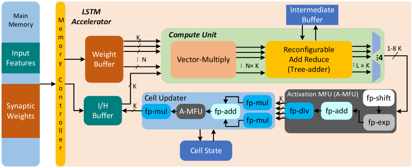
In addition to the functional units, SHARP includes two memory components in order to store the synaptic weight matrices and input and hidden vectors necessary for one RNN layer’s evaluation. This way we can avoid most of the expensive off-chip memory accesses, which is identified as the main feature in most of the state-of-the-art hardware implementations [21, 24, 28]. Regarding the I/H buffer, we use SRAM in order to reduce the access latency and since it often gets modified between sequence processing. Moreover, we model weight buffer as a multi-banked SRAM memory, providing terabytes per second of bandwidth in order to feed the MAC functional unit with maximum throughput. Due to the predictable pattern of RNN computation, we can easily interleave the weight matrices across different memory banks and fully utilize the multiply units without having collisions in accessing similar memory line. Additionally, we use two double-buffered scratchpad memories for storing the cell-state and intermediate results produced between the recurrent time steps.

In the following, we go over the main difference of the SHARP’s design compared to the previous work. Specifically, we will present the reconfigurability for the multiply-add operations and choosing the best tiling dimension for the matrix-multiplication based on the application need and the hardware availability. In the next section, we discuss several scheduling methods and propose one which can tightly couple with SHARP’s pipeline, resulting in both high throughput and low latency compared to the previous designs.

4.2 Resizable MVM Tile-Engine

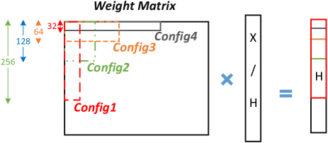
Prior works often use the Dot Product Unit (DPU), which operates on two vectors, to perform MVM by dispatching the weight matrix column-wise [21, 27, 24, 28]. However, we observe that former scheme has to reduce the result-vectors into several outputs which may require 2 reduction levels (such as in [24]). In contrast, we consider row-wise selection for the basic vector operation. Figure 6 (left) shows our Compute Unit structure plus the weight and input and hidden buffers. The Compute Unit is equipped by N K-width vector-scalar (VS) multipliers, each multiplying an input/hidden by k-row elements of the weight matrix and producing N K partial results. The Compute Unit then generates one or multiple vectors of partial sums by accumulating the result-vectors, requiring only 1-level reduction. As depicted by Figure 7, we can allocate the N VS units both row-wise or column-wise, generating resizable MVM tile-engines to go over gate’s computation in a tiled fashion. In the next section, we will show that different choices of K and VS mapping impact performance and utilization of SHARP when running different models.

Figure 6: Vector Multiply plus weight and I/H memory buffers (left) and R-Add-Reduce (right) structure. By using different configurations shown in figure 7, we partition the multiplication outputs and reroute tree-adder’s outputs using four multiplexers accordingly. Based on the selected MVM tiling configuration, we generate 1$k$ to 8$k$ outputs.

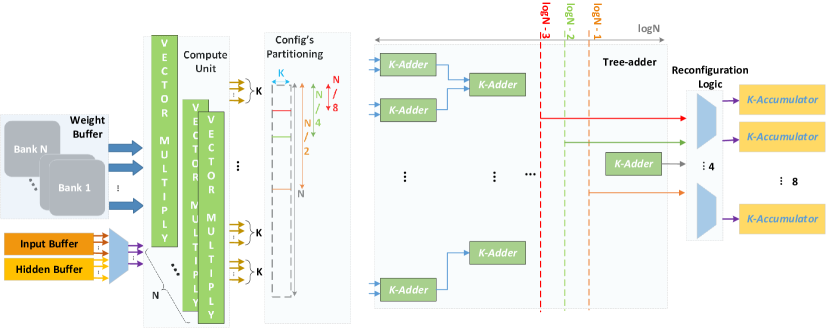
We design Reconfigurable Add Reduce (R-Add-Reduce) using a tree-adder that sums all the $K$-vector results into a $K$ partial sum (Figure 6). This way, we reduce the results in case where all the VS units are mapped column-wise as shown in Config4 of Figure 7. Therefore, R-Add-Reduce has a maximum latency of $log(N)$, when traversing all tree-adder’s levels. In order to hide this delay, we pipeline all the levels of tree, resulting in a 1-cycle add-reduction if the pipeline is full. As Figure 7 depicts, we can update between $1K$ to $8K$ accumulators by choosing the different configurations, as we reach the 4 last levels of tree. Upon completion of each MVM, the accumulators are released for the next phase of the different types of RNN cell’s computation. As the computation of Figure 2 formulates, the input and hidden vectors must be processed before sending out the result from R-Add-Reduce to Activation MFU.

Figure 7: Different MVM configurations chosen based on the $k$-width of the VS units. We consider 32 as the $k$.

4.3 Gate Activation and Cell-Update

Activation MFU is as a configurable multi-functional unit, composed of different arithmetic functions operating several floating-point operations including shift, addition, division, and exponentiation. By combining these units, we implement the two activation functions (sigmoid and hyperbolic tangent) applied to the gate’s outputs. We use the same approach proposed in [21], in order to configure MFU data transfer based on each activation function. For instance, MFU carries out the following actions to get the sigmoid of $X$:

$$X=e^{X}\longrightarrow X=X+1\longrightarrow X=\frac{1}{X}$$ (1)

Based on our synthesis evaluation using Synopsys Design Compiler [30] combined with 32nm technology library, we calculate MFU’s critical-path-delay as 29.14 ns for hyperbolic tangent function. We then partition these operations as shown in Figure 5, to efficiently pipeline them, achieving 1-cycle latency for performing the activation function on each gate’s output.

As soon as all the four gates’ activation results are ready, Cell Updater starts the following two sequential tasks: updating the cell-state, and producing the hidden outputs. Regarding the calculation of cell-state ($c_{t}$), Cell Updater uses the outputs of input, forget and cell-update gates, plus the previous cell-state (see Figure 2). Then, to compute the hidden outputs ($h_{t}$), a hyperbolic tangent is applied to the new cell state, and the result is multiplied by the mask generated from the output gate. Therefore, Cell-Updater also includes an A-MFU plus several point-wise fp16-multiply vector units and a fp32-add vector unit. We pipeline all the operations in order to assure that the calculation of every $\frac{K}{4}$ elements of hidden outputs (combining the 4 gates outputs) finish at each cycle (providing that pipeline is always full).

4.4 Pipeline Efficiency

RNN computation consists of several data dependencies, which makes it a lot challenging to design an efficient pipeline to overlap the independent and the sequential parts. We employ Unfolded scheduler (Section 5) on top of our pipeline design in order to improve performance under different resource configurations. As the MVM operations include an important share of RNN processing, the main focus of previous proposals is to provide more parallelism by increasing MAC resources and reduce RNN latency. However, we observe that for several applications RNN computation can cause a lot of stalls due to its serialization, which limits parallelization. For instance, LSTM models with small dimensions that process long sequences are the most tangible examples that require dealing with lots of dependencies besides the parallel task of MVMs. Thus, we cannot achieve a reasonable performance improvement by only providing high amount of parallelism.

In order to achieve the best throughput, all the pipeline stages should be kept fully utilized. This means that the different components must have similar latency in order for the pipeline to flow without any stalling. Otherwise, it happens that one stage operates faster or slower than others, causing stalls or idleness. This results in under-utilization because of uneven distribution of the amount of work and the number of resources between different stages. In our design, we divide the workload of RNN based on their types of operation, whether they are dependent or independent, and then explore various number of resources for each part. Our experiments show that there is a high correlation between the scheduling scheme and the way pipeline resources are allocated to each part of RNN computation. Furthermore, there is not just one best resource mapping (tiling dimension) to evaluate all the RNN models, since each model has different requirements based on the ratio between parallel and serial tasks. Therefore, by adding some level of reconfigurability at the Compute Unit and R-Add-Reduce components, we increase our design’s adaptability by tailoring the best configuration for each model. We elaborate on the reconfigurability technique in Section 6.

Figure 8: The time-line of LSTM critical-path computation using the four scheduling schemes: a. Sequential, b. Batch, c. Intergate, and d. Unfolded. The $I$, $F$, $G$, and $O$ squares represents the MVM of the Input, Forget, Cell-update, and Output gates, respectively. Red boxes show the matrix batches dispatched to the MVM tile-engine. Long and short arrows show the completion of the whole and a batch of the gate(s), respectively. Moreover, ACC and ACT stands for Accumulate and Activation. We hide the detail for the accumulation and activation of the intermediate gates, since they are overlapped by the MVM tile operations. In order to have equal resources for all the schedules, Intergate and Unfolded techniques take a batch size (for each gate) four and two times smaller than Batch scheduling, respectively.

5 SHARP’s LSTM Schedule

There have been several scheduling approaches proposed in the previous LSTM implementations. These schemes mainly focus on the different processing order of the gates [21, 24] and the input and hidden vectors [29, 26]. However, they result in sub-optimal resource utilization due to inefficiently handling of data dependencies because of not pipelining the whole LSTM. Existing works mainly focus on speeding up MVMs with a high level of parallelism. But according to Amdahl’s Law, overall performance is bounded by the serial execution of the cell-state and hidden units. To overcome this challenge, we propose Unfolded schedule, which removes all the parallelism inefficiencies by strictly overlapping the dependent and independent parts of computation.

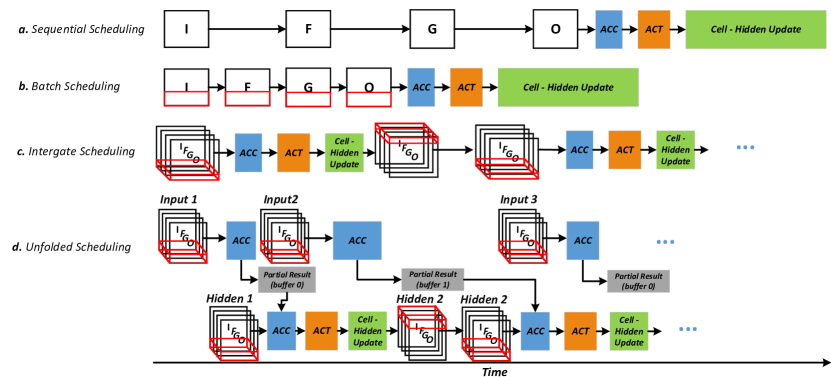
There have been two basic schedulers employed in the previous proposals: Sequential [24, 28, 29] and Intergate [21, 27]. Figures 8.a and 8.c show the two schemes graphically. Sequential scheduling computes the gates in a sequential manner, one gate after another, whereas Intergate scheduling runs all gates’ multiplication together by sharing MAC resources. Although the two techniques have equal latency in processing the gates which includes the MVM and gate activation, there is a slight difference between them. Intergate scheduling can better hide the latency of updating the cell-state and computing the hidden units, by pipelining them with the gates’ computation (output-based tiling). On the other hand, Sequential scheduling has to wait until reaching the last gate (Output) for continuing with the cell-state update and producing hidden units. We will show that the latter schedule outperforms the former in cases that MVM is highly parallelized and operates too fast. However, the challenge is that it makes the serial portion of LSTM computation the main bottleneck.

Figure 8.d depicts the Unfolded technique graphically. As illustrated, we first process the input MVM of each time step and save its result in an intermediate buffer. In other words, we unfold the MVM of the input and hidden vectors in order to hide the serialization delay of the recurrent step $t$ with the input MVM of step $t+1$ (across-sequence dependency), as there is no dependency between the input sequence vectors. Then, after accumulating the hidden MVM’s output with the buffered input results, we can apply the activation function, update the cell-state and generate the hidden outputs. By processing all gates simultaneously, we can overlap the computation of cell-state and hidden units (intra-sequence dependency), by pipelining them in the output-based tiling manner. By using such computation order, we completely overlap the critical-path delay for evaluating LSTM, significantly increasing the utilization rate of parallel MAC resources by hiding the two types of LSTM dependencies shown in Figure 2.

Figure 8 shows the LSTM critical-path time-line, including the gates’ MVMs plus the recurrent serial computation, for the different scheduling methods. In order to go over the gate’s MVM, we divide the weight matrix into several blocks (shown as red boxes) to dispatch to the MVM tile-engine. Critical-path is considered as the longest part of the LSTM computation between recurrent steps. Due to the dependency of the hidden vector, we cannot completely dispatch the next step’s MVM while we are processing last sequential portion of the current step. Sequential scheme pipelines each gate’s computation, including MVM and activation function. Since all the four gates’ outputs must be ready before issuing the cell and hidden update, they run serial to the last gate’s MVM. Batch scheduling is a variant of the previous one, with the difference that it only processes a batch of each gate at a time, allowing to pipeline the whole LSTM computation. By issuing all the gates’ MVMs at the same time for the Intergate approach, we can better overlap the computation and decrease the latency for the cell and hidden update by four times. Our proposal, Unfolded scheduling, not only leverages the advantage of Intergate technique for hiding the intra-sequence dependency, but it also handles the across-sequence dependency. As shown in Figure 8.d, while processing the last sequential computation of the cell-state and hidden outputs for the current time step, the MAC units can still be busy with calculating the next step’s input MVM.

We evaluate Unfolded schedule on GPU and achieve around 20% performance improvement compared to the Sequential scheme. The performance speedup is measured based on the hand-tuned optimized kernels. We observe two sources of inefficiencies for GPU architecture, preventing us from completely exploiting the Unfolded scheduling. First is that the GPU cores require to pay the cost of synchronization to reduce the partial summation across threads, whereas this synchronization is implicit in the SHARP’s architecture by using the tree-based structure. Second, to parallelize the input/hidden GeMM with the sequential part of LSTM computation, we use two streams to launch these kernels. Although, the kernels running on different streams require different hardware resources to do either GeMM (by using Tensor-Cores) or the LSTM-Cell update (through CUDA cores), We find out that the GPU hardware resources cannot be efficiently utilized by the two streams. On the other hand, this approach is more straightforward to the specific SHARP’s acceleration design and through the SHARP’s pipeline, we can tightly tailor the hardware resources to the type of computation. In order to obtain the performance benefits for the Unfolded scheme, we define a new memory layout, which divides the weight matrix into two partitions of input and hidden. Moreover, as we process all the gates together, we put their weights into consecutive parts of the memory based on the tiling dimension selected for MVM processing. We go over the different configurations of the MVM tile-engine in the following section.

A similar approach, introduced by [21, 26], also tries to partition the input and hidden evaluations of LSTM. Their scheme separates the whole input MVMs across all the sequence time-steps, focusing on either improving data locality for accessing weight matrices [21] or optimizing LSTM execution through faster scheduling of GEMMs [26]. In contrast, Unfolded scheduling unfolds the work of each time step individually, and by doing so, we overlap the data-dependency between recurrent serial processing. Therefore, our mechanism introduces a more efficient pipelining for LSTM in order to maximize resource utilization.

6 Improve Adaptability via Reconfigurability

An efficient RNN acceleration design should be able to adapt and scale performance across the space of applications (with different model characteristics) and resource budgets. This means two things: (i) for a fixed resource budget, achieve high-performance execution for different applications (with different model characteristics), and (ii) for a fixed application, scale performance proportionally with resource budget.

In this section, we evaluate SHARP under several configurations for different model characteristics. Then, we will show how the design’s parameters impact the performance of the system regarding various RNN topology. Finally, to improve the adaptability and scalability of our system, we define some level of reconfigurability in order to tailor the tile-engine of SHARP’s architecture to each model.

6.1 Adaptability Issue

Figure 9: Exploration on the $K$-width for the VS units of Compute Unit. The speedups are normalized to 1K-MAC design. In most cases, for different resource budgets, there is not just one configuration providing the best performance for the various LSTM dimensions.

As explained in Section 4.4, MVM operations are the main part of RNN pipeline. Thus, the way they are assigned to the MAC units defines the pipeline efficiency. However, as we observed, there is not just one fixed configuration to dispatch weight matrices to the MVM tile-engine. This is due to two reasons: first, there is always some padding when tiling the matrix MVM; second, there is high performance difference when choosing various tile dimensions for an RNN model. Here, we elaborate more on these adaptability issues and then propose reconfiguration at the MVM tile’s architecture, in order to flexibly adapt to each model’s requirements and achieve the highest performance and utilization.

6.1.1 MVM Padding

By using one multiplication tile-engine to go through the whole MVM of the weight matrix, we incur several padding due to not fitting the last portion of rows and columns of the matrix into a tile. Therefore, this results in some resource under-utilization because of not occupying the multipliers that fall out of the matrix dimension. Furthermore, this padding will continue to exist until multiplying the last column of the matrix. Note that the only case that padding does not exist is when the size of matrix is a multiple of the tile dimension. However, practically speaking, we cannot have as many tile-engines as the different RNN models. In order to handle such inefficiency, we apply reconfiguration in a way that flexibly changes the tile dimension when reaching the last row segment.

6.1.2 Model Diversity

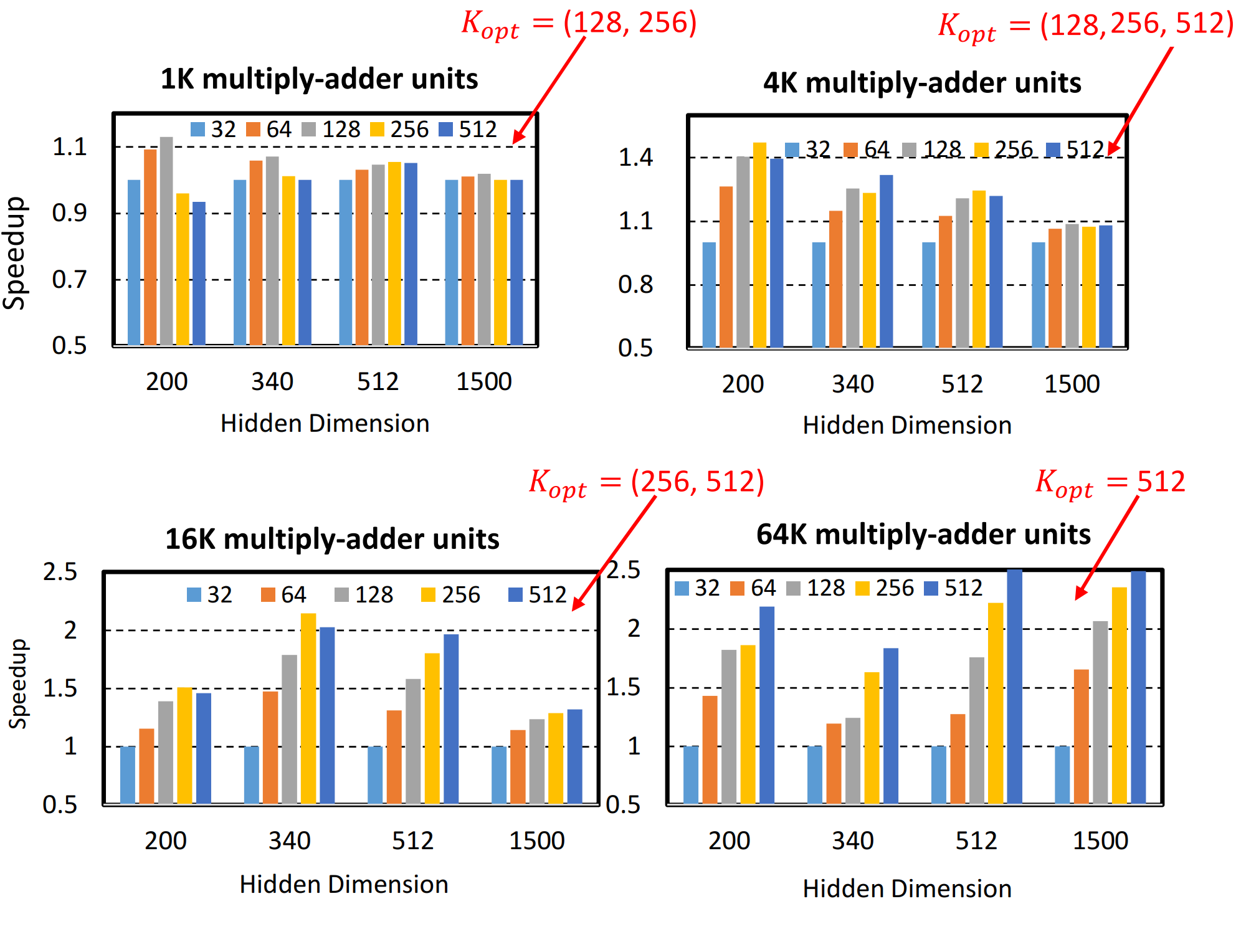
As specified in Section 4.2, Compute Unit is constructed based on a tile with $K$-row and $N$-column multipliers. Considering the same resources, by choosing different $K$ widths, the tile dimension (rows and columns) varies, therefore results in various latency to complete the $K$ partial results of MVM. For instance, if $K$ is too small (Config4 at Figure 7), we place the multipliers more column-wise, producing partial results faster than the case that $k$ is too large(Config1 at Figure 7). Figure 9 shows the $k$-width exploration results in four charts corresponding to 1K, 4K, 16K and 64K multiply-adders, respectively. Each chart illustrates the performance evaluation of choosing several $K$ widths from 32 to 512, regarding the different LSTM hidden dimensions. Note that we assume equal size for both the hidden and input vectors in our experiments. Moreover, we run all the models for the same sequence length of 25 time steps. As seen, there is not just one best configuration for tiling the MVM operations. For instance, in the case of 4K MAC units, there are different optimal $K$-widths (128, 256, and 512) for each LSTM dimension that result in the highest performance speedup.

6.2 Re-configurable Compute Unit

In order to increase the adaptability of our design, we modify the Compute Unit component (as shown in Figure 6) in a way to configure the MVM tile-engine based on each LSTM model dimension. Initially, we consider 32 as the $K$-width of each VS unit. Then, by mapping the VS units at either rows or columns of the weight matrix, we can generate different MVM tiles. Figure 7 depicts the four possible tile configurations of SHARP. Even though the number of multiplications does not differ at each configuration, the data dispatching pattern should match to the row and column selection scheme. This also affects the number of partial results generated by the R-Add-Reduce stage. Therefore, we rearrange the memory organization of the weight matrix by interleaving them based on the configured tile dimension. We also interleave the weights in a way to keep all the VS units uniformly busy.

After delivering the multiplication results to the R-Add-Reduce stage, the tree-adder uses a reconfigurable routing mechanism in order to emit the correct partial results corresponding to the MVM tile configuration. By employing four multiplexers, we support the four configurations shown in Figure 7, by selecting between the outputs of the last four levels of the tree-adder. Figure 6 illustrates the configurations in different colors and also the 4 multiplexers we use to reroute adders’ outputs to match the tiling topology. For example, in the case of Config1 of Figure 7, we select eight partial sums from the fourth last level ($LogN-3$) of the tree-adder to send to the accumulators. Then, by reaching to the end of input and hidden vectors, we will have $8\times K$ MVM results. SHARP’s controller multiplexes based on each model’s specification, by configuring the bit-selects form a table that stores them for the different LSTM dimensions.

6.2.1 Impact on Padding

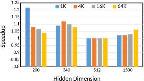
In order to measure the effectiveness of our scheme, we have evaluated padding reconfiguration for the different LSTM models and similar range of resources as for Figure 9. Regarding the MVM tile-engine, we configure $K\_opt$ for each combination of LSTM dimension and MAC resources. Then, we compare the accelerator’s performance for the two cases, applying fixed or reconfigurable configurations. Note that the controller reconfigures the tile-engine dynamically, in a way that $K$ gets as close as to the remaining number of rows. Figure 10 shows the speedups achieved for SHARP by using reconfigurability when running various LSTM models, considering different MAC units. As seen, we improve performance in almost all the cases, except for 512 hidden dimension. The reason is that as 512 is a multiple of $K\_opt$, it causes no padding during MVM tiling, and hence, there is no benefit of reconfiguration. In total, we can get up to 1.22x speedup by applying our approach to alleviate padding.

Figure 10: Performance speedup achieved using the padding reconfiguration technique regarding different resource budgets and for the various LSTM dimensions.

6.2.2 Impact on Adaptability

By using the reconfigurability, we can generate almost all the $K\_opt$ widths for the MVM tile-engine regarding the LSTM models shown in Figure 9, by combining the basic 32-width VS units. We can select between the four options from 32 to 256 for the $K$, achieving most of the performance benefits considering a variety of model dimensions. Note that we explore the configurations offline in order to determine the parameters that reach the best performance for each application. This generates a table with several entries, each storing the optimal configuration for each LSTM’s hidden dimension, including the multiplexing and control-logic applied for the tree-adder. The table is preloaded in an on-chip memory in SHARP, minimizing the cost of reconfiguration both performance- and energy-wise.

Reconfiguration in SHARP has negligible runtime cost and it works as follows. Prior to the execution of each LSTM layer, its optimized architecture’s configuration is fetched from the aforementioned table. Then, SHARP sets the control signals of the multiplexers for the tree-adder accordingly, which has negligible performance overhead. Note that the expensive operations such as experimentally finding the optimal configuration or changing the memory layout are performed offline. Runtime operations only include an access to a small table and setting the control signals of several multiplexers.

For every LSTM network, its weights are rearranged and interleaved offline according to the access-pattern of the optimal configuration. Then, we fetch the memory blocks likewise in order to fill in the on-chip buffers, the SRAM banks corresponding to the VS units. Except for the initial delay to fetch the memory requests (this delay is proportional to the model’s size and the LSTM dimension), we can overlap the rest with the computation of MVM tile-engine. Furthermore, after having the weight matrices reside on-chip, there will be no off-chip memory bottleneck restricting SHARP’s performance. Regarding the input sequences, the I/H buffer (see Figure 4) works in a ping-pong manner. While the MVM tile-engines are processing the current batch of data, SHARP prefetches the next part of input data.

In order to measure the effectiveness of reconfigurability, we compare the configured $K$ against an ideal case of using a hardened $K$ for each model. Our numbers show very similar performance evaluation as all the multiplexing latency is covered by the R-Add-Reduce slack time, imposing no extra cycle to send out the partial sums. The only overhead is for the reconfiguration logic at the controller to select the best configuration, which only happens at the beginning of each LSTM layer’s computation.

By combining the reconfigurability with our scheduling technique, we improve the scalability of our architecture by increasing the performance efficiency with high utilization of the available resources. More specifically, by carefully pipelining the LSTM computation and balancing the latency of pipeline stages, we can overlap most of the data dependencies that limit the parallelism of the MVM operations. Furthermore, comparing with the previous methods that show a poor scaling factor by increasing the number of resources (see Figure 4), we significantly improve the utilization by handling the serialization of LSTM computation more efficiently. For instance, as seen in Figure 9, the speedup numbers are relatively higher in the cases of using more resource budgets such as 16K/64K.

Table 1: SHARP’s configuration.

Technology - Frequency	32 nm - 500 MHz
Weight - I/H Buffer	26 MB - 2.3 MB
Cell State	192 KB
Intermediate Buffer	24 KB
MFUs	64 Units
Multiplication precision	16-bit Floating-Point
Multiply-Adder Units	1K , 4K , 16K , 64K
Peak Bandwidth (GB/s)	11 , 44 , 170 , 561
Peak Throughput(TFLOPs)	0.46 , 1.86 , 7.4 , 29.8

7 Evaluation Methodology

In order to evaluate SHARP, we developed an architectural C++ cycle-accurate simulator to accurately model all the pipeline stages described in Section 4. SHARP’s design is configured using the parameters shown in Table 1. Because we consider different resource budgets from 1K to 64K MACs, we can obtain a range of peak throughput between 0.46 and 29.8 TFLOPS/s. However, by increasing the resources, we require higher peak bandwidth from the on-chip memory components, up to 561 GB/s for the 64K-MAC configuration. To achieve this bandwidth, we increase the banks of SRAM buffers proportional to the VS units of SHARP’s architecture.

In order to estimate the latency, power and area of our design, we implemented all the logic components in Verilog using the Synopsys Design-Ware library [30]. Then, we synthesized them with Synopsys Design Compiler using the commercial 32 nm technology library [31]. For the technology library, we used 0.85 V power configuration and the typical-typical process corner. Furthermore, We modeled the on-chip SRAM buffers in CACTI-P [32] with the same technology parameters. The simulator incorporates the timing of the critical-path-delay from the synthesis results and memory latencies. Finally, to model the off-chip DRAM main memory, we use the Micron Power model for an 8-GB LPDDR [33]. The cycle-accurate simulator provides the activity factor for the different components and the total cycle count, which are used to compute execution time, dynamic and static energy by combining them with the estimations of the Design Compiler, CACTI and Micron power models.

Table 2 shows the area breakdown for the different versions of SHARP. For the 1K-MAC configuration, more than 86% of the area is allocated by the SRAM buffers. However, as we increase the number of MACs, the compute-unit becomes the dominant part of the accelerator’s area. This is because we use half-precision for the multiplication and full-precision for the accumulation. The area usage can be significantly reduced by using different low-precision schemes such as K-Means [34] or linear quantization, as shown in the previous works [35, 36, 37]. By adding the reconfigurability, we only add less than 2% overhead in the Add-reduce module and lower than 0.1% in the total area of accelerator.

To set the frequency of the system, we consider the critical path delay and access times reported by Design Compiler and CACTI, respectively. We take the maximum delay among the different components, which is 1.94 ns for the half-precision (16-bit) multiplication, resulting in nearly 500 MHz frequency.

Table 2: Area breakdown of different configurations of SHARP.

Number of MACs	1K	4K	16K	64K
Compute-Unit (%)	7.4	22.4	52.6	80.9
SRAM Buffers (%)	86.2	72.7	44.3	17.6
MFU + Cell-Updater (%)	6.3	4.7	2.8	1.08
Pipeline Controller (%)	0.09	0.1	0.3	0.4
Reconfiguration Logic (%)	0.08	0.06	0.04	0.02
Total Area ($mm^{2}$)	101.1	133.3	227.6	591.9

Regarding the previous implementations, we implemented E-PUR scheduling [21] by modifying SHARP’s architecture in order to enable a thorough comparison of our design with the state-of-the-art ASIC-based LSTM acceleration. Moreover, since BrainWave is not open sourced, we developed a cycle-accurate performance model for the BrainWave FPGA implementation [24]. Similar to previous designs [24, 21], we assume the input-features and model-parameters already exist in the main-memory before the accelerator begins the LSTM processing. We validated the correctness of our model, by comparing against the number of cycles reported in [24], using the Structurally-Constrained Model Critical-Path analysis. In order to have a fair comparison, our BrainWave implementation does not account for the network latency.

The LSTM hidden dimensions are selected from the LSTM networks of popular applications such as machine reading comprehension [10], language modeling [18], speech recognition [8], and machine translation [19].

8 Experimental Results

This section presents an experimental evaluation of SHARP, by measuring the impact of our proposed techniques on improving performance in terms of: (1) reducing execution time and increasing resource utilization, and (2) reducing energy consumption. Here, we present the result of LSTM as the most well-known RNN model, however, the same improvement can be achieved in other networks that have similar design , such as GRU. First, we show the latency and utilization of the different LSTM’s configuration for several hidden dimensions. Next, we compare our numbers with different state-of-the-art systems. Then, we show the energy consumption of SHARP for various scheduling approaches. Finally, we report some results on the power breakdown.

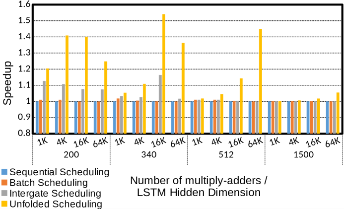
Figure 11 shows the performance comparison of the schedulers discussed in Section 5. Each set of 4 bars shows the speedups normalized to the first bar (Sequential scheduling). We evaluate the numbers considering all resource budgets and the LSTM models used for experimenting the design. Regarding the MVM tile-engine ($N\times$ $k$-width VS units), we consider 32 rows for the $k$ and mapping all the VS units to the columns of the weight matrix.

As Figure 11 depicts, Unfolded scheme always obtains the best performance of all, since it removes most of the data-dependencies and highly utilizes the parallel MACs. However, the benefit diminishes by increasing the LSTM dimension or reducing the number of MACs. The reason is that MVMs become the main performance bottleneck under those conditions, and hence, the way we order the LSTM computation cannot have the expected impact. On the other hand, Intergate scheduling outperforms Sequential and Batch scheduling. Comparing with our proposal, it provides less benefit as it only removes the intra-sequence dependency whereas across-sequence dependency still remains. Batch and Sequential schedules show almost similar execution, due to not efficiently handling all the data-dependencies.

Figure 11: Performance evaluation of the four schedulers for the different LSTM models and resource budgets. We consider sequence-length as 25 in all cases and similar size for hidden and input vectors. Speedup numbers are normalized to Sequential scheduling.

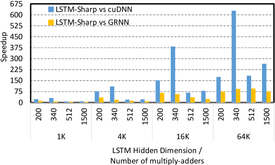
Figure 12 shows the execution time and resource-utilization considering the different resource budgets for SHARP and the LSTM models used for the design experimentation. The MVM tile-engine ($N\times$ $k$-width VS units) is configured based on the exploration result shown in Figure 9. Moreover, the tile is dynamically reconfigured to reduce the padding impact. As depicted, SHARP scales well as it linearly reduces the execution time (AVG case) by increasing the number of MACs from 1K to 64K. Furthermore, we obtain relatively high utilization for all the cases, ranging from 50% to 98% for 64K- to 1K-MAC resource-budgets, respectively. Compared to the ASIC-based EPUR architecture, resulting 24%, 49%, 74%, and 95% utilization for 1K-64K configurations, our design scales better for a variety of resource-budgets, particularly when increasing MAC units (1.3x - 2x). These performance benefits come form both the efficient scheduling as well as the reconfigurability of SHARPs’ architecture. With scheduling, we efficiently distribute the workload among different pipeline stages, whereas by reconfigurable MVM-tiling, we decide on the amount of work assigned for each stage. Consequently, by relaxing the two main dependencies of LSTM-computation, we are able to manage the resources more effectively.

Figure 12: Latency and resource-utilization of SHARP for different LSTM models and resource budgets. We consider sequence-length as 25 in all cases and similar size for hidden and input vectors.

We compare SHARP against the state-of-the-art GPU, FPGA and ASIC implementations, i.e. cuDNN [20], GRNN [23], BrainWave [24] and E-PUR [21]. We show the hardware specification of each of these platform in Table  3. Figure 13 shows the speedup achieved for the SHARP compared to the most recent scalable, efficient implementations on GPU. We use NVIDIA Titan V for the GPU evaluation that has a theoretical peak throughput of 29.8 TFLOPs (FP16). Speedup numbers are reported for all the different configuration, executing the various LSTM models that we have tested. As seen, our ASIC implementation outperforms the GPU’s in almost all the cases by up to 1 to 2 orders of magnitude. Considering 64K-MAC configuration, which has equal peak throughput as Titan V, SHARP obtains 172-625x and 72-93x faster LSTM inference than the cuDNN and GRNN GPU implementations.

Table 3: Hardware Configurations.

Architecture	#cores	Clock Speed(MHz)	Compute Precision	Power (W)
Titan V	5120	1200	float16	250
BrainWave	96000	250	float16	125
EPUR	1024	500	float16	1

Figure 13: SHARP’s speedup versus the most recent GPU implementations.

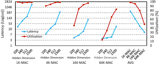
Table 4 shows the performance speedup achieved by our accelerator compared to the Stratix-10 version of BrainWave. Note that we reduce SHARP’s frequency from 500 MHz to 250 MHZ, similar to the BrainWave’s design, so as to have a fair comparison. In addition, we increase our MACs to 96K to have equal resource budget. We choose the LSTM configurations form Baidu DeepBench [38], similar to BrainWave’s experiments. As seen, we achieve more than 1.65x speedup for all the LSTM models and the speedups are significantly larger for the smaller dimensions. This shows that we alleviate the adaptability issue of BrainWave (see Figure 3).

Table 4: DeepBench LSTM Inference speedup over BrainWave [24].

LSTM hidden dimension	Time-steps	Speedup (X)
256	150	5.39
512	25	3.57
1024	25	1.85
1536	50	1.73

Furthermore, we compare LSTM performance considering several real-world application in Speech Recogniton, Video Captioning and also Machine Translation. Table 5 shows the configuration of the different networks used for measuring the performance evaluation. Table 6 shows the speedup SHARP achieves when running each network compared to E-PUR for the different number of MACs. Note that we use the same clock frequency of 500 MHz for both EPUR and SHARP. The results show that we obtain relatively higher speedups as we increase the number of resources. As a result, we improve the scalability of RNN acceleration for a range of resource budgets and different models.

Table 5: LSTM Network’s Configuration

Benchmark	Layers	LSTM	Hidden	Time
		Type	Units	Steps
EESEN [8]	5	Bi-dir	340	300-700
GMAT [39]	17	Uni-dir	1024	50-100
BYSDNE [40]	5	Uni-dir	340	30
RLDRADSPR [41]	10	Stacked	1024	300-512

Table 6: SHARP’s speedups w.r.t. EPUR [21]

Number of MACs	1K	4K	16K	64K
EESEN	1.07	1.25	1.68	1.9
GMAT	1.01	1.51	1.53	1.66
BYSDNE	1.05	1.24	1.8	2.22
RLDRADSPR	1.03	1.11	1.45	2.3

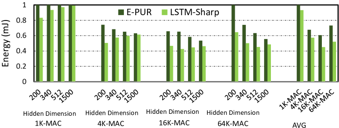
Furthermore, we measure the energy consumption for both SHARP and E-PUR considering different number of resources while using the same clock frequency. Figure 14 shows the energy consumption, normalized to E-PUR using 1K MACs, for the different LSTM dimensions. As it illustrates, SHARP obtains better energy-efficiency for the smaller models when there is lower resources available (1K- and 4K-MAC). This is due to the effectiveness of both Unfolded scheduling as well as flexible tiling. Moreover, reconfiguration handles the padding of LSTM’s MVM which is critical for the performance of smaller models and when there is less number of MACs (Figure 10). Moreover, we achieve higher energy-reduction for larger SHARP’s designs, as we achieve better scalability than E-PUR (Table 6) through efficiently utilizing SHARP’s MAC resources. Note that even though we increase power dissipation by between 1.4% to 36%, as the LSTM inference takes less time, therefore our energy numbers, which is $power\times time$, decreases more. In total, we reduce SHARP’s energy consumption on average by 7.3%, 18.2%, 34.8%, and 40.5% when using 1K to 64K MACs, respectively.

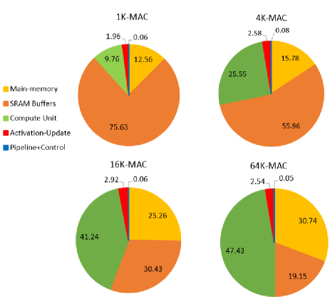
Figure 15 depicts the breakdown of power dissipation among the main components of our design. We consider an average case to compute the power for the different resource-budgets. As the figure illustrates, a large share of the power goes to the SRAM buffers, which is the dominant consumer for 1K- and 4K-MAC configurations. On the other hand, as we increase the number of resources, the compute-unit dissipates more power. Furthermore, main memory consumes more power and energy as the number of MACs grows, due to the high bandwidth requirement. The activation part takes almost similar amount of power as it does not change between different designs. Finally, the pipeline controller which also includes the reconfiguration logic has less than 1% share of the total power.

9 Related Work

Figure 14: Energy consumption of the SHARP for different hidden dimensions. The numbers are normalized to E-PUR with 1K-MAC resources.

Figure 15: Power breakdown of SHARP for different resource configurations. We average the percentages for running different applications. SHARP consumes 8.11, 11.36, 22.13, 47.7 Watts of power under 1K to 64K MACs.

To optimize the performance and energy of RNNs, a plethora of customized architecture [21, 29, 27] and neural-processing [28, 24] designs have been recently proposed in order . Most of the previous accelerators’ implementation are FPGA-based [42, 43, 24], whereas only a few works have been explored for ASIC design [28, 21]. Furthermore, these designs are either targeted for mobiles and wearables [21], or data centers and cloud networks [24, 28]. The latter cases normally restrict themselves to a relatively small resource budget, whereas the former employ a large amount of parallelism. SHARP aims to optimize RNN for a variety of design points and considering different model characteristics.

We have gone through some of the previous works [24, 28, 21] throughout the paper and compare them against SHARP’s evaluation results in Section 8. The rest implementations focus on two main problems for RNN acceleration: optimizing the inference computation [44, 45], and reducing memory requirements by compression and pruning techniques [29, 27].

In this paper, we mainly target dense and uncompressed RNN models. Furthermore, we consider that all the synaptic weights fit on-chip for one layer execution, similar to E-PUR [21] and BrainWave [24]. Other designs, such as ESE [8] and C-LSTM [27], take another approach that tries to pipeline the memory fetches with the LSTM computations in order to hide the latency of accessing off-chip data. However, we observe that such design schemes cannot provide good scalability and performance efficiency with high amount of parallelism, resulting in low utilization. We build SHARP in a way to optimize for various purposes from wearables to mobile systems and cloud networks. Also, we ensure that it achieves a scalable performance for a range of models.

Apart from FGPA and ASIC, researchers and practitioners are also looking into using GPUs for RNN [46, 47, 22]. They are mainly designed for maximizing training throughput, whereas the GPU utilization is limited by insufficient parallelism when the model size and batch size are small, which is difficult to make full usage of massive GPU cores.

10 Conclusions

In this paper, we propose SHARP, a scalable, high-performance RNN accelerator, which consists of a novel scheduling scheme — Unfolded that strictly overlaps the LSTM computation by hiding almost all the dependencies, and a dynamically reconfigurable architecture to improve the adaptability. SHARP tailors the resource allocation based on the requirements of a particular model. It achieves significant performance speedup, energy-saving and utilization improvement, for all the design points and various RNN models. Compared to the state-of-the-art ASIC, FPGA, and GPU implementations, we improve the performance by 2x, 2.8x, and 82x, respectively, considering 64K-MAC. Our scheme can also be applied for FPGAs, e.g. BrainWave, besides being targeted for ASIC design. Finally, we obtain an average utilization of 50%, for a peak throughput of 30 TFLOPs/s, resulting in 0.32 TFLOPS/Watt which is 1.7x and 7.4x more energy-efficient than current ASIC and FPGA implementations, respectively.

11 Acknowledgment

This work has been supported by the CoCoUnit ERC Advanced Grant of the EU’s Horizon 2020 program (grant No 833057), the Spanish State Research Agency (MCIN/AEI) under grant PID2020-113172RB-I00, and the ICREA Academia program.

References

- [1] Sepp Hochreiter and Jürgen Schmidhuber. Long short-term memory. Neural Computation, 9(8):1735–1780, 1997.
- [2] Junyoung Chung, Çaglar Gülçehre, KyungHyun Cho, and Yoshua Bengio. Empirical evaluation of gated recurrent neural networks on sequence modeling. CoRR, abs/1412.3555, 2014.
- [3] Hojjat Salehinejad, Julianne Baarbe, Sharan Sankar, Joseph Barfett, Errol Colak, and Shahrokh Valaee. Recent advances in recurrent neural networks. CoRR, abs/1801.01078, 2018.
- [4] Ilya Sutskever, Oriol Vinyals, and Quoc V. Le. Sequence to sequence learning with neural networks. CoRR, abs/1409.3215, 2014.
- [5] Oriol Vinyals, Alexander Toshev, Samy Bengio, and Dumitru Erhan. Show and tell: A neural image caption generator. CoRR, abs/1411.4555, 2014.
- [6] Jeff Donahue, Lisa Anne Hendricks, Sergio Guadarrama, Marcus Rohrbach, Subhashini Venugopalan, Kate Saenko, and Trevor Darrell. Long-term recurrent convolutional networks for visual recognition and description. CoRR, abs/1411.4389, 2014.
- [7] Subhashini Venugopalan, Marcus Rohrbach, Jeff Donahue, Raymond J. Mooney, Trevor Darrell, and Kate Saenko. Sequence to sequence - video to text. CoRR, abs/1505.00487, 2015.
- [8] Yajie Miao, Mohammad Gowayyed, and Florian Metze. EESEN: end-to-end speech recognition using deep RNN models and wfst-based decoding. CoRR, abs/1507.08240, 2015.
- [9] Kyunghyun Cho, Bart van Merrienboer, Çaglar Gülçehre, Fethi Bougares, Holger Schwenk, and Yoshua Bengio. Learning phrase representations using RNN encoder-decoder for statistical machine translation. CoRR, abs/1406.1078, 2014.
- [10] Min Joon Seo, Aniruddha Kembhavi, Ali Farhadi, and Hannaneh Hajishirzi. Bidirectional attention flow for machine comprehension. CoRR, abs/1611.01603, 2016.
- [11] Haichao Zhu, Li Dong, Furu Wei, Wenhui Wang, Bing Qin, and Ting Liu. Learning to ask unanswerable questions for machine reading comprehension. CoRR, abs/1906.06045, 2019.
- [12] Shuohang Wang and Jing Jiang. An lstm model for cloze-style machine comprehension. In Computational Linguistics and Intelligent Text Processing: 19th International Conference, 2018.
- [13] Tomas Mikolov, Martin Karafiát, Lukas Burget, Jan Cernocký, and Sanjeev Khudanpur. Recurrent neural network based language model, 01 2010.
- [14] Yair Lakretz, Germán Kruszewski, Theo Desbordes, Dieuwke Hupkes, Stanislas Dehaene, and Marco Baroni. The emergence of number and syntax units in LSTM language models. CoRR, abs/1903.07435, 2019.
- [15] Sarath Chandar, Chinnadhurai Sankar, Eugene Vorontsov, Samira Ebrahimi Kahou, and Yoshua Bengio. Towards non-saturating recurrent units for modelling long-term dependencies. CoRR, abs/1902.06704, 2019.
- [16] Daniel S. Park, William Chan, Yu Zhang, Chung-Cheng Chiu, Barret Zoph, Ekin D. Cubuk, and Quoc V. Le. Specaugment: A simple data augmentation method for automatic speech recognition. Interspeech 2019, Sep 2019.
- [17] M. W. Y. Lam, X. Chen, S. Hu, J. Yu, X. Liu, and H. Meng. Gaussian process lstm recurrent neural network language models for speech recognition. In ICASSP 2019, pages 7235–7239, May 2019.
- [18] Wojciech Zaremba, Ilya Sutskever, and Oriol Vinyals. Recurrent neural network regularization. CoRR, abs/1409.2329, 2014.
- [19] Yonghui Wu, Mike Schuster, Zhifeng Chen, Quoc V. Le, Mohammad Norouzi, Wolfgang Macherey, Maxim Krikun, Yuan Cao, Qin Gao, Klaus Macherey, Jeff Klingner, Apurva Shah, Melvin Johnson, Xiaobing Liu, Lukasz Kaiser, Stephan Gouws, Yoshikiyo Kato, Taku Kudo, Hideto Kazawa, Keith Stevens, George Kurian, Nishant Patil, Wei Wang, Cliff Young, Jason Smith, Jason Riesa, Alex Rudnick, Oriol Vinyals, Greg Corrado, Macduff Hughes, and Jeffrey Dean. Google’s neural machine translation system: Bridging the gap between human and machine translation. CoRR, abs/1609.08144, 2016.
- [20] Sharan Chetlur, Cliff Woolley, Philippe Vandermersch, Jonathan Cohen, John Tran, Bryan Catanzaro, and Evan Shelhamer. cudnn: Efficient primitives for deep learning. CoRR, abs/1410.0759, 2014.
- [21] Franyell Silfa, Gem Dot, Jose-Maria Arnau, and Antonio Gonzàlez. E-pur: An energy-efficient processing unit for recurrent neural networks. PACT ’18, pages 18:1–18:12, New York, NY, USA, 2018. ACM.
- [22] Jeremy Appleyard, Tomás Kociský, and Phil Blunsom. Optimizing performance of recurrent neural networks on gpus. CoRR, abs/1604.01946, 2016.
- [23] Connor Holmes, Daniel Mawhirter, Yuxiong He, Feng Yan, and Bo Wu. Grnn: Low-latency and scalable rnn inference on gpus. In EuroSys ’19, pages 41:1–41:16, Dresden, Germany, 2019.
- [24] J. Fowers, K. Ovtcharov, M. Papamichael, T. Massengill, M. Liu, D. Lo, S. Alkalay, M. Haselman, L. Adams, M. Ghandi, S. Heil, P. Patel, A. Sapek, G. Weisz, L. Woods, S. Lanka, S. K. Reinhardt, A. M. Caulfield, E. S. Chung, and D. Burger. A configurable cloud-scale dnn processor for real-time ai. In ISCA’45, pages 1–14, June 2018.
- [25] Scott Yokim. Tensor ops made easier in cudnn. https://devblogs.nvidia.com/tensor-ops-made-easier-in-cudnn/, 2018.
- [26] Minjia Zhang, Samyam Rajbhandari, Wenhan Wang, and Yuxiong He. Deepcpu: Serving rnn-based deep learning models 10x faster. In 2018 USENIX Annual Technical Conference, pages 951–965, Boston, MA, 2018.
- [27] Shuo Wang, Zhe Li, Caiwen Ding, Bo Yuan, Yanzhi Wang, Qinru Qiu, and Yun Liang. C-LSTM: enabling efficient LSTM using structured compression techniques on fpgas. CoRR, abs/1803.06305, 2018.
- [28] Norman P. Jouppi, Cliff Young, Nishant Patil, David Patterson, Gaurav Agrawal, Raminder Bajwa, Sarah Bates, Suresh Bhatia, Nan Boden, Al Borchers, Rick Boyle, Pierre-luc Cantin, Clifford Chao, Chris Clark, Jeremy Coriell, Mike Daley, Matt Dau, Jeffrey Dean, Ben Gelb, Tara Vazir Ghaemmaghami, Rajendra Gottipati, William Gulland, Robert Hagmann, C. Richard Ho, Doug Hogberg, John Hu, Robert Hundt, Dan Hurt, Julian Ibarz, Aaron Jaffey, Alek Jaworski, Alexander Kaplan, Harshit Khaitan, Daniel Killebrew, Andy Koch, Naveen Kumar, Steve Lacy, James Laudon, James Law, Diemthu Le, Chris Leary, Zhuyuan Liu, Kyle Lucke, Alan Lundin, Gordon MacKean, Adriana Maggiore, Maire Mahony, Kieran Miller, Rahul Nagarajan, Ravi Narayanaswami, Ray Ni, Kathy Nix, Thomas Norrie, Mark Omernick, Narayana Penukonda, Andy Phelps, Jonathan Ross, Matt Ross, Amir Salek, Emad Samadiani, Chris Severn, Gregory Sizikov, Matthew Snelham, Jed Souter, Dan Steinberg, Andy Swing, Mercedes Tan, Gregory Thorson, Bo Tian, Horia Toma, Erick Tuttle, Vijay Vasudevan, Richard Walter, Walter Wang, Eric Wilcox, and Doe Hyun Yoon. In-datacenter performance analysis of a tensor processing unit. In Proceedings of the 44th Annual International Symposium on Computer Architecture, ISCA ’17, pages 1–12, New York, NY, USA, 2017. ACM.
- [29] Song Han, Junlong Kang, Huizi Mao, Yiming Hu, Xin Li, Yubin Li, Dongliang Xie, Hong Luo, Song Yao, Yu Wang, Huazhong Yang, and William J. Dally. ESE: efficient speech recognition engine with compressed LSTM on FPGA. CoRR, abs/1612.00694, 2016.
- [30] Synopsys. Synopsys. https://www.synopsys.com/, 2010.
- [31] Synopsys. Synopsys designware library. https://www.synopsys.com/dw/buildingblock.php, 2021.
- [32] S. Li, K. Chen, J. H. Ahn, J. B. Brockman, and N. P. Jouppi. Cacti-p: Architecture-level modeling for sram-based structures with advanced leakage reduction techniques. In IEEE/ACM ICCAD, 2011.
- [33] TN-41-01. Calculating memory system power for ddr3, micron technology, tech. rep. Technical report, 2007.
- [34] J. A. Hartigan and M. A. Wong. Algorithm as 136: A k-means clustering algorithm. Journal of the Royal Statistical Society. Series C (Applied Statistics), 28(1):100–108, 1979.
- [35] Hamid Tabani, Jose-Maria Arnau, Jordi Tubella, and Antonio González. An ultra low-power hardware accelerator for acoustic scoring in speech recognition. In 2017 26th International Conference on Parallel Architectures and Compilation Techniques (PACT), pages 41–52, 2017.
- [36] Song Han, Huizi Mao, and William J. Dally. Deep compression: Compressing deep neural networks with pruning, trained quantization and huffman coding, 2016.
- [37] Udit Gupta, Brandon Reagen, Lillian Pentecost, Marco Donato, Thierry Tambe, Alexander M. Rush, Gu-Yeon Wei, and David Brooks. Masr: A modular accelerator for sparse rnns. In 2019 28th International Conference on Parallel Architectures and Compilation Techniques (PACT), pages 1–14, 2019.
- [38] S. Narang and G. Diamo. Baidu deepbench. https://github.com/baidu-research/DeepBench, 2017.
- [39] Yonghui Wu, Mike Schuster, Zhifeng Chen, Quoc V. Le, Mohammad Norouzi, Wolfgang Macherey, Maxim Krikun, Yuan Cao, Qin Gao, Klaus Macherey, Jeff Klingner, Apurva Shah, Melvin Johnson, Xiaobing Liu, Łukasz Kaiser, Stephan Gouws, Yoshikiyo Kato, Taku Kudo, Hideto Kazawa, Keith Stevens, George Kurian, Nishant Patil, Wei Wang, Cliff Young, Jason Smith, Jason Riesa, Alex Rudnick, Oriol Vinyals, Greg Corrado, Macduff Hughes, and Jeffrey Dean. Google’s neural machine translation system: Bridging the gap between human and machine translation, 2016.
- [40] Joe Yue-Hei Ng, Matthew Hausknecht, Sudheendra Vijayanarasimhan, Oriol Vinyals, Rajat Monga, and George Toderici. Beyond short snippets: Deep networks for video classification, 2015.
- [41] Jaeyoung Kim, Mostafa El-Khamy, and Jungwon Lee. Residual lstm: Design of a deep recurrent architecture for distant speech recognition, 2017.
- [42] Andre Xian Ming Chang, Berin Martini, and Eugenio Culurciello. Recurrent neural networks hardware implementation on FPGA. CoRR, abs/1511.05552, 2015.
- [43] Javier Hoffmann, Osvaldo Navarro Guzmán, Florian Kästner, Benedikt Janßen, and Michael Hübner. A survey on cnn and rnn implementations. In The Seventh International Conference on Performance, Safety and Robustness in Complex Systems and Applications, pages 33–39, Venice, Italy, 2017. CYBER.
- [44] Y. Guan, Z. Yuan, G. Sun, and J. Cong. Fpga-based accelerator for long short-term memory recurrent neural networks. In 22nd ASP-DAC, pages 629–634, Jan 2017.
- [45] S. Li, C. Wu, H. Li, B. Li, Y. Wang, and Q. Qiu. Fpga acceleration of recurrent neural network based language model. In 2015 IEEE 23rd Annual International Symposium on Field-Programmable Custom Computing Machines, pages 111–118, May 2015.
- [46] Greg Diamos, Shubho Sengupta, Bryan Catanzaro, Mike Chrzanowski, Adam Coates, Erich Elsen, Jesse Engel, Awni Y. Hannun, and Sanjeev Satheesh. Persistent RNNs: Stashing Recurrent Weights On-Chip. In Proceedings of the 33nd International Conference on Machine Learning, ICML ’16, pages 2024–2033, 2016.
- [47] Felix Weninger, Johannes Bergmann, and Björn Schuller. Introducing CURRENNT: The Munich Open-source CUDA Recurrent Neural Network Toolkit. Journal of Machine Learning Research, 16(1):547–551, 2015.