Dynamical adaptivity for LES of compressible flows in a high order DG framework
Abstract
We investigate the possibility of reducing the computational burden of LES models by employing locally and dynamically adaptive polynomial degrees in the framework of a high order DG method. A degree adaptation technique especially featured to be effective for LES applications, that was previously developed by the authors and tested in the statically adaptive case, is applied here in a dynamically adaptive fashion. Two significant benchmarks are considered, comparing the results of adaptive and non adaptive simulations. The proposed dynamically adaptive approach allows for a significant reduction of the computational cost of representative LES computation, while allowing to maintain the level of accuracy guaranteed by LES carried out with constant, maximum polynomial degree values.
(1) Dipartimento di Scienze e Tecnologie Aerospaziali, Politecnico di Milano
Via La Masa 34, 20156 Milano, Italy
antonella.abba@polimi.it, alessandro.recanati@mail.polimi.it, matteo.tugnoli@polimi.it
(2) MOX – Modelling and Scientific Computing,
Dipartimento di Matematica, Politecnico di Milano
Piazza Leonardo da Vinci, 20133 Milano, Italy
luca.bonaventura@polimi.it
Keywords: Turbulence modelling, Large Eddy Simulation, Discontinuous Galerkin methods, compressible flows, dynamic models.
AMS Subject Classification: 65M60, 65Z05, 76F25, 76F50, 76F65
1 Introduction
During the last decades, Large Eddy Simulation (LES) has been extensively studied and has allowed to achieve results comparable to those of Direct Numerical Simulations (DNS) with a significant reduction in computational cost, enabling the use of high accuracy models to simulate turbulent flows beyond the extremely idealized configurations to which DNS was typically limited. While the increase of the available computing power makes even more fluid flow configurations amenable to LES approaches, two interlinked difficulties prevent LES from being a widespread tool for industrial applications. The first major issue is that LES simulations, due to their space and time resolution requirements, are still very computationally expensive. The second is that selecting the right spatial resolution for an LES of a unsteady turbulent flow in a complex geometry is not a easy task. On one hand, the resolution must be sufficient to solve the equations with adequate accuracy, but limited to contain the computational costs. On the other hand, the implicit LES (ILES) commonly employed uses the discretization as the filter, so that the mesh resolution sets implicitly the filter width and the threshold between the resolved scales and the modelled ones. Moreover, in a turbulent flow in complex geometry, turbulence characteristics change in time and in space throughout the computational domain and cannot be as easily estimated as it was the case in the simple geometries employed for many years in LES studies. Therefore, an adaptive LES, where the resolution and the filter width are automatically adapted to the flow conditions, would be of great benefit for the solution of both problems, in order to have an LES with the correct filter sizing and an efficient spatial discretization. The problem of estimating the right resolution is further complicated by the fact that, as pointed out by the authors in [34], using standard error estimators to adapt the resolution is not the optimal approach for LES, if refinement to DNS resolutions is to be avoided, so that specific strategies must be devised in this context.
The need of an adaptive LES was first stated by [26], but not many attempts have been made in this direction since then. In the numerical solution of PDEs, however, in the last decades considerable efforts have been devoted to the development of refinement indicators. Most of these are based on local estimates of the discretization error, see e.g. [4, 5, 20, 28, 29, 37, 36, 35, 39]. In the LES context, however, simply increasing the resolution in order to decrease the error leads to a DNS solution [23, 29], which is in contrast with the goal of adaptive LES, which consists in adjusting the resolution in order to directly resolve only a prescribed amount of the turbulent scales. An alternative approach, pursued e.g. in [17, 19, 18], employs indicators aimed at obtaining a good representation of some quantity of interest, rather than of the physical scales of the turbulence. Adjoint–based adaptation methods proposed by other authors [11] have also shown good performance, but entail significant computational costs.
In the present work, we will consider a physically based refinement indicator proposed by the authors in [34, 31], which is especially suited for LES. This adaptivity approach is implemented in a numerical framework based on the Discontinuous Galerkin (DG) method, that was already presented and validated in [1], which allows to extend seamlessly LES concept to unstructured meshes. DG methods combine the high order of accuracy and low dissipation/dispersion properties with good parallel performances, since most of the computations are local to the element and only inter-element boundary fluxes must be communicated. The adaptation technique we employ is a adaptive approach, in which the polynomial degree is varied locally, rather than the mesh size, as in more standard adaptive methods. DG methods provide an interesting environment for adaptivity, since they do not require to enforce continuity constraints at the interelement boundaries. Furthermore, adaptive techniques are appealing since they allow to correct possible shortcomings of the computational mesh, as well as to perform dynamically adaptive simulations without extensive remeshing. Static polynomial adaptivity was applied to LES in [10, 34, 24, 31] to efficiently simulate statistically steady phenomena, while an example of dynamical adaptation is described in [11] in an ILES context.
In this paper, we will show how the adaptive method of [34, 31] can be applied locally and dynamically in time, in order to simulate efficiently and accurately transient phenomena. A number of time dependent numerical simulations of two different configurations is considered, namely a temporally evolving mixing layer and the interaction of a vortex impinging on a square cylinder with the cylinder wake. The results obtained show that a significant reduction of the computational cost of LES can be achieved, reducing the number of degrees of freedom employed to values of up to of those required by constant maximum polynomial degree simulations, while maintaining essentially the same level of accuracy.
In Section 2, the model equations and numerical method are reviewed. In Section 3, the dynamical adaptivity approach we propose is outlined. In Sections 4, 5, results of numerical simulations on two significant benchmarks are presented. Finally, in Section 6 some conclusions are drawn and some perspectives of future development of this approach are discussed.
2 Model equations and numerical method
In this Section, the model equations and the numerical method will be briefly illustrated. For a more detailed description, we refer to [1], where this methodology was first introduced and validated for LES applications. The LES filtered Navier–Stokes equations for compressible flows can be written in dimensionless form as:
| (1) |
where are the prognostic resolved variables and are the fluxes, composed by the advective fluxes
| (2) |
the viscous fluxes
| (3) |
and finally the subgrid fluxes
| (4) |
Here, and represent the grid filter and the Favre filter operators, so that denotes the filtered pressure, the resolved enthalpy and and the momentum and heat diffusive fluxes, respectively. Equations (1) are completed by the dimensionless state equation for a perfect gas
| (5) |
where is the filtered temperature. To close the system the constitutive equations must also be specified:
| (6) |
where the rate of resolved strain tensor is defined as
| (7) |
and the dynamic viscosity, according to a power law, is
| (8) |
with . In the Local Discontinuous Galerkin approach [8], the equations are rewritten as a first order system
| (9) | |||||
| (10) |
where . A tessellation composed of non overlapping tetrahedral elements is defined in the domain over which a discontinuous finite element space is defined in the following way
| (11) |
where denotes the space of polynomial functions of total degree . The weak discrete form of equation (9) is derived using test functions belonging to the same space as the numerical solution. A modal DG approach is here applied, by using a hierarchical orthonormal polynomial basis for each element in the finite dimensional space to represent the numerical approximation of the generic variable expressed as
| (12) |
where are the basis functions on element are the modal coefficients of the basis functions and is the number of basis functions required to span the polynomial space of degree , defined in as:
| (13) |
To compute the advective flux the Rusanov flux [21] is employed while a centred flux is used for the diffusive fluxes , and for the gradient variables flux .
In the present framework, as explained in detail in [1], the filtering operators are built in the DG spatial discretization, so that the LES filtering is equivalent to the projection onto the employed finite dimensional solution subspace
| (14) |
while Favre filter operator is defined as
| (15) |
In the simulations presented in this paper, two different subgrid models have been employed, the classical Smagorinsky model, in which the filter width is determined as
| (16) |
and the anisotropic dynamic model [1, 3], in which the filter width is included in the coefficients to be dynamically determined [2] using the Germano identity [15].
3 A dynamically adaptive approach
A physically based refinement indicator especially suited for LES has been proposed by the authors in [34, 31]. This indicator is based on the classical structure function
| (17) |
where represents the expected value operator. The structure function has been widely used to study turbulence statistics and it is known to be directly related to subgrid stresses [6, 7, 14]. Larger values of the structure function calculated inside the element denote a poorly correlated velocity field, and the need of a higher resolution, while lower values denote a highly correlated velocity field, which is an indication of a very well resolved turbulent region or laminar conditions, hence the possibility of employing a lower resolution. The degree adaptation indicator is then defined as:
| (18) |
where is the structure function in isotropic conditions [25].
In [34], this procedure was shown to be effective in a statically adaptive framework, producing accurate results with a significant reduction in the computational cost. However, static adaptivity presents some limitations, since the resolution is fixed at the beginning of the simulation and constant in time. In the simulation of a transient phenomenon, for which a time resolved solution is sought rather than a statistical average, employing a dynamic adaptivity framework is necessary. In our implementation of the dynamic degree adaptation, indicator (18) is computed at runtime at time intervals and averaged over time. Once the indicator has been averaged on a time interval which is sufficiently larger than but still small with respect to the time scale of the motion of the main turbulent structures, a new polynomial distribution is computed based on the indicator values and the flow field approximation is updated, by either reducing or increasing the number of degrees of freedom employed in each element.
In this work, the admissible polynomial degrees ranged from 2 to 4. Two indicator thresholds were employed. Cells with a value of the indicator (18) lower than the smaller threshold were assigned the lowest allowed polynomial degree 2, those with value higher than the largest threshold were assigned the highest polynomial degree 4 and the intermediate ones were assigned degree 3. Polynomial degrees were only allowed to be increased or decreased by one degree at each adaptation time. Since the solution is represented by a hierarchical basis, when lowering the polynomial degree, the contribution associated to the removed modes is simply discarded, while when raising the polynomial degree the coefficients of the newly added modes are initialized to zero, to be updated by the subsequent time evolution.
It should be remarked that the procedure outlined above can potentially lead to unbalances between the computational load of different processors in a parallel run. The implementation of a full dynamic load balancing is beyond the scope of the present work, whose focus is mostly on the assessment of the accuracy of the above methodology. As a consequence, in all the numerical experiments presented below, the computational load among the processors is approximately balanced at the beginning of the simulation only, which is clearly suboptimal with respect to full parallel efficiency. Indeed, the results will not in general be assessed based of the CPU time required, but rather on the total number of the degrees of freedom employed in the adaptive versus non adaptive simulations. However, it must be noted that,t even with this suboptimal configuration, the adaptive simulation always led to a net reduction in computational effort. In order to assess the effective reduction in the CPU time required, further work on code optimization is needed, along with the development and application of load balancing approaches such as those employed e.g. in [11, 40].
4 Temporally evolving mixing layer
In a first assessment of the adaptive LES approach outlined in the previous sections, an isothermal time developing mixing layer was simulated. The temporal mixing layer represents an interesting test case for LES, due to its simplicity and advantages from the computational viewpoint, as well as the complexity of the physics related to the mixing, see e.g. the discussions in [13, 30, 38, 41]. The commonly employed configuration to represent a mixing layer flow was employed, imposing periodic boundary conditions on the mean flow and in the span wise directions. Thanks to the periodicity in the stream wise direction, uncertainties related to the imposition of inlet and outlet boundary conditions are avoided. In the simulations presented here, the anisotropic dynamic subgrid model [1, 3] has been used, in which the filter width is included in the coefficients to be dynamically determined. A further application of this approach is presented in [2].
A sketch of the flow configuration is shown in Figure 1. The mixing layer is characterized by two parallel flows with different velocities and The convection velocity of the isothermal mixing layer, defined as , is the velocity that transports the cortical structures at the centreline. In the configuration we considered, the convection velocity is assumed to be zero, so that the eddies do not travel inside the domain by means of the flow, but only move by mutual interaction. As a consequence, and . The reference frame is chosen so that the axis is aligned with the main direction of the flow centred at the middle of the domain, while the and axis denote transverse and lateral directions, respectively. The initial vorticity thickness, defined as
is chosen as reference length for the non-dimensionalization. The initial velocity jump is used as reference velocity, the initial uniform density and temperature are used as reference density and temperature, respectively. The fundamental dimensionless groups are then
The temporally evolving mixing layer develops from a specified initial condition. In these computations, we use a hyperbolic tangent as the base velocity profile for the longitudinal component
| (19) |
where and so that . Similarly to [16, 12], a 3D incompressible disturbance is added to the base velocity profile to initiate the transition process. It consists of harmonic disturbances expressed as
where and the decay in -direction is governed by . Moreover, a 3D white noise perturbation is added to the initial velocity field, generated for each mesh node by a logistic map rescaled to take values on and multiplied by the attenuation factor Uniform pressure and density are used to initialize the simulation.
The longitudinal dimension of the computational domain must be large enough to allow at least for the merging of two principal vortical structure, so it must be taken as a multiple of the wavelength characterizing the most unstable perturbation, which according to the analysis in [30] is given in this context by In the present simulation, the size in the streamwise direction has been chosen so that up to three vortices are allowed to merge. In the normal direction, the computational domain extends for while in spanwise direction . Periodic boundary conditions are applied in the statistically homogeneous and directions, while a sponge layer is employed at the top and bottom boundaries, so that the effective size of the computational domain in the direction is equal to .
The computational mesh is built first subdividing the domain in hexahedra. Each hexahedron is then split into tetrahedra, yielding a total of tetrahedral elements. The actual resolution depends on the local polynomial order and can be computed as
For we get .
A preliminary study of the mixing layer in the present configuration was presented in [27], where the sensitivity of the results to the choice of spatial resolution and subgrid scale model was checked. The objective of the present work is to test the adaptivity technique in a time evolving flow. For this purpose, the results obtained with polynomial degree dynamically adapting in space and time are compared with the results obtained with constant fourth and third degree polynomials.
To set the values of the adaptation thresholds the structure function indicator was evaluated on the velocity field obtained with constant at the final dimensionless time Thresholds were then chosen in order to obtain, for that field, an adapted number of degrees of freedom (dofs) lower than of the corresponding number of dofs in the constant case. The resulting threshold values are then and . The dynamical adaptation was carried out by computing the indicator value at intervals and averaging them over intervals while the value was used for time integration.
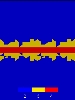
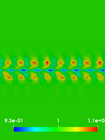
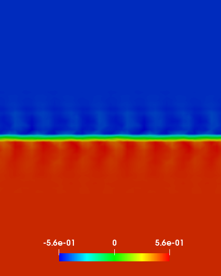
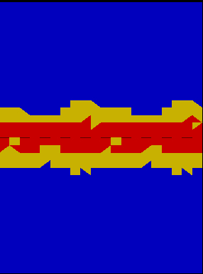
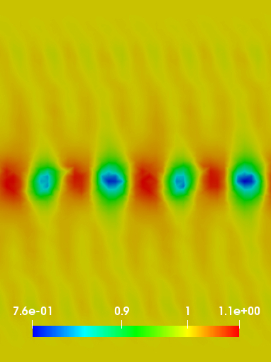
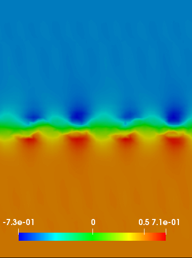

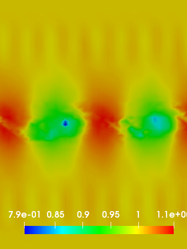
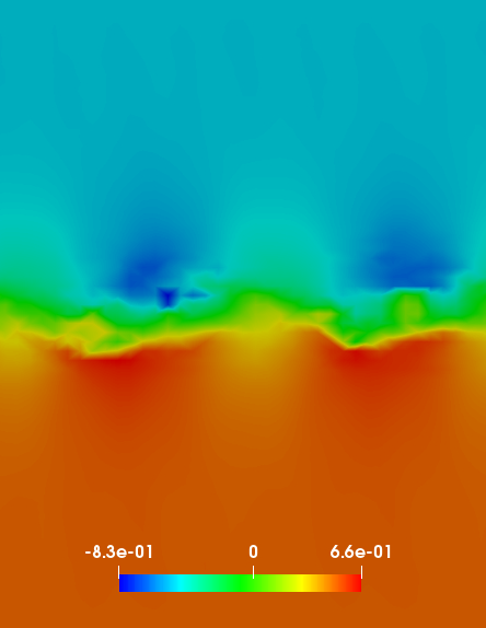
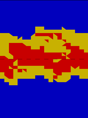
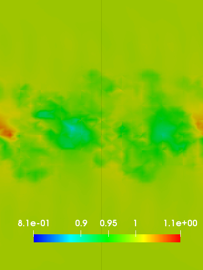
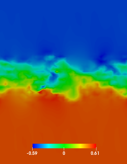
The polynomial degree distribution, the density and the streamwise component of the velocity, at different instants, in the plane , are represented in Figure 2. In the initial condition, the elements with highest degree are concentrated along the middle of the domain, where high resolution is required. Then, the region with higher polynomial degree extends in space during time, adapting to the merging of the vortices, to the diffusion of turbulent structures and to the growth of the layer thickness. An important quantity for the characterization of the mixing layer is the momentum thickness, defined as
| (20) |
The time evolution of this quantity is represented in Figure 3. Notice that slope variations in the time evolution are associated to the merging of the vortices. A difference in the behaviour of the simulation with respect to the one is evident after the second merging, while the adaptive simulations well reproduces the results.
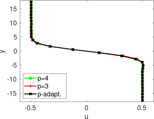
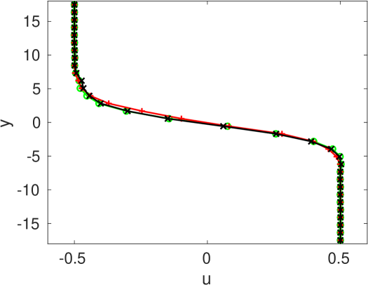
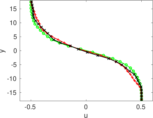
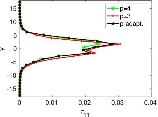
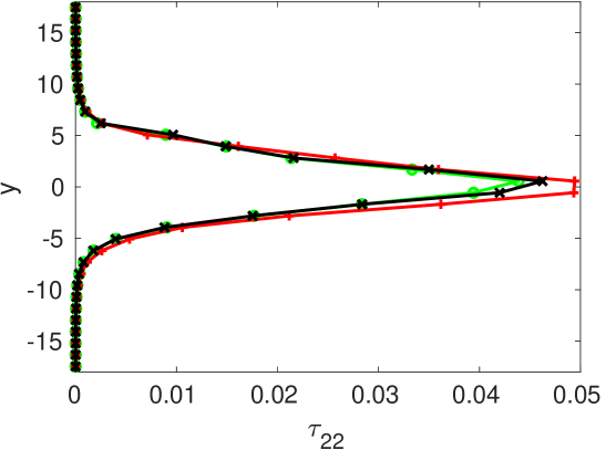
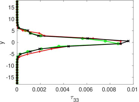
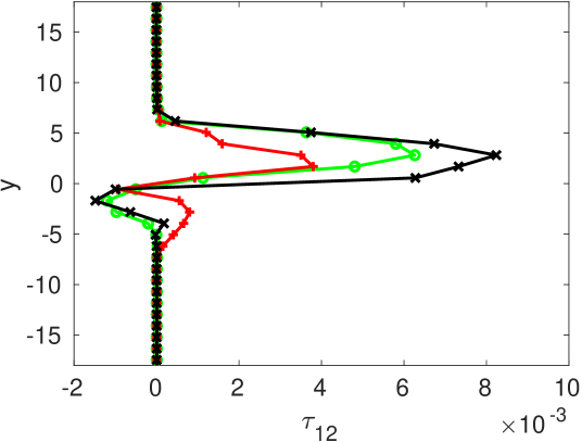
No relevant differences between the results obtained using adaptive or constant polynomial degree distribution are observed in the mean density and velocity profiles, shown in Figure 4, nor in the mean normal stresses profiles, shown in Figures 5(a)–5(c). Instead, looking at the shear stresses in Figure 5(d), although the peak is slightly overestimated, the adaptive solution is in good agreement with that of the case. From the same picture, the more dissipative character of the solution is also apparent.
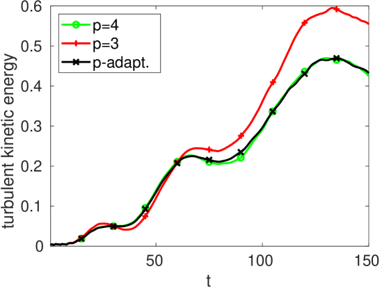
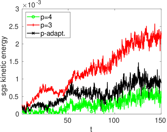
Looking at the turbulent kinetic energy profile in Figure 6, we can affirm that the turbulent energy amount of the flow is reproduced by the adaptive simulation with the same accuracy as in the case. In Figure 6, the subgrid scale (SGS) kinetic energy in the case is clearly larger than in the other cases, due to the lower resolution that requires more intense contribution from the model. The SGS energy for the adaptive case is closer to that of the case, demonstrating that the two simulations have an equivalent effective resolution.
All the simulations were carried out on the Marconi cluster at CINECA, using 272 KNL processors. In Figure 7, the total number of dofs for the adaptive simulation is shown as a function of time and compared with the values corresponding to uniform polynomial distributions, that are about and for and respectively. The gain using adaptivity is evident, since it requires less than of the dofs for and less then half of the dofs for the case. The core hours necessary to perform the simulations are reported in Table 1. In spite of the absence of a specific dynamic load balancing procedure, the adaptive technique also yields a reduction of the required CPU time, which has a value only marginally larger than that of the simulation. On the other hand, the sub-optimal nature of the present implementation is highlighted by the fact that the adaptive simulation required more CPU time than the case, even though it involved less dofs.
| Core hours | |
|---|---|
| 12600 | |
| 9000 | |
| adaptive | 9300 |
Concluding this analysis, we can affirm that the adaptive solutions display almost the same accuracy as those obtained with constant degree four, but require less then the half the number of dofs and about less CPU time for this test case, in spite of a sub-optimal implementation. Moreover, the structure function indicator which was proven successful in static adaptation in [34] is shown to be suitable also for simulation of transitional flows using a dynamic adaptation in time.
5 Interaction of Vortex and Square Section Cylinder
A body-vortex interaction flow represents another interesting time dependent problem to test dynamic adaptivity. Here, a vortex interacting with a square section cylinder at and is considered. This configuration was chosen because the analogous case without a vortex has already been studied with statically adaptive techniques in [34]. The classical Smagorinsky SGS model was applied for this test. The results obtained with polynomial adaptivity are compared with the solution obtained with uniform in space and constant in time degree distribution. The constant degree four solution is taken as reference.
The computational domain employed is box shaped and a 2D sketch of the geometry is represented in Figure 8. Denoting the cylinder side with , which is used as reference length, the inflow length has been taken equal to while the outflow length is equal to . The cylinder is vertically centred with a distance of from the upper and lower boundaries. The domain is extruded in the spanwise direction by a length equal to . This configuration was employed e.g. in [9] and has been used to assess statically adaptive LES simulations of the standard flow around a square section cylinder in [34, 31, 32].

Non-slip isothermal conditions are imposed on the cylinder walls, while Neumann conditions are imposed on the upper and lower boundaries of the domain and periodic conditions are enforced in the spanwise direction to simulate an infinite span cylinder. Dirichlet conditions with the far field values are imposed on the inflow and outflow, with sponge layers to avoid reflections of disturbances from the boundaries. At the inflow, a uniform far-field velocity is imposed.
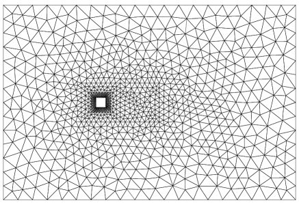
The mesh employed consists of 23816 tetrahedra arranged in an outer unstructured area and a structured O-grid mesh around the cylinder, which is then extruded in the spanwise direction. Considering a polynomial basis of degree 4, the resolution in space around the cylinder is in the wall normal direction, along the cylinder sides and along the spanwise direction. As in [34], the thresholds for the structure function (SF) indicator are taken to be so as to obtain a number of dofs just lower than the one obtained with uniform degree 3.
To simulate the cylinder-vortex interaction, a vortex is superimposed to an initial condition corresponding to a developed flow around the cylinder, obtained by a previous LES simulation. The introduced vortex is parallel to the direction and defined by the velocity components
| (21) | |||||
| (22) | |||||
| (23) |
where denotes the vortex strength, is the vortex radius, is the distance in the plane from the vortex centre and is the uniform flow over which the vortex is superimposed [22]. The maximum radial velocity is obtained at and is given by . Regarding the other variables, it is known from [9] that for a viscous compressible vortex the radial pressure distribution given by the solution of
| (24) |
Assuming a constant temperature distribution one obtains from (24) the profile
| (25) |
Finally the density distribution follows the equation of state
In [31, 33] simple advection of this vortex was tested. The maximum radial velocity chosen is and the vortex radius is . A reference simulation without vortex was used to calibrate the introduction time in order for the vortex to reach the cylinder in the instant of maximum lift. The dynamical adaptation strategy consisted in this case of adapting the polynomial degrees approximately three times during the time needed by a fluid particle to pass through the smallest elements on the cylinder walls at the free stream velocity . This choice led to computing the indicator value at intervals and averaging them over intervals while the value was used for time integration.
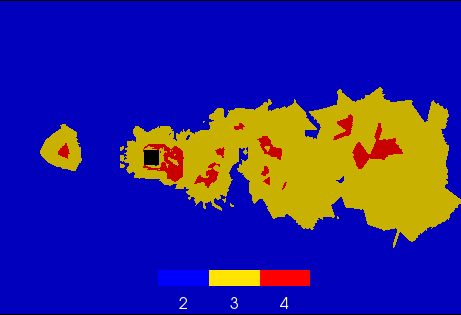
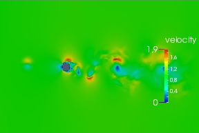
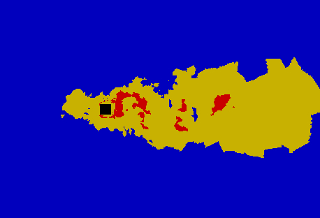
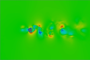
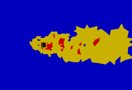
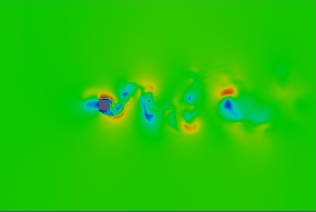
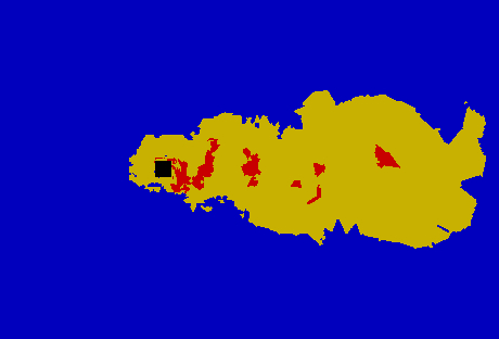
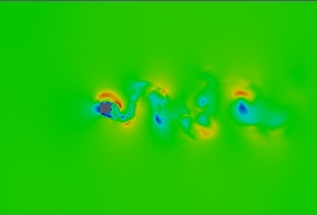
The dynamically adaptive procedure was able also in this case to effectively represent the structures of the flow, both in the advected vortex region and in the wake of the obstacle, as can be seen in Figures 10-13. It is possible to note that a higher polynomial degree is employed in the advected vortex region and in the shear layers around the cylinder. The dynamic adaptation procedure is able to effectively increase the polynomial degree around the vortex and to follow it as it is advected downstream, leaving all the elements with no vortex activity at the lowest resolution. Notice that the centre of the vortex is represented with degree 4 polynomials in the first instants, but only degree 3 polynomials are employed later, since the vortex enters an area with a more refined mesh in which a lower polynomial degree is sufficient.
(a)
 (b)
(b)
(a)
 (b)
(b)
(a)
 (b)
(b)
(a)
 (b)
(b)
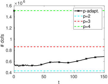
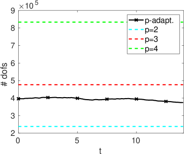
Among the different effects caused by the vortex-cylinder interaction, the most interesting are those on the forces acting on the cylinder. The history of the load coefficients before, during and after the interaction is reported in Figure 14.
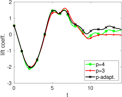
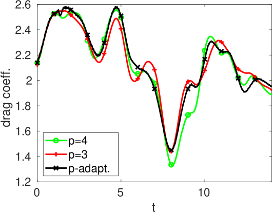
In the developed flow around the square cylinder, the periodic oscillation of the force coefficients are related to the unsteadiness of the recirculation bubble on the upper and lower sides and to the vortex shedding. Reaching the upper corner of the cylinder at , the vortex changes the pressure distribution on the front of the cylinder and strongly modifies the recirculating bubble on the upper side. In this condition, it is very important to use an adequate resolution on the upper side and in the separation bubble. In Figure 14 it can be observed that the peaks of the lift and drag coefficients at with adaptivity equal those in the reference solution demonstrating the capability of the proposed dynamically adaptive approach to well represent this unsteady phenomenon. The values of the differences of the peaks for the lift and drag coefficients with respect to the vortex free solution are reported in Table 2. Also in this case the values obtained with adaptivity are in very good agreement with the reference solution.
| configuration | peak diff. % | max diff. % | min diff. % |
|---|---|---|---|
| -24 | -0.01 | -39 | |
| -32 | -4 | -38 | |
| -24 | -0.01 | -38 |
The simulations were carried out on the Marconi cluster at CINECA, using 272 Brodwell processors. The adaptive simulation allows a reduction of about of the required CPU time with respect to the constant degree case. In Figure 15, the time history of the dofs number is shown. It is worth noting that, even though the number of dofs is affected by the flow regime inside the domain, its variations are anyway fairly limited and the total number remains less than the one employed for the uniform simulation. The core hours necessary to perform the simulations are reported in Table 3. Also in this case,the adaptive technique yields a reduction of the required CPU time, which has a value only marginally larger than that of the simulation. Again, the sub-optimal nature of the present implementation is highlighted by the fact that the adaptive simulation required more CPU time than the case, even though it involved less dofs.
| Core hours | |
|---|---|
| 756 | |
| 388 | |
| adaptive | 462 |
6 Conclusion
The need for adaptive LES approaches was first stated in [26], but adaptive LES simulations are not very common yet. DG methods provide a appropriate environment for adaptive approaches, since they do not require to enforce continuity constraints at the inter-element boundaries. Furthermore, adaptive techniques are appealing, since they allow to correct possible shortcomings of the computational mesh as well as to perform dynamically adaptive simulations without extensive remeshing.
Static polynomial adaptivity has been applied to LES in a DG context in [10, 34, 24, 31]. An essential tool for such simulations is an adaptation criterion that, rather than simply increasing the resolution in order to decrease the error, which is known to lead to a DNS solution [23, 29], tries instead to adjusting the resolution in order to directly resolve only a prescribed amount of the turbulent scales.
In this work, the physically based refinement indicator proposed by the authors in [34, 31] was shown to be applicable locally and dynamically in time, in order to simulate efficiently and accurately transient phenomena. Numerical simulations of a temporally evolving mixing layer and of a vortex impinging on a square cylinder were performed. The results obtained show that a significant reduction of the computational cost of LES is achieved, reducing the number of degrees of freedom employed to values down to of those required by constant maximum polynomial degree simulations, while maintaining essentially the same level of accuracy.
A main limitation of the present results is that, in this preliminary implementation of a dynamically adaptive approach, no dynamic load balancing has been performed. In future work on code optimization, load balancing approaches such as those employed in [11, 40] will be considered and tested in order to achieve maximum parallel efficiency.
Acknowledgements
We acknowledge that the results of this research were made possible by the computational resources made available at CINECA (Italy) by the high performance computing projects ISCRA-C HP10CHV1QD and ISCRA-C HP10C6F9BK.
References
- [1] A. Abbà, L. Bonaventura, M.Nini, and M. Restelli. Dynamic models for Large Eddy Simulation of compressible flows with a high order DG method. Computers & Fluids, 122:209–222, 2015.
- [2] A. Abbà, D. Campaniello, and M. Nini. Filter size definition in anisotropic subgrid models for large eddy simulation on irregular grids. Journal of Turbulence, 18:589–610, 2017.
- [3] A. Abbà, C. Cercignani, and L. Valdettaro. Analysis of Subgrid Scale Models. Computer & Mathematics with Applications, 46:521–535, 2003.
- [4] O. Antepara, O. Lehmkuhl, J. Chiva, and R. Borrell. Parallel adaptive mesh refinement simulation of the flow around a square cylinder at Re = 22000. Procedia Engineering, 61:246–250, 2013.
- [5] A. Burbeau and P. Sagaut. A dynamic adaptive discontinuous Galerkin method for viscous flow with shocks. Computers & Fluids, 34:401–2417, 2005.
- [6] S. Cerutti and C. Meneveau. Intermittency and relative scaling of subgrid scale energy dissipation in isotropic turbulence. Physics of Fluids, 10:928–937, 1998.
- [7] A. Cimarelli, A. Abbà, and M. Germano. General formalism for a reduced description and modelling of momentum and energy transfer in turbulence. Journal of Fluid Mechanics, 866:865–896, 2019.
- [8] B. Cockburn and C.W. Shu. The Runge-Kutta Discontinuous Galerkin method for conservation laws, V. Journal of Computational Physics, 141:198–224, 1998.
- [9] T. Colonius, S. Lele, and P. Moin. The free compressible vortex. Journal of Fluid Mechanics, 230:45–73, 1991.
- [10] M. de la Llave Plata, E. Lamballais, and F. Naddei. On the performance of a high-order multiscale DG approach to LES at increasing Reynolds number. Computers & Fluids, 194(15):104306, 2019.
- [11] F.Bassi, A. Colombo, A. Crivellini, F. Fidkowski, M. Franciolini, A. Ghidoni, and G. Noventa. An entropy-adjoint adaptive discontinuous Galerkin method for the under-resolved simulation of turbulent flows. In AIAA AVIATION Forum, 2019.
- [12] V. Fortuné, E. Lamballais, and Y. Gervais. Noise radiated by a non-isothermal, temporal mixing layer. Part I: Direct computation and prediction using compressible DNS. Theoretical and Computational Fluid Dynamics, 18:61–81, 2004.
- [13] H. Foysi and S. Sarkar. The compressible mixing layer: a LES study. Theoretical and Computational Fluid Dynamics, 24:565–588, 2010.
- [14] M. Germano. A direct relation between the filtered subgrid stress and the second order structure function. Physics of Fluids, 19:038102, 2007.
- [15] M. Germano, U. Piomelli, P. Moin, and W. H. Cabot. A Dynamic Subgrid-Scale Eddy Viscosity Model. Physics of Fluids, 3(7):1760–1765, 1991.
- [16] F. Golansky, V. Fortuné, and E. Lamballais. Noise radiated by a non-isothermal, temporal mixing layer. Part II: Prediction using DNS in the framework of low Mach number approximation. Theoretical and Computational Fluid Dynamics, 19:391–416, 2005.
- [17] J. Hoffman. Computation of Mean Drag for Bluff Body Problems Using Adaptive DNS/LES. SIAM Journal of Scientific Computing, 27(1):184–207, 2005.
- [18] J. Hoffman, J. Jansson, R.V. de Abreu, N.C. Degirmenci, N. Jansson, K. Müller, M. Nazarov, and J.H. Spühler. Unicorn: Parallel adaptive finite element simulation of turbulent flow and fluid-structure interaction for deforming domains and complex geometry. Computers & Fluids, 80:310–319, 2013.
- [19] J. Hoffman and C. Johnson. Stability of the dual Navier-Stokes equations and efficient computation of mean output in turbulent flow using adaptive DNS/LES. Computer Methods in Applied Mechanics and Engineering, 195(13-16):1709–1721, 2006.
- [20] G. Kuru, M. de la Llave Plata, V. Couaillier, R. Abgrall, and F. Coquel. An adaptive Variational Multiscale Discontinuous Galerkin method for Large Eddy Simulation. 54th AIAA Aerosp. Sci. Meet., pages 1–10, 2016.
- [21] R.J. LeVeque. Finite Volume Methods for Hyperbolic Problems. Cambridge University Press, 2002.
- [22] G. Lodato, P. Domingo, and L. Vervisch. Three-dimensional boundary conditions for direct and large-eddy simulation of compressible viscous flows. Journal of Computational Physics, 227(10):5105–5143, 2008.
- [23] Sorin M. Mitran. A Comparison of Adaptive Mesh Refinement Approaches for Large Eddy simulations. In Chaoqun Liu, editor, Third AFOSR International Conference on Direct Numerical Simulation and Large Eddy Simulation (TAICDL), pages 397–408, 2001.
- [24] F. Naddei. Adaptive Large Eddy Simulations based on discontinuous Galerkin methods. PhD thesis, Université Paris–Saclay, 2019.
- [25] S. B. Pope. Numerical approximation of partial differential equations. Cambridge University Press, 2000.
- [26] S. B. Pope. Ten questions concerning the large-eddy simulation of turbulent flows. New Journal of Physics, 6(1):35, 2004.
- [27] A. Recanati. Performance analysis of a finite element discontinuous galerkin numerical code for les of a temporal mixing layer. Master’s thesis, School of Industrial and Information Engineering, Politecnico di Milano, 2019.
- [28] J.F. Remacle, J.E. Flaherty, and M.S. Shephard. An adaptive Discontinuous Galerkin technique with an orthogonal basis applied to compressible flow problems. SIAM Review, 45:53–72, 2003.
- [29] P. Sagaut. Large Eddy Simulation for Incompressible Flows: An Introduction. Springer Verlag, 2006.
- [30] N.D. Sandham and W.C. Reynolds. Three-dimensional simulations of large eddies in the compressible mixing layer. Journal of Fluid Mechanics, 224:133–158, 1991.
- [31] M. Tugnoli. Polynomial Adaptivity for Large Eddy Simulation of Compressible Turbulent Flows. PhD thesis, Politecnico di Milano, Department of Aerospace Science and Technology, 2017.
- [32] M. Tugnoli and A. Abbà. Polynomial Adaptivity in LES: Application to Compressibility Effects Investigation on Bluff Bodies. In M.V. Salvetti, V. Armenio, J. Fröhlich, B.J. Geurts, and H. Kuerten, editors, Direct and Large-Eddy Simulation XI, ERCOFTAC Series, pages 317–323. Springer, 2019.
- [33] M. Tugnoli, A. Abbà, and L. Bonaventura. Dynamical degree adaptivity for DG-LES models. In Proceedings of the ICOSAHOM 2018 Conference, 2019.
- [34] M. Tugnoli, A. Abbà, L. Bonaventura, and M. Restelli. A locally -adaptive approach for Large Eddy Simulation of compressible flows in a DG framework. Journal of Computational Physics, 349:33–58, 2017.
- [35] G. Tumolo. A mass conservative TR-BDF2 semi-implicit semi-Lagrangian DG discretization of the shallow water equations on general structured meshes of quadrilaterals. Communications in Applied and Industrial Mathematics, 7:165–190, October 2016.
- [36] G. Tumolo and L. Bonaventura. A semi-implicit, semi-Lagrangian, DG framework for adaptive numerical weather prediction. Quarterly Journal of the Royal Meteorological Society, 141:2582–2601, 2015.
- [37] G. Tumolo, L. Bonaventura, and M. Restelli. A semi-implicit, semi-Lagrangian, p-adaptive Discontinuous Galerkin method for the shallow water equations. Journal of Computational Physics, 232:46–67, 2013.
- [38] B. Vreman, B.J. Geurts, and H. Kuerten. A priori tests of large eddy simulation of the compressible plane mixing layer. Journal of Engineering Mathematics, 29:299–327, 1995.
- [39] J. Wackers, G.Deng, E. Guilmineau, A. Leroyer, P. Queutey, and M. Visonneau. Combined refinement criteria for anisotropic grid refinement in free-surface flow simulation. Computers & Fluids, 92:209–222, 2014.
- [40] K. Wang, M.K. Gobbert, and M. Yu. A dynamically load-balanced parallel adaptive implicit high-order flux reconstruction method for under-resolved turbulence simulation. Technical Report arXiv:1910.03693v1, arXiv, 2019.
- [41] W.B. Yang, H.Q. Zhang, C.K. Chan, and W.Y. Lin. Large eddy simulation of mixing layer. Journal of Computational and Applied Mathematics, 163:311–318, 2004.