Towards Learning Structure via Consensus for Face Segmentation and Parsing

Abstract

Face segmentation is the task of densely labeling pixels on the face according to their semantics. While current methods place an emphasis on developing sophisticated architectures, use conditional random fields for smoothness, or rather employ adversarial training, we follow an alternative path towards robust face segmentation and parsing. Occlusions, along with other parts of the face, have a proper structure that needs to be propagated in the model during training. Unlike state-of-the-art methods that treat face segmentation as an independent pixel prediction problem, we argue instead that it should hold highly correlated outputs within the same object pixels. We thereby offer a novel learning mechanism to enforce structure in the prediction via consensus, guided by a robust loss function that forces pixel objects to be consistent with each other. Our face parser is trained by transferring knowledge from another model, yet it encourages spatial consistency while fitting the labels. Different than current practice, our method enjoys pixel-wise predictions, yet paves the way for fewer artifacts, less sparse masks, and spatially coherent outputs.

1 Introduction

Face segmentation and parsing are invaluable tools since their output masks can enable next-generation face analysis tools, advanced face swapping [36, 56, 55], more complex face editing applications [70], and face completion [42, 40, 53]. Segmenting and parsing a face is strongly related to generic semantic segmentation [49, 41, 61, 31, 43, 11, 12] since it involves the task of densely predicting conditioned class probabilities for each pixel in the input image according to pixel semantics. Although the two share the same methodology, face parsing is different than scene object segmentation since faces are already roughly scale and translation invariant, after a face detection step, and a plethora of methods has been developed towards solving the face parsing task [33, 47, 48, 45, 73, 58].

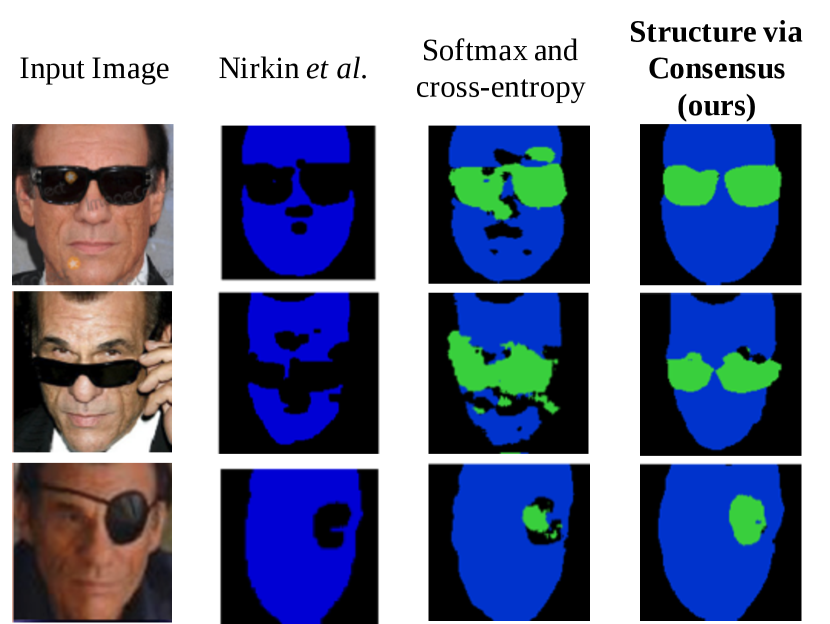
Figure 1: Structure via Consensus. From left to right: the input image; result by [56]; our model with a pixel-wise loss; our proposed method. Previous methods predict only face (blue) vs. background (black), while ours yields separate predictions for occlusions (green) and background (black). Our loss enforces smoothness over objects covering the face via consensus constraint.

While state-of-the-art methods emphasize developing sophisticated architectures (e.g., two-stage networks with recurrent models [47]) or a complex face augmenter to simulate occlusions [56], or rather employ adversarial training [58], we take an alternative path towards robust face segmentation and parsing. Our method builds on an important observation related to the assumption of the independence of pixel-wise predictions. Despite the significance of the aforementioned tasks, current methods overlook the regular structure present in nature and simply optimize for a cost that does not explicitly back-propagate any smoothness into the network parameters. This issue is particularly important for objects and faces, which have a well-defined and continuous (non-sparse) structure.

Fig. 1 shows the advantage of the proposed method on a few samples drawn from the validation set tested on unseen subjects. While publicly available state-of-the-art models [56] perform face segmentation, they do so with very sparse and noncontinuous predictions and by modeling two classes only (face, non-face). In contrast, by virtue of our method, we can separate occlusions from background, and more importantly, arrive at much more stable predictions that are hard to attain with a pixel-wise loss.

As also noted by [35, 28, 46], training a network with pixel-wise softmax and cross-entropy for structured prediction makes the strong and too-simplistic assumption that pixel predictions are independent and identically distributed (i.i.d.). We take inspiration from the Gestalt laws [38]—particularly the ones of proximity (close pixels shall be perceived as a group), closure (pixels shall be grouped into complete figures), good continuation (objects often minimize discontinuity)—and in response to the previous too-simplistic assumption, we make the following contributions which propose: (1) factorizing out occlusions by means of the difference between the complete face shape, attained through a strong prior robustly computed via 3D projections [8, 52], and the output of a preexistent yet error-prone face segmentation network; (2) leveraging the connected components of the objects factorized before, using them as constraints to formulate a new loss function that still performs dense classification, yet enforces structure in the network by consensus learning; (3) finally showing that our approach is a generic tool for face parsing problems up to three classes, thereby reporting promising results in face parsing benchmarks [7, 33]. As an additional contribution, we have released our models and the related code.

The remainder of this paper is organized as follows. Section 2 discusses related work, Section 3 explains our method, Section 4 reports the experimental evaluation, and Section 5 abstracts our findings along with future work.

2 Related Work

Face segmentation. Recent work on face segmentation used a two-stream network [66] to predict a pixel-wise face segmentation mask. The system is fully supervised using pixel-wise segmentation masks obtained by preexisting data sets [26] or by additional semiautomatic manual efforts. Notably, [66] is trained with pixel-wise softmax+cross-entropy, and in order to enforce regularization in the predicted mask, the method uses a conditional random field (CRF) as a post-processing step. Importantly, CRFs have been already used in generic object segmentation and CNNs [83, 84]. Adversarial learning has been used too for segmentation in [50]. Unlike all these methods, ours presents key differences in the way smoothness is propagated in the network. Similar to [66], Nirkin et al. [56] trained a simple fully convolutional net (FCN [49]) for binary face segmentation using a semi-supervised tool to support manual segmentation of faces in videos; in our method we transfer knowledge from the weights of [56], yet we demonstrate that by using our method we can learn from their mistakes and improve the model. Finally, Wang et al. [75] exploited temporal constraints and recurrent models for face parsing and segmentation in video sequences and proposing a differentiable loss to maximize intersection over union (IoU) [62]. Other works extended the face segmentation problem to fine-grained face parsing [71, 30, 44].

Semantic segmentation. Generic semantic segmentation has been an interesting topic in computer vision for a long time—starting with the seminal work using CRFs [6, 72] and graph cut [4, 5]. CRFs impose consistency across pixels, assessing different affinity measures and solving the optimization through a message-passing algorithm [65]. They have been successfully and widely used in face parsing applications also [33, 48]. Recently, they began to be used as a post-processing step [66, 48, 11] with convolutional networks and later on expressed as recurrent neural networks [83]. Super-pixels have also been employed to ease the segmentation process [19, 33], though recently, the field was revolutionized with end-to-end training of FCNs, [49] optimized simply by extending a classification loss [39] to each pixel independently. After [49], there has been extensive progress in deep semantic segmentation— mainly improving convolution to allow for wider receptive fields with its atrous (dilated) version [79, 80], different spatial pooling mechanisms, or more sophisticated architectures [41, 61, 31, 43, 11, 12].

Structure modeling. Modeling structure in computer vision dates back to perceptual organization [54, 67, 16, 15, 17, 14] and to the more general idea of describing objects with a few parts, advocating for frugality [3] in the shape description. Lately, with modern deep-learning, in addition to the aforementioned CRF formulation, all those concepts have faded away in the community—with some exceptions [74, 35]—and instead adversarial training [50, 27, 63, 28] has been used to impose structure in the prediction forcing the output distribution to match the distribution of ground-truth annotations. Other attempts incorporate boundary cues in the training process [1, 9] or pixel-wise affinity [2]; others [30] used a CNN cascade guided by landmark positions. For an in-depth discussion on structured prediction, we refer to [57].

3 Face Parsing with Consensus Learning

Our objective is to robustly learn a nonlinear function $\phi$ parametrized by the weights of a convolutional neural network that maps pixel image intensities $\mathbf{I}\in\mathbb{R}^{3{\mkern-2.0mu\times\mkern-2.0mu}H{\mkern-2.0mu\times\mkern-2.0mu}W}$ to a mask that represents per-pixel semantic label probabilities of the face $\mathbf{y}\in\mathbb{R}^{K{\mkern-2.0mu\times\mkern-2.0mu}H{\mkern-2.0mu\times\mkern-2.0mu}W}$. More formally, we aim to optimize $\phi(\mathbf{I})$ so that it maps $\phi:\mathbb{R}^{3{\mkern-2.0mu\times\mkern-2.0mu}H{\mkern-2.0mu\times\mkern-2.0mu}W}\rightarrow\mathbb{R}^{K{\mkern-2.0mu\times\mkern-2.0mu}H{\mkern-2.0mu\times\mkern-2.0mu}W}$ where $K$ is the number of classes considered in our problem. Importantly, in the learning of $\phi(\cdot)$, while we minimize the expected cost across the training set, we need to enforce a mechanism that incorporates structure through smoothness. At test-time, like current practice, we obtain a final, hard-prediction as $\mathbf{y}^{\prime}\doteq\operatorname{arg\,max}_{k}\phi(\mathbf{I})$ and $\mathbf{y}^{\prime}\in\mathbb{R}^{1{\mkern-2.0mu\times\mkern-2.0mu}H{\mkern-2.0mu\times\mkern-2.0mu}W}$.

The following sections discuss how to obtain some external constraints for enforcing smoothness during the training, though later on we show that our method can be easily employed for the generic face parsing task. We do so by means of transferring knowledge from an existing network and using a strong prior given by 3D face projection to factorize out occluding blobs (Section 3.1). Those blobs are then used to develop a novel loss function that instills structure via consensus learning (Section 3.2).

3.1 Face Segmentation Transfer

Transfer data. Unlike [66] that took advantage of an existing yet small labeled set, or [56] that developed tools to assist the manual labeling, we use facial images from the CASIA WebFaces [78], VGG Faces [59] and MS-Celeb-1M [24] to harvest occlusions in-the-wild without any human effort. We argue that manually annotating them pixel-wise is a painstaking effort and practically infeasible. To pre-train our model, we used $539,960$ training images and $58,306$ validation images without overlapping subjects. In the following sections we explain how we coped with the ambiguous and noisy synthesized pseudo-labels.

Factorizing out occlusions. We express the occlusion appearing in a face image $\mathbf{I}$ as the residual $\bm{\rho}$ obtained from the difference between the full face contour mask $\mathbf{f}$ and the face segmentation mask $\mathbf{f}^{occ}$ provided by [56]. More formally, given $\mathbf{I}$ we further segment it as:

$$\bm{\rho}=\left[\mathbf{f}-\mathbf{f}^{occ}\right]_{+},\quad\operatorname{where}\left[\cdot\right]_{+}=\operatorname{max}\big{(}0,\cdot\big{)}.$$ (1)

Eq. 1 serves to factorize the occlusions out from the background. The mask $\mathbf{f}$ is expressed as the convex hull of the full face shape predicted by projecting onto the image a generic face shape via 3D perspective projection [52] computed using the robust method mentioned in [8]. Note that since we are interested in the facial outer contour, [8] fits our needs since it favors robustness to precision—which is especially useful in the presence of occlusions. This is easily implemented by obtaining the predicted pose $\operatorname{K}[\operatorname{R}|\operatorname{t}]$ and projecting 64 vertices onto the image corresponding to the 3D contour of the face (jawlines plus forehead). Then, $\mathbf{f}$ is efficiently computed finding the simplex of the convex-hull and probing to find if a matrix index $s=(i,j)$ of $\mathbf{f}$ is outside the hull, where $s$ runs over all the pixels in an image. By construction, the residual takes values in $\{-1,0,+1\}$ and is then truncated to $\{0,1\}$ as stated in Eq. 1 to remove possibly ambiguous labels.

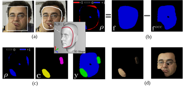
Figure 2: Factorizing out occlusions. (a) We use face detection and a strong prior provided by the projection of a 3D facial shape to get the full face mask; (b) The initial $\bm{\rho}$ residual is expressed as the difference between the full and the segmentation mask; (c) $\bm{\rho}$ is refined and its connected components $\mathbf{C}$ estimated; (d) Label $\mathbf{y}$ is obtained from $\mathbf{C}$ to decouple the occlusions from the face.

The residual then undergoes a series of morphological operations to amplify the occlusions, since, for example, in face completion applications [42, 40] over-segmentation of occlusions is preferable over under-segmentation. The final $\bm{\rho}$ is obtained by applying an erode operator twice with rectangular kernels of size $25{\mkern-2.0mu\times\mkern-2.0mu}7$ and a dilation operation with elliptical kernel of size $45{\mkern-2.0mu\times\mkern-2.0mu}45$. The values are chosen to be conservative with respect to the occlusions: in case the teacher network undersegments occlusions, the rationale was to amplify the occlusions over the face regions. Finally, the connected components are estimated from the residual to identify main blobs or objects on the face. By merging the output of the face segmentation network $\mathbf{f}^{occ}$ and the labels provided by the connected components, the method yields a pseudo-ground-truth mask $\mathbf{C}(\mathbf{I})\in\mathbb{R}^{1{\mkern-2.0mu\times\mkern-2.0mu}H{\mkern-2.0mu\times\mkern-2.0mu}W}$, where $\mathbf{C}$ takes values in $\big{\{}0,\ldots,N_{C}\big{\}}$. Note that, $N_{C}$ is not constant since the number of blobs—i.e., connected components—varies across images; yet by construction, we have that the pixel-wise semantic labels $\mathbf{y}$ are defined as:

$$\forall s,\quad\mathbf{y}(s)=\begin{cases}s\sim\operatorname{background},&\text{if}~{}\mathbf{C}(s)=0,\\ s\sim\operatorname{face},&\text{if}~{}\mathbf{C}(s)=1,\\ s\sim\operatorname{occlusion},&\text{if}~{}\mathbf{C}(s)\geq 2.\end{cases}$$ (2)

The entire process is summarized in Fig. 2.

3.2 Enforcing Structure via Consensus Learning

Network structure. We employ a simple network based on a fully convolutional encoder-decoder [64] taking as input $128{\mkern-2.0mu\times\mkern-2.0mu}128$ RGB images. We note here that the goal is not having a state-of-the-art architecture but to prove the effect of our regularization on the smoothness of the masks. The network uses recurrent applications of a basic building block of Conv–Elu–BatchNorm [13]. The model has two encoding branches: a first encoding branch increases the depth while decreasing spatial dimension up to $256{\mkern-2.0mu\times\mkern-2.0mu}32{\mkern-2.0mu\times\mkern-2.0mu}32$. The second sub-encoder refines the feature maps of the first encoder focusing the attention on a wider part of the input face, using two blocks with dilated convolutions [79]. The feature maps of the two encoders are concatenated together. The decoder maps back to the input spatial dimension using efficient sub-pixel convolution [69] with upscaling ratio of two to upscale the feature maps. Importantly, a final pixel in the classification layer has a receptive field in the input image of $121$ pixels, hence it almost covers the entire face.

A critique of pixel-wise loss functions. The general recipe for semantic segmentation boils down to transforming an image $\mathbf{I}$ using a network $\phi$ that generates a $K{\mkern-2.0mu\times\mkern-2.0mu}H{\mkern-2.0mu\times\mkern-2.0mu}W$ tensor of probabilities $\mathbf{p}$ to maximize the conditioned probability given the ground-truth mask $\mathbf{y}$ with size $1{\mkern-2.0mu\times\mkern-2.0mu}H{\mkern-2.0mu\times\mkern-2.0mu}W$. The network output is expressed as a set of multinoulli distributions, where each pixel prediction $s\sim\operatorname{Cat}\big{(}K,\mathbf{p}(s)\big{)}$. The fitting to the mask labels is implemented with pixel-wise softmax plus cross-entropy, finally averaged over the final tensor. This introduces a strong assumption: all the final generated pixels in the mask behave as independent and identically distributed (i.i.d.) random variables, which violates the regular structures implicitly present in nature [28]. Defining a pixel location as $s$, the expected loss across all pixel’s image $\mathbb{E}[\ell(\cdot)]$ is eventually:

$$\frac{1}{HW}\sum_{s=1}^{HW}\ell(s)=\frac{1}{HW}\sum_{s=1}^{HW}\mathcal{H}\Big{(}\mathbf{p}(s),\mathbf{y}(s)\Big{)}=\\ =-\frac{1}{HW}\sum_{s=1}^{HW}\mathbf{y}(s)\log\big{(}\mathbf{p}(s)\big{)}~{},$$ (3)

where $\mathcal{H}$ indicates the cross-entropy between the predicted softmax probability $\mathbf{p}(s)$ and $\mathbf{y}(s)$ is one-hot encoding of the class membership at a pixel $s$. More analytically:

$$\mathbb{E}[\ell(\cdot)]=-\frac{1}{HW}\sum_{s\in\mathbf{y}}\log\Bigg{(}\frac{e^{\mathbf{W}_{(k^{\star},s)}\mathbf{x}_{(k^{\star},s)}^{T}}}{\sum_{k=1}^{K}e^{\mathbf{W}_{(k,s)}\mathbf{x}_{(k,s)}^{T}}}\Bigg{)},$$ (4)

where $k$ runs over the classes, $k^{\star}$ selects the ground-truth class index based on $\mathbf{y}$, and $s$ runs on all the pixels. $\mathbf{W}$ represents the final classification convolutional layer mapping to the label space and $\mathbf{x}$ the activation before $\mathbf{W}$.

Eq. 4 assumes that the prediction at a given pixel is not regularized by the structure present in the input, and hence it suggests improvement by incorporating smoothness constraints. Although each pixel prediction in $\mathbf{x}$ has some knowledge of the neighbour pixels in the input image, given the recurrent application of convolutions, this is not enough to avoid predicting pixels independently, even in the dilated case [79, 80] allowing for large receptive fields as in our model. Despite the recent progress in semantic segmentation [12], the aforementioned issue is not yet fully addressed in the face domain. Eq. 4 is also often used in applications such as face segmentation, face parsing or occlusion detection, and in many cases where the network has to densely label pixels. The problem of returning sparse predictions is especially important on faces, since these exhibit a very regular structure. The same is true for occlusion covering the face: obstructing objects covering the face are rarely composed of sparse tiny parts, yet rather show up with continuous shapes.

Preliminaries. The above problem calls for a solution regarding the independent assumption of the predictions in Eq. 4. Unlike [66, 56] that couple the background and occlusion classes together, we define face segmentation as a three-class problem ($K=3$) aiming to classify background $\mathbf{B}$, face $\mathbf{F}$ and occlusion $\mathbf{O}$. Additionally, following Section 3.1, we allow for occlusions to be modeled as a variable set of blobs over the face $\mathcal{O}=\{\mathbf{O}_{1},\ldots,\mathbf{O}_{n}\}$. In spite of this, Eq. 3 can be rewritten as:

$$\frac{1}{|\mathbf{F}|}\sum_{s\in\mathbf{F}}\ell(s)+\frac{1}{|\mathbf{B}|}\sum_{s\in\mathbf{B}}\ell(s)+\frac{1}{|\mathcal{O}|}\sum_{\mathbf{O}\in\mathcal{O}}\Bigg{(}\frac{1}{|\mathbf{O}|}\sum_{s\in\mathbf{O}}\ell(s)\Bigg{)},$$ (5)

where $\ell(s)$ corresponds to the softmax plus cross-entropy loss at a pixel $s$, that runs over all the pixels in each blob, and $|\cdot|$ counts the pixels of a blob. Eq. 5 is identical to Eq. 3, with the only difference being that the spatial frequency of each component is marginalized out, or in other terms, having the same weights for all blobs irrespective of their size. Next, we explain how to enforce smoothness in our training process.

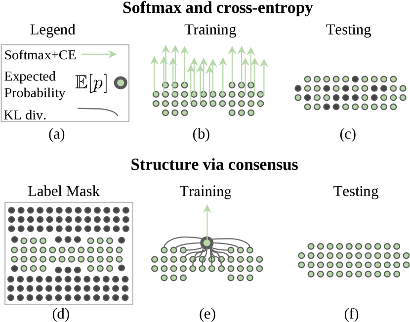
Figure 3: Intuition behind our loss. (a) legend; (b) regular training proceeds pixel-wise, independently and enforces densely each pixel to fit the label (no notion of smoothness of the object); (c) this leads to sparse prediction at test time for unseen objects; (d) pixel-wise labels for an image; (e) we force the expected prediction in a blob $\mathbb{E}[\mathbf{p}]$ to the label, yet ensure no deviation of each pixel from the average; (f) the network is better regularized for segmenting with less sparse predictions.

Enforcing structure in each blob. The core idea behind our method is shown in Fig. 3. We define the expected probability $\mathbb{E}[{\mathbf{p}}]$ on a blob $\mathbf{c}$ as:

$$\widehat{\mathbf{p}}_{\mathbf{c}}\doteq\frac{1}{|\mathbf{c}|}\sum_{s\in\mathbf{c}}\mathbf{p}(s)=\frac{1}{|\mathbf{c}|}\sum_{s\in\mathbf{c}}\Bigg{(}\frac{e^{\mathbf{W}_{(k^{\star},s)}\mathbf{x}_{(k^{\star},s)}^{T}}}{\sum_{k=1}^{K}e^{\mathbf{W}_{(k,s)}\mathbf{x}_{(k,s)}^{T}}}\Bigg{)},$$ (6)

that corresponds to the average conditioned probability over all the pixels of the blob $\mathbf{c}$. Note that the values in Eq. 6 remain positive and the mass of $\widehat{\mathbf{p}}_{\mathbf{c}}$ sums up to one. Then, we can augment Eq. 3 in the following way: given a blob on the mask we can define the loss on the blob as

$$\underbrace{\alpha\cdot D_{KL}\big{(}\mathbf{y}~{}||~{}\widehat{\mathbf{p}}_{\mathbf{c}}\big{)}}_{\text{1st order; matches the class label}}+\underbrace{\beta\cdot\frac{1}{|\mathbf{c}|}\sum_{s\in\mathbf{c}}D_{KL}\big{(}\widehat{\mathbf{p}}_{\mathbf{c}}~{}||~{}\mathbf{p}(s)\big{)}}_{\text{2nd order; ensures no deviation}},$$ (7)

where $\alpha$, $\beta$ are two constant parameters controlling the trade-off between matching the labels and ensuring consensus and $D_{KL}$ denotes the Kullback-Leibler divergence. Following the notation of  Section 3.1, and putting this all together, indicating all the the blobs (background $\mathbf{B}$, face $\mathbf{F}$, occlusions $\mathcal{O}$) as $\mathbf{C}$, our method finally optimizes:

$$\frac{1}{|N_{C}|}\sum_{\mathbf{c}\in\mathbf{C}}\Bigg{[}\alpha\,D_{KL}\big{(}\mathbf{y}~{}||~{}\widehat{\mathbf{p}}_{\mathbf{c}}\big{)}+\frac{\beta}{|\mathbf{c}|}\sum_{s\in\mathbf{c}}D_{KL}\big{(}\widehat{\mathbf{p}}_{\mathbf{c}}~{}||~{}\mathbf{p}(s)\big{)}\Bigg{]}.$$ (8)

Note that although here we apply our formulation specifically to face segmentation/occlusion detection, if the method is provided with a set of blobs, then it can be applied more broadly. Section 4 shows how to easily obtain blobs from the available labels in benchmarks for a generalization to face parsing with a small number of classes.

3.3 Interpretations

Eq. 8 can be interpreted as follows: given a blob on the mask $\mathbf{c}$, we enforce that the average of the predictions over the blob has to match the class label $D_{KL}\big{(}\mathbf{y}~{}||~{}\widehat{\mathbf{p}}_{\mathbf{c}}\big{)}$—as a sort of first-order momentum—plus a second term ensures that all pixel-wise probabilities inside the blob are close to its average, i.e., $\sum_{s\in\mathbf{c}}D_{KL}\big{(}\widehat{\mathbf{p}}_{\mathbf{c}}~{}||~{}\mathbf{p}(s)\big{)}$. We treat each blob as a whole using the first term and we enforce smoothness using the regularization of the second term: unlike the baseline, our loss connects all the pixel predictions in a blob with the average prediction, defining implicit inter-dependencies as a sort of regularizer. As a cross-topic parallelism, it may be useful to the reader to know that a similar smoothness regularization has been proposed recently to induce smoothness to cope with adversarial attacks [34].

Implementation. In the first term, what is actually implemented as $D_{KL}$ is the negative log-likelihood of the ground-truth probability from $\widehat{\mathbf{p}}_{\mathbf{c}}$. This can still be viewed as KL div. since this latter reduces to cross-entropy given that $D_{KL}\big{(}\mathbf{y}~{}||~{}\widehat{\mathbf{p}}_{\mathbf{c}}\big{)}\doteq\mathcal{H}\big{(}\mathbf{y},\widehat{\mathbf{p}}_{\mathbf{c}}\big{)}-\mathcal{H}\big{(}\mathbf{y}\big{)}$, and, $\mathbf{y}$, the target distribution, is a one-hot encoding, thus with entropy equal to zero. Hence, KL div. is equal to cross-entropy in this case. The second term in Eq. 8 is simply implemented as KL div. between two discrete distributions. In this sense, Eq. 8 keeps an elegant consistency across its two terms, without requiring the system for external CRF post-processing or additional parameters to perform adversarial training.

Interpretation as a generalization of Eq. 4. Additionally, the proposed formulation can be seen as a generalization of Eq. 4. A pixel-wise loss coincides with a boundary case of our loss when all the blobs collapse down to each pixel. In this case, each pixel matches the class label—first term in Eq. 8—and the second term collapses to zero, since, by definition, a pixel is consistent to itself.

Connection to CRFs. Our formulation shares some similarities with seminal CRFs [6, 72, 48] and graph cut [4, 5] for semantic segmentation. At first sight the two terms in Eq. 7 are reminiscent of minimizing the energy of a function $\phi$ as $E_{data}(\phi)+E_{smooth}(\phi)$, as proposed in [5]. Though the CRF has already been used in conjunction with a ConvNet (e.g., [83, 11]), we do share the core philosophy with novel traits; unlike [5], our “unary potential” is not defined on single pixels but on the expected probability over the shape, and our “pair-wise potential” is not defined on pairs of adjacent pixels [5] or fully connected [11], yet is constrained by components with characteristic shapes. We note here that in our case $\phi$ is parameterized by the filters of a ConvNet. Finally, we acknowledge that CRFs captures long range interactions via a fully-connected graphical structure, in contrast, the proposed loss only captures constraints within neighborhoods; though, the “neighborhood” in our case can be small or large depending on the label masks or connected components mined in Section 3.1. In light of this, our formulation still exhibits innovative traits.

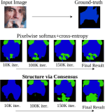
(a) Training progress

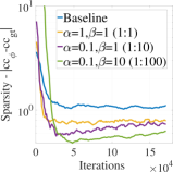
(b) $|\operatorname{cc}_{\phi}-\operatorname{cc}_{gt}|$

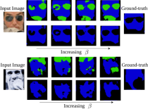
(c) Increasing $\beta$ reduces sparsity

Figure 4: More regular, smooth structure learned; (a) As the training progresses, our method learns more regular, smooth structure which yields a more regular mask when compared to the pixel-wise baseline (sample from the COFW test set); (b) less sparsity is confirmed by visualization of the error in the number of connected components between the predicted $\operatorname{cc}_{\phi}$ and annotated mask $\operatorname{cc}_{gt}$. A higher weight on $\beta$ greatly decreases the sparsity of the masks (c) this effect is confirmed when inspecting qualitative samples from the COFW test set.

4 Experimental Evaluation

We report results of ablation study or experiments that motivated our choices, along with state-of-the-art evaluations on benchmarks for face segmentation, occlusion detection and face parsing. Our approach surpasses previous methods by wide margins on the COFW (Caltech Occluded Faces in the Wild) [7] and shows comparable results on the Part Labels set [33] despite using a lightweight model.

4.1 Implementation Details

Face preprocessing. Following [47], we used a minimalist face preprocessing, simply applying a face detector [77] and using the adjusted square box to crop and resize each face and its corresponding label to $128{\mkern-2.0mu\times\mkern-2.0mu}128$ pixels. On Part Labels, faces are aligned thus we just resize them to $128$p.

Training. To pre-train the network we use the Adam optimizer [37], starting from a learning rate of $\operatorname{1e-3}$ and finishing with $\operatorname{1e-5}$. Pseudo-labels are provided following Section 3.1. A scheduler checks the pixel-wise average recall across classes on the validation and decreases the learning by $\operatorname{1e-1}$ when the above metric plateaus. All the models are trained with a batch size of $128$. When fine-tuning on COFW, we apply our face segmentation transfer (Section 3.1) to identify the main blobs without applying the morphological operations to use the fine-grain human annotated masks. In other tests, we simply treat the separate mask classes as the blobs. On COFW we used a flat learning rate of $\operatorname{1e-5}$, while on Part Labels $\operatorname{1e-4}$. All the models are fine-tuned until convergence reaches saturation on the training set. Important parameters in Eq. 7 are $\alpha$, $\beta$ that are set as $\{10$:$5\}$ in all our experiments, as we found these values to be a good trade-off between enforcing smoothness and fitting the labels to guarantee high accuracy.

4.2 Supporting Experiment

More regular, less scattered structure. Fig. 4a shows qualitatively the difference in the prediction between the baseline and learning with structure via consensus on a COFW [7] test sample when performing transfer learning with our loss. The sample is chosen for its difficulty in the face segmentation task (the occlusion appears fragmented—although it is not—and is of similar color to the face, in spite of the fact that it is made by two continuous objects (e.g., hands and microphone). As the training progresses, our method offers more continuous segmentation masks that, in turn, become a better face segmentation, without sparse holes. Our claim is supported by Fig. 4b, showing the average absolute error $\frac{1}{N}\sum_{i}^{N}|\operatorname{cc}_{\phi}-\operatorname{cc}_{gt}|$ between the number of connected components in the ground-truth mask ($cc_{gt}$) and the components dynamically computed on our prediction ($cc_{\phi}$) at every iteration. The error is averaged across all the testing samples and provides a valuable understanding of the sparsity of the prediction and confirms that increasing our smooth term $\beta$ in Eq. 8 induces a significant less sparse output. Fig. 4b shows the trend of the sparsity error measure as the training evolves for different $\beta$ values. Additional qualitative samples in Fig. 4c further support our hypothesis.

Input, Label Mask   Nirkin et al. [56]      Baseline       Ours

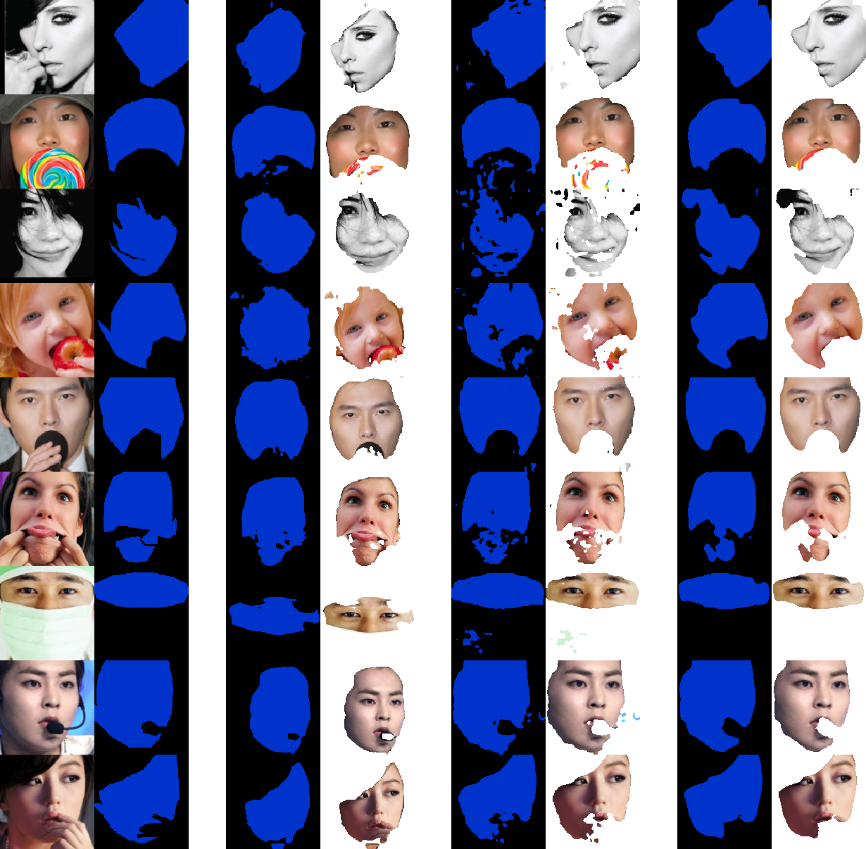
Figure 5: Qualitative samples from the COFW set. Input image and its ground-truth mask; results by Nirkin et al. [56]; baseline with pixel-wise loss; our result. The faces are masked to remove occlusions according to each method. Additional results in the supplementary material in Fig. 8.

4.3 Caltech Occluded Faces in the Wild

Method	IOU${}_{\text{\emph{face}}}$	acc.	rec${}_{\text{\emph{face}}}$	rec${}_{\text{\emph{all}}}$	spars.	fps
Struct. Forest [32]	—	83.9	—	88.6	—	—
RPP [76]	72.4	—	—	—	—	0.03
SAPM [20]	83.5	88.6	87.1	—	—	—
Liu et al. [48]	72.9	79.8	89.9	77.9	—	0.29
Saito et al. [66] +GraphCut	83.9	88.7	92.7	—	—	43.2
Nirkin et al. [56]	81.6	87.4	93.3	—	—	48.6
Nirkin et al. [56] +Occ. Aug.	83.7	88.8	94.1	87.4	—	48.6
Softmax+CE +Scratch	76.8	83.7	86.9	82.6	3.5	300
Softmax+CE +Transf.	84.5	89.4	93.3	88.1	1.0	300
Softmax+CE +Transf.+f.t.	84.1	89.4	90.3	89.1	3.8	300
Struct. via con. +Transf.+f.t.	85.7	90.4	92.5	89.7	1.6	300
Struct. via con. +Transf.+f.t.+reg.	87.0	91.3	92.4	90.9	0.8	300

Table 1: COFW set. Occlusion segmentation results.

Comparison with the state-of-the-art. We use the COFW set [7] for proving the effectiveness of our method. COFW consists of $500$ labeled images for training and $507$ for testing. Labels consist of binary masks. Table 1 reports our results compared to the state-of-the-art, along with ablation study to motivate our choices. The table reports figures for face IOU intersection over union (or Jaccard index), pixel accuracy (acc.), pixel-wise recall of the face class (rec${}_{\text{\emph{face}}}$), average pixel-wise recall across all classes (rec${}_{\text{\emph{all}}})$ face and non-face, our measure of sparsity ($\frac{1}{N}\sum_{i}^{N}|\operatorname{cc}_{\phi}-\operatorname{cc}_{gt}|$) and fps (frames per second). When we test our method we simply merge the responses from the occlusion class and background class as a single non-face class. Following previous work [32, 76, 20], we report the metrics in the face box provided with COFW. Given the small size of COFW, it is challenging to fine-tune a deep model. To prove this point, and, more importantly, to motivate Section 3.1, we train from random weights (+Scratch). Since we are updating the weights very slowly, the model is able to learn, yet reaches a result that is too distant from the state-of-the-art. For this reason, previous methods [66, 56] employed other labeled sets [33] or built semiautomatic annotation tools [56] to attain some sort of transfer learning. Similar to them, we perform transfer learning, yet unlike them, we transfer knowledge from [56] as explained in Section 3.1. Results in Table 1 (+Transf.) support our face segmentation transfer. Our method is able to outperform the teacher network [56]. Additionally, if we combine all our novelties and further fine-tune on COFW, we obtain an additional positive gap with respect to the state-of-the-art (Struct. via con. +Transf.+F.t.+reg.). Our method reduces the overall error-rate by 27.7% for the metric rec${}_{\text{\emph{all}}}$. As a final note, since we are using a lightweight encoder-decoder, unlike [66], our smoothness constraint is enforced at training time only. Our inference time is remarkable: on average a forward pass takes $3.1$ ms yielding more than $300$ predicted masks per second (fps).

Ablation study. The effect of learning with “structure via consensus” is shown in Table 1 and is compared to the softmax+CE. While fine-tuning with the pixel-wise loss increases sparsity on the masks (1.0 $\rightarrow$ 3.8) and actually reduces performance; on the contrary, by enforcing smoothness with our loss, we are able to better generalize to the test set, to improve over the transfer learning and to keep a lower sparsity (1.6). Further gain is obtained by regularizing the model with dropout and flip augmentation (+reg.). A qualitative comparison is shown in Fig. 5, where our method shows more structured masks than the baseline and [56]. Other qualitative samples are shown in Figs. 1, 4a and 4c.

4.4 Part Labels Database

Method	size${}_{\emph{in}}$	No CRF	acc.${}_{\emph{p}}$	acc.${}_{\emph{sp}}$
Gygli et al. [25] — DVN	32	✓	—	92.44
Gygli et al. [25] — FCN baseline	32	✓	—	95.36
Kae et al. [33] — CRF	250	✗	—	93.23
Kae et al. [33] — Glog	250	✗	—	94.95
Liu et al. [48]	250	✗	95.24	—
Liu et al. [47] — RNN	128	✓	95.46	—
Liu et al. [47, 10] — CNN-CRF	128	✗	92.59	—
Saxena et al. (sparse) [68]	250	✓	94.60	95.58
Saxena et al. (dense) [68]	250	✓	94.82	95.63
Zheng et al. [82] — CNN-VAE	250	✓	—	96.59
Tsogkas et al. [73] — CNN	250	✓	—	96.54
Tsogkas et al. [73] — RBM+CRF	250	✗	—	96.97
Lin et al. [44] — FCN+Mask-R-CNN	250	✓	96.71	—
Adversarial Training
FCN — GAN [22]	250	✓	—	95.53
GAN [22]	250	✓	—	95.54
FCN — LSGAN [51]	250	✓	—	95.51
LSGAN [51]	250	✓	—	95.52
FCN — WGAN,GP [23]	250	✓	—	95.59
WGAN,GP [23]	250	✓	—	95.59
FCN — EBGAN [81]	250	✓	—	95.50
EBGAN [81]	250	✓	—	95.52
FCN — LDRSP [58]	250	✓	—	95.87
LDRSP [58]	250	✓	—	96.47
Structure via Consenus (Ours)	128	✓	96.05	96.80
Structure via Consenus (Ours)	250	✓	95.86	96.78

Table 2: Part Labels set. The comparison of pixel and super-pixel accuracies (acc.${}_{\emph{p}}$, acc.${}_{\emph{sp}}$). The input size and usage of smoothness via CRF are emphasized. Best result is in bold, while second best is underlined.

Comparison with the state-of-the-art. Following previous work [33], we employ the funneled version of the set, in which images have already been coarsely aligned. Part Labels is a subset of LFW [26] for face segmentation proposed in [33], and consists of 1,500 training, 500 validation, and 927 testing images. The images are labeled with efficient super-pixel segmentation. The set provides three classes–background, hair/facial-hair and face/neck along with the corresponding super-pixel mapping. We fine-tune our system on the 2,000 train/val images and test on the 927 evaluation faces following the publicly available splits. When fine-tuning, we associate the Part Labels classes with the same semantic class of the transfer learning except for the occlusion class being mapped to the new hair class. To have a thorough comparison with current work, we report both pixel-wise (acc.${}_{\emph{p}}$) and super-pixel-wise accuracies (acc.${}_{\emph{sp}}$). To report the super-pixel accuracy, we select the most frequent predicted label in a super-pixel. Our system reports results on par with the state-of-the-art, noting that in our case we perform direct inference (no CRF ✓), and we are not forcing any smoothness via CRF at test-time. Table 2 shows the state-of-the-art evaluation. We have results similar to Tsogkas et al. [73], yet they use a CRF to smooth out the result. Notably, our approach shows similar numbers when compared with the active research of adversarial training (following the extensive experimentation from [58]), though this latter requires more parameters because of the discriminator. Table 4 reports also the F1-score following the recent work in [44]. Although our method works at a 128p resolution we report results at 250p by up-sampling the predictions with nearest neighbor interpolation.

Ablation Study. In Table 3 we report ablation study showing the impact of our loss: in general pixel accuracy increases with our loss but since these metrics do not take into account class frequencies, we also recorded the IOU per class. Using “structure via consensus” the IOU for hair class goes up from $68.95\%$ to $72.48\%$. The same is reflected in the mean IOU over classes—from $83.65\%$ to $85.74\%$. We repeated the same experiments further regularizing the model with dropout and flip augmentation (+reg.), our loss provided a similar improvement, and, importantly, the boost is consistent in all the metrics. Notably in all these ablations, our method provided less sparse masks when compared to the baseline as reported in Table 3 under the sparsity metric, exhibiting less over-fitting than the baseline. Qualitative results are shown in Fig. 6: our hair segmentation exhibits less fragmented segments and fewer holes than the baseline, yet yielding an excellent face segmentation.

Method	IOU${}_{\text{\emph{hair}}}$	IOU${}_{\text{\emph{bg}}}$	IOU${}_{\text{\emph{face}}}$	IOU${}_{\text{\emph{mean}}}$	recall${}_{\text{\emph{all}}}$	acc.${}_{\emph{p}}$	acc.${}_{\emph{sp}}$	spars.
Baseline	68.95	94.41	87.60	83.65	90.41	94.77	96.15	15.86
Struct. via cons.	72.48	95.17	89.98	85.74	91.26	95.55	96.61	13.66
Baseline +reg.	73.97	95.52	89.81	86.46	92.50	95.77	96.62	3.3
Struct. via cons. +reg.	75.84	95.74	90.62	87.40	93.22	96.05	96.80	3.3

Table 3: Ablation study on Part Labels set. Detailed ablation study on the Part Labels set for the base model and a model with additional regularization (+reg.).

Method	size${}_{\emph{in}}$	F1${}_{\text{\emph{face}}}$	F1${}_{\text{\emph{hair}}}$	F1${}_{\text{\emph{bg}}}$	acc.${}_{\emph{p}}$
Liu et al. [48]	–	93.93	80.70	97.10	95.12
Long et al. [49]	–	92.91	82.69	96.32	94.13
Chen et al. [11]	–	92.54	80.14	95.65	93.44
Chen et al. [9]	–	91.17	78.85	94.95	92.49
Zhou et al. [84]	320	94.10	85.16	96.46	95.28
Liu et al. [47]	128	97.55	83.43	94.37	95.46
Lin et al. [44]	250	95.77	88.31	98.26	96.71
Struct. via cons. (Ours)	128	95.08	86.26	97.82	96.05
Struct. via cons. (Ours)	250	94.74	85.74	97.72	95.86

Table 4: F1-score comparison on Part Labels. Ours is the second best despite using a lightweight model. Numbers from [44]. Best result is in bold, while second best is underlined.

Input, Label Mask                Baseline                Ours

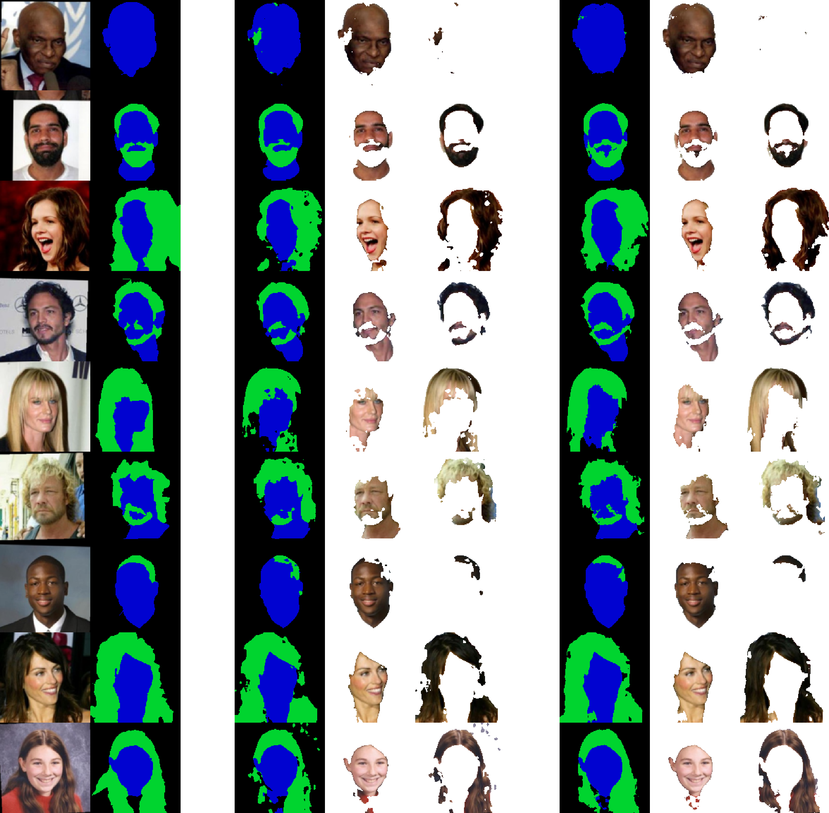
Figure 6: Qualitative results from the Part Labels. Input image and its ground-truth mask; results by the baseline with pixel-wise loss; our result. The faces are masked to decouple the face from the hair. Additional results in the supplementary material in Fig. 9.

5 Conclusions and Future Work

We proposed a novel method for face segmentation, building on the novel concept of learning structure via consensus. Our approach exhibits figures on par or above the state-of-the-art. Our future work is to experiment with Pascal VOC [18] on the generic task of semantic segmentation, thereby porting our loss to work with generic objects. The system is using blobs as a constraint for the consensus, and those are given as input to the system through an automatic, noisy preprocessing step or by some form of human supervision from the annotations. As a more long-term future work, we envision the possibility of learning to cluster pixels of objects in an unsupervised fashion.

Acknowledgements. This research is based upon work supported by the Office of the Director of National Intelligence (ODNI), Intelligence Advanced Research Projects Activity (IARPA), via IARPA R&D Contract No. 2017-17020200005. The views and conclusions contained herein are those of the authors and should not be interpreted as necessarily representing the official policies or endorsements, either expressed or implied, of the ODNI, IARPA, or the U.S. Government. The U.S. Government is authorized to reproduce and distribute reprints for Governmental purposes notwithstanding any copyright annotation thereon. The authors would like to thank S. Deutsch, A. Jaiswal, H. Mirzaalian, M. Hussein, L. Spinoulas and all the anonymous reviewers for their helpful discussions.

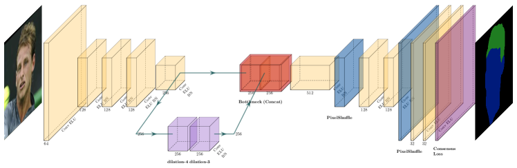
Figure 7: Network structure at a glance. Encoder-decoder used for face segmentation and supervised through structure via consensus.

Appendix A Network Architecture

Architecture Details. Further details of our network architecture are provided in Table 5. Our network is similar to the encoder-decoder framework U-Net [64], but it has some modifications explained below. The input resolution is $128{\mkern-2.0mu\times\mkern-2.0mu}128$, though our model can work also with other resolutions since it is fully convolutional. The resolution is decreased only with striding without any pooling layer. The basic block of the network consists of ReflectionPad2, Convolution, ELU [13] and Batch Normalization. The first encoder downsamples the input up to $32{\mkern-2.0mu\times\mkern-2.0mu}32$ to preserve some spatial information, with a depth of 256 (layer id 19 referring to Table 5); then other convolutional layers with dilation set to 4 and 3 in a sub-encoder refine the feature maps to capture a more global scale (layer id 27 referring to Table 5). In Table 5, if not specified, convolution is computed with dilation equal to 1. The final feature maps are concatenated together for a final bottleneck feature map with dimensionality $512{\mkern-2.0mu\times\mkern-2.0mu}32{\mkern-2.0mu\times\mkern-2.0mu}32$. The convolutional filters are initialized with the method described in  [21]. The decoder part takes the bottleneck feature maps as input and upscales it back to the input dimension. We used efficient sub-pixel convolution with ratio equal to 2 applied two times in the decoder to do this upscaling, since sub-pixel convolution has been shown to work well in super-resolution applications. We used Pytorch [60] to develop the network and sub-pixel convolution has been implemented via PixelShuffling. The entire encoder-decoder has 4,524,323 parameters. The network is supervised either with 2D softmax normalization and cross-entropy or by using our novel “structure via consensus” method. The final network structure is displayed at a glance in Fig. 7 using [29].

ID	Layer (type)	Output Shape ($B{\mkern-2.0mu\times\mkern-2.0mu}C{\mkern-2.0mu\times\mkern-2.0mu}H{\mkern-2.0mu\times\mkern-2.0mu}W$)	Param. Size
Encoder $\downarrow$
1	ReflectionPad2d	[64, 3, 130, 130]	—
2	Conv2d	[64, 64, 128, 128]	1,792
3	ELU	[64, 64, 128, 128]	—
4	ReflectionPad2d	[64, 64, 130, 130]	—
5	Conv2d	[64, 128, 64, 64]	73,856
6	ELU	[64, 128, 64, 64]	—
7	BatchNorm2d	[64, 128, 64, 64]	256
8	ReflectionPad2d	[64, 128, 66, 66]	—
9	Conv2d	[64, 128, 64, 64]	147,584
10	ELU	[64, 128, 64, 64]	—
11	BatchNorm2d-	[64, 128, 64, 64]	256
12	ReflectionPad2d-	[64, 128, 66, 66]	—
13	Conv2d	[64, 128, 64, 64]	147,584
14	ELU	[64, 128, 64, 64]	—
15	BatchNorm2d-	[64, 128, 64, 64]	256
16	ReflectionPad2d	[64, 128, 66, 66]	—
17	Conv2d	[64, 256, 32, 32]	295,168
18	ELU	[64, 256, 32, 32]	—
19	BatchNorm2d	[64, 256, 32, 32]	512
Sub-encoder $\downarrow$
20	ReflectionPad2d	[64, 256, 40, 40]	—
21	Conv2d (dilation=4)	[64, 256, 32, 32]	590,080
22	ELU	[64, 256, 32, 32]	—
23	BatchNorm2d	[64, 256, 32, 32]	512
24	ReflectionPad2d	[64, 256, 38, 38]	—
25	Conv2d (dilation=3)	[64, 256, 32, 32]	590,080
26	ELU	[64, 256, 32, 32]	—
27	BatchNorm2d	[64, 256, 32, 32]	512
Concat feature maps 19 and 27
Decoder $\uparrow$
28	ReflectionPad2d	[64, 512, 34, 34]	—
29	Conv2d	[64, 512, 32, 32]	2,359,808
30	ELU	[64, 512, 32, 32]	—
31	BatchNorm2d	[64, 512, 32, 32]	1,024
32	PixelShuffle (${\mkern-2.0mu\times\mkern-2.0mu}2$)	[64, 128, 64, 64]	—
33	ReflectionPad2d	[64, 128, 66, 66]	—
34	Conv2d	[64, 128, 64, 64]	147,584
35	ELU	[64, 128, 64, 64]	—
36	BatchNorm2d	[64, 128, 64, 64]	256
37	ReflectionPad2d	[64, 128, 66, 66]	—
38	Conv2d	[64, 128, 64, 64]	147,584
39	ELU	[64, 128, 64, 64]	—
40	BatchNorm2d	[64, 128, 64, 64]	256
41	PixelShuffle (${\mkern-2.0mu\times\mkern-2.0mu}2$)	[64, 32, 128, 128]	—
42	ReflectionPad2d	[64, 32, 130, 130]	—
43	Conv2d	[64, 32, 128, 128]	9,248
44	ELU	[64, 32, 128, 128]	—
45	ReflectionPad2d	[64, 32, 130, 130]	—
46	Conv2d	[64, 32, 128, 128]	9,248
47	ELU	[64, 32, 128, 128]	—
48	Conv2d	[64, 3, 128, 128]	867
		Total # params.	4,524,323

Table 5: Network details. Network layers, output shapes and learnable parameters.

Appendix B Additional Qualitative Results on COFW

We show supplementary results on the Caltech Occluded Face in the Wild data (COFW) [7] in Fig. 8. The figures augment Fig. 5 in the paper to provide further samples. The figures display the input image and its ground-truth mask; the result obtained by Nirkin et al. [56], obtained by aligning the faces as the mentioned in their publicly available code; our baseline with pixel-wise softmax and cross-entropy; our final approach trained with structure via consensus. Fig. 8 show again that even on a larger pool of samples, our method returns less sparse, more continuous occlusion masks for better face segmentation and parsing. As a remark, we get such clean masks, much closer visually to the ground-truth compared to other approaches, yet we do so by still performing pixel-wise inference: we do not use any super-pixel approach at test time nor employ any post-processing step such as CRF, morphological operations etc.

Input, Label    Nirkin et al. [56]    Baseline       Ours  

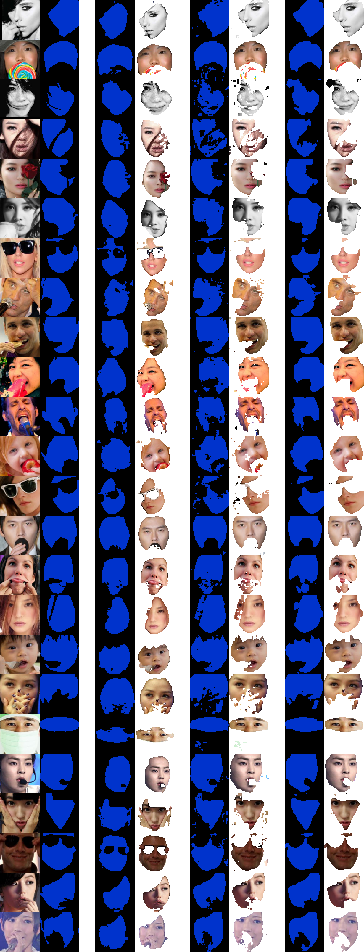
Figure 8: Additional qualitative samples from the COFW. Input image and its ground-truth mask; results by Nirkin et al. [56]; baseline with pixel-wise loss; our result. The faces are masked to remove occlusions according to each method.

Appendix C Additional Qualitative Results
on Part Labels

We show some supplementary qualitative results on the Part Labels database [33] in Fig. 9. On average our masks look more continuous and greatly improve the IoU of the hair class. Fig. 9 reports the input image, the ground-truth annotated mask, the baseline model trained with pixel-wise loss and regularization and our method with regularization. The result of each prediction for each class is used for segmenting part of the face showing the segmentation separately for face and hair. In some cases, the predictions of our model are better than the super-pixel labels (e.g. tenth row).

Input, Label Mask       Baseline          Ours

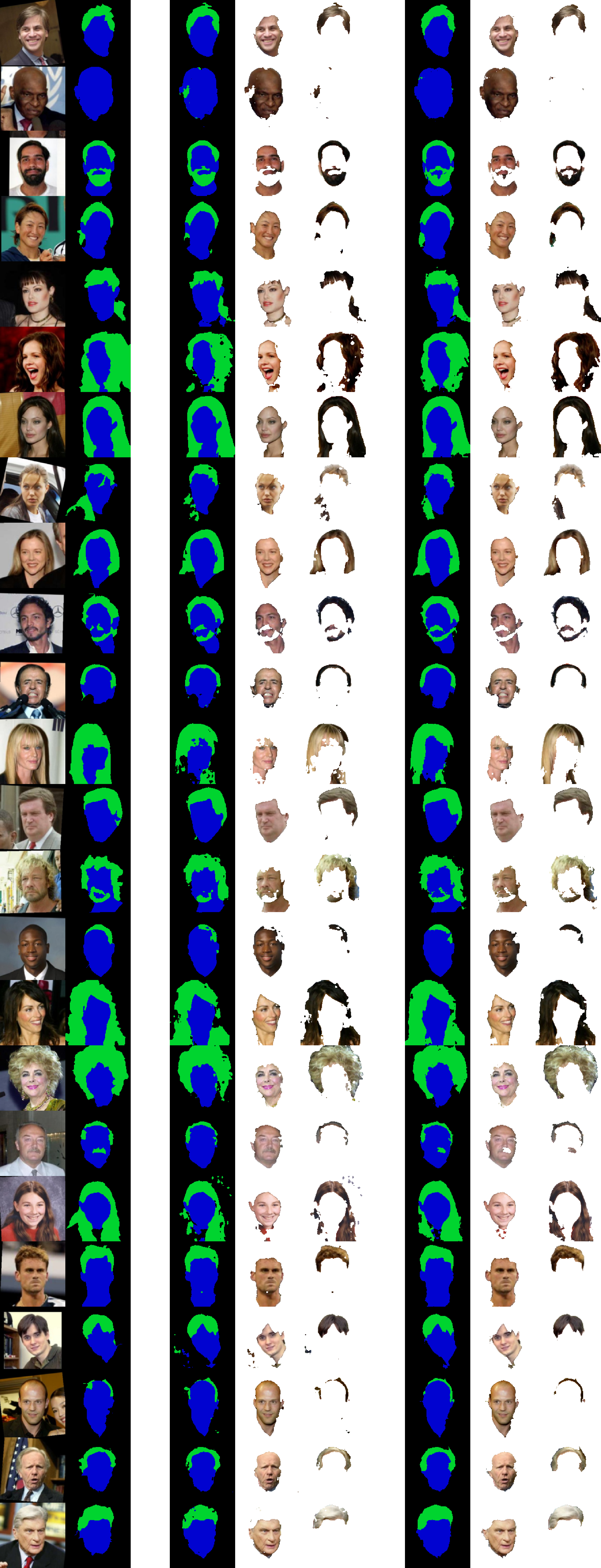
Figure 9: Additional qualitative samples from PartLabel. Input image and its ground-truth mask; results by the baseline with pixel-wise loss; our result. The faces are masked to decouple the face from the hair.

References

- [1] Gedas Bertasius, Jianbo Shi, and Lorenzo Torresani. Semantic segmentation with boundary neural fields. In CVPR, 2016.
- [2] Gedas Bertasius, Lorenzo Torresani, Stella X Yu, and Jianbo Shi. Convolutional random walk networks for semantic image segmentation. In CVPR, 2017.
- [3] Thomas Binford and Jay Tenenbaum. Visual perception by computer. In IEEE Conference on Systems and Control, 1971.
- [4] Yuri Boykov, Olga Veksler, and Ramin Zabih. Fast approximate energy minimization via graph cuts. In ICCV, volume 1, pages 377–384, 1999.
- [5] Yuri Boykov, Olga Veksler, and Ramin Zabih. Fast approximate energy minimization via graph cuts. TPAMI, 23(11):1, 2001.
- [6] Yuri Y Boykov and M-P Jolly. Interactive graph cuts for optimal boundary & region segmentation of objects in nd images. In ICCV, 2001.
- [7] Xavier P Burgos-Artizzu, Pietro Perona, and Piotr Dollár. Robust face landmark estimation under occlusion. In ICCV, pages 1513–1520. IEEE, 2013.
- [8] Feng-ju Chang, Anh Tran, Tal Hassner, Iacopo Masi, Ram Nevatia, and Gérard Medioni. FacePoseNet: Making a case for landmark-free face alignment. In ICCV Workshops, 2017.
- [9] Liang-Chieh Chen, Jonathan T Barron, George Papandreou, Kevin Murphy, and Alan L Yuille. Semantic image segmentation with task-specific edge detection using cnns and a discriminatively trained domain transform. In CVPR, 2016.
- [10] Liang-Chieh Chen, George Papandreou, Iasonas Kokkinos, Kevin Murphy, and Alan L Yuille. Semantic image segmentation with deep convolutional nets and fully connected crfs. In ICLR, 2015.
- [11] Liang-Chieh Chen, George Papandreou, Iasonas Kokkinos, Kevin Murphy, and Alan L Yuille. Deeplab: Semantic image segmentation with deep convolutional nets, atrous convolution, and fully connected crfs. TPAMI, 40(4):834–848, 2018.
- [12] Liang-Chieh Chen, Yukun Zhu, George Papandreou, Florian Schroff, and Hartwig Adam. Encoder-decoder with atrous separable convolution for semantic image segmentation. In ECCV, September 2018.
- [13] Djork-Arné Clevert, Thomas Unterthiner, and Sepp Hochreiter. Fast and accurate deep network learning by exponential linear units (ELUs). In ICLR, 2016.
- [14] Shay Deutsch, Iacopo Masi, and Stefano Soatto. Finding structure in point cloud data with the robust isoperimetric loss. In ”International Conference on Scale Space and Variational Methods in Computer Vision (SSVM)”, pages 25–37. Springer, 2019.
- [15] Shay Deutsch and Gerard Medioni. Intersecting manifolds: detection, segmentation, and labeling. In IJCAI, 2015.
- [16] Shay Deutsch and Gerard Medioni. Unsupervised learning using the tensor voting graph. In International Conference on Scale Space and Variational Methods in Computer Vision (SSVM), 2015.
- [17] Shay Deutsch and Gerard Medioni. Learning the geometric structure of manifolds with singularities using the tensor voting graph. Journal of Mathematical Imaging and Vision, 2017.
- [18] Mark Everingham, Luc Van Gool, Christopher KI Williams, John Winn, and Andrew Zisserman. The pascal visual object classes (voc) challenge. IJCV, 88(2):303–338, 2010.
- [19] Brian Fulkerson, Andrea Vedaldi, and Stefano Soatto. Class segmentation and object localization with superpixel neighborhoods. In ICCV, 2009.
- [20] Golnaz Ghiasi, Charless C Fowlkes, and CA Irvine. Using segmentation to predict the absence of occluded parts. In BMVC, pages 22–1, 2015.
- [21] Xavier Glorot and Yoshua Bengio. Understanding the difficulty of training deep feedforward neural networks. In International Conference on Artificial Intelligence and Statistics (AISTATS), pages 249–256, 2010.
- [22] Ian Goodfellow, Jean Pouget-Abadie, Mehdi Mirza, Bing Xu, David Warde-Farley, Sherjil Ozair, Aaron Courville, and Yoshua Bengio. Generative adversarial nets. In NeurIPS, 2014.
- [23] Ishaan Gulrajani, Faruk Ahmed, Martin Arjovsky, Vincent Dumoulin, and Aaron C Courville. Improved training of wasserstein gans. In NeurIPS, 2017.
- [24] Yandong Guo, Lei Zhang, Yuxiao Hu, Xiaodong He, and Jianfeng Gao. Ms-celeb-1m: A dataset and benchmark for large-scale face recognition. In ECCV, 2016.
- [25] Michael Gygli, Mohammad Norouzi, and Anelia Angelova. Deep value networks learn to evaluate and iteratively refine structured outputs. In ICML, 2017.
- [26] Gary B. Huang, Manu Ramesh, Tamara Berg, and Erik Learned-Miller. Labeled faces in the wild: A database for studying face recognition in unconstrained environments. Technical Report 07-49, UMass, Amherst, October 2007.
- [27] Wei-Chih Hung, Yi-Hsuan Tsai, Yan-Ting Liou, Yen-Yu Lin, and Ming-Hsuan Yang. Adversarial learning for semi-supervised semantic segmentation. In BMVC, 2018.
- [28] Jyh-Jing Hwang, Tsung-Wei Ke, Jianbo Shi, and Stella X Yu. Adversarial structure matching loss for image segmentation. In CVPR, 2019.
- [29] Haris Iqbal. Harisiqbal88/plotneuralnet v1.0.0. Dec 2018.
- [30] Aaron S Jackson, Michel Valstar, and Georgios Tzimiropoulos. A cnn cascade for landmark guided semantic part segmentation. In ECCV, pages 143–155. Springer, 2016.
- [31] Simon Jégou, Michal Drozdzal, David Vazquez, Adriana Romero, and Yoshua Bengio. The one hundred layers tiramisu: Fully convolutional densenets for semantic segmentation. In CVPR Workshops, pages 11–19, 2017.
- [32] Xuhui Jia, Heng Yang, Kwok-Ping Chan, and Ioannis Patras. Structured semi-supervised forest for facial landmarks localization with face mask reasoning. In BMVC, 2014.
- [33] Andrew Kae, Kihyuk Sohn, Honglak Lee, and Erik Learned-Miller. Augmenting CRFs with Boltzmann machine shape priors for image labeling. In CVPR, 2013.
- [34] Harini Kannan, Alexey Kurakin, and Ian Goodfellow. Adversarial logit pairing. arXiv preprint arXiv:1803.06373, 2018.
- [35] Tsung-Wei Ke, Jyh-Jing Hwang, Ziwei Liu, and Stella X Yu. Adaptive affinity fields for semantic segmentation. In ECCV, pages 587–602, 2018.
- [36] Ira Kemelmacher-Shlizerman. Transfiguring portraits. ACM Transactions on Graphics (TOG), 35(4):94, 2016.
- [37] Diederik Kingma and Jimmy Ba. Adam: A method for stochastic optimization. In ICLR, 2014.
- [38] Wolfgang Kohler. Gestalt psychology. Psychological research, (229), 1967.
- [39] Alex Krizhevsky, Ilya Sutskever, and Geoffrey E. Hinton. Imagenet classification with deep convolutional neural networks. In NeurIPS, 2012.
- [40] Yijun Li, Sifei Liu, Jimei Yang, and Ming-Hsuan Yang. Generative face completion. In CVPR, 2017.
- [41] Yi Li, Haozhi Qi, Jifeng Dai, Xiangyang Ji, and Yichen Wei. Fully convolutional instance-aware semantic segmentation. In CVPR, pages 2359–2367, 2017.
- [42] Haofu Liao, Gareth Funka-Lea, Yefeng Zheng, Jiebo Luo, and S Kevin Zhou. Face completion with semantic knowledge and collaborative adversarial learning. arXiv preprint arXiv:1812.03252, 2018.
- [43] Guosheng Lin, Anton Milan, Chunhua Shen, and Ian Reid. Refinenet: Multi-path refinement networks for high-resolution semantic segmentation. In CVPR, pages 1925–1934, 2017.
- [44] Jinpeng Lin, Hao Yang, Dong Chen, Ming Zeng, Fang Wen, and Lu Yuan. Face parsing with roi tanh-warping. In CVPR, pages 5654–5663, 2019.
- [45] Ce Liu, Jenny Yuen, and Antonio Torralba. Nonparametric scene parsing via label transfer. TPAMI, 33(12):2368–2382, 2011.
- [46] Rosanne Liu, Joel Lehman, Piero Molino, Felipe Petroski Such, Eric Frank, Alex Sergeev, and Jason Yosinski. An intriguing failing of convolutional neural networks and the coordconv solution. In NeurIPS, pages 9605–9616. 2018.
- [47] Sifei Liu, Jianping Shi, Ji Liang, and Ming-Hsuan Yang. Face parsing via recurrent propagation. In BMVC, 2017.
- [48] Sifei Liu, Jimei Yang, Chang Huang, and Ming-Hsuan Yang. Multi-objective convolutional learning for face labeling. In CVPR, pages 3451–3459, 2015.
- [49] Jonathan Long, Evan Shelhamer, and Trevor Darrell. Fully convolutional networks for semantic segmentation. In CVPR, pages 3431–3440, 2015.
- [50] Pauline Luc, Camille Couprie, Soumith Chintala, and Jakob Verbeek. Semantic segmentation using adversarial networks. In NIPS Workshop on Adversarial Training, 2016.
- [51] Xudong Mao, Qing Li, Haoran Xie, Raymond Lau, and Zhen Wang. Multi-class generative adversarial networks with the l2 loss function. arXiv preprint arXiv:1611.04076, 2016.
- [52] Iacopo Masi, Claudio Ferrari, Alberto Del Bimbo, and Gérard Medioni. Pose independent face recognition by localizing local binary patterns via deformation components. In ICPR, 2014.
- [53] Joe Mathai, Iacopo Masi, and Wael Abd-Almageed. Does generative face completion help face recognition? In ICB, 2019.
- [54] Rakesh Mohan and Ramakant Nevatia. Using perceptual organization to extract 3d structures. TPAMI, (11):1121–1139, 1989.
- [55] Yuval Nirkin, Yosi Keller, and Tal Hassner. FSGAN: Subject agnostic face swapping and reenactment. In ICCV, 2019.
- [56] Yuval Nirkin, Iacopo Masi, Anh Tran, Tal Hassner, and Gerard Medioni. On face segmentation, face swapping, and face perception. In AFGR, 2018.
- [57] Sebastian Nowozin, Christoph H Lampert, et al. Structured learning and prediction in computer vision. Foundations and Trends® in Computer Graphics and Vision, 6(3–4):185–365, 2011.
- [58] Pingbo Pan, Yan Yan, Tianbao Yang, and Yi Yang. Learning discriminators as energy networks in adversarial learning. arXiv preprint arXiv:1810.01152, 2018.
- [59] Omkar M Parkhi, Andrea Vedaldi, and Andrew Zisserman. Deep face recognition. In BMVC, 2015.
- [60] Adam Paszke, Sam Gross, Soumith Chintala, Gregory Chanan, Edward Yang, Zachary DeVito, Zeming Lin, Alban Desmaison, Luca Antiga, and Adam Lerer. Automatic differentiation in pytorch. In NIPS Workshops, 2017.
- [61] Chao Peng, Xiangyu Zhang, Gang Yu, Guiming Luo, and Jian Sun. Large kernel matters–improve semantic segmentation by global convolutional network. In CVPR, pages 4353–4361, 2017.
- [62] Md Atiqur Rahman and Yang Wang. Optimizing intersection-over-union in deep neural networks for image segmentation. In International Symposium on Visual Computing, pages 234–244. Springer, 2016.
- [63] Pierluigi Zama Ramirez, Alessio Tonioni, and Luigi Di Stefano. Exploiting semantics in adversarial training for image-level domain adaptation. In IPAS, 2018.
- [64] Olaf Ronneberger, Philipp Fischer, and Thomas Brox. U-net: Convolutional networks for biomedical image segmentation. In MICCAI, pages 234–241, 2015.
- [65] Stephane Ross, Daniel Munoz, Martial Hebert, and J Andrew Bagnell. Learning message-passing inference machines for structured prediction. In CVPR, 2011.
- [66] Shunsuke Saito, Tianye Li, and Hao Li. Real-time facial segmentation and performance capture from rgb input. In ECCV, pages 244–261, 2016.
- [67] Sudeep Sarkar and Kim L Boyer. Perceptual organization in computer vision: A review and a proposal for a classificatory structure. TPAMI, 23(2):382–399, 1993.
- [68] Shreyas Saxena and Jakob Verbeek. Convolutional neural fabrics. In NeurIPS, 2016.
- [69] Wenzhe Shi, Jose Caballero, Ferenc Huszar, Johannes Totz, Andrew P Aitken, Rob Bishop, Daniel Rueckert, and Zehan Wang. Real-time single image and video super-resolution using an efficient sub-pixel convolutional neural network. In CVPR, 2016.
- [70] Zhixin Shu, Ersin Yumer, Sunil Hadap, Kalyan Sunkavalli, Eli Shechtman, and Dimitris Samaras. Neural face editing with intrinsic image disentangling. In CVPR, pages 5541–5550, 2017.
- [71] Brandon M Smith, Li Zhang, Jonathan Brandt, Zhe Lin, and Jianchao Yang. Exemplar-based face parsing. In CVPR, 2013.
- [72] Martin Szummer, Pushmeet Kohli, and Derek Hoiem. Learning crfs using graph cuts. In ECCV, 2008.
- [73] Stavros Tsogkas, Iasonas Kokkinos, George Papandreou, and Andrea Vedaldi. Deep learning for semantic part segmentation with high-level guidance. arXiv preprint arXiv:1505.02438, 2015.
- [74] Shubham Tulsiani, Hao Su, Leonidas J Guibas, Alexei A Efros, and Jitendra Malik. Learning shape abstractions by assembling volumetric primitives. In CVPR, 2017.
- [75] Yujiang Wang, Bingnan Luo, Jie Shen, and Maja Pantic. Face mask extraction in video sequence. IJCV, pages 1–17, 2018.
- [76] H. Yang, X. He, X. Jia, and I. Patras. Robust face alignment under occlusion via regional predictive power estimation. TIP, 24(8):2393–2403, Aug 2015.
- [77] Zhenheng Yang and Ramakant Nevatia. A multi-scale cascade fully convolutional network face detector. In ICPR, pages 633–638, 2016.
- [78] Dong Yi, Zhen Lei, Shengcai Liao, and Stan Z Li. Learning face representation from scratch. arXiv preprint arXiv:1411.7923, 2014.
- [79] Fisher Yu and Vladlen Koltun. Multi-scale context aggregation by dilated convolutions. In ICLR, 2016.
- [80] Fisher Yu, Vladlen Koltun, and Thomas Funkhouser. Dilated residual networks. In CVPR, 2017.
- [81] Junbo Zhao, Michael Mathieu, and Yann LeCun. Energy-based generative adversarial network. In ICLR, 2016.
- [82] Haitian Zheng, Yebin Liu, Mengqi Ji, Feng Wu, and Lu Fang. Learning high-level prior with convolutional neural networks for semantic segmentation. arXiv preprint arXiv:1511.06988, 2015.
- [83] Shuai Zheng, Sadeep Jayasumana, Bernardino Romera-Paredes, Vibhav Vineet, Zhizhong Su, Dalong Du, Chang Huang, and Philip HS Torr. Conditional random fields as recurrent neural networks. In ICCV, 2015.
- [84] Lei Zhou, Zhi Liu, and Xiangjian He. Face parsing via a fully-convolutional continuous crf neural network. arXiv preprint arXiv:1708.03736, 2017.