On the Stability of Fractal Differential Equations

Abstract

In this paper, we give a review of fractal calculus which is an expansion of standard calculus. Fractal calculus is applied for functions which are not differentiable or integrable on totally disconnected fractal sets such as middle-$\mu$ Cantor sets. Analogues of the Lyapunov functions and features are given for asymptotic behaviors of fractal differential equations. Stability of fractal differentials in the sense of Lyapunov is defined. For the suggested fractal differential equations, sufficient conditions for the stability and uniform boundedness and convergence of the solutions are presented and proved. We present examples and graphs for more details of the results.

Keywords: Fractal Calculus, Staircase function,Cantor-like sets,Fractal Stability, Fractal Convergence
MSC[2010]: 28A80,81Q35, 28A78, 35B40,35B35

1 Introduction

Fractals are fragmented shapes at all scales with self-similarity properties theirs fractal dimension exceeds their topological dimension [1, 2, 3]. Fractals appear in chaotic dynamical systems as the attractors [4]. The global attractors of porous media equations and its fractal dimension which is finite under some conditions were suggested in [5, 6, 7, 8]. The distance of pre-fractal and fractal was derived in terms of the preselected parameters [9].

Non-standard analysis used to build the curvilinear coordinate along the fractal curves (i.e. Cesàro and Koch curves) [10]. Theory of scale relativity suggests the quantum mechanics formalism as mechanics for fractal space-time [11]. Analysis on fractals was studied by using probability theory, measure theory, harmonic analysis, and fractional spaces [12, 13, 14, 15, 16, 17].

Using fractional calculus, electromagnetic fields were provided for fractal charges as generalized distributions and applied to different branches of physics with fractal structures [18, 19, 20]. Non-local fractional derivatives do not have any geometrical and physical meaning so far [21, 22].

Local fractional derivatives are needed in many physical problems. The effort of defining local fractional calculus leads to new a measure on fractals [23, 24].

In view of this new measure, the $C^{\mu}$-Calculus was formulated for totally disconnected fractal sets and non-differentiable fractal curves [25, 26, 27, 28] During the last decade, several researchers have explored in this area and applied it in different branches of science and engineering [29, 30]. Fractal differential equations (FDEs) were solved and analogous existence and uniqueness theorems were suggested and proved [31, 32]. The stability of the impulsive and Lyapunov functions in the sense of Riemann-Liouville like fractional difference equations were studied in [33, 34, 35, 36]

Motivated by the works mentioned above, we give analogues of asymptotic behaviors of the solutions of FDEs. The stability and asymptotic behavior of differential equations have an important role in various applications in science and engineering. The Lyapunov’s second method was applied to show uniform boundedness and convergence to zero of all solutions of second-order non-linear differential equation [37, 38]. The reader is advised to see the references cited in [39, 40].
Our aim in this work is to give sufficient conditions for the solutions of FDEs to be uniformly bounded and for the solutions with fractal derivatives to go to zero as $t\rightarrow\infty$.
The outline of the manuscript is as follows:
In Section 2 we give basic tools and definition we need in the paper. In Section 3 we define fractal Lyapunov stability and function. Section 4 gives asymptotic behaviors and conditions for the solutions of FDEs. We present the conclusion of the paper in Section 5.

2 Preliminaries

In this section, fractal calculus is summarized which is called generalized Riemann calculus [25, 26, 27, 28]. Fractal calculus expands standard calculus to involve functions with totally disconnected fractal sets and non-differentiable curves such as Koch and Cesàro curves. Fractal calculus was applied for the function with Cantor-like sets with zero Lebesgue measures and non-integer Hausdorff dimensions [28, 41].

2.1 The Middle-$\mu$ Cantor set

The Cantor-like sets contain totally disconnected sets such as thin fractal, fat fractal, Smith-Volterra-Cantor, k-adic-type, and rescaling Cantor sets [41]. The middle-$\mu$ Cantor set is obtained by following process [41]:
First, delete an open interval of length $0<\mu<1$ from the middle of the $I=[0,1]$.

$$C^{\mu}_{1}=[0,\frac{1}{2}(1-\mu)]\cup[\frac{1}{2}(1+\mu),1].$$

Second, remove two disjoint open intervals of length $\mu$ from the middle of the remaining closed intervals of first step.

$$C^{\mu}_{2} = [0,\frac{1}{4}(1-\mu)^{2}]\cup[\frac{1}{4}(1-\mu)(1+\mu),\frac{1}{2}(1-\mu)]$$

$$\cup[\frac{1}{2}(1+\mu),\frac{1}{2}((1+\mu)+\frac{1}{2}(1+\mu)^{2})]$$

$$\cup[\frac{1}{2}(1+\mu)(1+\frac{1}{2}(1-\mu)),1]$$

⋮.
In $m^{th}$ stage, omit $2^{m-1}$ disjoint open intervals of length $\mu$ from the middle of the remaining closed intervals (See Figure 1(a)).
Finally, we have middle-$\mu$ Cantor set as follows:

$$C^{\mu}=\bigcap_{m=1}^{\infty}C^{\mu}_{m}.$$

The Lebesgue measure of $C^{\mu}$ set is given by

$$m(C^{\mu}) = 1-\mu-2(\frac{1}{2}(1-\mu)\mu)-4(\frac{1}{4}(1-\mu)^{2}\mu)-...$$

$$= 1-\mu\frac{1}{1-(1-\mu)}=1-1=0.$$

The Hausdorff dimension of middle-$\mu$ Cantor set using Hausdorff measure is given by

$$D_{H}(C^{\mu})=\frac{\log(2)}{\log(2)-\log(1-\beta)},$$

where $H$ indicates Hausdorff measure [12, 13, 41].

2.2 Local fractal calculus

The flag function of $C^{\mu}$ is defined by [25, 26],

$$F(C^{\mu},J)=\begin{cases}1~{}~{}~{}\textmd{if}~{}~{}~{}C^{\mu}\cap J\neq\emptyset\\ 0~{}~{}~{}~{}\textmd{otherwise},\end{cases}$$

where $J=[c_{1},c_{2}]$. Let $Q_{[c_{1},c_{2}]}=\{c_{1}=t_{0},t_{1},t_{2},\dots,t_{m}=c_{2}\}$ be a subdivision of $J$. Then, $\mathbb{L}^{\alpha}[C^{\mu},Q]$ is defined in [25, 26, 28] by

$$\mathbb{L}^{\alpha}[C^{\mu},Q]=\sum_{i=1}^{m}\Gamma(\alpha+1)(t_{i}-t_{i-1})^{\alpha}F(C^{\mu},[t_{i-1},t_{i}]),$$

where $0<\alpha\leq 1$.
The mass function of $C^{\mu}$ is defined in [25, 26, 28] by

$$\mathcal{M}^{\alpha}(C^{\mu},c_{1},c_{2}) = \lim_{\delta\rightarrow 0}\mathcal{M}^{\alpha}_{\delta}(C^{\mu},c_{1},c_{2})$$

$$= \lim_{\delta\rightarrow 0}\left(\inf_{Q_{[c_{1},c_{2}]}:|Q|\leq\delta}\mathbb{L}^{\alpha}[C^{\mu},Q]\right),$$

here, infimum is taking over all subdivisions $Q$ of $[c_{1},c_{2}]$ satisfying $|Q|:=\max_{1\leq i\leq m}(t_{i}-t_{i-1})\leq\delta$.
The integral staircase function of $C^{\mu}$ is defined in [25, 26, 28] by

$$S_{C^{\mu}}^{\alpha}(t)=\begin{cases}\mathcal{M}^{\alpha}(C^{\mu},t_{0},t)~{}~{}~{}~{}\text{if}~{}~{}~{}~{}~{}t\geq t_{0}\\ -\mathcal{M}^{\alpha}(C^{\mu},t_{0},t)~{}~{}~{}~{}\text{otherwise},\end{cases}$$

where $t_{0}$ is an arbitrary and fixed real number (See Figure 1(b)).
The $\gamma$-dimension of $C^{\mu}\cap[c_{1},c_{2}]$ is

$$\dim_{\gamma}(C^{\mu}\cap[c_{1},c_{2}]) =\inf\{\alpha:\mathcal{M}^{\alpha}(C^{\mu},c_{1},c_{2})=0\}$$

$$=\sup\{\alpha:\mathcal{M}^{\alpha}(C^{\mu},c_{1},c_{2})=\infty\}.$$

Figure 1(c) presents approximate $\mathcal{M}^{\alpha}_{\delta_{2}}/\mathcal{M}^{\alpha}_{\delta_{1}}$, where $\delta_{2}<\delta_{1}$. This gives us $\gamma$-dimension since that value converging to the finite number as $\delta\rightarrow 0$. This result can also be concluded by choosing different various pairs of $(\delta_{1},\delta_{2})$.
The characteristic function $\chi_{C^{\mu}}(\alpha,t):\Re\rightarrow\Re$ is defined by

$$\chi_{C^{\mu}}(\alpha,t)=\left\{\begin{array}[]{ll}\frac{1}{\Gamma(\alpha+1)},&t\in C^{\mu};\\ 0,&otherwise.\end{array}\right..$$

In Figure 1(d) we have ploted the characteristic function for the middle-$\mu$ choosing $\mu=1/5$.
The $C^{\alpha}$-limit of a function $h:\Re\rightarrow\Re$ as $z\rightarrow t$ is defined in [25, 26, 28] by

$$z\in C^{\mu},~{}~{}~{}\forall~{}\epsilon,~{}~{}~{}\exists~{}\delta,~{}~{}~{}|z-t|<\delta\Rightarrow|h(z)-l|<\epsilon.$$

If $l$ exists, then we can write

$$l=\underset{z\rightarrow t}{\operatorname{C^{\mu}_{-}\lim}}~{}h(z).$$

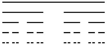
(a) Middle-$\mu$ Cantor set with $\mu=1/5$

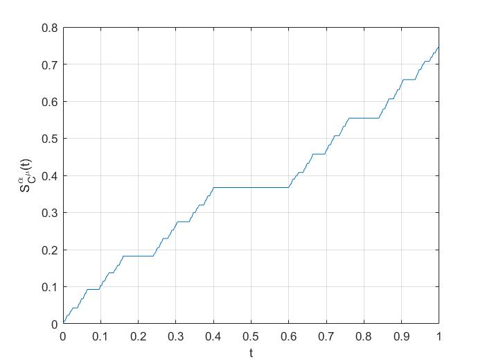
(b) Staircase function corresponding to middle-$\mu$ Cantor set with $\mu=1/5$

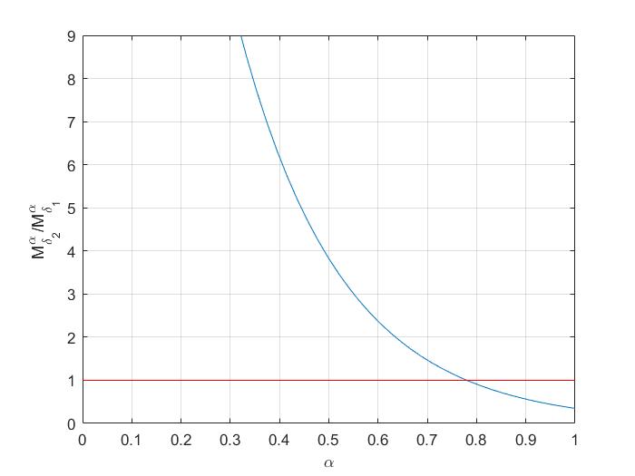
(c) The $\gamma$-dimension gives $\alpha=0.75$ to middle-$\mu$ Cantor set with $\mu=1/5$

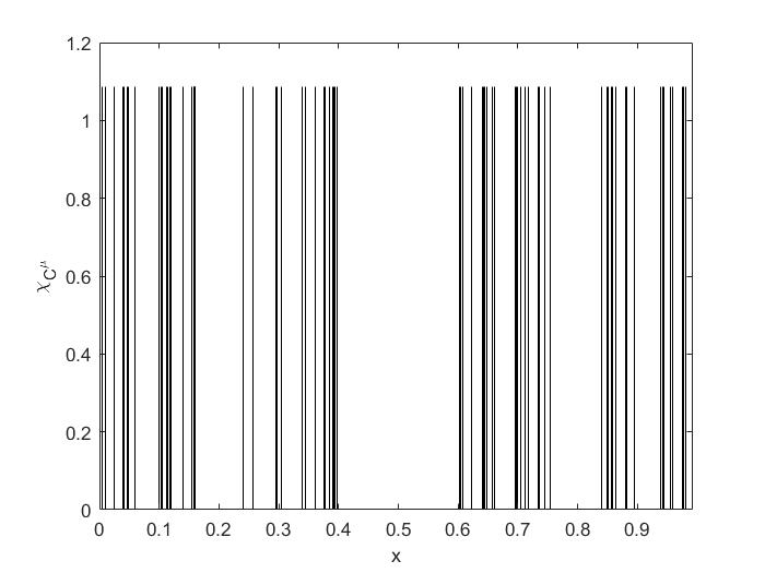
(d) Characteristic function for middle-$\mu$ Cantor set with $\mu=1/5$

Figure 1: Graphs corresponding to middle-$\mu$ Cantor set with $\mu=1/5$

The $C^{\mu}$-continuity of a function $h$ at $t\in C^{\mu}$ is defined in [25, 26] by

$$h(t)=\underset{z\rightarrow t}{\operatorname{C^{\mu}_{-}\lim}}~{}h(z).$$

The $C^{\mu}$-Differentiation of a function $h$ at $t\in C^{\mu}$ is defined in [25, 26, 28] by

$$D_{C^{\mu}}^{\alpha}h(t)=\begin{cases}\underset{z\rightarrow t}{\operatorname{C^{\mu}_{-}\lim}}\frac{h(z)-h(t)}{S_{C^{\mu}}^{\alpha}(z)-S_{C^{\mu}}^{\alpha}(t)},~{}~{}~{}\text{if }z\in C^{\mu},\\ 0,~{}~{}~{}~{}~{}~{}~{}~{}~{}~{}~{}~{}~{}~{}~{}~{}~{}~{}~{}~{}~{}~{}~{}~{}~{}~{}~{}~{}~{}~{}~{}\textmd{otherwise},\end{cases}$$

if limit exists.
The $C^{\mu}$-integral of $h$ on $[c_{1},c_{2}]$ is denoted by $\int_{c_{1}}^{c_{2}}h(t)d_{C^{\mu}}^{\alpha}t$ and is approximately given in [25, 26, 28] by

$$\int_{c_{1}}^{c_{2}}h(t)d_{C^{\mu}}^{\alpha}t\approx\sum_{i=1}^{m}h_{i}(t)(S_{C^{\mu}}^{\alpha}(t_{j})-S_{C^{\mu}}^{\alpha}(t_{j-1})).$$

We refer the reader for more meticulous definitions to see in [25, 26, 28]. In Figure 1 we have sketched the middle-$\mu$ Cantor, the staircase function, the characteristic function, and graph of $\mathcal{M}^{\alpha}_{\delta_{2}}/\mathcal{M}^{\alpha}_{\delta_{1}}$ versus to $\alpha$.

3 Fractal Lyapunov stability

In this section, we generalize the Lyapunov stability definition for the functions with fractal support.
Let us consider the following fractal differential equation with an initial condition

$$D_{K,t}^{\alpha}h(t)=g(h(t)),~{}~{}h(0)=h_{0},$$ (1)

where $g(h(t)):\Re\rightarrow\Re$, $C^{\mu}=K$ and $g$ has an equilibrium point $h_{e}$, then $g(h_{e})=0$.
1) The equilibrium point $h_{e}$ is called fractal Lyapunov stabile if we have

$$\forall~{}\epsilon>0,~{}\exists~{}\delta>0,~{}~{}~{}|h(0)-h_{e}|<\delta^{\alpha}\Rightarrow|h(t)-h_{e}|<\varepsilon^{\alpha},~{}~{}t\geq 0.$$

2) The stable equilibrium point $h_{e}$ is said fractal asymptotically stable if

$$\forall~{}\epsilon>0,~{}\exists~{}\delta>0,~{}~{}~{}|h(0)-h_{e}|<\delta^{\alpha}\Rightarrow\lim_{t\rightarrow\infty}|h(t)-h_{e}|=0.~{}~{}$$

3) The equilibrium point $h_{e}$ is called fractal exponentially stable if

$$~{}\exists~{}\delta>0,~{}~{}~{}|h(0)-h_{e}|<\delta^{\alpha}\Rightarrow|h(t)-h_{e}|\leq\kappa^{\alpha}|h(0)-h_{e}|e^{-\lambda\alpha t},~{}~{}$$

where $t\geq 0,~{}\kappa,\lambda\in\Re,$ and $~{}\kappa>0,~{}\lambda>0$.
Fractal Lyapunov function of Eq. (1) is a function $L:\Re\rightarrow\Re^{+},~{}R^{+}=[0,+\infty)$ which is $C^{\mu}$-continuous. Also, its $\alpha$-order derivative is $C^{\mu}$-continuous. Thus the fractal derivative of $L$ with respect to Eq.(1) is written as $L^{*}$ and if it has following condition

$$L^{*}=\frac{\partial L}{\partial h}g<0,\forall~{}t\in K~{}\backslash\{0\},$$ (2)

then, the zero solution of Eq. (1) is fractal asymptotically stable.
Example 1. Consider the following fractal differential equation

$$D_{K,t}^{\alpha}z(t)=-\chi_{K}z,~{}~{}~{}z(0)=c.$$ (3)

The general the solution of Eq. (3) is

$$z(t)=c\exp(-S_{K}^{\alpha}(t)).$$

A fractal Lyapunov function for studying the stability of Eq. (3) is

$$L(z)=z^{2}.$$ (4)

Then, we have

$$L^{*}=\frac{dL}{dz}(z)=-2z^{2}<0,~{}~{}(z\neq 0).$$ (5)

Thus, the zero solution of Eq.(3) is fractal asymptotically stable (See Figure 2(a)).

(a) Solution of Eq. (3) with $\mu=1/5$ and z(0)=1,0.5

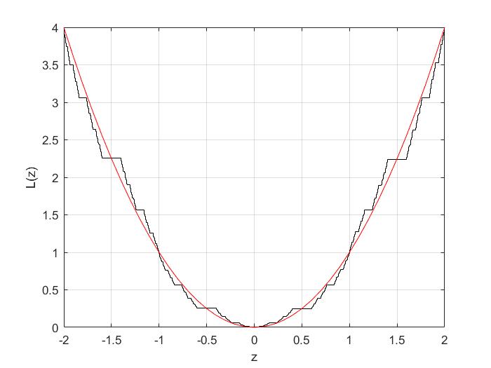
(b) Fractal Lyapunov function Eq. (3) with $\mu=1/5$

Figure 2: Graphs corresponding to Example 1.

In Figure 2 we have plotted the solution of Eq. (3) in 2(a) and corresponding Fractal Lyapunov function in 2(b).
Remark. In Figure 2, the red curves indicate the orbit of the solutions of Eq.(3) and Lyapunov function in the case of $\alpha=1$.

4 Qualitative behaviors of solutions of FDEs

In this section, we present the generalized conditions for the uniform boundedness and convergence of the solutions of the second $\alpha$-order of non-linear fractal differential equations. On the other hand, we modify and adopt the ordinary calculus conditions in fractal calculus [38]. The main results are obtained using the generalized Lyapunov function with the fractal sets support [25, 26, 28, 37, 38].
Let us consider the following second $\alpha$-order fractal differential equation

$$(D_{K,t}^{\alpha})^{2}y+u(S_{K}^{\alpha}(t))f(y,D_{K,t}^{\alpha}y)D_{K,t}^{\alpha}y+v(S_{K}^{\alpha}(t))h(y)=q(S_{K}^{\alpha}(t),y,z).~{}$$ (6)

By rewritten Eq. (6) in the form of the fractal system of differential equations and setting $S_{K}^{\alpha}(t)=t^{\prime}$, we obtain

$$D_{K,t}^{\alpha}y(t^{\prime}) = z(t^{\prime}),$$

$$D_{K,t}^{\alpha}z(t^{\prime}) = -u(t^{\prime})f(y,D_{K,t}^{\alpha}y)z(t^{\prime})-v(t^{\prime})h(y)$$ (7)

$$+ q(t^{\prime},y,z(t^{\prime})),$$

where $u(t^{\prime}),~{}v(t^{\prime}),~{}f(y,D_{K,t}^{\alpha}y),~{}h(y),~{}z(t^{\prime})=D_{K,t}^{\alpha}y$ and $q(t^{\prime},y,z)$ are $C^{\mu}$-continuous functions at every point $t\in C^{\mu}$ and they have well behavior such that the fractal uniqueness theorem holds for the fractal system (4). Meanwhile, $u(t^{\prime})$, $v(t^{\prime})$ are $C^{\mu}$-differentiable on $C^{\mu}$.
A. Assumptions

1. There are positive constants $u_{0},~{}v_{0},~{}E,~{}Q$, such that

   $$1\leq u_{0}^{\alpha} \leq u(t^{\prime})\leq E^{\alpha},$$

   $$1\leq v_{0}^{\alpha} \leq v(t^{\prime})\leq Q^{\alpha},$$

   where we consider $S_{K}^{\alpha}(t)<t^{\alpha}$ [25, 26, 28].

2. $\lambda_{1}(>0),~{}\lambda_{2}(>0)\in\Re$ and $\epsilon_{0},~{}\epsilon_{1},~{}\epsilon_{2}$ are small positive numbers such that

   $$\epsilon_{0}^{\alpha}\leq f(y,D_{K,t}^{\alpha}y).$$

3. $h(0)=0,~{}h(y)~{}\textmd{sgn}(y)>0,~{}(y\neq 0)$, such that

   $$H(y)=\int_{0}^{y}h(\lambda)d_{K}^{\alpha}\lambda\rightarrow\infty~{}\textmd{as}~{}|y|\rightarrow\infty,$$

   and

   $$0<\lambda_{2}\leq D_{K,t}^{\alpha}h(y).$$

4. $$\int_{0}^{\infty}\zeta_{0}(t^{\prime})d_{K}^{\alpha}t<\infty,~{}D_{K,t}^{\alpha}v(t^{\prime})\rightarrow 0~{}\textmd{as}~{}t\rightarrow\infty,$$

   where $\zeta_{0}(t^{\prime})=D_{K,t}^{\alpha}v_{+},~{}D_{K,t}^{\alpha}v_{+}=\max(D_{K,t}^{\alpha}v_{+},0)$.
   

Theorem 1. If assumptions (C1)-(C4) hold, then the zero solution of Eq.(6) when $q(S_{K}^{\alpha}(t),y,z)=0$ is fractal stable.
Proof: For proving this theorem we consider the following fractal Lyapunov function

$$L_{2}(t^{\prime},y,z)=\int_{0}^{y}h(\lambda)d_{K}^{\alpha}\lambda+\frac{z^{2}}{2v(t^{\prime})},$$ (8)

which is positive definite. By calculating fractal time derivative of (8) along the fractal system (4), we obtain

$$D_{K,t}^{\alpha}L_{2}=-\frac{D_{K,t}^{\alpha}v(t^{\prime})}{2v(t^{\prime})^{2}}z^{2}-\frac{u(t^{\prime})}{v(t^{\prime})}f(y,D_{K,t}^{\alpha}y)z^{2}.$$

We know that $v(t^{\prime})$ is an increasing function. Hence $D_{K,t}^{\alpha}v(t^{\prime})\geq 0$. Then, we have

$$D_{K,t}^{\alpha}L_{2}\leq-\frac{u(t^{\prime})}{v(t^{\prime})}f(y,D_{K,t}^{\alpha}y)z^{2}\leq 0.$$

In fact, it is obvious that $L_{2}(t^{\prime},0,0)=0$ and

$$L_{2}(t^{\prime},y,z) \geq \lambda_{2}y^{2}+\frac{z^{2}}{2v(t^{\prime})}$$

$$\geq \lambda_{2}y^{2}+\frac{z^{2}}{2Q^{\alpha}}$$

$$\geq \bar{\lambda}(y^{2}+z^{2}),$$

where $\bar{\lambda}=\min(\lambda_{2},\frac{1}{2Q^{\alpha}})$. Then the proof is complete.
B. Assumption

1. There are positive constants $0\leq\sigma\leq 1,~{}0\leq\Delta\leq 1$, such that

   $$\int_{0}^{\infty}r_{i}(t^{\prime})d_{K}^{\alpha}t,~{}~{}~{}r_{1}(t^{\prime}),~{}r_{2}(t^{\prime})>0,~{}~{}~{}(i=1,2),$$

   are $C^{\mu}$-Continuous functions and

   $$|q(t^{\prime},y,z(t^{\prime}))|\leq r_{1}(t^{\prime})+r_{2}(t^{\prime})[H(y)+z^{2}]^{\sigma^{\prime}/2}+\Delta^{\alpha}|z|,$$

   where $\sigma^{\prime}=\sigma^{\alpha}$.

2. $$\epsilon_{0}^{\alpha}\leq f(y,D_{K,t}^{\alpha}y)-\lambda_{1}\leq\epsilon_{1}^{\alpha}.$$

3. $$0\leq\lambda_{2}-D_{K,t}^{\alpha}h(y)\leq\epsilon_{2}^{\alpha}.$$

Theorem 2. Let $q(S_{K}^{\alpha}(t),y,z)\neq 0$ and assume $(C1)-(C5)$ hold. Then the solutions of Eq.(6) are fractal uniformly bounded and fractal convergent, namely

$$y(t^{\prime})\rightarrow 0,~{}D_{K,t}^{\alpha}y(t^{\prime})\rightarrow 0,~{}\textmd{as}~{}S_{K}^{\alpha}(t)\rightarrow 0.$$ (9)

To prove this theorem, we define a fractal Lyapunov function for Eq.(6) by

$$L_{0}(t^{\prime},y,z)=v(t^{\prime})\int_{0}^{y}h(\lambda)d_{K}^{\alpha}\lambda+\frac{z^{2}}{2}+k,$$ (10)

where $k$ is positive constant.
Before giving the proof of the above theorem, we present two lemmas, Lemma 1 and Lemma 2, which are needed in the proof of the theorem.
Lemma 1. If assumptions (C1) and (C3) hold, then

$$E_{1}^{1/\alpha}[H(y)+z^{2}+k]\leq L_{0}(t^{\prime},y,z)\leq E_{2}^{1/\alpha}[H(y)+z^{2}+k],~{}~{}\exists~{}E_{1}>0,~{}E_{2}>0\in\Re.$$

Proof: In view of assumptions (C1) and (C3) we can derive

$$L_{0}\geq v_{0}^{\alpha}\int_{0}^{y}h(\lambda)d_{K}^{\alpha}\lambda+\frac{z^{2}}{2}+k\geq E_{1}^{\alpha}[H(y)+z^{2}+k],$$

where $E_{1}=\min(v_{0},1/2)$.
In the same manner, by assumptions (C1) and (C3), we can obtain

$$L_{0}\leq Q^{\alpha}\int_{0}^{y}h(\lambda)d_{K}^{\alpha}\lambda+\frac{z^{2}}{2}+k\leq E_{2}^{\alpha}[H(y)+z^{2}+k],$$

where $E_{2}=\max(Q,1)$. $\Box$
Lemma 2. If assumptions (C1)-(C4) are valid, then

$$\exists~{}E_{3}>0,~{}E_{4}>0,~{}D_{K,t}^{\alpha}L_{0}\leq-E_{3}^{\alpha}z^{2}+(r_{1}(t^{\prime})+r_{2}(t^{\prime}))|z|+r_{2}(t^{\prime})[H(y)+z^{2}]+E_{4}^{\alpha}\zeta_{0}L_{0},$$

where $E_{3},E_{4}\in\Re$.
Proof: Fractal differentiating of the fractal Lyapunov function (10) along with fractal system (4), we get

$$D_{K,t}^{\alpha}L_{0}=-u(t^{\prime})f(y,z)z^{2}+q(t^{\prime},y,z)z+D_{K,t}^{\alpha}v(t^{\prime})\int_{0}^{y}h(\lambda)d_{K}^{\alpha}\lambda.$$

By using the assumptions of the Theorem 2, we obtain

$$D_{K,t}^{\alpha}L_{0} \leq -E^{\alpha}(\lambda_{1}+\epsilon_{0})z^{2}+|q(t^{\prime},y,z)||z|+\zeta_{0}H(y)$$

$$\leq -2E_{3}^{\alpha}z^{2}+|q(t^{\prime},y,z)||z|+E_{4}^{\alpha}\zeta_{0}L_{0},$$

where

$$E_{3}=E(\lambda_{1}+\epsilon_{0})/2,~{}E_{4}=(1/E_{1}).$$

Here, in view of (C5), the term $|q(t^{\prime},y,z)||z|$ can be written as

$$|q(t^{\prime},y,z)||z|\leq\bigg{(}r_{1}(t^{\prime})+r_{2}(t^{\prime})[H(x)+z^{2}]^{\sigma^{\prime}/2}\bigg{)}|z|+\Delta^{\alpha}z^{2}.$$

Hence, we have

$$D_{K,t}^{\alpha}L_{0}\leq-2E_{3}^{\alpha}z^{2}+(r_{1}(t^{\prime})+r_{2}(t^{\prime})[H(x)+z^{2}]^{\sigma^{\prime}/2})|z|+\Delta^{\alpha}z^{2}+E_{4}^{\alpha}\zeta_{0}L_{0}.$$

Set $\Delta=E_{3}$. Then

$$D_{K,t}^{\alpha}L_{0}\leq-E_{3}^{\alpha}z^{2}+(r_{1}(t^{\prime})+r_{2}(t^{\prime})[H(x)+z^{2}]^{\sigma^{\prime}/2})|z|+E_{4}^{\alpha}\zeta_{0}L_{0}.$$ (11)

Using the following inequality

$$[H(x)+z^{2}]^{\sigma^{\prime}/2}\leq 1+[H(x)+z^{2}]^{1/2},$$ (12)

taking into account (11) and (12) we obtain

$$D_{K,t}^{\alpha}L_{0}\leq-E_{3}^{\alpha}z^{2}+(r_{1}(t^{\prime})+r_{2}(t^{\prime}))|z|+r_{2}(t^{\prime})[H(x)+z^{2}]+E_{4}^{\alpha}\zeta_{0}L_{0}.~{}$$

To complete the proof of the theorem, we consider the fractal Lyapunov function $L_{0}$ defined by

$$L(t^{\prime},y,z)=e^{-\int_{0}^{t}\zeta(\theta)d_{K}^{\alpha}\theta}L_{0}(t^{\prime},y,z),$$ (13)

where

$$\zeta(t^{\prime})=E_{4}^{\alpha}\zeta_{0}+\frac{4}{E_{1}^{\alpha}}(r_{1}(t^{\prime})+r_{2}(t^{\prime})),$$

and

$$\psi_{1}(||\bar{y}||)\leq V(t^{\prime},y,z)\leq\psi_{2}(||\bar{y}||),$$ (14)

with $\bar{y}=(y,z)\in\Re^{2}$ and $t\in C^{\mu}$, and $\psi_{1},\psi_{2}$ are $C^{\mu}$-continuous and increasing functions such that $\psi_{1}(||\bar{y}||)\rightarrow\infty$ while $||\bar{y}||\rightarrow\infty$.
Fractal differentiating fractal Lyapunov function (13) and considering the fractal system (4) and assumptions of Theorem 2, we have

$$D_{K,t}^{\alpha}L(t^{\prime},y,z) =e^{-\int_{0}^{t}\zeta(\theta)d_{C^{\mu}}^{\alpha}\theta}[D_{K,t}^{\alpha}L_{0}-\zeta(t^{\prime})L_{0}]$$

$$\leq e^{-\int_{0}^{t}\zeta(\theta)d_{K}^{\alpha}\theta}[-E_{3}^{\alpha}z^{2}+(r_{1}(t^{\prime})+r_{2}(t^{\prime}))|z|+r_{2}(t^{\prime})[H(y)+z^{2}]$$

$$-4(r_{1}(t^{\prime})+r_{2}(t^{\prime}))(H(y)+z^{2}+k)]$$

$$\leq e^{-\int_{0}^{t}\zeta(\theta)d_{K}^{\alpha}\theta}[-E_{3}^{\alpha}z^{2}+(r_{1}(t^{\prime})+r_{2}(t^{\prime}))|z|$$

$$-2(r_{1}(t^{\prime})+r_{2}(t^{\prime}))(H(y)+z^{2}+k)]$$

$$\leq e^{-\int_{0}^{t}\zeta(\theta)d_{K}^{\alpha}\theta}[-E_{3}^{\alpha}z^{2}-2(r_{1}(t^{\prime})+r_{2}(t^{\prime}))\{(|z|-\frac{1}{4})^{2}-\frac{1}{16}+2k\}].$$

If we choose $k\geq\frac{1}{32}$, then it follows that there exists a positive $E_{5}$ such that

$$D_{K,t}^{\alpha}L(t^{\prime},y,z)\leq-E_{5}^{\alpha}z^{2}.$$ (15)

By considering (14) and (15) it follows that all solutions of Eq.(4) are fractal uniformly bounded.
Consider the fractal system of differential equations

$$D_{K,t}^{\alpha}\bar{y}=M(t^{\prime},\bar{y})+N(t^{\prime},\bar{y}),$$ (16)

where $M,N$ are $C^{\mu}\subset\Re^{+}$-continuous and vector functions, and $C^{\mu}\times Q\subset\Re^{2}$ is an open set. Moreover, it is clear that

$$||N(t^{\prime},\bar{y})||\leq N_{1}(t^{\prime},\bar{y})+N_{2}(\bar{y}),$$

where $N_{1}(t^{\prime},\bar{y}),N_{2}(\bar{y})$ are $C^{\mu}$-continuous and non-negative functions. $\Box$
Lemma 3. Let $L:C^{\mu}\times Q$ be a function $C^{\mu}$-continuous and $C^{\mu}$-differentiable such that

$$D_{K,t}^{\alpha}L(t^{\prime},\bar{y})\leq-B(||\bar{y}||),$$

where $B(||\bar{y}||)$ is a positive definite in the closed set $\Psi\in Q$ and $M(t^{\prime},\bar{y})$ satisfies the following.

1. $M(t^{\prime},\bar{y})$ tends to $K(\bar{y})$ for $\bar{y}\in\Psi$ as $t\rightarrow\infty$, $K(\bar{y})$ is a $C^{\alpha}$-continuous on $\Psi$.

2. $$\forall~{}\epsilon>0,~{}\bar{y}\in\Psi,~{}\exists~{}\delta=\delta(\epsilon,\bar{z})>0,~{}T=T(\epsilon,~{}\bar{z})>0,$$

   such that if

   $$t\geq T,~{}||\bar{y}-\bar{z}||<\delta(\epsilon,\bar{z}),$$

   we have

   $$||M(t^{\prime},\bar{y})-M(t^{\prime}-\bar{z})||<\epsilon^{\alpha}.$$

3. $N_{2}(\bar{y})$ is positive definite on closed $\Psi$ of $Q$.

Then every bounded solution of Eq.(16) approaches to the fractal system

$$D_{K,t}^{\alpha}\bar{y}=\mathfrak{K}(\bar{y}),$$ (17)

which is contained in $\Psi$ as $t\rightarrow\infty.$
Proof. Now, we consider (4). It follows that

$$M(t^{\prime},\bar{y})=\left(\begin{array}[]{c}z\\ -u(t^{\prime})f(y,z)z-v(t^{\prime})h(y)\\ \end{array}\right)$$

and

$$N(t^{\prime},\bar{y})=\left(\begin{array}[]{c}0\\ q(t^{\prime},y,z)\\ \end{array}\right).$$

Then

$$||N(t^{\prime},\bar{y})||\leq(r_{1}(t^{\prime})+r_{2}(t^{\prime}))[H(y)+z^{2}]^{\sigma^{\prime}/2}+\Delta^{\alpha}|z|.$$

We can also write

$$N_{1}(t^{\prime},\bar{y})=r_{1}(t^{\prime})+r_{2}(t^{\prime})[H(y)+z^{2}]^{\sigma^{\prime}/2}$$

and

$$N_{2}(\bar{y})=\Delta^{\alpha}|z|.$$

The functions $M(t^{\prime},\bar{y})$ and $N(t^{\prime},\bar{y})$ satisfy the conditions of Lemma 3. Set $\psi_{1}(||\bar{y}||)=E_{5}^{\alpha}z^{2}$, then

$$D_{F,t}^{\alpha}L(t^{\prime},y,z)\leq-\psi_{1}(||\bar{y}||),$$

where the function $||\bar{y}||$ is positive definite on $\Psi=\{(y,z)|y\in\Re,z=0\}$. We get

$$M(t^{\prime},\bar{y})=\left(\begin{array}[]{c}0\\ -v(t^{\prime})h(y)\\ \end{array}\right)$$

by using (C4) condition of Theorem 1. If we suppose

$$\mathfrak{K}(\bar{y})=\left(\begin{array}[]{c}0\\ -v_{\infty}h(y)\\ \end{array}\right),$$ (18)

then all the conditions of Lemma 3 are satisfied. It is straight forward to see that $N_{2}(\bar{y})$ is positive definite function. Since the solutions of fractal system (4) are bounded, therefore by using Lemma 3 we have

$$D_{K,t}^{\alpha}\bar{y}=\mathfrak{K}(\bar{y}),$$

which is semi-invariant set of the fractal system contained in $\Psi$ as $t\rightarrow\infty$. In view of (18), we have following

$$D_{K,t}^{\alpha}y=0,~{}~{}~{}D_{K,t}^{\alpha}z=-v_{\infty}h(y).$$ (19)

Fractal system Eq.(19) has solution

$$y=c_{1},~{}~{}~{}z=c_{2}-v_{\infty}h(c_{1})(S_{K}^{\alpha}(t)-S_{K}^{\alpha}(t_{0})).$$

In order to remain in $\Psi$, the solutions must be

$$c_{2}-v_{\infty}h(c_{1})(S_{K}^{\alpha}(t)-S_{K}^{\alpha}(t_{0}))=0,\forall~{}t\geq t_{0},$$

which implies $k=0,h(c_{1})=0$, so that $c_{1}=c_{2}=0$. Then $\bar{y}=\bar{0}$ is the solution of $D_{K,t}^{\alpha}\bar{y}=\mathfrak{K}(\bar{y})$ remaining in $\Psi$. Consequently, we arrive at

$$y(t^{\prime})\rightarrow 0,~{}~{}~{}D_{K,t}^{\alpha}y(t^{\prime})\rightarrow 0,~{}as~{}t\rightarrow 0.~{}\Box$$

Example 2. Consider the fractal differential equation

$$(D_{K,t}^{\alpha})^{2}y(t)+s(y)D_{K,t}^{\alpha}y(t)+h(y)=0.$$ (20)

This is equivalent to the fractal system

$$D_{K,t}^{\alpha}y = z-S(y)$$

$$D_{K,t}^{\alpha}z = -h(y),$$ (21)

where

$$S(y)=\int_{0}^{y}s(\beta)d_{K}^{\alpha}\beta.$$

and, if we suppose

$$H(y)=\int_{0}^{y}h(\rho)d_{K}^{\alpha}\rho,$$

Consider the fractal function

$$L_{1}(y,z)=H(y)+\frac{z^{2}}{2},$$ (22)

which is a strong fractal Lyapunov function. Fractal differentiating of $L_{1}(y,z)$ and Eq.(22) we get

$$D_{K,t}^{\alpha}L_{1}(y,z)=h(y)D_{K,t}^{\alpha}y+zD_{K,t}^{\alpha}z=-h(y)S(y).$$

Using the assumption theorem we obtain

$$D_{K,t}^{\alpha}L_{1}(y,z)=-h(y)S(y)<0,$$

which shows that the solutions of Eq.(20) are fractal uniformly bounded and fractal ultimately bounded.
Example 3. Consider harmonic oscillator on the fractal time as follows:

$$(D_{K,t}^{\alpha})^{2}y(t)+\mathfrak{C}_{K}y(t)=0,~{}t\in K,~{}\mathfrak{C}_{K}>0,$$ (23)

where $\mathfrak{C}_{K}$ is constant. The equivalent fractal system is

$$D_{K,t}^{\alpha}y = z,$$

$$D_{K,t}^{\alpha}z = -\mathfrak{C}_{K}y.$$ (24)

The fractal Lyapunov function correspond to Eq.(23) is

$$L(y,z)=\frac{1}{2}\mathfrak{C}_{K}y^{2}+\frac{1}{2}z^{2},$$ (25)

where $L(0,0)=0$ and $L(y,z)>0$ for $(y,z)\in\Re^{2}\backslash(0,0)$.

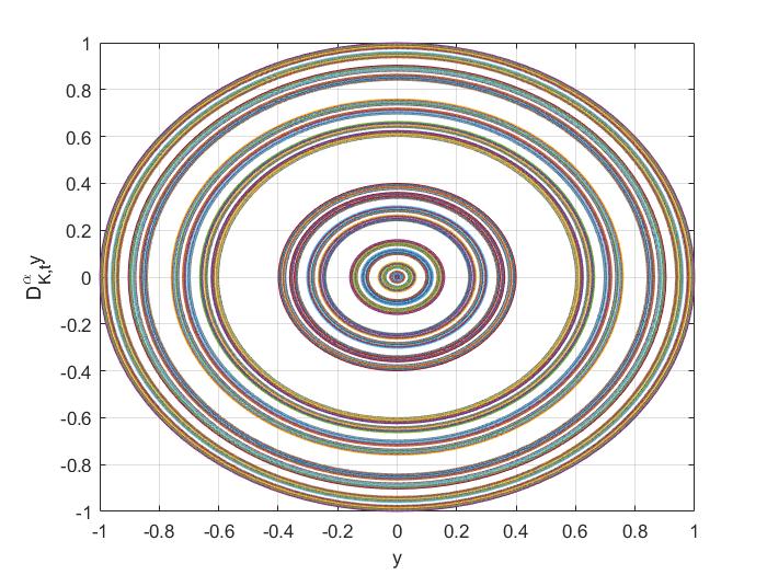
(a) Solution of Eq. (23) with $\mu=1/5$ and

(b) Fractal Lyapunov function Eq. (23) with $\mu=1/5$

Figure 3: Graphs corresponding to Example 2.

Then, it is obtain that

$$D_{K,t}^{\alpha}L(y,z)=\frac{\partial}{\partial y}L(y,z)D_{K,t}^{\alpha}y+\frac{\partial}{\partial y},L(y,z)D_{K,t}^{\alpha}z=0.$$

Hence, the zero solution $(0,0)$ is a fractal stable point. In Figure 3, we have sketched solutions of Eq. (23) and Eq. (25).

5 Conclusion

In this paper, we have suggested conditions for the fractal stability, uniformly boundedness and the asymptotic behaviors of solutions of second $\alpha$-order fractal differential equations. The analogous theorems of stability, uniformly boundedness and asymptotic behavior to standard calculus have been given and adopted in fractal calculus. The generalized conditions include solutions and functions which are non-differentiable in sense of ordinary calculus.

Acknowledgement:
This research was completed with the support of the Scientific and Technological Research Council of Turkey (TÜBİTAK) (2221-Fellowships for Visiting Scientists and Scientists on Sabbatical Leave – 2221-2018/3 period) when Alireza Khalili Golmankhaneh was a visiting scholar at Van Yuzunçu Yil University, Van, Turkey

References

- [1] B.B. Mandelbrot, The fractal geometry of nature. Vol (173) New York: WH freeman, 1983.
- [2] M.F. Barnsley, Fractals Everywhere, Academic press, 2014.
- [3] C. Cattani, fractals and hidden symmetries in DNA, Math. Probl. Eng., vol. 2010, Article ID 507056, 31 pages, 2010. https://doi.org/10.1155/2010/507056.
- [4] M. S. Tavazoei, M. Haeri, An optimization algorithm based on chaotic behavior and fractal nature, J. Comput. Appl. Math, 206(2) (2007) 1070-1081.
- [5] E. Nakaguchi, M. Efendiev, On a new dimension estimate of the global attractor for chemotaxis-growth systems, Osaka J. Math., 45(2) (2008), 273-281.
- [6] M. Efendiev, S. Zelik, Finite- and infinite-dimensional attractors for porous media equations, Proc. Math. Phys. Eng. Sci., 96(1) (2008), 51-77.
- [7] I. Chitescu, H. Georgescu, R.Miculescu, Approximation of infinite dimensional fractals generated by integral equations, J. Comput. Appl. Math, 234(5) (2010), 1417-1425.
- [8] S. Ree, L. Reichl, Fractal analysis of chaotic classical scattering in a cut-circle billiard with two openings, Phys. Rev. E 65(5) (2002), 055205.
- [9] E.de Amo I.Chitescu, M.Díaz Carrillo, N.A. Secelean, A new approximation procedure for fractals, J. Comput. Appl. Math, 151(2) (2003), 355-370.
- [10] L. Nottale, J. Schneider, Fractals and nonstandard analysis, J. Math. Phys., 25(5) (1998), 1296-1300.
- [11] M.N. Célérier, L. Nottale, Quantum-classical transition in scale relativity, J. Phys. A: Math. Gen, 37 (2004), 931–955.
- [12] K. Falconer, Fractal geometry: mathematical foundations and applications. John Wiley Sons, 2004.
- [13] K. Falconer, Techniques in fractal geometry. Wiley (1997).
- [14] G. Edgar, Measure, topology, and fractal geometry. Springer Science Business Media, 2007.
- [15] J. Kigami, Analysis on Fractals, Cambridge University Press, 2001.
- [16] F.H. Stillinger, Axiomatic basis for spaces with noninteger dimension. J. Math. Phys., 18(6) (1977), 1224-1234.
- [17] V.E. Tarasov, Fractional dynamics: applications of fractional calculus to dynamics of particles, fields and media. Springer Science Business Media, 2011.
- [18] M. Zubair, M.J. Mughal, Q.A. Naqvi, Electromagnetic Fields and Waves in Fractional Dimensional Space, Springer, New York, 2012.
- [19] W. Chen Y. Liang, New methodologies in fractional and fractal derivatives modeling. Chaos, Soliton Fract., 102 (2017), 72-77.
- [20] Y. Liang, A. Q. Ye, W. Chen, R. G. Gatto, L. Colon-Perez, T. H. Mareci, R. L. Magin, A fractal derivative model for the characterization of anomalous diffusion in magnetic resonance imaging, Commun. Nonlinear Sci. Numer. Simul., 39 (2016), 529-537.
- [21] R. Herrmann, Fractional calculus: an introduction for physicists, World Scientific, 2014.
- [22] S. Das, Functional fractional calculus, Springer Science Business Media, 2011.
- [23] K.M. Kolwankar, A.D. Gangal, Fractional differentiability of nowhere differentiable functions and dimensions, Chaos, 6(4) (1996), 505-513.
- [24] K.M. Kolwankar, A.D. Gangal, Local Fractional Fokker-Planck Equation, Phys. Rev. Lett. 80 (1998), 214.
- [25] A. Parvate, A.D. Gangal, Calculus on fractal subsets of real-line I: Formulation, Fractals, 17(01) (2009), 53-148.
- [26] A. Parvate, A.D. Gangal, Calculus on fractal subsets of real line II: Conjugacy with ordinary calculus, Fractals, 19(03) (2011), 271-290.
- [27] A. Parvate, S. Satin , A.D. Gangal, Calculus on fractal curves in , Fractals, 19(1) (2011), 15–27.
- [28] A.K. Golmankhaneh, A. Fernandez, A.K. Golmankhaneh, D. Baleanu, Diffusion on middle- Cantor sets, Entropy, 20(504) (2018), 1-13.
- [29] A.K. Golmankhaneh, A.S. Balankin, Sub-and super-diffusion on Cantor sets: Beyond the paradox, Phys. Lett. A, 382(14) (2018), 960-967.
- [30] A.K. Golmankhaneh, Quantum mechanics on the fractal time-space, In Proceedings of the 8th International Conference on Fractional Differentiation and its Applications,2016, July, Novi Sad, Serbia.
- [31] A.K. Golmankhaneh, C. Tunç, Sumudu transform in fractal calculus, Appl. Math. Comput., 350 (2019), 386-401.
- [32] A.K. Golmankhaneh, C. Tunç, On the Lipschitz condition in the fractal calculus, Chaos, Soliton Fract., 95 (2017), 140-147.
- [33] G.C. Wu, D. Baleanu, W.H. Luo, Lyapunov functions for Riemann-Liouville-like fractional difference equations, Appl. Math. Comput., 314 (2017), 228-236.
- [34] M. Rivero, S. V. Rogosin, J. A. T. Machado, J. J. Trujillo, Stability of fractional order systems, Math. Probl. Eng., vol. 2013, Article ID 356215, 14 pages, 2013. https://doi.org/10.1155/2013/356215.
- [35] R. Agarwal, S. Hristova, D. O’Regan, A survey of Lyapunov functions, stability and impulsive Caputo fractional differential equations, Fract. Calc. Appl. Anal., 19(2) (2016), 290-318.
- [36] A.Q.M. Khaliq, X. Liang, K.M. Furati, A fourth-order implicit-explicit scheme for the space fractional nonlinear Schrödinger equations, Numer. Algorithms, 75(1) (2016), 147–172
- [37] C. Tunç, Uniformly stability and boundedness of solutions of second order nonlinear delay differential equations, Appl. Comput. Math. 10(3) (2011), 449–462.
- [38] C. Tunç, E. Tunç, On the asymptotic behavior of solutions of certain second-order differential equations, J. Franklin Inst. 344(5) (2007), 391–398.
- [39] T. Yoshizawa, Stability theory by Liapunov’s second method. Publications of the Mathematical Society of Japan, vol. 9, The Mathematical Society of Japan, Tokyo, 1966.
- [40] T. Hara, On the asymptotic behavior of the solutions of some third and fourth order non-autonomous differential equations, Pub. Res. I. Math. Sci, 9(3) (1974), 649-673.
- [41] R. DiMartino, W. Urbina, On Cantor-like sets and Cantor-Lebesgue singular functions,arXiv preprint arXiv:1403.6554 (2014).