Recent probes of standard and non-standard neutrino physics with nuclei

Abstract

We review standard and non-standard neutrino physics probes that are based on nuclear measurements. We pay special attention on the discussion of prospects to extract new physics at prominent rare event measurements looking for neutrino-nucleus scattering, such as the coherent elastic neutrino-nucleus scattering (CE$\nu$NS) that may involve lepton flavor violation (LFV) in neutral-currents (NC). For the latter processes several appreciably sensitive experiments are currently pursued or have been planed to operate in the near future, like the COHERENT, CONUS, CONNIE, MINER, TEXONO, RED100, vGEN, Ricochet, NUCLEUS etc. We provide a thorough discussion on phenomenological and theoretical studies, in particular those referring to the nuclear physics aspects in order to provide accurate predictions for the relevant experiments. Motivated by the recent discovery of CE$\nu$NS at the COHERENT experiment and the active experimental efforts for a new measurement at reactor-based experiments, we summarize the current status of the constraints as well as the future sensitivities on nuclear and electroweak physics parameters, non-standard interactions, electromagnetic neutrino properties, sterile neutrinos and simplified scenarios with novel vector $Z^{\prime}$ or scalar $\phi$ mediators. Indirect and direct connections of CE$\nu$NS with astrophysics, direct Dark Matter detection and charge lepton flavor violating processes are also discussed.

I Introduction

During the last few decades, intense research effort has been devoted to multidisciplinary neutrino searches involving physics within and beyond the standard model (SM) in the theory, phenomenology and experiments that drops in the interplay of particle, nuclear physics, astrophysics and cosmology.

Astrophysical and laboratory searches [1] offer unique opportunities to probe great challenges in modern-day physics such as the underlying physics of the fundamental electroweak interactions within and beyond the SM [2, 3] in the neutral and charged-current sector of semi-leptonic neutrino-nucleus processes [4, 5, 6]. To meet the sufficient energy and flux requirements, the relevant studies consider different low-energy neutrino sources including (i) Supernova (SN) neutrinos, (ii) accelerator neutrinos (from pion decay at rest, $\pi$-DAR) and (iii) reactor neutrinos, while interesting proposals aiming to use ⁵¹Cr and beta-beam neutrino sources have appeared recently. The detection mechanism of low-energy neutrino interactions with nucleons and nuclei is experimentally hard and limited by the tiny nuclear recoils produced by the scattering process. To this purpose, the nuclear detector materials are carefully selected to fulfill the requirement of achieving a-few-keV or sub-keV threshold capabilities. The detectors developed are based on cutting edge technologies such as scintillating crystals (CsI[Na], NaI[Tl]), p-type point-contact (PPC) germanium detectors, single-phase or double liquid noble gases (LAr, LXe) charged coupled devices (CCDs), cryogenic bolometers, etc.

The neutral-current coherent elastic neutrino nucleus scattering (CE$\nu$NS) was proposed about four decades ago [7, 8, 9], while it was experimentally confirmed in 2017 by the COHERENT Collaboration [10] at the Spallation Neutron Source, in good agreement with the SM expectation. The observation of CE$\nu$NS has opened up a new era, triggering numerous theoretical studies to interpret the available data [11] in a wide spectrum of new physics opportunities, with phenomenological impact on astroparticle physics, neutrino oscillations, dark matter (DM) detection, etc. (see Ref. [12] for various applications). In particular, the recent works have concentrated on non-standard interactions (NSI) [13, 14, 15, 16, 17, 18, 19], electromagnetic properties [20, 21, 22, 23], sterile neutrinos [24, 25, 26], CP-violation [27] and novel mediators [28, 29, 30, 31]. Nuclear and atomic effects are explored in Refs. [32, 33, 34, 35, 36, 37, 38] which may have direct implications to the neutrino-floor [39, 40, 41] and to DM searches [42, 43, 44]. Being a rapidly developing field, there are several experimental programs aiming to observe CE$\nu$NS in the near future, such as the TEXONO [45], CONNIE [46], MINER [47], vGEN [48], CONUS [49], Ricochet [50] and NUCLEUS [51].

Future CE$\nu$NS measurements have good prospects to shed light on the exotic neutrino-nucleus interactions expected in the context of models describing flavor changing neutral-current (FCNC) processes [52] as well as to subleading NSI oscillation effects [53, 54, 55, 56, 57] and various open issues in nuclear astrophysics [58, 59]. The main goal of this review article is to provide an up-to-date status of the conventional and exotic neutrino physics probes of CE$\nu$NS and to summarize the necessary aspects for the interpretation of the experimental data. We focus on the theoretical modelling, calculations and analysis of the data that are relevant at the time of writing and we mainly concentrate on the theoretical and phenomenological physics aspects. For a recent review on the experimental advances of CE$\nu$NS, see Ref. [60].

This review article has been organized as follows: Sect. II provides the theoretical treatment of low-energy neutrino-nucleus processes for both coherent and incoherent channels and its connection to the more general lepton-nucleus case with a particular emphasis on the nuclear physics aspects. Sect. III presents the current status of constraints on SM and exotic physics parameters resulted from the analysis of the COHERENT data and discusses the projected sensitivities from future CE$\nu$NS measurements at $\pi$-DAR and reactor facilities. In Sect. IV we briefly summarize the most important connections of CE$\nu$NS with DM searches, charged lepton flavor violation (cLFV) and astrophysics. Finally, the main conclusions are given in Sect. V.

II Theoretical study of neutrino-nucleus interaction

At low- and intermediate-energies, the neutrino being a key input to understand open issues in physics within and beyond the SM (see below), necessitated a generation of neutrino experiments for exploring neutrino scattering processes with nucleons and nuclei for both charged-current (inelastic) and neutral-current (coherent elastic and incoherent scattering) processes. Theoretically, the neutral-current neutrino-nucleus scattering we are interested here, is a well studied process for both coherent [61] an incoherent channels [62, 63]. The accurate evaluation of the required transition matrix elements describing the various interaction channels of the electroweak processes between an initial and a final (many-body) nuclear state, is obtained on the basis of reliable nuclear wavefunctions. From a nuclear theory point of view, such results have been obtained by paying special attention on the accurate contruction of the nuclear ground state in the framework of the quasi-particle random phase approximation (QRPA), using schematic Skyrme [64] or realistic Bonn C-D pairing interactions [65]. Focusing on the latter method, the authors of Ref. [61] solved iteratively the Bardeen-Cooper-Schrieffer (BCS) equations, achieving a high reproducibility of the available nuclear charge-density-distribution experimental data [66].

II.1 Coherent and incoherent neutrino-nucleus cross sections

In the Donnelly-Walecka theory [67] all semi-leptonic nuclear processes at low and intermediate energies may be described by an effective interaction Hamiltonian through the leptonic $j_{\mu}^{\text{lept}}$ and hadronic $\mathcal{J}_{\mu}$ current densities,

$$\hat{H}_{eff}=\frac{G}{\sqrt{2}}\int\hat{\ell}_{\mu}^{\mathrm{lept}}({\bf x})\hat{\mathcal{J}}^{\mu}({\bf x})\,d^{3}{\bf x}\,,$$ (1)

where $G=G_{F}$ is the Fermi coupling constant for neutral-current processes and $G=G_{F}\rm{cos}\theta_{c}$ ($\theta_{c}$ is the Cabbibo angle) for charged-current processes. For partial scattering rates, the evaluation of the transition amplitudes $\langle f|\hat{H}_{eff}|i\rangle$ are treated via a multipole decomposition analysis of the hadronic current (see the Appendix A.1). Then, for a given set of an initial $|J_{i}\rangle$ and a final $|J_{f}\rangle$ nuclear state, the double differential SM cross section becomes [68]

$$\frac{d^{2}\sigma_{i\rightarrow f}}{d\Omega\,d\omega}=\frac{G^{2}}{\pi}F(Z,\varepsilon_{f})\frac{|\mathbf{k}_{f}|\varepsilon_{f}}{(2J_{i}+1)}\left(\sum_{J=0}^{\infty}\sigma_{\mathrm{CL}}^{J}+\sum_{J=1}^{\infty}\sigma_{\mathrm{T}}^{J}\right),$$ (2)

with $\varepsilon_{f}$ ($|\mathbf{k}_{f}|$) denoting the final energy (momentum) of the outgoing lepton, while $\omega=\varepsilon_{i}-\varepsilon_{f}$ stands for the excitation energy of the nucleus where $\varepsilon_{i}$ is the initial lepton energy. For charged-current processes, the Fermi function $F(Z,\varepsilon_{f})$, takes into account the final state interaction of the outgoing charged particle, while for neutral-current processes such as coherent and incoherent neutrino-nucleus scattering it is $F(Z,\varepsilon_{f})=1$.

The individual cross sections in Eq.(2) receive contributions from the so-called Coulomb $\hat{\mathcal{M}}$, longitudinal $\hat{\mathcal{L}}$, transverse electric $\hat{\mathcal{T}^{el}}$ and transverse magnetic $\hat{\mathcal{T}^{mag}}$ operators for both vector and axial vector components (see the Appendix A.1). The cross sections $\sigma_{\mathrm{CL}}^{J}$ and $\sigma_{\mathrm{T}}^{J}$ are expressed in terms of the reduced matrix elements of the eight basic irreducible tensor operators [67]

$$\sigma_{\mathrm{CL}}^{J}= (1+a\rm{cos}\theta)|\langle J_{f}||\hat{\mathcal{M}}_{J}(\kappa)||J_{i}\rangle|^{2}$$ (3)

$$+(1+a\rm{cos}\theta-2b\rm{sin}^{2}\theta)|\langle J_{f}||\hat{\mathcal{L}}_{J}(\kappa)||J_{i}\rangle|^{2}$$

$$+\left[\frac{\omega}{\kappa}(1+a\rm{cos}\theta)+d\right]2\Re e|\langle J_{f}||\hat{\mathcal{L}}_{J}(\kappa)||J_{i}\rangle||\langle J_{f}||\hat{\mathcal{M}}_{J}(\kappa)||J_{i}\rangle|^{\ast}\,,$$

$$\sigma_{\mathrm{T}}^{J}= (1-a\rm{cos}\theta+b\rm{sin}^{2}\theta)\left[|\langle J_{f}||\hat{\mathcal{T}}^{mag}_{J}(\kappa)||J_{i}\rangle|^{2}+|\langle J_{f}||\hat{\mathcal{T}}^{el}_{J}(\kappa)||J_{i}\rangle|^{2}\right]$$ (4)

$$\mp\left[\frac{(\varepsilon_{i}+\varepsilon_{f})}{\kappa}(1-a\rm{cos}\theta)-d\right]2\Re e|\langle J_{f}||\hat{\mathcal{T}}^{mag}_{J}(\kappa)||J_{i}\rangle||\langle J_{f}||\hat{\mathcal{T}}^{el}_{J}(\kappa)||J_{i}\rangle|^{\ast}\,.$$

Here, the $+$ ($-$) sign refers to neutrino (antineutrino) scattering and $\theta$ represents the scattering angle, while the parameters $a$, $b$, $d$ are expressed as

$$a=\frac{|\mathbf{k}_{f}|}{\varepsilon_{f}}=\sqrt{1-\left(\frac{m_{f}}{\varepsilon_{f}}\right)^{2}},\quad b=\frac{\varepsilon_{i}\varepsilon_{f}a^{2}}{\kappa^{2}},\quad d=\frac{m_{f}^{2}}{\kappa\varepsilon_{f}}\,.$$ (5)

The 4-momentum transfer is trivially obtained from the kinematics of the process and in natural units reads

$$q^{2}\equiv q_{\mu}q^{\mu}=q_{0}^{2}-\mathbf{q}^{2}\,,$$ (6)

while for later convenience the magnitude of the 3-momentum transfer is defined as

$$\kappa=|\mathbf{q}|\equiv|\vec{q}|=\left[\omega^{2}+2\varepsilon_{i}\varepsilon_{f}(1-a\rm{cos}\theta)-m_{f}^{2}\right]^{1/2}\,.$$ (7)

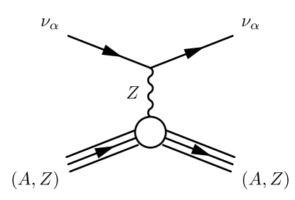
Figure 1: Feynman diagram illustrating the tree-level SM CE$\nu$NS process.

For sufficiently small momentum transfer, i.e. $q\leq 1/R$ where $R$ is the inverse nuclear radius , CE$\nu$NS dominates (see Fig. 1). In this case, only ground state to ground state ($g.s.\rightarrow g.s.$) transitions occur and lead to the following simplifications: the kinematics of the reaction imply $m_{f}=0$ and $|\mathbf{k}_{f}|=\varepsilon_{f}$ so that $a=1$ and $d=0$, while the momentum transfer can be cast in terms of the incoming neutrino energy $E_{\nu}$ in the simple form

$$Q^{2}=-q^{2}=4E^{2}_{\nu}\,\rm{sin}^{2}\frac{\theta}{2}\,,$$ (8)

where the usual notation $\varepsilon_{i}=\varepsilon_{f}\equiv E_{\nu}$ has been adopted. Note also that the excitation energy in this case is $\omega=0$ and $\kappa=\sqrt{-q^{2}}=\sqrt{Q^{2}}$, while angular momentum conservation implies that for CE$\nu$NS processes the only non-vanishing operator is the Coulomb, $T_{1}^{0}\equiv\hat{\mathcal{M}}_{0}^{0}$ (see the Appendix A.1 for the definition of the operators $T_{i}^{J}$). Then the corresponding differential cross section is further simplified and takes the form

$$\left(\frac{d\sigma}{d\rm{cos}\theta}\right)_{\text{SM}}=\frac{G_{F}^{2}}{2\pi}E_{\nu}^{2}\left(1+\rm{cos}\theta\right)|\langle g.s.||\hat{\mathcal{M}}_{0}^{0}(Q)||g.s.\rangle|^{2},$$ (9)

where the matrix element for $g.s.\rightarrow g.s.$ transitions is explicitly written in terms of the nuclear form factors for protons $F_{p}(Q^{2})$ and neutrons $F_{n}(Q^{2})$, as

$$\langle g.s.||\hat{\mathcal{M}}_{0}^{0}(Q)||g.s.\rangle=\frac{1}{2}\left[\left(1-4\rm{sin}^{2}\theta_{W}\right)Z\,F_{p}(Q^{2})-N\,F_{n}(Q^{2})\right]\,.$$ (10)

At CE$\nu$NS experiments the detection mechanism is sensitive to the tiny nuclear recoils generated in the aftermath of the scattering process. It is therefore reasonable to express the differential cross section with respect to the nuclear recoil energy $T_{N}$, which in the low energy approximation $T_{N}\ll E_{\nu}$, reads

$$\left(\frac{d\sigma}{dT_{N}}\right)_{\text{SM}}=\frac{G_{F}^{2}\,M}{4\pi}\left(1-\frac{M\,T_{N}}{2E_{\nu}^{2}}\right)|\langle g.s.||\hat{\mathcal{M}}_{0}^{0}(Q)||g.s.\rangle|^{2}\,,$$ (11)

where $T_{N}=Q^{2}/2M$ and $M$ is the mass of the nuclear isotope. The calculations of Ref. [61] involved the BCS form factors for protons (neutrons)

$$F_{N_{n}}=\frac{1}{N_{n}}\sum_{j}\sqrt{2j+1}\langle g.s.||j_{0}(\kappa r)||g.s.\rangle\left(v^{j}_{p(n)}\right)^{2}\,,$$ (12)

with $N_{n}=Z$ or $N$ and $v^{j}_{p(n)}$ represents the occupation probability amplitude of the $j$-th single nucleon level.

The method described above, involves realistic nuclear structure calculations making it more reliable compared to the use of phenomenological form factors, especially for accelerator neutrino sources (see the discussion in Subsect. II.2). For the reader’s convenience, Eq.(11) is also expressed through the vector weak nuclear charge $\mathcal{Q}_{W}^{V}$ in the approximation of equal proton and neutron form factors, as [69]

$$\left(\frac{d\sigma}{dT_{N}}\right)_{\text{SM}}=\frac{G_{F}^{2}\,M}{\pi}(\mathcal{Q}_{W}^{V})^{2}\left(1-\frac{M\,T_{N}}{2E_{\nu}^{2}}\right)F(Q)^{2}\,,$$ (13)

where the vector $\mathcal{Q}_{W}^{V}$ weak charge is given by [70]

$$\mathcal{Q}_{W}^{V}=\left[2(g_{u}^{L}+g_{u}^{R})+(g_{d}^{L}+g_{d}^{R})\right]Z+\left[(g_{u}^{L}+g_{u}^{R})+2(g_{d}^{L}+g_{d}^{R})\right]N\,,$$ (14)

with the left- and right-handed couplings of $u$ and $d$ quarks to the $Z$-boson being

$$g_{u}^{L}= \rho_{\nu N}^{NC}\left(\frac{1}{2}-\frac{2}{3}\hat{\kappa}_{\nu N}\hat{s}^{2}_{Z}\right)+\lambda^{u,L}\,,$$ (15)

$$g_{d}^{L}= \rho_{\nu N}^{NC}\left(-\frac{1}{2}+\frac{1}{3}\hat{\kappa}_{\nu N}\hat{s}^{2}_{Z}\right)+\lambda^{d,L}\,,$$

$$g_{u}^{R}= \rho_{\nu N}^{NC}\left(-\frac{2}{3}\hat{\kappa}_{\nu N}\hat{s}^{2}_{Z}\right)+\lambda^{u,R}\,,$$

$$g_{d}^{R}= \rho_{\nu N}^{NC}\left(\frac{1}{3}\hat{\kappa}_{\nu N}\hat{s}^{2}_{Z}\right)+\lambda^{d,R}\,.$$

The latter expressions include the radiative corrections from the PDG [71]: $\rho_{\nu N}^{NC}=1.0082$, $\hat{\kappa}_{\nu N}=0.9972$, $\lambda^{u,L}=-0.0031$, $\lambda^{d,L}=-0.0025$ and $\lambda^{d,R}=2\lambda^{u,R}=3.7\times 10^{-5}$ while concerning the weak mixing-angle the adopted value is $\hat{s}_{Z}^{2}\equiv\rm{sin}^{2}\theta_{W}=0.2382$. Regarding the incoherent neutrino-nucleus cross section and for the sake of completeness we note that apart from the Donnelly-Walecka method given in Eq.(2) a usefull formalism has been recently given in Ref. [62].

The differential cross sections $d\sigma/dT_{N}$ and $d\sigma/d\rm{cos}\theta$ are shown in the upper left and upper right panel of Fig. 2, from where it can be seen that large differences appear if the form factor dependence is neglected. On the other hand at low neutrino energies, i.e. $E_{\nu}\leq 20\,\mathrm{MeV}$ (relevant for reactor and solar neutrinos), the agreement of these two approximations is rather good. It is worth mentioning that forward scattering ($\theta=0$) leads to maximum $d\sigma/d\rm{cos}\theta$, as well as that for this particular case the form factor is by definition equal to unity due to the zero momentum transfer, see Eq.(8). Finally the bottom panel illustrates a comparison of the CE$\nu$NS cross section by incorporating the nuclear form factors and by assuming $F=1$.

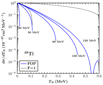
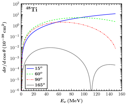
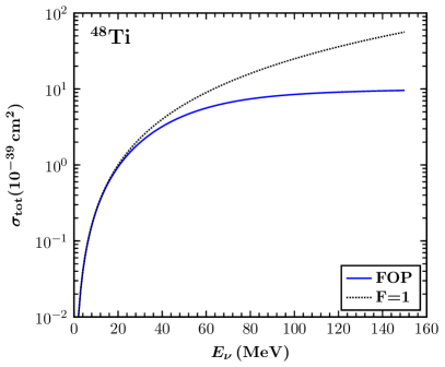
Figure 2: Upper Left: The differential cross section $d\sigma/dT_{N}$ in terms of the nuclear recoil energy $T_{N}$ for differenct incident neutrino energies. The results are compared to the case of point-like nucleus ($F=1$) for $E_{\nu}=50$ and $E_{\nu}=120$ MeV. Upper Right: The differential cross section $d\sigma/d\rm{cos}\theta$ as a function of the incoming neutrino energy $E_{\nu}$, for different scattering angles (for backward scattering the cross section vanishes). Bottom: The CE$\nu$NS cross section $\sigma_{\mathrm{tot}}$ as a function of the neutrino energy. An asymptotic behavior is found at neutrino energies $E_{\nu}\geq 80$ MeV or higher. Taken from Ref. [72].

II.2 Theoretical methods for obtaining the nuclear form factors

Electron scattering data provide high precision measurements of the proton charge density distribution [73]. The absence of similar data for neutron densities, restricts us to rely on the approximation of $\rho_{p}(\mathbf{r})=\rho_{n}(\mathbf{r})$ and thus assume $F_{p}(Q)=F_{n}(Q)\equiv F(Q)$ [see Eq.(13)]. In the context of nuclear theory, it is possible to treat separately the proton and neutron nuclear form factors by employing non-trivial techniques. The most reliable methods for this purpose include the large-scale Shell-Model [74, 75], the QRPA [76], Microscopic Quasiparticle Phonon Model (MQPM) [77], the deformed Shell-Model (DSM) method [39] and others. Recently, crucial information on important nuclear parameters has been extracted from the analysis of the recent COHERENT data in Refs. [32, 33, 34, 78].

The point-nucleon charge density distribution $\rho(\mathbf{r})$, is defined as the expectation value of the density operator [79]

$$\hat{\rho}(\mathbf{r})=\sum_{j=1}^{A}\frac{1}{2}(1\pm\tau_{3j})\delta(\mathbf{r}-\mathbf{r}_{j})\,,$$ (16)

where the $+$ ($-$) sign refers to the point-proton (neutron) charge density distribution. Assuming the nuclear ground state to be approximately described by a Slater determinant constructed from single-particle wavefunctions, the distributions of Eq.(16) are given by summing in quadrature the point-nucleon wavefunctions. According to Ref. [79], for closed (sub)shell nuclei the charge density distribution is assumed to be spherically symmetric while the interesting radial component ($r=|\mathbf{r}|$) of the proton charge density distribution, $\rho_{p}(r)$, can be cast in the form

$$\rho_{p}(r)=\frac{1}{4\pi}\sum_{\begin{subarray}{c}(n,l)j\\ \text{occupied}\end{subarray}}(2j+1)|R_{nlj}(r)|^{2}\,,$$ (17)

where $R_{nlj}(r)$ denotes the radial component of the single-particle wavefunction with quantum numbers $n$, $l$ and $j$. The nuclear form factor depends on the three momentum transfer squared $\mathbf{q}^{2}\equiv|\mathbf{q}|^{2}$ and can be obtained via a Fourier transformation

$$F_{p\,(n)}(\mathbf{q}^{2})=\frac{4\pi}{N_{n}}\int\rho_{p\,(n)}(r)j_{0}(|\mathbf{q}|r)\,r^{2}\,dr\,,\quad N_{n}=Z\,\,\text{or}\,\,N$$ (18)

where $j_{0}(x)=\rm{sin}x/x$ denotes the zero-order Spherical Bessel function of first kind. The nuclear form factors lead to a suppression of the CE$\nu$NS cross section and subsequently to a suppression of the expected event rates (see Ref. [32] for a comparison with the COHERENT data). The uncertainties of the nuclear form factors are explored in Ref. [35] where it is pointed out that studies looking for physics beyond the SM can be seriously affected by the uncertainty of the neutron form factor [80]. It is therefore important to treat with special care the nuclear form factors since new physics could be claimed or missed, if their uncertainties are not properly taken into account. In addition to the form factors obtained in the framework of the nuclear BCS method of Eq.(12), below we present a summary of various form factor approximations widely considered in the literature

i) Form factors from available electron-scattering experimental data
The proton nuclear form factors $F_{p}(\mathbf{q}^{2})$, may be evaluated through a model independent analysis (e.g. by employing a Fourier-Bessel expansion) of the electron scattering data [66], having however the disadvantage of assuming $F_{p}(\mathbf{q}^{2})=F_{n}(\mathbf{q}^{2})$.

ii) Fractional occupation probabilities (FOP) in a simple Shell-Model
For Harmonic Oscillator (h.o.) wavefunctions the nuclear form factor $F_{p}(\mathbf{q}^{2})$ for protons can be expressed in polynomial form [81, 82]

$$F_{p}(\mathbf{q}^{2})=\frac{1}{Z}e^{-(|\mathbf{q}|\,b)^{2}/4}\Phi\left(|\mathbf{q}|\,b,Z\right),\qquad\Phi\left(|\mathbf{q}|\,b,Z\right)=\sum_{\lambda=0}^{N_{\mathrm{max}}}\theta_{\lambda}(|\mathbf{q}|\,b)^{2\lambda}\,,$$ (19)

with $N_{\mathrm{max}}=(2n+l)_{\mathrm{max}}$ denoting for the number of quanta of the highest occupied proton (neutron) level. In a similar manner, the radial nuclear charge density distribution $\rho_{p}(r)$ is written in terms of the polynomials $\Pi\left(r/b,Z\right)$ in the following compact form [81, 82]

$$\rho_{p}(r)=\frac{1}{\pi^{3/2}b^{3}}e^{-(r/b)^{2}}\,\Pi\left(\frac{r}{b},Z\right),\qquad\Pi\left(\chi,Z\right)=\sum_{\lambda=0}^{N_{\mathrm{max}}}f_{\lambda}\chi^{2\lambda},$$ (20)

with the definition $\chi=r/b$ ($b$ stands for the h.o. size parameter). The explicit expressions for calculating the coefficients $\theta_{\lambda}$ and $f_{\lambda}$ are given in the Appendix A.2.

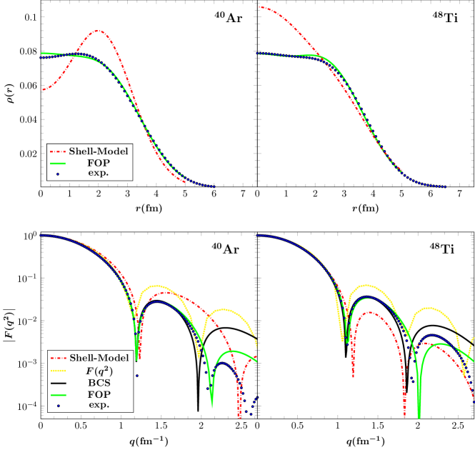
Figure 3: Charge density distribution (top) and nuclear form factor (bottom). The results refer to the ⁴⁰Ar and ⁴⁸Ti isotopes and are compared for different nuclear methods. Figure adapted from Ref. [61] under the terms of the Creative Commons Attribution 4.0 International license.

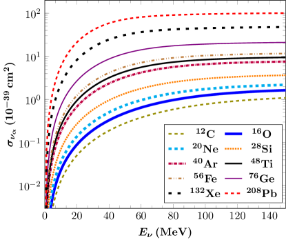
Figure 4: Integrated CE$\nu$NS cross sections $\sigma_{\nu_{\alpha}(\bar{\nu}_{\alpha})}(E_{\nu})$ for a set of nuclear targets ranging from light to heavy isotopes. Figure adapted from Ref. [61] under the terms of the Creative Commons Attribution 4.0 International license.

The occupation probabilities entering Eqs.(18) and (19) are assumed equal to unity (zero) for the states below (above) the Fermi surface, e.g. the filling numbers of the states for closed (sub)shell nuclei are those predicted by the simple Shell-Model. Going one step further, Ref. [79] introduced depletion/occupation numbers to describe the occupation probabilities of the surface levels, which satisfy the relation

$$\sum_{\begin{subarray}{c}(n,l)j\\ \mathrm{all}\end{subarray}}\alpha_{nlj}(2j+1)=N_{n}\,.$$ (21)

In this framework, there is a number of active surface nucleons (above or below the Fermi level) with non-vanishing occupation probability $0\leq\alpha_{nlj}\leq 1$ and a number of core levels with $\alpha_{nlj}=1$. The parameters are properly adjusted so that a high reproducibility of the experimental data is achieved [66]. By introducing four parameters $\alpha_{i},\,\,i=1,2,3,4$ in Eq.(21) the polynomial $\Pi(\chi,Z)$ of Eq.(20) reads

$$\Pi(\chi,Z,\alpha_{i})= \Pi(\chi,Z_{2})\frac{\alpha_{1}}{Z_{1}-Z_{2}}+\Pi(\chi,Z_{1})\left[\frac{\alpha_{2}}{Z_{c}-Z_{1}}-\frac{\alpha_{1}}{Z_{1}-Z_{2}}\right]$$ (22)

$$+\Pi(\chi,Z_{c})\left[\frac{Z^{\prime}-Z}{Z^{\prime}-Z_{c}}-\frac{\alpha_{2}}{Z_{c}-Z_{1}}-\frac{\alpha_{3}}{Z^{\prime}-Z_{c}}\right]$$

$$+\Pi(\chi,Z^{\prime})\left[\frac{Z-Z_{c}}{Z^{\prime}-Z_{c}}+\frac{\alpha_{3}}{Z^{\prime}-Z_{c}}-\frac{\alpha_{4}}{Z^{\prime\prime}-Z^{\prime}}\right]$$

$$+\Pi(\chi,Z^{\prime\prime})\left[\frac{\alpha_{4}}{Z^{\prime\prime}-Z^{\prime}}-\frac{\lambda}{Z^{\prime\prime\prime}-Z^{\prime\prime}}\right]+\Pi(\chi,Z^{\prime\prime\prime})\frac{\lambda}{Z^{\prime\prime\prime}-Z^{\prime\prime}}\,,$$

with $\lambda=\alpha_{1}+\alpha_{2}-\alpha_{3}-\alpha_{4}$ (see Ref. [61] for the fitted values).

iii) Use of effective expressions for the nuclear form factors
Besides calculations in the spirit of a nuclear structure model, a reliable description of the nuclear form factors (at least for low-energy reactor and solar neutrinos) may be obtained through the use of phenomenological approximations of the charge density distribution. The Helm-type density distribution is a convolution of a uniform nucleonic density with cut-off radius $R_{0}$ (accounting for the interior density) with a Gaussian falloff with folding width $s$ (surface thickness). The corresponding Helm form factor takes the analytical form as [83]

$$F_{\text{Helm}}(Q^{2})=3\frac{j_{1}(QR_{0})}{qR_{0}}\,e^{-(Qs)^{2}/2}\,,$$ (23)

where $j_{1}(x)=\frac{\rm{sin}x}{x^{2}}-\frac{\rm{cos}x}{x}$ is the 1st-order Spherical Bessel function. The first three moments can be analytically expressed as [84]

$$\left\langle R^{2}_{n}\right\rangle =\frac{3}{5}R_{0}^{2}+3s^{2}$$ (24)

$$\left\langle R^{4}_{n}\right\rangle =\frac{3}{7}R_{0}^{4}+6R_{0}^{2}s^{2}+15s^{4}$$

$$\left\langle R^{6}_{n}\right\rangle =\frac{1}{3}R_{0}^{6}+9R_{0}^{4}s^{2}+63R_{0}^{2}s^{4}+105s^{6}\,.$$

The surface thickness parameter is fixed to $s=0.9$ by fitting muon spectroscopy data [85], having also the advantage of improving the matching between the Helm and the symmetrized Fermi (SF) distributions [86]. The SF approximation follows from a Woods-Saxon charge density distribution and is expressed through the half density radius $c$ and the diffuseness parameter $a$, as [87]

$$F_{\text{SF}}\left(Q^{2}\right)=\frac{3}{Qc\left[(Qc)^{2}+(\pi Qa)^{2}\right]}\left[\frac{\pi Qa}{\sinh(\pi Qa)}\right]\left[\frac{\pi Qa\rm{sin}(Qc)}{\tanh(\pi Qa)}-Qc\rm{cos}(Qc)\right]\,,$$ (25)

with

$$c=1.23A^{1/3}-0.60\,\text{(fm)},\quad a=0.52\,\text{(fm)}\,,$$ (26)

while the surface thickness is written as $t=4a\ln 3$ [32]. The corresponding first three moments of the SF form factor read [84]

$$\left\langle R^{2}_{n}\right\rangle =\frac{3}{5}c^{2}+\frac{7}{5}(\pi a)^{2}$$ (27)

$$\left\langle R^{4}_{n}\right\rangle =\frac{3}{7}c^{4}+\frac{18}{7}(\pi a)^{2}c^{2}+\frac{31}{7}(\pi a)^{4}$$

$$\left\langle R^{6}_{n}\right\rangle =\frac{1}{3}c^{6}+\frac{11}{3}(\pi a)^{2}c^{4}+\frac{239}{15}(\pi a)^{4}c^{2}+\frac{127}{5}(\pi a)^{6}\,.$$

The Klein-Nystrand (KN) distribution is obtained from the convolution of a Yukawa potential with range $a_{k}=0.7$ fm over a Woods-Saxon distribution (hard sphere with radius $R_{A}$). The resulting KN form factor reads [88]

$$F_{\text{KN}}=3\frac{j_{1}(QR_{A})}{QR_{A}}\left[1+(Qa_{k})^{2}\right]^{-1}\,,$$ (28)

and is adopted by the COHERENT Collaboration, while in this case root mean square (rms) radius reads

$$\langle R^{2}_{n}\rangle_{\text{KN}}=3/5R_{A}^{2}+6a_{k}^{2}\,.$$ (29)

Fig. 3 presents the charge density distribution in the top panel and the corresponding nuclear form factors for ⁴⁰Ar (interesting for LAr CE$\nu$NS detectors) and ⁴⁸Ti (interesting for $\mu^{-}\to e^{-}$ conversion in nuclei) in the lower panel, while the results are compared for the various methods used. A comparison of the form factors for ¹²⁷I and ¹³³Cs that are of interest for COHERENT, evaluated with the DSM method (not covered here), with those of the Helm, SF and KN parametrizations, is given in Ref. [36]. By incorporating realistic nuclear structure calculations on the basis of the BCS method, the SM CE$\nu$NS cross section is given in Fig. 4 for a set of different isotopes throughout the periodic table. For heavier isotopes the form factor suppression is more pronounced and therefore the cross sections flatten more quickly, since the nuclear effects become significant even at low-energies.

III Constraints within and beyond the SM from CE$\nu$NS

The observation of CE$\nu$NS by the COHERENT experiment with a $\pi$-DAR neutrino source is a portal to new physics triggering a considerable number of phenomenological studies at low-energies. New constraints have been put on neutrino, electroweak and nuclear physics parameters, that we devote an effort to summarize below. The experimental confirmation of CE$\nu$NS has also prompted a great rush in the experimental physics community and several projects are aiming to measure CE$\nu$NS using reactor neutrinos from nuclear power plants (NPP). It should be stressed that given the large potential of improvement in detector technology and control of systematics, it is feasible to further explore the low-energy and precision neutrino frontier. The CONUS experiment is currently running at the Brokdorf NPP (Germany) and has already released preliminary results while the COHERENT experiment has released new results from the engineering run with a LAr detector [89]. Moreover, a number of prominent experiments are in preparation such as: the MINER experiment at the TRIGA Nuclear Science Center at Texas A&M University (USA), the CONNIE project at the Angra NPP (Brazil), the NUCLEUS and Ricochet experiments at the Chooz NPP (France) , the TEXONO program at the Kuo-Sheng NPP (Taiwan), the vGEN and RED100 experiments at the Kalinin NPP (Russia), the Coherent Captain-Mills (CCM) project at Los Alamos Neutron Science Center (LANSCE) as well as new proposals for a CE$\nu$NS measurement by employing a ⁵¹Cr source [91] and new posibilities in China  (an exhaustive review of the CE$\nu$NS experimental developments is given in Ref. [60]). Finally, it has been recently discussed the possibility of measuring CE$\nu$NS at the European Spallation Source (ESS) [92]. Table 1 lists a summary of the current and future experimental projects, while Fig. 5 demonstrates the differential event rate for the various target nuclei at $\pi$-DAR (see Ref. [93]) and at the various reactor CE$\nu$NS experiments neglecting detector efficiencies and quenching factors (QF).

In reality however, these experiments are sensitive to an ionization energy (e.g. electron equivalent energy $\mathrm{eV_{ee}}$) since a large portion of the nuclear recoil energy $\mathrm{eV_{nr}}$ is lost to heat (conversion to phonons). The energy discrepancy has to be determined experimentally and is taken into account in terms of the QF. The latter quantity is crucial for such processes and depends on the nuclear recoil energy as well as on the target nucleus in question. Theoretically it follows the empirical form arising from the Lindhard theory [86]

$$\mathsf{Q}(T_{N})=\frac{\kappa g(\gamma)}{1+\kappa g(\gamma)}\,,$$ (30)

with $g(\gamma)=3\gamma^{0.15}+0.7\gamma^{0.6}+\gamma$ and $\gamma=11.5\,T_{N}(\text{keV})Z^{-7/3}$, $\kappa=0.133\,Z^{2/3}A^{-1/2}$. The left and right panels of Fig. 6 quantify the effect of the QF in the case of CE$\nu$NS .

Experiment	$T_{\text{th}}$	Baseline (m)	Target	Mass (kg)	Technology	Source
COHERENT [94]	6.5 keV	19.3	CsI[Na]	14.57	Scintillating crystal	$\pi$-DAR SNS
	5 keV	22	Ge	10	HPGe PPC
	20 keV	29	LAr	$2\times 10^{3}$	Single phase
	13 keV	28	NaI[Tl]	185*/3388	Scintillating crystal
CCM [95]	10-20 keV	20-40	LAr	$10^{4}$	Scintillation	$\pi$-DAR Lujan
CONUS [96]	300 eV	17	Ge	4	HPGe	NPP 3.9 GW
MINER [47]	10 eV	1	Ge/Si	30	cryogenic	NPP 1 MW
CONNIE [97]	28 eV	30	Si	1	Si CCDs	NPP 3.8 GW
Ricochet [50]	50-100 eV	<10	Ge/Zn	10	Ge, Zn bolometers	NPP 8.54 GW
NUCLEUS [98]	20 eV	<10	$\mathrm{CaWO_{4}}$ $\mathrm{Al_{2}O_{3}}$	$10^{-3}$	Cryogenic $\mathrm{CaWO_{4}}$ $\mathrm{Al_{2}O_{3}}$ calorimeter array	NPP 8.54 GW
RED100 [99]	500 eV	19	Xe	100	LXe dual phase	NPP 3 GW
vGEN	350 eV	10	Ge	4 $\times$ 0.4	Ge PPC	NPP 3 GW
TEXONO [100]	150-200 eV	28	Ge	1	p-PCGe	NPP 2 $\times$ 2.9 GW

Table 1: Current and future experimental proposals for CE$\nu$NS searches.

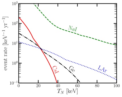
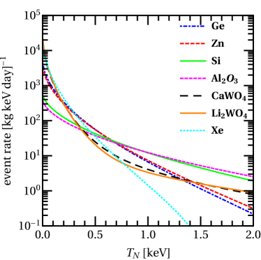
Figure 5: Expected CE$\nu$NS event rate for the different detector subsystems of the COHERENT experiment (left) and for the different target nuclei relevant to reactor based experiments (right). For the case of COHERENT the results are shown according to the setups of Table 1, while for reactor based experiments the calculation assumes 1 kg of each target located at 20 m from a 4 GW reactor NPP. The impact of QF and efficiency is ignored.

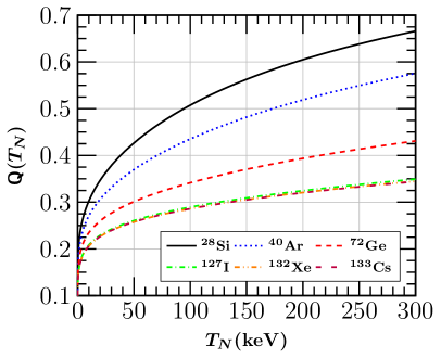
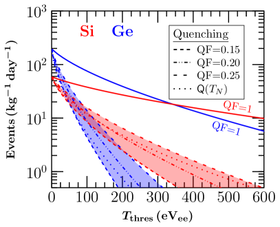
Figure 6: Left: The QF as a function of the nuclear recoil energy. Right: the impact of the QF on the expected number of events at a reactor based experiment assuming a typical neutrino flux of $10^{13}\,\mathrm{cm^{-2}s^{-1}}$ for CE$\nu$NS off Silicon and Germanium detectors. The figure in the left panel has been adapted from Ref. [22] under the terms of the Creative Commons Attribution 4.0 International license.

III.1 Electroweak and nuclear physics

The left panel of Fig. 7 shows the expected number of events at the CsI[Na] detector of COHERENT and gives a comparison with the experimental data, from where it can be seen that a good agreement is reached. In Ref. [21] the authors analyzed the CE$\nu$NS data and obtained a low-energy determination of the weak mixing angle, as illustrated in the right panel of Fig. 7. The obtained constraint at 90% C.L. reads [21]

$$\rm{sin}^{2}\theta_{W}=0.197^{+0.128}_{-0.080}\,.$$ (31)

An interesting analysis combining atomic parity violating (APV) and CE$\nu$NS data was performed in Ref. [101], while the prospects regarding the future reactor-based CE$\nu$NS experiments such as those presented in Table 1, have been extracted in Ref. [102]. On the other hand, an improved determination of the CsI[Na] quenching factor can in principle lead to a significantly better agreement between the experimental results and the theoretical simulations [103], as well as to an improved sensitivity on the weak mixing angle [78].

The discussion made in the previous Section emphasized how the CE$\nu$NS cross section depends on the nuclear physics effects which are incorporated through the momentum variation of the relevant nuclear form factor. The authors of Ref. [27] demonstrated how the intrinsic nuclear structure uncertainties may have a significant impact to searches beyond the SM such those regarding NSIs, sterile neutrinos and neutrino generalized interactions (GNIs). Starting from the form factor of Eq.(18) and expanding in terms of even moments of the charge density distribution one arrives to a model independent expression [104]

$$F_{p,n}(Q^{2})\approx 1-\frac{Q^{2}}{3!}\langle R_{p,n}^{2}\rangle+\frac{Q^{4}}{5!}\langle R_{p,n}^{4}\rangle-\frac{Q^{6}}{7!}\langle R_{p,n}^{6}\rangle+\cdots\,,$$ (32)

with the $k$-th radial moment defined as

$$\langle R_{p,n}^{k}\rangle=\frac{\int\rho_{p,n}(\vec{r})\,r^{k}\,d^{3}\vec{r}}{\int\rho_{p,n}(\vec{r})\,d^{3}\vec{r}}\,,$$ (33)

allowing the study of contributions of higher-order moments to nuclear form factors [33]. A sensitivity analysis of the two first moments with current and future COHERENT data is depicted in Fig. 8 where the allowed regions are presented at 1$\sigma$, 90% and 99% C.L. The calculation in this case was restricted in the physical region [0,6] fm in order to obey the upper limit on $R_{n}(^{208}\text{Pb})=5.75\pm 0.18$ fm from the PREM experiment [105]. The future scenarios considered assume improved statistical uncertainties and more massive detectors in accord with the next generation COHERENT experiments [94] (see Ref. [36] for details), while as demonstrated in Ref. [104] multi-ton scale detectors will provide significant improvements.

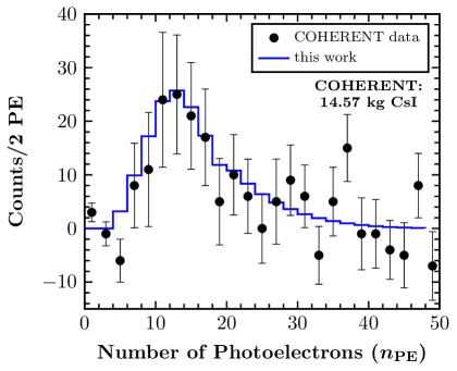
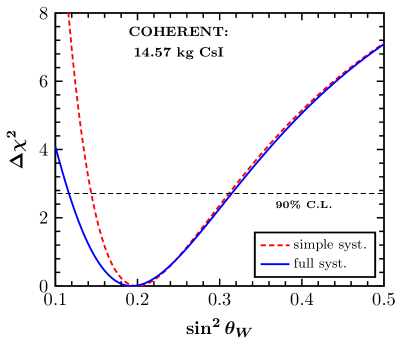
Figure 7: Comparison between the simulated number of CE$\nu$NS events and the experimental data by COHERENT (left) and sensitivity of COHERENT on the weak mixing angle (right). Figure adapted from Ref. [21] under the terms of the Creative Commons Attribution 4.0 International license.

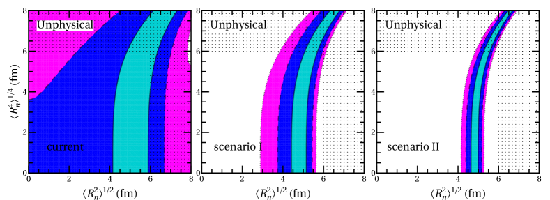
Figure 8: Sensitivity contours in the $\langle R_{n}^{2}\rangle^{1/2}$–$\langle R_{n}^{4}\rangle^{1/4}$ plane from the COHERENT data assuming the current and possible future detector specifications (see the text). The allowed regions are shown at $1\sigma$ (turquoise), 90% C.L. (blue) and 99% C.L. (magenta). Taken from Ref. [36].

The average CsI neutron rms radius has been explored in Refs. [32, 36, 34] using the energy spectrum of the available CE$\nu$NS data. The corresponding sensitivity profiles are presented in Fig. 9, leading to the best fits at 90% C.L. [36]

$$\langle R_{n}^{2}\rangle^{1/2}= 5.64^{+0.99}_{-1.23}\,\text{fm}\quad\text{(current)}\,,$$ (34)

$$\langle R_{n}^{2}\rangle^{1/2}= 5.23^{+0.42}_{-0.50}\,\text{fm}\quad\text{(scenario I)}\,,$$

$$\langle R_{n}^{2}\rangle^{1/2}= 5.23^{+0.22}_{-0.22}\,\text{fm}\quad\text{(scenario II)}\,,$$

while the potential of improvement through a more accurate determination of the QF is promising (see e.g. Ref. [78]). An independent analysis combining APV and CE$\nu$NS data was perfomed in Ref. [106] leading to essentially similar results. Finally, it is worthwhile to mention the reported upper bound on the neutron skin $\Delta R_{np}=\Delta R_{n}-\Delta R_{p}=0.7^{+0.9}_{-1.1}$ fm [32].

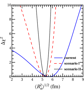
Figure 9: COHERENT sensitivity on the average nuclear rms radius of CsI assuming the current and possible future detector spesifications. Taken from Ref. [36].

III.2 Nonstandard and generalized neutrino interactions

Non-standard interactions (NSI) [107] apperar in several appealing SM extensions [108] involving four-fermion contact interaction, various seesaw realizations [109, 110, 111], left-right symmetry [112], gluonic operators [113], etc., constituting an interesting model independent probe of new physics. NSIs may have implications to SN [114], neutrino oscillations [57] and CE$\nu$NS  [70, 115], while recently NSI terms were explored in the context of GNI [116] and effective field theory (EFT) operators [117, 118]. Finally the RG issue has been partly addressed in the context of NSI in Ref. [119].

For sufficiently low energies vector-type NSIs arise from the effective four-fermion operators [56]

$$\mathcal{O}_{\alpha\beta}^{qV}=\left(\bar{\nu}_{\alpha}\gamma^{\mu}L\nu_{\beta}\right)\left(\bar{q}\gamma_{\mu}Pq\right)+\mathrm{H.c.}\,,$$ (35)

leading to new contributions to the CE$\nu$NS rate from exotic processes of the form

$$\nu_{\alpha}(\bar{\nu}_{\alpha})+(A,Z)\rightarrow\nu_{\beta}(\bar{\nu}_{\beta})+(A,Z)\,,$$ (36)

where $\alpha,\beta=\{e,\mu,\tau$} ($\alpha\neq\beta$), $q$ denotes a first-generation quark $q=\{u,d\}$ and $P=\{L,R\}$ is the chiral projection operator. For the case of CE$\nu$NS the new interactions are taken into account through the NSI charge with the substitution $\mathcal{Q}_{W}^{V}\rightarrow\mathcal{Q}_{\mathrm{NSI}}^{V}$ in Eq.(14). The latter contains flavor-preserving non-universal ($\epsilon_{\alpha\alpha}^{qV}$) and flavor changing ($\epsilon_{\alpha\beta}^{qV}$) terms and is expressed as

$$\mathcal{Q}_{\mathrm{NSI}}^{V}= (2\epsilon_{\alpha\alpha}^{uV}+\epsilon_{\alpha\alpha}^{dV}+g^{V}_{p})Z+(\epsilon_{\alpha\alpha}^{uV}+2\epsilon_{\alpha\alpha}^{dV}+g^{V}_{n})N$$ (37)

$$+\sum_{\alpha\neq\beta}\left[(2\epsilon_{\alpha\beta}^{uV}+\epsilon_{\alpha\beta}^{dV})Z+(\epsilon_{\alpha\beta}^{uV}+2\epsilon_{\alpha\beta}^{dV})N\right]\,,$$

implying that the NSI CE$\nu$NS cross section becomes flavor dependent.

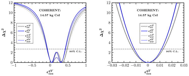
Figure 10: Sensitivity of COHERENT to vector (left) and tensor (right) NSI parameters. Thick (thin) curves correspond to the $\nu_{e}$ ($\nu_{\mu}+\bar{\nu}_{\mu}$) beam. Figure adapted from Ref. [21] under the terms of the Creative Commons Attribution 4.0 International license.

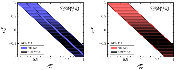
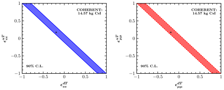
Figure 11: Sensitivity contours in the vector (upper panel) and tensor (lower panel) NSI parameter space. The results are presented at 90% C.L. assuming non-universal couplings only. The left (right) panel corresponds to the $\nu_{e}$ ($\nu_{\mu}+\bar{\nu}_{\mu}$) beam, while the best-fit points are indicated by an asterisk $\star$. Figure adapted from Ref. [21] under the terms of the Creative Commons Attribution 4.0 International license.

There is a reach literature on NSI investigations with the recent COHERENT data. Assuming one nonvanishing coupling at a time, the authors of Ref. [21] focused on the non-universal terms and obtained the sensitivity profiles shown in the left panel of Fig. 10, while the corresponding allowed regions resulting from a combined analysis of the NSI couplings are illustrated in the upper panel of Fig. 11 at 90% C.L. Regarding the future prospects of MINER, Ricochet, NUCLEUS and CONNIE, similar studies were conducted concentrating on the non-universal [120] and flavor-changing [121] terms. Indeed, a multitarget strategy can break degeneracies involved between up and down flavor-diagonal NSI terms that survives analysis of neutrino oscillation experiments [14]. Constraints on the corresponding parameters arising from leptoquarks [120], GNI [116] and EFT [117, 118] have been also reported. NSI constraints from CE$\nu$NS place meaningfull constraints excluding a large part of the existing CHARM constraints and overlap with results coming out of LHC monojet searches (see Ref. [120] for a usefull comparison). Regarding the near-term future, a potential improvement on determination of the QF [103] may yield severe constraints. For example, updated bounds are possible by analyzing the number of events [78], the energy spectrum [122] as well as through a combined analysis of both energy and timing COHERENT data [123].

Novel tensor-type interactions are predicted in the general context of NSI [124] and GNI [116] which induce terms of the form

$$\mathcal{O}_{\alpha\beta}^{qT}=\left(\bar{\nu}_{\alpha}\sigma^{\mu\nu}\nu_{\beta}\right)\left(\bar{q}\sigma_{\mu\nu}q\right)+\mathrm{H.c.}$$ (38)

Such interactions violate the chirality constraint allowing for a wide class of new interactions, e.g. relevant to neutrino EM properties (see Ref. [125, 126]). Contrary to the vector NSI case, for tensorial interactions there is absence of interference with the SM interactions. In the approximation of a vector-type translation the corresponding tensor NSI charge has been expressed as [124]

$$\mathcal{Q}_{\mathrm{NSI}}^{T}=(2\epsilon_{\alpha\alpha}^{uT}+\epsilon_{\alpha\alpha}^{dT})Z+(\epsilon_{\alpha\alpha}^{uT}+2\epsilon_{\alpha\alpha}^{dT})N\,,$$ (39)

while a more systematic interpetation has been carried out in Ref. [116]. To account for the new contributions in the presence of tensorial NSI, the CE$\nu$NS cross is written [21]

$$\left(\frac{d\sigma}{dT_{N}}\right)_{\mathrm{SM+NSI_{tensor}}}=\mathcal{G}_{\mathrm{NSI}}^{T}(E_{\nu},T_{N})\left(\frac{d\sigma}{dT_{N}}\right)_{\mathrm{SM}}\,,$$ (40)

with the tensor NSI factor defined as

$$\mathcal{G}_{\mathrm{NSI}}^{T}=1+4\left(\frac{\mathcal{Q}_{\mathrm{NSI}}^{T}}{\mathcal{Q}_{W}^{V}}\right)^{2}\frac{1-\frac{MT_{N}}{4E_{\nu}^{2}}}{1-\frac{MT_{N}}{2E_{\nu}^{2}}}\,.$$ (41)

From the analysis of the COHERENT data, the sensitivity profiles accounting to tensor NSIs, assuming one non-zero coupling at a time, are illustrated in the right panel of Fig. 10 (see also Ref. [21]). The corresponding allowed regions coming out from a two parameter analysis are presented in the lower panel of Fig. 11 at 90% C.L. The result is more stringent as compared to the analysis carried out in the framework of GNI for reasons discussed above. On the other hand, comparing with the vector NSI case the absence of SM-tensor NSI interference causes the allowed regions to appear with more narrow bands.

III.3 The Novel NSI mediators $Z^{\prime}$ (vector) and $\phi$ (scalar)

Theories beyond the SM with an additional $\mathrm{U(1)}^{\prime}$ symmetry have been comprehensively investigated. Regarding CE$\nu$NS related studies a novel massive mediator predicted in these concepts is expected to induce a detectable distortion to the nuclear recoil spectrum, provided that its mass is comparable to the momentum transfer. The study of models with new vector or scalar interactions that involve hidden sector particles may be also accessible at CE$\nu$NS experiments [127]. Such frameworks are interesting since they may play a central role in explaining anomalies with regards to $B$-meson decays at the LHCb experiment [128] and at DM searches [129].

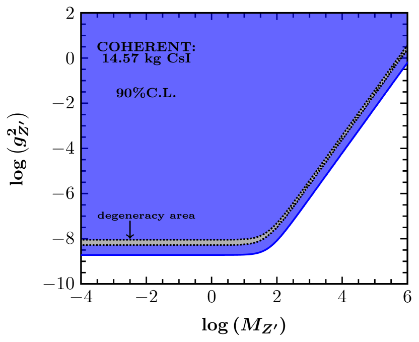
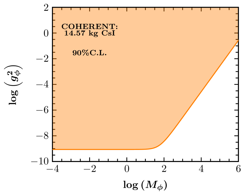
Figure 12: Excluded regions at 90% C.L. by the COHERENT experiment assuming simplified scenarios involving a $Z^{\prime}$ vector mediator (left panel) and a $\phi$ scalar mediator (right panel). The mediator masses are in units of MeV. Figure adapted from Ref. [21] under the terms of the Creative Commons Attribution 4.0 International license.

We first examine the case of a new massive vector boson $Z^{\prime}$. Restricting ourselves to the neutrino sector with only left-handed neutrinos the Lagrangian reads [130]

$$\mathcal{L}_{\mathrm{vec}}=Z^{\prime}_{\mu}\left(g_{Z^{\prime}}^{qV}\bar{q}\gamma^{\mu}q+g_{Z^{\prime}}^{\nu V}\bar{\nu}_{L}\gamma^{\mu}\nu_{L}\right)+\frac{1}{2}M_{Z^{\prime}}^{2}Z^{\prime}_{\mu}Z^{\prime\mu}\,.$$ (42)

The arising cross sections imply a re-scaling of the SM one according to the expression

$$\left(\frac{d\sigma}{dT_{N}}\right)_{\mathrm{SM}+Z^{\prime}}=\mathcal{G}_{Z^{\prime}}^{2}(T_{N})\left(\frac{d\sigma}{dT_{N}}\right)_{\mathrm{SM}}\,,$$ (43)

with the $Z^{\prime}$ factor taking the form

$$\mathcal{G}_{Z^{\prime}}=1-\frac{1}{2\sqrt{2}G_{F}}\frac{\mathcal{Q}_{Z^{\prime}}}{\mathcal{Q}_{W}^{V}}\frac{g_{Z^{\prime}}^{\nu V}}{2MT_{N}+M_{Z^{\prime}}^{2}}\,.$$ (44)

Here, $g_{Z^{\prime}}^{\nu V}$ denotes the neutrino-vector coupling, while the respective $Z^{\prime}$ charge reads [129]

$$\mathcal{Q}_{Z^{\prime}}=\left(2g^{uV}_{Z^{\prime}}+g^{dV}_{Z^{\prime}}\right)Z+\left(g^{uV}_{Z^{\prime}}+2g^{dV}_{Z^{\prime}}\right)N\,.$$ (45)

However, in the general case the $\nu-Z^{\prime}$ coupling is flavor dependent $(g_{Z^{\prime}}^{\nu V})_{\alpha\beta}$. Ref. [16] has explored this possibility and concluded that for a sufficiently small momentum transfer with respect to $M_{Z^{\prime}}$, the new physics contributions can be addressed in the form of NSIs

$$\epsilon_{\alpha\beta}^{qV}=\frac{(g_{Z^{\prime}}^{\nu V})_{\alpha\beta}\,g^{qV}}{2\sqrt{2}G_{F}M^{2}_{Z^{\prime}}}\,,$$ (46)

where the $Z^{\prime}$ has been integrated out. Unlike the NSI case that can only modify the energy spectrum by a global factor, the additional momentum dependence expected due to the new light mediators discussed here can be well encoded in the detected signature and subsequently lead to conclusive indications of the new physics nature.

We now turn our attention on new interactions induced by the presence of a CP-even mediator. In particular, we consider a new real scalar boson $\phi$ with mass $M_{\phi}$, based on the Lagrangian [130]

$$\mathcal{L}_{\mathrm{sc}}=\phi\left(g_{\phi}^{qS}\bar{q}q+g_{\phi}^{\nu S}\bar{\nu}_{R}\nu_{L}+\mathrm{H.c.}\right)-\frac{1}{2}M_{\phi}^{2}\phi^{2}\,,$$ (47)

with $g_{\phi}^{qS}$ and $g_{\phi}^{\nu S}$ representing the scalar-quark and scalar-neutrino couplings, respectively. In this framework the SM CE$\nu$NS cross section acquires an additive contribution due to the boson exchange that can be quantified in terms of the respective cross section

$$\left(\frac{d\sigma}{dT_{N}}\right)_{\mathrm{scalar}}=\frac{G_{F}^{2}M^{2}}{4\pi}\frac{\mathcal{G}_{\phi}^{2}M_{\phi}^{4}T_{N}}{E_{\nu}^{2}\left(2MT_{N}+M_{\phi}^{2}\right)^{2}}F^{2}(T_{N})\,,$$ (48)

with the scalar factor $\mathcal{G}_{\phi}$ being

$$\mathcal{G}_{\phi}=\frac{g^{\nu S}_{\phi}\mathcal{Q}_{\phi}}{G_{F}M_{\phi}^{2}}\,.$$ (49)

Analogously to the previous case, the corresponding scalar charge is defined as [130]

$$\mathcal{Q}_{\phi}=\sum_{\mathcal{N},q}g^{qS}_{\phi}\frac{m_{\mathcal{N}}}{m_{q}}f_{T,q}^{(\mathcal{N})}\,,$$ (50)

where the form factors $f_{T,q}^{(\mathcal{N})}$ capture the effective low-energy coupling of $\phi$ to the nucleon $\mathcal{N}=\{p,n\}$ ($m_{\mathcal{N}}$ is the nucleon mass) for the quark $q$.

As discussed previously, different new physics signatures are expected to leave different imprints on the event and recoil spectrum. Contrary to the $Z^{\prime}$ scenario discussed above, the Dirac structure of the $\phi\bar{\nu\nu}$ vertex accounting for the scalar mediator is different (chirality-flipping) with respect to the SM one (chirality-conserving). Indeed, there is no interference between vector (or axial-vector) neutrino interactions and (pseudo-)scalar, tensor neutrino interactions [131, 29]. Therefore, the absence of interference between SM-scalar interactions gives rise to an overall modification of the expected CE$\nu$NS spectrum (see Ref. [129]). Moreover, comparing the vector and scalar cross sections it becomes evident that the corresponding signals are expected to be well distinguishable. The scalar effects are not pronounced at eV-thresholds, while on the contrary they are expected to be stronger at recoil energies of the order of keV. A thorough classification of the new physics signatures with respect to vector and scalar interactions is given in Ref. [132] providing also key information on the possibility of breaking isospin-related degeneracies from combined measurements with different detector material.

Assuming universal couplings, one finds the equalities [130]

$$g_{Z^{\prime}}^{2}=\frac{g^{\nu V}_{Z^{\prime}}\mathcal{Q}_{Z^{\prime}}}{3A}\,,\quad g_{\phi}^{2}=\frac{g^{\nu S}_{\phi}\mathcal{Q}_{\phi}}{\left(14A+1.1Z\right)}\,.$$ (51)

Using the COHERENT data, bounds have been put on the parameter planes $(g_{Z^{\prime}}^{2},M_{Z^{\prime}})$ and $(g_{\phi}^{2},M_{\phi})$ for the vector and scalar mediators, respectively [21]. In the left panel of Fig. 12, the limits are shown at 90% C.L., where a degenerate area appears that cannot be excluded by the data is found due to the cancellations involved in Eq.(44). However as shown in Ref. [13] this degeneracy can be broken in the context of NSI, while for heavy mediator masses, $M_{Z^{\prime}}\gg\sqrt{2MT_{N}}\sim 50~{}\mathrm{MeV}$, it remains unbroken and depends on the ratio

$$\frac{g^{2}_{Z^{\prime}}}{M^{2}_{Z^{\prime}}}\approx 2\sqrt{2}G_{F}\frac{\mathcal{Q}_{W}^{V}}{3A}\,.$$ (52)

For the case of light mediator masses $M_{Z^{\prime}}\ll\sqrt{2MT_{N}}$, it holds

$$g^{2}_{Z^{\prime}}\approx 4\sqrt{2}G_{F}\frac{\mathcal{Q}_{W}^{V}}{3A}MT_{N}\,,$$ (53)

which implies that the bound is only sensitive to the coupling. The latter could be drastically improved by combining data from different detectors [133]. The case of a scalar field mediating CE$\nu$NS is explored in the right panel of Fig. 12 where the extracted bounds in the $(M_{\phi},g_{\phi}^{2})$ plane are depicted at 90% C.L. Significant improvements are possible through powerful analyses that are based on both energy and timing COHERENT data [17] as well as by taking into account improved quenching factors [78]. The future of CE$\nu$NS experiments will offer a complementary probe to various existing limits in the low- and high-energy regime. The currently best results for a low-energy light vector mediator of $M_{Z^{\prime}}<10~{}\mathrm{MeV}$ have been recently reported by the CONNIE Collaboration [134]. The attainable sensitivity is expected to be competitive with existing bounds from neutrino-electron scattering, dark photon searches at BaBar and LHCb results (see Refs. [30, 120]). Before closing our discussion it is important to note that, very recently CP violating effects have been also analyzed with the current and future COHERENT data in the context of light vector mediator scenarios [27]. The latter have been also found to be applicable to reactor or solar/atmospheric neutrino searches with important implications on multi-ton dark matter detectors.

III.4 Studying electromagnetic neutrino interactions

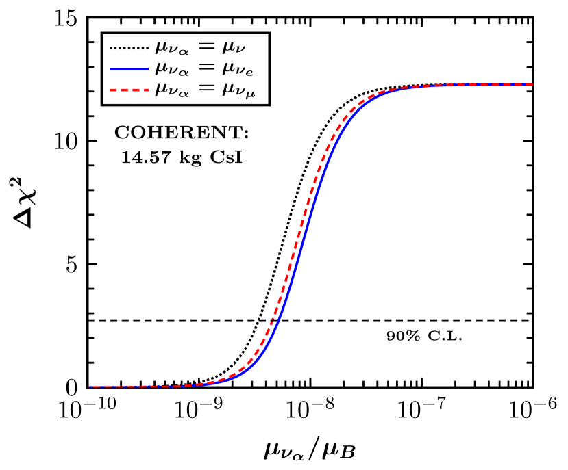
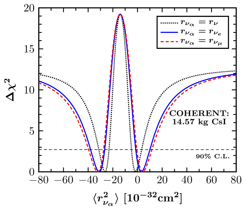
Figure 13: Constraints on electromagnetic neutrino properties by the COHERENT experiment. Left: sensitivity to the effective neutrino magnetic moment $\mu_{\nu_{\alpha}}$. Right: sensitivity to the neutrino charge-radius $\langle r_{\nu_{\alpha}}^{2}\rangle$. Figure adapted from Ref. [21] under the terms of the Creative Commons Attribution 4.0 International license.

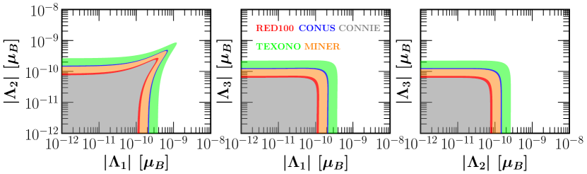
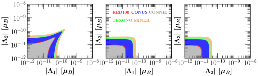
Figure 14: Sensitivity contours at 90% C.L. in the $\left|\Lambda_{i}\right|-\left|\Lambda_{j}\right|$ parameter space that follow from the expected results of the current and future reactor based CE$\nu$NS experiments (see the text). The calculation assumes vanishing $\left|\Lambda_{k}\right|$ and vanishing CP phases $\zeta_{i}$. Figure adapted from Ref. [22] under the terms of the Creative Commons Attribution 4.0 International license.

Non-trivial electromagnetic (EM) properties of massive neutrinos constitute an interesting probe to look for physics beyond the SM and at the same time they are crucial for distinguishing between the Dirac or Majorana nature of neutrinos [135]. The two main phenomenological parameters observable at a neutrino experiment are the effective neutrino magnetic moment and the neutrino charge radius (the possibility of a neutrino millicharge is explored in Refs. [23, 106]). Assuming Majorana neutrinos, the EM neutrino vertex is described by the electromagnetic field tensor $F_{\alpha\beta}$ of the effective Hamiltonian [136, 3]

$$H_{\text{EM}}^{\mathrm{M}}=-\frac{1}{4}\nu_{L}^{\mathsf{T}}C^{-1}\lambda\sigma^{\alpha\beta}\nu_{L}F_{\alpha\beta}+\mathrm{H.c.}\,,$$ (54)

while for the case of Dirac neutrinos one has

$$H_{\text{EM}}^{\mathrm{D}}=\frac{1}{2}\bar{\nu}_{R}\lambda\sigma^{\alpha\beta}\nu_{L}F_{\alpha\beta}+\mathrm{H.c.}$$ (55)

It is important to note that for Majorana (Dirac) neutrinos $\lambda=\mu-i\epsilon$ is an antisymmetric complex (general complex) matrix. The two imaginary matrices $\mu$ (magnetic moment) and $\epsilon$ (electric dipole moment) obey the respective properties $\mu^{\mathsf{T}}=-\mu$ ($\mu=\mu^{\dagger}$) while $\epsilon^{\mathsf{T}}=-\epsilon$ ($\epsilon=\epsilon^{\dagger}$). It thus becomes evident that, unlike the Dirac case, for Majorana neutrinos the diagonal moments are vanishing $\mu^{\mathrm{M}}_{ii}=\epsilon^{\mathrm{M}}_{ii}=0$.

For a low-energy neutrino scattering experiment the observable neutrino magnetic moment (flavor dependent) is in fact a combination of the neutrino transition magnetic moments (TMMs) discussed above. In the mass basis it reads [137]

$$\left(\mu_{\nu}^{M}\right)^{2}=\tilde{\mathfrak{a}}_{-}^{\dagger}\tilde{\lambda}^{\dagger}\tilde{\lambda}\tilde{\mathfrak{a}}_{-}+\tilde{\mathfrak{a}}_{+}^{\dagger}\tilde{\lambda}\tilde{\lambda}^{\dagger}\tilde{\mathfrak{a}}_{+}\,.$$ (56)

In Eq.(56) the following transformations have been introduced

$$\tilde{\mathfrak{a}}_{-}=U^{\dagger}\mathfrak{a}_{-},\qquad\tilde{\mathfrak{a}}_{+}=U^{\mathsf{T}}\mathfrak{a}_{+},\qquad\tilde{\lambda}=U^{\mathsf{T}}\lambda U\,,$$ (57)

where the $3-$vectors $\mathfrak{a}_{+}$ and $\mathfrak{a}_{-}$ denote positive and negative helicity states respectively, while the magnetic moment matrix $\lambda$ ($\tilde{\lambda}$) in the flavor (mass) basis is written as [138]

$$\lambda=\left(\begin{array}[]{ccc}0&\Lambda_{\tau}&-\Lambda_{\mu}\\ -\Lambda_{\tau}&0&\Lambda_{e}\\ \Lambda_{\mu}&-\Lambda_{e}&0\end{array}\right),\qquad\tilde{\lambda}=\left(\begin{array}[]{ccc}0&\Lambda_{3}&-\Lambda_{2}\\ -\Lambda_{3}&0&\Lambda_{1}\\ \Lambda_{2}&-\Lambda_{1}&0\end{array}\right)\,.$$ (58)

with $\Lambda_{\alpha}=\left|\Lambda_{\alpha}\right|e^{i\zeta_{\alpha}}$ and $\Lambda_{i}=\left|\Lambda_{i}\right|e^{i\zeta_{i}}$ being the TMMs in the flavor and mass basis respectively, where $\zeta_{\alpha}$ and $\zeta_{i}$ denote the corresponding CP-phases.

The potential EM neutrino properties appear in the form of an effective neutrino magnetic moment that is conveniently expressed in the mass basis according to Eq.(56) in terms of fundamental parameters (TMMs, CP-violating phases and neutrino mixing angles). The latter induce an additive contribution to the SM cross section [139]

$$\left(\frac{d\sigma}{dT_{N}}\right)_{\mathrm{SM+EM}}=\mathcal{G_{\mathrm{EM}}}(E_{\nu},T_{N})\left(\frac{d\sigma}{dT_{N}}\right)_{\mathrm{SM}}\,,$$ (59)

where the EM factor reads [21]

$$\mathcal{G}_{\mathrm{EM}}=1+\frac{1}{G_{F}^{2}M}\left(\frac{\mathcal{Q}_{\mathrm{EM}}}{\mathcal{Q}_{W}^{V}}\right)^{2}\frac{\frac{1-T_{N}/E_{\nu}}{T_{N}}}{1-\frac{MT_{N}}{2E_{\nu}^{2}}}\,.$$ (60)

Here, the EM charge $\mathcal{Q}_{\mathrm{EM}}$ is written in terms of the fine structure constant $a_{\mathrm{EM}}$ and the effective neutrino magnetic moment, as [115]

$$\mathcal{Q}_{\mathrm{EM}}=\frac{\pi a_{\mathrm{EM}}\mu_{\nu_{\alpha}}}{m_{e}}Z\,.$$ (61)

Moreover, the effect of a neutrino charge radius can be taken into consideration through a shift in the definition of the weak mixing angle [140]

$$\rm{sin}^{2}\theta_{W}\rightarrow\rm{sin}^{2}\overline{\theta_{W}}+\frac{\sqrt{2}\pi a_{\mathrm{EM}}}{3G_{F}}\langle r_{\nu_{\alpha}}^{2}\rangle\,,$$ (62)

where by $\rm{sin}^{2}\overline{\theta_{W}}$ it is denoted the low energy value of the weak mixing angle, e.g. $\hat{s}_{Z}^{2}=0.2382$.

The presence of a neutrino magnetic moment is expected to yield a distortion in the recoil spectrum during the CE$\nu$NS process, i.e. a detectable excess of events especially for low recoil energies. The left panel of Fig. 13 shows the $\chi^{2}$ profile of the effective neutrino magnetic moment extracted by the first light of COHERENT data. A similar analysis has been performed in order to quantify the sensitivity of COHERENT on the neutrino charge radius as shown in the right panel of the same figure. Note that, an essential improvement due to a more accurate treatment of the QF is possible (see Ref. [78] for more details).

The authors of Ref. [22] performed a comprehensive analysis on the sensitivity of various existing and future CE$\nu$NS experiments and extracted constraints on the different components $\Lambda_{i}$ of the neutrino TMM matrix. In particular, their study focused on existing and next generation experimental setups of COHERENT as well as on the expected data from the future reactor-based experiments: CONUS, CONNIE, TEXONO, MINER and RED100. In a similar manner, Ref. [120] extracted constraints focusing on the NUCLEUS and Ricochet detectors at the Chooz NPP, however assuming the effective neutrino magnetic moment. Ref. [22] performed a systematic combined analysis with regards to the TMMs exploring also the effects of the CP violating phases of the complex matrix given in Eq.(58). As a concrete example, Fig. 14 shows the contours in the ($\left|\Lambda_{i}\right|$–$\left|\Lambda_{j}\right|$) parameter plane for the case of current and next generation reactor-based CE$\nu$NS experiments. It is worth mentioning that these bounds are comparable to existing ones from low energy solar neutrino data at Borexino phase-II [141]. Figure 15 shows the sensitivity contours in the $(\langle r_{\nu_{\alpha}}^{2}\rangle,\langle r_{\nu_{\beta}}^{2}\rangle)$ plane that resulted from the COHERENT data. A similar analysis is performed in Refs. [78, 122], while for a comprehensive fit including energy and timing data the reader is referred to Ref. [106].

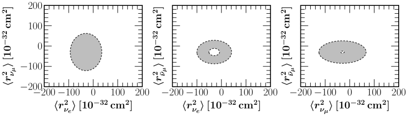
Figure 15: Sensitivity in the $(\langle r_{\nu_{\alpha}}^{2}\rangle,\langle r_{\nu_{\beta}}^{2}\rangle)$ parameter space at 90% C.L. from the analysis of the COHERENT data. Taken from Ref. [78].

III.5 The existence of the sterile neutrinos

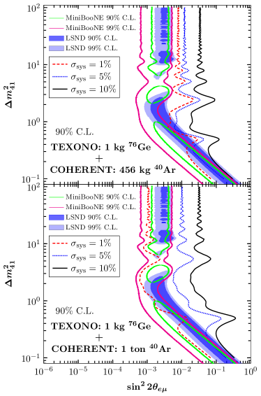
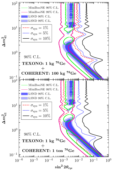
Figure 16: Exclusion curves at 90% C.L. in the ($\Delta m^{2}_{41}$–$\rm{sin}^{2}2\theta_{e\mu}$) parameter plane from a combined analysis of COHERENT and TEXONO experiments. The results are compared to existing constraints from MiniBooNE and LSND. Figure reproduced from Ref. [24] with the permission of the American Physical Society and with updated results from MiniBooNE [142].

The three-neutrino paradigm has been put in rather solid grounds from the interpretation of solar and atmospheric oscillation data. On the other hand, controversial anomalies such as those coming from recent reactor data as well as existing anomalies implied by the LSND and MiniBooNE experiments inspired a reach phenomenology beyond the three-neutrino oscillation picture, based on the existence of a fourth sterile neutrino state with eV-scale mass ($m_{1,2,3}\ll m_{4}$) and tiny mixing angles. To accommodate sterile neutrinos the lepton mixing matrix is minimally extended so that the flavor eigenstates $\nu_{\alpha}$, ($\alpha=e,\mu,\tau,s,\cdots$) are related to the mass eigenstates $\nu_{i}$ ($i=1,2,3,4,\cdots$) by the unitary transformation $\nu_{\alpha}=\sum_{i}U_{\alpha i}\nu_{i}$. Then, for the short-baseline CE$\nu$NS experiments the survival probability of an active neutrino at a distance $L$ is written [26]

$$P_{\alpha\rightarrow e,\mu,\tau}=1-4\left|U_{\alpha 4}\right|^{2}\left(1-\sum_{\beta=e,\mu,\tau}\left|U_{\beta 4}\right|^{2}\right)\rm{sin}^{2}\left(\Delta\right)\,,$$ (63)

with the abbreviation $\Delta\equiv\Delta m^{2}L/4E_{\nu}$ and the mass splittings under the approximation $\Delta m^{2}_{41}\approx\Delta m^{2}_{42}\approx\Delta m^{2}_{43}\equiv\Delta m^{2}$. At this point it should be stressed that neutrino-nucleus scattering experiments are favorable facilities to probe sterile neutrinos being complementary to dedicated experiments such as MINOS/MINOS+ [143], MiniBooNE [142], Daya-Bay [144], Juno [145] and NEOS [146]. Indeed, due to the purely neutral-current character of the CE$\nu$NS process it is not necessary to disentangle between active-sterile neutrino mixing [147].

The possibility of investigating sterile neutrinos in the simplest (3+1) scheme through the CE$\nu$NS process was examined for the first time in Ref. [148], relying on an SNS source. A combined sterile neutrino analysis was performed in Ref. [24] highlighting the complementarity between accelerator and reactor neutrino sources, by focusing on COHERENT and TEXONO experiments respectively (see Fig. 16). Moreover, a detailed study of various reactor-based CE$\nu$NS proposals has been carried out in Ref. [25], showing how such future measurements can be exploited to solve the reactor antineutrino anomaly. After the first observation of CE$\nu$NS by the COHERENT experiment, Ref. [21] reported the first constraints under the assumption of a universal new mixing angle, extracting the conclusion that the current sensitivity is rather poor. By exploiting timing data the potential of a future measurement at the next generation of COHERENT with a 100 kg CsI detector has been demonstrated in Ref. [26], concluding that the prospects of probing the exclusion regions in the ($\Delta m^{2}_{41}$–$\rm{sin}^{2}2\theta_{e\mu}$) plane from the latest MiniBooNE [142] and LSND [149] are promising. Finally, focusing at CONUS in Ref. [150] it was shown that the complementarity between terrestrial-cosmological experiments may resolve the tension raised by astrophysical observations regarding the existence of sterile neutrinos.

III.6 Summary of constraints

Emphasis has been put on the physics beyond the SM by devoting a great part to the past and current research efforts and by concentrating on the various channels contributing to CE$\nu$NS processes and their interpretation. Through a $\chi^{2}$ sensitivity analysis based on the recoil or timing spectra of the COHERENT data, the current limits are listed at 90% C.L. in Table 2. For a given parameter set $\mathcal{S}$, the best fit is found through the minimum value $\chi^{2}_{\text{min}}(\mathcal{S})$. The limits involve electroweak (weak-mixing angle), nuclear (nuclear radius), and physics beyond the SM (NSIs and EM neutrino properties). Significant improvements are expected through a more accurate determination of the QF and from a better control of the systematic uncertainties. The reported constraints on electroweak and NSIs have been extracted with various analysis methods, i.e. by combining existing APV measurements or global oscillation constraints with the recent COHERENT data, emphasizing the complementarity of CE$\nu$NS data in the low energy regime.

Parameter	dataset	Reference	Limit (90% C.L.)
$\rm{sin}^{2}\theta_{W}$ a	COHERENT + APV	[101]	$0.239^{+0.006}_{-0.007}$
$R_{n}$			$5.42^{+0.50}_{-0.50}$
$\epsilon_{ee}^{uV}$	COHERENT + oscillation	[151]	0.028 – 0.60
$\epsilon_{ee}^{dV}$			0.030 – 0.55
$\epsilon_{\mu\mu}^{uV}$			-0.088 – 0.37
$\epsilon_{\mu\mu}^{dV}$			-0.075 – 0.33
$\epsilon_{ee}^{uT}$	COHERENT (recoil)	[21]	-0.013 – 0.013
$\epsilon_{ee}^{dT}$			-0.011 – 0.011
$\epsilon_{\mu\mu}^{uT}$			-0.013 – 0.013
$\epsilon_{\mu\mu}^{dT}$			-0.011 – 0.011
$\mu_{\nu}$	COHERENT (recoil)	[21]	$<43$
$\mu_{\nu_{e}}$			$<52$
$\mu_{\nu_{\mu}}$			$<46$
$\langle r^{2}_{\nu_{e}}\rangle$	COHERENT (timing and recoil)	[152]	-63 – 12
$\langle r^{2}_{\nu_{\mu}}\rangle$			-7 – 9
$\langle r^{2}_{\nu_{e\mu}}\rangle$			$<22$
$\langle r^{2}_{\nu_{e\tau}}\rangle$			$<37$
$\langle r^{2}_{\nu_{\mu\tau}}\rangle$			$<26$
a The limit is shown at 1$\sigma$.

Table 2: Constraints on electroweak, nuclear and new physics parameters at 90% C.L. after the first CE$\nu$NS measurement by the COHERENT experiment. The limits are presented in units of: fm for the nuclear rms radius, $10^{-10}\,\mu_{B}$ for the neutrino magnetic moment and $10^{-32}\,\mathrm{cm^{2}}$ for the neutrino charge radius.

IV Connection of CE$\nu$NS with Dark Matter, cLFV processes and astrophysics

Neutrino-nucleus scattering is one of the dominant processes taking place in SN environment and thus the emitted neutrinos can be an extremely useful tool for deep sky investigations. Moreover, SN constitute an ideal source for flavor physics applications since all flavors are involved. Going beyond the SM, potential FCNC under stellar conditions can modify the percentage of the neutrino flavors in the interior of massive stars [58]. The latter, may drastically affect a plethora of other processes governing the explosive-stellar nucleosynthesis [153], causing significant alteration of the evolution phenomena [114, 154]. If large enough, the modified neutrino energy-densities arriving at the terrestrial SN-neutrino detectors can be tested at CE$\nu$NS experiments [155]. It should be stressed that a SN neutrino burst can be well detected by the current technology DM detectors.

Direct Dark Matter detection experiments are expected to be sensitive to astrophysical neutrinos from the Sun, the Atmosphere and from core-collapse SN (e.g. diffuse supernova background, DSNB) [156, 157]. The neutrino-floor [158], being an irreducible background determines the criteria for using the appropriate detector material, threshold, mass, etc. Figure 17 illustrates the differential and integrated event rate of CE$\nu$NS expected at a ton-scale DM detector, calculated in the framewrok of the DSM assuming only SM interactions. Future precision measurements at such rare-event facilities may become sensitive to nuclear structure effects which in principle can be explored by experiments looking for CE$\nu$NS. Therefore precise information on the nuclear form factors becomes very relevant for DM detectors especially for those involving multi-ton mass scale [35]. For example, alterations are expected at high recoil energies of neutrino-induced interactions at direct DM detection searches [39] which on the other hand may be limited by the current uncertainties of the Atmospheric and DSNB neutrinos. Models involving light mediators are well testable at CE$\nu$NS searches and may offer a key solution to LMA-Dark [159, 151] as well as implications to DM searches [28, 133] and to the neutrino floor [40]. In the same spirit, combined analyses of oscillation and CE$\nu$NS data [18, 15] concluded that the LMA-D solution is excluded at $3.1\sigma$ ($3.6\sigma$) for NSI with up (down) quarks. Finally, it has been recently pointed out that potential DM-induced signatures from dark photon decay could be also detectable at CE$\nu$NS experiments, explaining an excess in the timing distribution of the COHERENT signal [44].

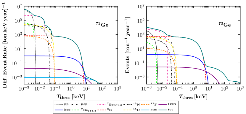
Figure 17: Differential event rate (left) and total number of events above threshold (right) expected due to CE$\nu$NS from solar, Atmospheric and DSNB neutrinos at a Germanium detector. Figure adapted from Ref. [39] under the terms of the Creative Commons Attribution 4.0 International license.

In the case of cLFV processes of $\mu\to e$ transitions, especially coherent $\mu^{-}\to e^{-}$ conversion in the field of nuclei has attracted much interest in the context of new physics mechanisms discussed in this article [160]. For example, $\mu\to e$ conversion has been studied in the context of the inverse seesaw [109] and new $Z^{\prime}$ mediators [161]. It is given by

$$\mu^{-}+(A,Z)\rightarrow e^{-}+(A,Z)\,,$$ (64)

which might have close relations to the process given in Eq.(36) in the neutral sector. When the final nuclear state coincides with the ground state, this process could be a coherent channel, which in fact dominates by its enhancement by a factor of the square of the number of nucleons in nuclei. The cLFV processes are known to be highly suppressed in the SM even with lepton mixing due to the small neutrino masses, down to $\mathcal{O}(10^{-54})$ [162]. However, many theoretical models involving NSI predict sizable rates which the future experiments could reach [163]. The future experiments aiming to search for $\mu^{-}\to e^{-}$ conversion are under preparation at J-PARC, Japan (COMET) [164] and Fermilab, in the USA (Mu2e) [165]. They expect to measure a characteristic peak of outgoing electrons (at energy $E_{e}\approx m_{\mu}$) emitted from muonic atoms in a target. These experiments are aiming at sensitivities of the order of $\mathcal{O}(10^{-17})$ to $\mathcal{O}(10^{-18})$ , which is a factor of 10,000 or more improvement over the current experimental limits. Therefore they have excellent potential to establish or rule out the presence of new physics in the near future.

It is important to notice that theoretically the $\mu^{-}\to e^{-}$ branching ratio depends on the nuclear form factor which can be probed from CE$\nu$NS measurements as discussed in Sect III. For the relevant nuclei such as ²⁷Al and ⁴⁸Ti the nuclear form factors at $q\approx m_{\mu}=0.53~{}\mathrm{fm^{-1}}$ have values 0.63 and 0.53 respectively i.e. well far from the approximation of point like nucleus (see Ref. [81] for a detailed discussion). The incoherent channels of $\mu\to e$ conversion can be studied with the matrix elements described in Sect. II (see for example Refs. [166, 82]). Once $\mu^{-}\to e^{-}$ conversion is observed, it holds significant potential for constraining the parameters of the NSI Lagrangian of the lepton-nucleus interactions [167]. It may shed light on FCNC processes in the leptonic sector [168, 169, 170], and particularly on the existence of the charged-lepton mixing which is analogous to neutrino oscillations at short baseline experiments.

V Summary and conclusions

In this review article, we made an attempt to summarize the main research efforts devoted to the conventional and exotic neutrino-nucleus interactions, in the recent years. The standard process of neutral-current neutrino-nucleus scattering, mediated by the neutral $Z$-boson presents two channels: the elastic and inelastic scattering of neutrinos (and anti-neutrinos) off a nuclear isotope $(A,Z)$, with $A$ nucleons and $Z$ protons. In the elastic process, the initial and final states of the target nucleus are the same and the detectable signal is an energy recoil, whereas in the case of the inelastic channel the final nucleus is an excited state with the signal being a de-excitation product (gammas). We have mainly concentrated on beyond the SM neutrino-nucleus interactions, and especially on the prospects of extracting new physics from the operating prominent rare-event detectors looking for the coherent elastic neutrino-nucleus scattering. Such channels may involve lepton LFV in neutral-currents. This is motivated by the recent measurements of CE$\nu$NS events at the COHERENT experiment, the analysis and interpretation of which may imply the necessity of including non-standard neutrino-nucleus interactions. Towards this end, we discussed the impact of non-standard interactions and novel $Z^{\prime}$ or $\phi$ mediators to the CE$\nu$NS event rates providing an estimation of the attainable sensitivities at current and future experiments. With regards to neutrino oscillations constraints on NSIs from neutral current interactions at CE$\nu$NS experiments are complementary since the former are only to sensitive to differences between the diagonal terms. It is furthermore expected that the next generation of the currently operating experiments like the COHERENT, TEXONO, MINER, CONUS, RED100, vGEN, Ricochet, NUCLEUS etc., will be of benefit to unravel open issues of the leptonic sector. The studies covered in this review article have evident connection with neutrino astronomy, SN physics, direct DM detection and cLFV processes. To understand these new interactions the proton and neutron weak nuclear form factors play key roles. This opens up the necessity of measuring the neutron nuclear form factors by appropriately designed and appreciably sensitive experiments such as those looking for CE$\nu$NS processes.

Appendix A

A.1 Multipole operators

The Donnelly-Walecka multipole decomposition method yields a set of eight linearly independent irreducible tensor operators which are typically expressed in terms of the Spherical Bessel functions, $j_{l}$, and combined with the Spherical Harmonics, $Y^{L}_{M}$, or the vector Spherical Harmonics, ${\bf Y}^{(L,1)J}_{M}$ [171]

$$M^{J}_{M}(\kappa{\bf r})\,=\,\delta_{LJ}j_{L}(\kappa r)Y^{L}_{M}(\hat{r}),$$ (65)

$${\bf M}_{M}^{(L1)J}(\kappa{\bf r})\,=\,j_{L}(\kappa r){{\bf Y}}_{M}^{(L1)J}(\hat{r})\,,$$ (66)

with

$${\bf Y}^{(L,1)J}_{M}(\hat{r})\,=\,\sum_{M_{L},\lambda}\langle LM_{L}1\lambda|JM\rangle Y^{L}_{M_{L}}(\hat{r})\mathbf{e}_{\lambda}\,.$$ (67)

As a consequence of the V-A structure of electroweak interactions

$$\hat{\mathcal{J}}_{\mu}={\hat{J}}_{\mu}-{\hat{J}}^{5}_{\mu}=({\hat{\rho}},\hat{\bf J})-({\hat{\rho}}^{5},\hat{\bf J}^{5})\,,$$ (68)

four operators are associated to the vector component $\hat{J}_{\lambda}=(\hat{\rho},\bf{\hat{J}})$ and four to the axial-vector component $\hat{J}_{\lambda}^{5}=(\hat{\rho}^{5},\bf{\hat{J}^{5}})$ of the hadronic current

$$\hat{\mathcal{M}}_{JM}(\kappa) = \hat{M}_{JM}^{coul}-\hat{M}_{JM}^{coul5}=\int d{\bf r}M^{J}_{M}(\kappa{\bf r})\hat{\mathcal{J}}_{0}({\bf r}),$$ (69)

$$\hat{\mathcal{L}}_{JM}(\kappa) = \hat{L}_{JM}-\hat{L}_{JM}^{5}=i\int d{\bf r}\left(\frac{1}{\kappa}\boldsymbol{\nabla}M^{J}_{M}(\kappa{\bf r})\right)\cdot\hat{\mathcal{J}}({\bf r}),$$ (70)

$$\hat{\mathcal{T}}_{JM}^{el}(\kappa) = \hat{T}_{JM}^{el}-\hat{T}_{JM}^{el5}=\int d{\bf r}\left(\frac{1}{q}\boldsymbol{\nabla}\times{\bf M}^{JJ}_{M}(\kappa{\bf r})\right)\cdot\hat{\mathcal{J}}({\bf r}),$$ (71)

$$\hat{\mathcal{T}}_{JM}^{mag}(\kappa) = \hat{T}_{JM}^{mag}-\hat{T}_{JM}^{mag5}=\int d{\bf r}{\bf M}^{JJ}_{M}(\kappa{\bf r})\cdot\hat{\mathcal{J}}({\bf r})\,,$$ (72)

where $\kappa=|\mathbf{q}|$ denotes the 3-momentum transfer. Note that, the vector component yields the Coulomb $M_{JM}^{coul}$, longitudinal $L_{JM}$, transverse electric $T^{el}_{JM}$ (normal parity $\pi=(-)^{J}$) and transverse magnetic $T^{mag}_{JM}$ (abnormal parity $\pi=(-)^{J+1}$), while regarding the axial-vector component $M_{JM}^{coul5}$, $L_{JM}^{5}$, $T^{el5}_{JM}$ have abnormal parity and $T^{mag5}_{JM}$ has normal parity. The matrix elements of the above operators involve momentum dependence of the nucleon form factors $F_{X}(Q^{2})$, $X=1,A,P$ and $\mu^{V}(Q^{2})$

$$\hat{M}_{JM}^{coul}(\kappa{\bf r}) = F_{1}^{V}(Q^{2})M^{J}_{M}(\kappa{\bf r})\,,$$ (73)

$$\hat{L}_{JM}(\kappa{\bf r}) = \frac{q_{0}}{\kappa}\hat{M}_{JM}^{coul}(\kappa{\bf r})\,,$$ (74)

$$\hat{T}_{JM}^{el}(\kappa{\bf r}) = \frac{\kappa}{m_{N}}\left[F_{1}^{V}(Q^{2}){\Delta^{\prime}}^{J}_{M}(\kappa{\bf r})+\frac{1}{2}\mu^{V}(Q^{2}){\Sigma}^{J}_{M}(\kappa{\bf r})\right]\,,$$ (75)

$$i\hat{T}_{JM}^{mag}(\kappa{\bf r}) = \frac{\kappa}{m_{N}}\left[F_{1}^{V}(Q^{2})\Delta^{J}_{M}(\kappa{\bf r})-\frac{1}{2}\mu^{V}(Q^{2}){\Sigma^{\prime}}^{J}_{M}(\kappa{\bf r})\right]\,,$$ (76)

$$i\hat{M}_{JM}^{5}(\kappa{\bf r}) = \frac{\kappa}{m_{N}}\Biggr{[}F_{A}(Q^{2})\Omega^{J}_{M}(\kappa{\bf r})+\frac{1}{2}\left(F_{A}(Q^{2})+q_{0}F_{P}(Q^{2})\right){\Sigma^{\prime\prime}}^{J}_{M}(\kappa{\bf r})\Biggl{]}\,,$$ (77)

$$-i\hat{L}_{JM}^{5}(\kappa{\bf r}) = \left[F_{A}(Q^{2})-\frac{\kappa^{2}}{2m_{N}}F_{P}(Q^{2})\right]{\Sigma^{\prime\prime}}^{J}_{M}(\kappa{\bf r})\,,$$ (78)

$$-i\hat{T}_{JM}^{el5}(\kappa{\bf r}) = F_{A}(Q^{2}){\Sigma^{\prime}}^{J}_{M}(\kappa{\bf r})\,,$$ (79)

$$\hat{T}_{JM}^{mag5}(\kappa{\bf r}) = F_{A}(Q^{2}){\Sigma}^{J}_{M}(\kappa{\bf r})\,.$$ (80)

It becomes evident that only seven are linearly independent

$$T_{1}^{JM}\, \equiv \,M^{J}_{M}(\kappa{\bf r})\,=\,\delta_{LJ}\,j_{L}(\kappa{\bf r})Y^{L}_{M}(\hat{r}),$$ (81)

$$T_{2}^{JM}\, \equiv \,{\Sigma}^{J}_{M}(\kappa{\bf r})\,=\,{{\bf M}}^{JJ}_{M}\cdot\mbox{\boldmath$\sigma$},$$ (82)

$$T_{3}^{JM}\, \equiv \,{\Sigma^{\prime}}^{J}_{M}(\kappa{\bf r})\,=\,-i\left[\frac{1}{\kappa}\boldsymbol{\nabla}\times{{\bf M}}^{JJ}_{M}(\kappa{\bf r})\right]\cdot\mbox{\boldmath$\sigma$},$$ (83)

$$T_{4}^{JM}\, \equiv \,{\Sigma^{\prime\prime}}^{J}_{M}(\kappa{\bf r})\,=\,\Big{[}\frac{1}{\kappa}\boldsymbol{\nabla}M^{J}_{M}(\kappa{\bf r})\Big{]}\cdot\mbox{\boldmath$\sigma$},$$ (84)

$$T_{5}^{JM}\, \equiv \,{\Delta}^{J}_{M}(\kappa{\bf r})\,=\,{{\bf M}}^{JJ}_{M}(\kappa{\bf r})\cdot\frac{1}{\kappa}\boldsymbol{\nabla},$$ (85)

$$T_{6}^{JM}\, \equiv \,{\Delta^{\prime}}^{J}_{M}(\kappa{\bf r})\,=\,-i\Big{[}\frac{1}{\kappa}\boldsymbol{\nabla}\times{{\bf M}}^{JJ}_{M}(\kappa{\bf r})\Big{]}\cdot\frac{1}{\kappa}\boldsymbol{\nabla},$$ (86)

$$T_{7}^{JM}\, \equiv \,\Omega^{J}_{M}(\kappa{\bf r})\,=\,M^{J}_{M}(\kappa{\bf r})\mbox{\boldmath$\sigma$}\cdot\frac{1}{\kappa}\boldsymbol{\nabla}\,.$$ (87)

In the proton-neutron representation, $T_{i}^{JM}(\kappa{\bf r})$, $i=1,2,\cdots,7$ can be written in closed form [65]

$$\langle j_{1}||T_{i}^{J}||j_{2}\rangle=e^{-y}y^{\beta/2}\sum_{\mu=0}^{n_{max}}\mathcal{P}_{\mu}^{i,\,J}y^{\mu},\qquad i=1,\cdots,7.$$ (88)

A.2 Coefficients for calculating the charge density distribution and form factors in the context of FOP

The coefficients $\theta_{\lambda}$ of the polynomial $\Phi\left(|\mathbf{q}|\,b,Z\right)$ are evaluated, as

$$\theta_{\lambda}=\frac{\sqrt{\pi}}{4^{\lambda}}\sum_{\begin{subarray}{c}(n,l)j\\ (2n+l>\lambda)\end{subarray}}^{N_{\mathrm{max}}}\sum_{m=s}^{2n}\frac{(2j+1)n!C_{nl}^{m}\Lambda_{\lambda}(m+l,0)(l+m)!}{2\Gamma(n+l+\frac{3}{2})}\,.$$ (89)

In the latter expression, $\Gamma(x)$ denotes the Gamma function while the definition of the index $s$ is

$$s=\begin{cases}0,&\text{if }\lambda-l\leq 0\\ \lambda-l&\text{if }\lambda-l>0\end{cases}\,,$$ (90)

and

$$\Lambda_{k}(n,l)=\frac{(-)^{k}}{k!}\left(\begin{array}[]{c}{n+l+1/2}\\ {n-k}\end{array}\right),\quad C_{nl}^{m}=\sum_{k=0}^{m}\Lambda_{m-k}(n,l)\Lambda_{k}(n,l)\,.$$ (91)

The corresponding coefficients $f_{\lambda}$ are written as

$$f_{\lambda}=\sum_{(n,l)j}\frac{\pi^{1/2}(2j+1)n!\,C_{nl}^{\lambda-l}}{2\Gamma\left(n+l+\frac{3}{2}\right)}\,.$$ (92)

As a concrete example the coefficients $\theta_{\lambda}$ and $f_{\lambda}$ for even-even nuclei up to ⁵⁰Sn are listed in Table 3.

$Z$ ($N$)	$(nl)j$	$\lambda=0$		$\lambda=1$		$\lambda=2$		$\lambda=3$		$\lambda=4$
2	$0s_{1/2}$	$2$	$(~{}2)$
6	$0p_{3/2}$	$2$	$(~{}6)$	$\frac{8}{3}$	$(~{}-\frac{2}{3})$
8	$0p_{1/2}$	$2$	$(~{}8)$	$4$	$(~{}-1)$
14	$0d_{5/2}$	$2$	$(14)$	$4$	$(~{}-3)$	$\frac{8}{5}$	$(\frac{1}{10})$
18	$0d_{3/2}$	$2$	$(18)$	$4$	$(-\frac{13}{3})$	$\frac{8}{3}$	$(~{}\frac{1}{6})$
20	$1s_{1/2}$	$5$	$(20)$	$0$	$(~{}-5)$	$4$	$(~{}\frac{1}{4})$
22	$1p_{1/2}$	$5$	$(22)$	$\frac{10}{3}$	$(~{}-6)$	$\frac{4}{3}$	$(\frac{13}{3})$	$\frac{8}{15}$	$(-\frac{1}{120})$
30	$0f_{7/2}$	$5$	$(30)$	$\frac{10}{3}$	$(-10)$	$\frac{4}{3}$	$(~{}\frac{5}{6})$	$\frac{8}{7}$	$(~{}-\frac{1}{56})$
34	$1p_{3/2}$	$5$	$(34)$	$10$	$(-12)$	$-4$	$(~{}\frac{6}{5})$	$\frac{232}{105}$	$(-\frac{29}{840})$
40	$0f_{5/2}$	$5$	$(40)$	$10$	$(-15)$	$-4$	$(~{}\frac{3}{2})$	$\frac{8}{3}$	$(~{}-\frac{1}{24})$
50	$0h_{9/2}$	$5$	$(50)$	$10$	$(-\frac{65}{3})$	$-4$	$(~{}\frac{5}{2})$	$\frac{8}{3}$	$(~{}-\frac{5}{56})$	$\frac{32}{189}$	$(\frac{1}{1512})$

Table 3: Calculated coefficients $f_{\lambda}$ $(\theta_{\lambda})$ for the determination of the proton/neutron density distributions (nuclear form factors). Table adapted from Ref. [61] under the terms of the Creative Commons Attribution 4.0 International license.