Confinement/deconfinement phase transition and dual Meissner effect
in SU(3) Yang-Mills theory

Abstract

We investigate the confinement-deconfinement phase transition at finite temperature of the $SU(3)$ Yang-Mills theory on the lattice from a viewpoint of the dual superconductor picture based on the novel reformulation of the Yang-Mills theory. In particular, we compare the conventional Abelian dual superconductor picture with the non-Abelian dual superconductor picture proposed in our previous works as the mechanism of quark confinement in the $SU(3)$ Yang-Mills theory. For the $SU(3)$ Yang-Mills theory, the reformulation allows two possible options called maximal and minimal. The maximal option corresponds to the manifestly gauge-invariant extension of the Abelian projection scheme, while the minimal option is really new to give the non-Abelian dual superconductor picture due to non-Abelian magnetic monopoles. Keeping these differences in mind, we present the numerical evidences that the confinement/deconfinement phase transition is caused by appearance/disappearance of the dual Meissner effects. First, we measure the Polyakov loop average at various temperatures to determine the critical temperature separating the low-temperature confined phase and the high-temperature deconfined phase. Second, we measure the static quark-antiquark potential at various temperatures. Third, we measure the chromoelectric and chromomagnetic flux created by a pair of quark and antiquark at temperatures below and above the critical temperature. We observe no more squeezing of the chromoelectric flux tube at high-temperatures above the critical temperature. Finally, we measure the associated magnetic–monopole current induced around the chromo-flux tube and observe that the confinement/deconfinement phase transition is associated with the appearance/disappearance of the induced magnetic–monopole current, respectively. We confirm that these results are also obtained by the restricted field alone in both options, indicating the restricted field dominance in quark confinement at finite temperature.

year number number identifier

I Introduction

The dual superconductivity is one of the most promising mechanisms for quark confinement dualsuper . To establish the dual superconductor picture, we must show that magnetic monopoles play a dominant role in quark confinement. For this purpose, we have constructed a new formulation KMS05 of the $SU(N)$ Yang-Mills theory on the continuum space-time which enables us to define the gauge-invariant magnetic monopoles in the gauge-independent way. Subsequently, we have implemented the new formulation to the $SU(N)$ Yang-Mills theory on the lattice KKMSSI06 ; KSSMKI08 ; SKS10 , which enables us to perform the numerical simulations to obtain non-perturbative results. The new reformulation is feasible for decomposing the gauge field into the two pieces, i.e., the restricted field and the remaining one in the gauge covariant way so that the restricted field is identified with the dominant mode for quark confinement in the gauge independent way. See KKSS15 for a review.

The conventional method called the Abelian projection tHooft81 allows us to extract specific magnetic monopoles called Abelian magnetic monopoles in the pure Yang-Mills theory without matter fields, which are however possible only in special Abelian gauges such as the maximal Abelian (MA) gauge KLSW87 and the Laplacian Abelian gauge. In fact, the Abelian projection is a kind of gauge fixing to explicitly break the gauge symmetry, which also breaks the color symmetry (global symmetry). Therefore, the Abelian magnetic monopoles are not gauge-independent objects. This fact casts a doubt on the validity of the results obtained under the Abelian projection.

The new formulation can overcome the criticism raised for the Abelian projection method to extract magnetic monopoles in the pure Yang-Mills theory without matter fields. The new formulation of the $SU(3)$ Yang-Mills theory has two possible options for choosing the fundamental field variables which we call the minimal and maximal options. The respective option is discriminated by a maximal stability subgroup $\tilde{H}$, a subgroup of the gauge group $G$.

In the minimal option, the maximal stability group is the non-Abelian group $\tilde{H}=U(2)\cong SU(2)\times U(1)$ and the restricted field is used to extract non-Abelian magnetic monopoles yielding non-Abelian dual superconductivity. In the preceding works, indeed, we have provided numerical evidences of the non-Abelian dual superconductivity using the minimal option for the $SU(3)$ Yang-Mills theory on a lattice. The minimal option is suggested from the non-Abelian Stokes theorem Kondo08 ; KS08 for the Wilson loop operator in the fundamental representation. We have found that both the restricted field variable and the extracted non-Abelian magnetic monopole dominantly reproduce the string tension in the linear potential of the $SU(3)$ Yang-Mills theory KSSK11 . In this way we have demonstrated the gauge-independent restricted field dominance (corresponding to the conventional Abelian dominance): the string tension $\sigma_{V}$ calculated from the restricted field reproduces the string tension $\sigma_{full}$ of the original Yang-Mills field: $\sigma_{V}/\sigma_{full}=93\pm 16\%$. Moreover, we have also demonstrated the gauge-independent non-Abelian magnetic monopole dominance: the string tension $\sigma_{V}$ was reproduced by $\sigma_{mon}$ calculated from the (non-Abelian) magnetic monopole part extracted from the restricted field: $\sigma_{mon}/\sigma_{V}=94\pm 9\%$, see KSSMKI08 ; lattice2008 ; lattice2009 ; lattice2010 ; KSSK11 .

The dual superconductivity has been established by demonstrating the existence of chromoelectric flux connecting a quark and antiquark and the associated magnetic-monopole current induced around the flux tube KSSK11 where both the chromoelectric flux and the magnetic-monopole current are gauge-invariant objects. Moreover, the investigation of the chromoelectric flux tube leads to the surprising conclusion that the vacuum of the $SU(3)$ Yang-Mills vacuum is the type I dual superconductor, which is a novel feature obtained by the numerical simulations SKKS13 . This is sharp contrast to the proceeding studies: the border of type I and type II or of week type I flusx:AP . In the $SU(3)$ case, there are many works on chromo flux by using Wilson line/loop operator, see e.g., Cardaci2011 ; Cardso ; CCP12 ; CCCP14 .

These results should be compared with another option called the maximal option which was first constructed by Cho SUN-decomp1 and Faddeev and Niemi SUN-decomp2 by extending the Cho-Duan-Ge-Faddeev-Niemi (CDGFN) decomposition for the $SU(2)$ case CFNS-C . The maximal stability group in the maximal option of $SU(3)$ is an Abelian group $\tilde{H}=U(1)\times U(1)$, the maximal torus subgroup of $SU(3)$. Therefore, the restricted field in the maximal option involves only the Abelian magnetic monopole, which is indeed detected on the lattice lattce2007 ; CCLL14 . The maximal option in the new formulation gives a gauge invariant extension of the Abelian projection in the maximal Abelian (MA) gauge GIS12 ; SS14 .

The similar results are also obtained for $SU(2)$ Yang-Mills theory on the lattice IKKMSS06 ; SKKMSI07 ; lattice2009k ; Cea1995 ; Cea2012a14 . The restricted field corresponding to the stability group $\tilde{H}=U(1)$ of $SU(2)$ reproduces the dual Meissner effect KKS14 ; NKSSK2018 . For $SU(2)$, there is a unique option which is regarded as a gauge-invariant version of the Abelian projection in the MA gauge SY90 ; SS94 ; SNW94 .

Furthermore, the dual superconductivity for the Wilson loop in higher representations is investigated by using the extension of the new formulation of the $SU(N)$ Yang-Mills theory on the lattice. The restricted field reproduces the string tension in the linear potential of the $SU(3)$ Yang-Mills theory for the Wilson loops in higher representations MSKK2019 .

The purpose of this paper is to investigate the confinement/deconfinement phase transition at finite temperature of the $SU(3)$ Yang-Mills theory from a viewpoint of the dual superconductor picture, as an investigation subsequent to quark confinement due to dual superconductivity in the $SU(3)$ Yang-Mills theory at zero temperature, see lattice2012 ; lattice2013 ; lattice2014 ; lattice2015 ; lattice2016 ; SCGT15 ; confinementX ; confinement2018 for preliminary results. In particular, we compare the conventional Abelian dual superconductor picture with the non-Abelian dual superconductor picture proposed as the mechanism of quark confinement in the $SU(3)$ Yang-Mills theory in our previous works based on the novel reformulation of the Yang-Mills theory. We examine the dual Meissner effect at finite temperature by measuring the distribution of the chromoelectric field strength (or chromo flux) generated from a static quark-antiquark pair and the associated magnetic-monopole current induced around it. We present the numerical evidences for them at finite temperature by using the gauge link decomposition for extracting the magnetic monopole in the gauge invariant way. In particular, we discuss the role of magnetic monopoles in confinement/deconfinement phase transition. We focus on whether there are distinctions for the physics of quark confinement between the maximal and minimal options in the new reformulation of the $SU(3)$ Yang-Mills theory.

This paper is organized as follows. In section II, we review the new formulations of the $SU(3)$ Yang-Mills theory on the lattice to see the differences between the minimal and maximal options. In section III, we give the results of the numerical simulations on the lattice. First, we measure the Polyakov loop average at various temperatures to determine the critical temperature $T_{c}$ separating the low-temperature confined phase and the high-temperature deconfined phase. We also measure the correlation functions of the Polyakov loops which are defined for both the original Yang-Mills gauge field and the restricted field to examine the restricted field dominance in the Polyakov loop average at finite temperature. Second, we measure the string tension for the restricted field of both minimal and maximal option in comparison with the string tension for the original gauge field. Third, we investigate the dual Meissner effect by measuring the distribution of the chromoelectric flux and chromomagnetic flux created by a pair of static quark and antiquark at finite temperature below and above the critical temperature to investigate its relevance to the phase transition. We observe no more squeezing of the chromoelectric flux tube in the high-temperature deconfinement phase above the critical temperature $T_{c}$. Finally, we measure the associated magnetic–monopole current induced around the chromo-flux tube and observe that the confinement/deconfinement phase transition is associated with the appearance/disappearance of the induced magnetic–monopole current, respectively. We observe that these results are also obtained by the restricted field alone, confirming the restricted field dominance at finite temperature. These results are the numerical evidences that the confinement/deconfinement phase transition is caused by appearance/disappearance of the non-Abelian dual superconductivity. The final section is devoted to conclusion and discussion.

II New formulation of lattice gauge theory

II.1 Gauge link decompositions

We introduce a new formulation of the lattice Yang-Mills theory, which enables one to extract the dominant mode for quark confinement in the $SU(N)$ Yang-Mills theory KKMSSI06 ; KSSMKI08 ; SKS10 . We decompose the gauge link variable $U_{x,\mu}$ into the product of the two variables $V_{x,\mu}$ and $X_{x,\mu}$:

$$U_{x,\mu}=X_{x,\mu}V_{x,\mu}\in G=SU(N),$$

in such a way that the new variable $V_{x,\mu}$ is transformed by the full $SU(3)$ gauge transformation $\Omega_{x}$ as the gauge link variable $U_{x,\mu}$, while $X_{x,\mu}$ transforms as the site variable:

$$U_{x,\mu} \longrightarrow U_{x,\nu}^{\prime}=\Omega_{x}U_{x,\mu}\Omega_{x+\mu}^{{\dagger}},$$ (1a)

$$V_{x,\mu} \longrightarrow V_{x,\nu}^{\prime}=\Omega_{x}V_{x,\mu}\Omega_{x+\mu}^{{\dagger}},$$ (1b)

$$X_{x,\mu} \longrightarrow X_{x,\nu}^{\prime}=\Omega_{x}X_{x,\mu}\Omega_{x}^{{\dagger}}.$$ (1c)

From the physical point of view, $$V_{x,\mu} X_{x,\mu}$$ could be identified with the dominant mode for quark confinement, while is the remaining part.

For the $SU(3)$ Yang-Mills theory, we have two possible options discriminated by the stability subgroup $\tilde{H}$ of the gauge group $G$, which we call the minimal and maximal options.

II.2 Minimal option

The minimal option is obtained for the choice of the stability subgroup $\tilde{H}=U(2)=SU(2)\times U(1)\subset SU(3)$. In the minimal option, we introduce a single color field $\bm{h}_{x}$ taking the value in the Lie algebra as a site variable

$$\bm{h}_{x}=\xi_{x}\frac{\lambda^{8}}{2}\xi_{x}^{{\dagger}}\in Lie[SU(3)/U(2)],$$ (2)

with $\lambda^{8}$ being the last diagonal Gell-Mann matrix and $\xi_{x}$ an $SU(3)$ group element. Then the decomposition is obtained by solving the defining equations:

$$D_{\mu}^{\varepsilon}[V]\bm{h}_{x}:=\frac{1}{\varepsilon}\left[V_{x,\mu}\bm{h}_{x+\mu}-\bm{h}_{x}V_{x,\mu}\right]=0\text{ },$$ (3a)

$$g_{x}:=e^{i2\pi q/3}\exp\left(-ia_{x}^{0}\bm{h}_{x}-i\sum\nolimits_{j=1}^{3}a_{x}^{(j)}\mathbf{u}_{x}^{(j)}\right)\text{ }.$$ (3b)

These defining equations can be solved exactly SKS10 , and the solution is given by

$$V_{x,\mu} =X_{x,\mu}^{{\dagger}}U_{x,\mu}=g_{x}\widehat{L}_{x,\mu}U_{x,\mu},$$ (4a)

$$X_{x,\mu} =\widehat{L}_{x,\mu}^{{\dagger}}\det(\widehat{L}_{x,\mu})^{1/3}g_{x}^{-1},$$ (4b)

$$\widehat{L}_{x,\mu} :=\left(L_{x,\mu}L_{x,\mu}^{{\dagger}}\right)^{-1/2}L_{x,\mu},$$ (4c)

$$\text{\ }L_{x,\mu} :=\frac{5}{3}\mathbf{1}+\frac{2}{\sqrt{3}}(\bm{h}_{x}+U_{x,\mu}\bm{h}_{x+\mu}U_{x,\mu}^{{\dagger}})$$

$$+8\bm{h}_{x}U_{x,\mu}\bm{h}_{x+\mu}U_{x,\mu}^{{\dagger}}.$$ (4d)

Here the variable $$g_{x} U(2) \mathbf{u}_{x}^{(j)} su(2) q g_{x}=\mathbf{1}\,\$$ is the part which is undetermined from Eq.(3a) alone, ’s are -Lie algebra valued, and   is an integer, see SKS10 for the details. In what follows, we chose .

Note that the above defining equations (3a) and (3b) correspond to the continuum version: $D_{\mu}[\bm{V}]\bm{h}(x)=0$ and $\mathrm{tr}(\bm{X}_{\mu}(x)\bm{h}(x))$ $=0$, respectively. By taking the naive continuum limit, indeed, we can reproduce the decomposition in the continuum theory KMS05 :

$$\bm{A}_{\mathbf{\mu}}(x) =\bm{V}_{\mu}(x)+\bm{X}_{\mu}(x),$$ (5a)

$$\bm{X}_{\mu}(x) =ig^{-1}\frac{4}{3}\left[\partial_{\mu}\bm{h}(x),\bm{h}(x)\right]$$

$$+\frac{4}{3}\left[\left[\bm{A}_{\mathbf{\mu}}(x),\bm{h}(x)\right],\bm{h}(x)\right],$$ (5b)

$$\bm{V}_{\mu}(x) =\bm{A}_{\mathbf{\mu}}(x)-ig^{-1}\frac{4}{3}\left[\partial_{\mu}\bm{h}(x),\bm{h}(x)\right]$$

$$-\frac{4}{3}\left[\left[\bm{A}_{\mathbf{\mu}}(x),\bm{h}(x)\right],\bm{h}(x)\right],$$ (5c)

In this way, the decomposition is uniquely determined according to (4), once a set of color fields $\{\bm{h}_{x}\}$ are given. To determine the configuration $\{\bm{h}_{x}\}$ of color fields, we adopt the procedure of minimizing the functional:

$$F_{\text{red}}[\bm{h}_{x}]=\sum_{x,\mu}\mathrm{tr}\left\{(D_{\mu}^{\varepsilon}[U_{x,\mu}]\bm{h}_{x})^{{\dagger}}(D_{\mu}^{\varepsilon}[U_{x,\mu}]\bm{h}_{x})\right\},$$ (6)

which yields the condition to be satisfied for the color field, which we call the reduction condition. Thus we obtain the reformulated Yang-Mills theory written in terms of the new variables ($X_{x,\mu}$,$V_{x,\mu}$), which is equipollent to the original Yang-Mills theory.

			$N_{T}=6$			$N_{T}=8$
$\beta$	$\varepsilon\sqrt{\sigma}$	$\varepsilon$ [fm]	$T$[$\sqrt{\sigma}$]	$T$[MeV]	$T/T_{c}$	$T$[$\sqrt{\sigma}$]	$T$[MeV]	$\ T/T_{c}$
$5.75$	$[0.3544]$	$0.159$	$0.1231$	$54.14$	$0.7483$	$-$	$-$	$-$
$5.8$	$[0.3209]$	$0.144$	$0.5194$	$228.8$	$0.8264$	$0.3896$	$171.4$	$0.6198$
$5.85$	$0.2874(7)$	$0.129$	$0.5799$	$255.2$	$0.9228$	$-$	$-$	$-$
$5.875$	$[0.2763]$	$0.124$	$0.6032$	$265.4$	$0.9598$	$-$	$-$	$-$
$5.9$	$[0.2652]$	$0.119$	$0.6285$	$276.5$	$1.000$	$0.4714$	$207.4$	$0.7500$
$5.925$	$[0.25415]$	$0.114$	$0.6558$	$288.5$	$1.034$	$-$	$-$	$-$
$5.95$	$[0.2431]$	$0.109$	$0.6856$	$301.7$	$1.091$	$-$	$-$	$-$
$6.0$	$0.2209(23)$	$0.0989$	$0.7545$	$332.0$	$1.201$	$0.5659$	$249.0$	$0.9005$
$6.1$	$[0.1905]$	$0.085$	$0.8748$	$385..0$	$1.392$	$0.6561$	$288.7$	$1.044$
$6.2$	$0.1610(9)$	$0.0721$	$1.035$	$455.5$	$1.647$	$0.7763$	$341.6$	$1.235$
$6.3$	$[0.1412]$	$0.0632$	$1.180$	$519.3$	$1.878$	$0.8850$	$389.4$	$1.409$
$6.4$	$0.1214(12)$	$0.0543$	$1.373$	$604.1$	$2.185$	$1.030$	$453.1$	$1.639$
$6.5$	$0.1068(9)$	$0.0478$	$1.561$	$686.6$	$2.483$	$1.171$	$515.1$	$1.862$

Table 1: The summary of temperature $T$ for various $\beta$ and $N_{T}$ for the data set I . The relation between $\beta$ and $\varepsilon\sqrt{\sigma}$ is obtaein from Ref Edward98 , where values of $\varepsilon\sqrt{\sigma}$ in the squared brackets are lack of data but these are obtained by linear interpolation of measured values. The lattice spacing is determined by using the relation $\sigma_{\text{latt}}=\varepsilon^{2}\sigma$ with the physical string tenstion defined by $\sqrt{\sigma}=440MeV$ . The temperuture is obtained by using the relation $1/T=\varepsilon N_{T}$. The critical temperature $T_{c}$ is determined by using the Polyakov loop average and the susceptibility as given in Subsection III.2.

	$\beta=6.2$			$\beta=6.0$
$N_{T}$	$T$[$\sqrt{\sigma}$]	$T$[MeV]	$\ T/T_{c}$	$T$[$\sqrt{\sigma}$]	$T$[MeV]	$\ T/T_{c}$
$24$	$0.2588$	$113.9$	$0.4112$	$0.1886$	$82.89$	$0.3001$
$16$	$0.3882$	$170.8$	$0.6181$	$0.2829$	$124.5$	$0.4502$
$14$	$0.4437$	$195.2$	$0.7061$	$0.3223$	$141.8$	$0.5129$
$12$	$0.5176$	$227.7$	$0.8237$	$0.3772$	$166.0$	$0.6002$
$10$	$0.6211$	$273.3$	$0.9884$	$0.4527$	$199.2$	$0.7204$
$8$	$0.7763$	$341.6$	$1.235$	$0.5659$	$249.0$	$0.9005$
$6$	$1.035$	$455.5$	$1.647$	$0.7545$	$332.0$	$1.201$
$4$	$1.553$	$683.2$	$2.471$	$1.132$	$498.1$	$1.801$

Table 2: The summary of temperature $T$ for various $\beta$ and $N_{T}$ for data set II. The temperatures are determined in the same way as Table 1

II.3 Maximal option

The maximal option is obtained for the choice of the stability subgroup of the maximal torus subgroup of $G$: $\tilde{H}=U(1)\times U(1)\subset SU(3)$. In the maximal option, we introduce two kinds of color fields,

$$\bm{n}_{x}^{(3)} =\xi_{x}\frac{\lambda^{3}}{2}\xi_{x}^{{\dagger}}\in Lie[SU(3)/U(1)\times U(1)],$$ (7a)

$$\bm{n}_{x}^{(8)} =\xi_{x}\frac{\lambda^{8}}{2}\xi_{x}^{{\dagger}}\in Lie[SU(3)/U(2)],$$ (7b)

with $$\lambda^{3} \lambda^{8} \xi SU(3) j=3,8$$, being the two diagonal Gell-Mann matrices and an group element. Then the decomposition is obtained by solving the defining equations ():

$$D_{\mu}^{\varepsilon}[V]\bm{n}_{x}^{(j)}:=\frac{1}{\varepsilon}\left[V_{x,\mu}\bm{n}_{x+\mu}^{(j)}-\bm{n}_{x}^{(j)}V_{x,\mu}\right]=0,$$ (8a)

$$g_{x}:=e^{i2\pi q/3}\exp(-ia_{x}^{3}\bm{n}_{x}^{(3)}-ia_{x}^{(8)}\bm{n}_{x}^{(8)})\text{ .}$$ (8b)

These defining equations can be solved exactly, and the solution is given by

$$V_{x,\mu} =X_{x,\mu}^{{\dagger}}U_{x,\mu},$$ (9a)

$$X_{x,\mu} =\widehat{K}_{x,\mu}^{{\dagger}}\det(\widehat{K}_{x,\mu})^{1/3}g_{x}^{-1},$$ (9b)

$$\widehat{K}_{x,\mu} :=\left(K_{x,\mu}K_{x,\mu}^{{\dagger}}\right)^{-1/2}K_{x,\mu},$$ (9c)

$$K_{x,\mu} :=\mathbf{1}+6(\bm{n}_{x}^{(3)}U_{x,\mu}\bm{n}_{x+\mu}^{(3)}U_{x,\mu}^{{\dagger}})$$

$$+6(\bm{n}_{x}^{(8)}U_{x,\mu}\bm{n}_{x+\mu}^{(8)}U_{x,\mu}^{{\dagger}})\text{ }.$$ (9d)

Here the variable $$g_{x} U(1)\times U(1) q g_{x}=1\,$$ is the part which is undetermined from Eq.(8a) alone, and is an integer, see SKS10 for the details. In what follows, we chose .

Note that the above defining equations (8a) and (8b) correspond to the continuum version: $D_{\mu}[\bm{V}]\bm{n}^{(j)}(x)=0$ and $\mathrm{tr}(\bm{X}_{\mu}(x)\bm{n}^{(j)}(x))$ $=0$, respectively. By taking the naive continuum limit, we can reproduce the decomposition in the continuum theory KMS05 :

$$\bm{A}_{\mu}(x)= \bm{V}_{\mu}(x)+\bm{X}_{\mu}(x),$$ (10a)

$$\bm{X}_{\mu}(x)= ig^{-1}\sum_{j=3,8}[\partial_{\mu}\bm{n}^{(j)}(x),\bm{n}^{(j)}(x)]$$

$$+\sum_{j=3,8}[[\bm{A}_{\mu}(x),\bm{n}^{(j)}(x)],\bm{n}^{(j)}(x)],$$ (10b)

$$\bm{V}_{\mu}(x)= \sum_{j=3,8}(\bm{A}_{\mu}(x)\cdot\bm{n}^{(j)}(x))\bm{n}^{(j)}(x)$$

$$-ig^{-1}\sum_{j=3,8}[\partial_{\mu}\bm{n}^{(j)}(x),\bm{n}^{(j)}(x)].$$ (10c)

To formulate the new theory written in terms of the new variables ($X_{x,\mu}$,$V_{x,\mu}$) which is equipollent to the original Yang-Mills theory, we must determine the configuration of color fields $\{\bm{n}_{x}^{(3)},\bm{n}_{x}^{(8)}\}$. In the maximal option, the color fields $\{\bm{n}_{x}^{(3)},\bm{n}_{x}^{(8)}\}$ are obtained by minimizing the functional:

$$F_{\text{red}}[\bm{n}_{x}^{(3)},\bm{n}_{x}^{(8)}]$$

$$=\sum_{x,\mu}\sum_{j=3,8}\mathrm{tr}\left\{(D_{\mu}^{\varepsilon}[U_{x,\mu}]\bm{n}_{x}^{(j)})^{{\dagger}}(D_{\mu}^{\varepsilon}[U_{x,\mu}]\bm{n}_{x}^{(j)})\right\}.$$ (11)

It should be noticed that the decomposition in the maximal option with the reduction condition obtained from the functional Eq.(11) gives the gauge invariant extension of the Abelian projection in the maximal Abelian (MA) gauge.

III Numerical simulations on the lattice

III.1 Lattice setup

We adopt the standard Wilson action with the inverse gauge coupling constant $\beta=2N_{c}/g^{2}$ ($N_{c}=3)$. We prepare the gauge field configurations (link variables) $\{U_{x,\mu}\}$ on the lattice of size $L^{3}\times N_{T}$ from the two different data sets at finite temperature according to the following setups:

(Data set I) For the fixed spatial size and temporal size $L=24$, $N_{T}=6$, $8$, the temperature varies by changing the coupling $\beta$ in the range $5.8\leq\beta\leq 6.5$ (see Table 1). The lattice spacing $\varepsilon$ and the physical volume vary with temperature $T$.

(Data set II) For the fixed spatial size and coupling constant $L=24$, $\beta=6.0$, $6.2$, the temperature varies by changing the temporal size $N_{T}$ (see Table 2). The lattice spacing $\varepsilon$ and the physical volume are the same for each $\beta$.

Table 1 gives the dictionary of the data set I for obtaining the temperature $T$ for a given lattice size $L^{3}\times N_{T}$ and the coupling constant $\beta$ by making use of the lattice spacing $\varepsilon$. Here the physical units or the lattice spacing is determined on the lattice at zero temperature according to Ref. Edward98 . Table 2 gives the dictionary of the data set II for obtaining the temperature $T$ and the temporal size $N_{T}$  for a given coupling constant $\beta$.

We generate the configurations by using the standard method, i.e., one-sweep update is obtained by applying once the pseudo heat-bath method and twelve-times the over-relaxation method. We thermalize 16000 sweeps with the cold start, and prepare 1000 configurations every 400 sweeps.

We obtain the color field configuration $\{\bm{h}_{x}\}$ for the minimal option by minimizing the functional Eq.(6) for each set of the gauge field configurations $\{U_{x,\mu}\}$,  while we obtain the color field configuration $\{\bm{n}^{(3)}_{x}\}$ and $\{\bm{n}^{(8)}_{x}\}$ for the maximal option by minimizing the functional Eq.(11) for each set of the gauge field configurations $\{U_{x,\mu}\}.$ Then we perform the decomposition of the gauge link variable $U_{x,\mu}=X_{x,\mu}V_{x,\mu}$ by using the formula given in the previous section. In the measurement of the Polyakov loop average and the Wilson loop average defined below, we apply the APE smearing technique Albanese87 to reduce noises.

III.2 Polyakov-loop average at the confinement/ deconfinement transition

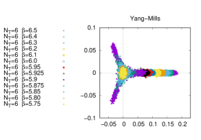
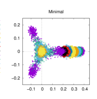
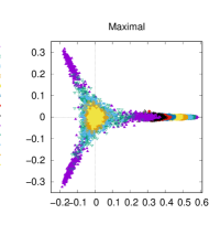
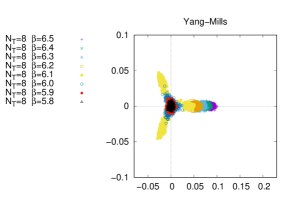
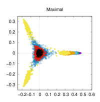
Figure 1: Distributions of the space-averaged Polyakov loop on the complex plane for the data set I: (upper three panels) for $N_{T}=6$ and $\beta=5.75,5.80,5.85,5.875,5.9,5.925,5.95,6.0,6.1,6.2,6.3,6.4,6.5$ (lower three panels) $N_{T}=8$ and $\beta=5.8,5.9,6.0,6.1,6.2,6.3,6.4,6.5$. Plots are given from left to right for the original Yang-Mills field $P_{U}^{YM}$, the restricted field in the minimal option $P_{V}^{\text{min}}$ and the restricted field in the maximal option $P_{V}^{\text{max}}$.

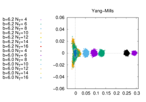
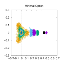
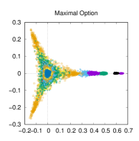
Figure 2: Distributions of the space-averaged Polyakov loop on the complex plane for the data set II: for $N_{T}=4,6,8,10,12,14,16$ at $\beta=6.2$ and $\beta=6.0$. Plots are given from left to right for the original Yang-Mills field $P_{U}^{YM}$, the restricted field in the minimal option $P_{V}^{\text{min}}$ and the restricted field in the maximal option $P_{V}^{\text{max}}$.

First, we investigate the Polyakov loop obtained by the original gauge field configurations $\{U_{x,\mu}\}$ and the restricted gauge field configurations $\{V_{x,\mu}^{\min}\}$ $\{V_{x,\mu}^{\max}\}$ in the minimal and maximal options, in order to clarify the role of the restricted fields at finite temperature. The Polyakov loop average is the order parameter associated with the center symmetry breaking. Note that the Polyakov loop average of the Yang-Mills field is conventionally used as a criterion for the confinement and deconfinement phase transition.

For the original gauge field configurations $\{U_{x,\mu}\}$, the restricted gauge field configurations in the minimal and maximal options $\{V_{x,\mu}^{\min}\}$ and $\{V_{x,\mu}^{\max}\}$, we define the respective Polyakov loop $P_{\ast}(\vec{x}\mathbf{)}$ ( $\ast=U,V^{\min},V^{\max}$ ) by

$$P_{U}() :=\frac{1}{3}\text{{tr}}\left(P\prod\limits_{t=1}^{N_{T}}U_{(\vec{x},t),4}\right),$$ (12a)

$$\ P_{V^{\min}}(\vec{x}) :=\frac{1}{3}\text{{tr}}\left(P\prod\limits_{t=1}^{N_{T}}V_{(\vec{x},t),4}^{\min}\right),$$ (12b)

$$P_{V^{\max}}(\vec{x}) :=\frac{1}{3}\text{{tr}}\left(P\prod\limits_{t=1}^{N_{T}}V_{(\vec{x},t),4}^{\max}\right),$$ (12c)

and define the space-averaged Polyakov loop $P_{\ast}$ , i.e., the value of the Polyakov loop averaged over the spatial volume by

$$P_{U} =\frac{1}{L^{3}}\sum_{\vec{x}}P_{U}(\vec{x}),$$ (13a)

$$P_{V^{\min}} =\frac{1}{L^{3}}\sum_{\vec{x}}P_{V^{\min}}(\vec{x}),\$$ (13b)

$$P_{V^{\max}} =\frac{1}{L^{3}}\sum_{\vec{x}}P_{V^{\max}}(\vec{x}),$$ (13c)

for each configuration in the complex plane.

FIG. 1 and FIG. 2 show the distributions of the space-averaged Polyakov loop $P_{\ast}$ on the complex plane obtained from the data set I and II respectively. In each figure, the three panels are arranged from left to right to show the plots measured using a set of the original gauge field configurations $P_{U}$, the restricted gauge field configurations in the minimal option $P_{V^{\min}}$ and maximal one $P_{V^{\max}}$, respectively. We find that all the distributions of the space-averaged Polyakov loops $P_{\ast}$ on the complex plane equally reflect the expected center symmetry $Z(3)$ of $SU(3)$, although they take different values option by option. Notice that the Polyakov loop average is in general complex-valued for the $SU(3)$ group. In our simulations, especially, we have used the cold start and obtained the real-valued Polyakov loop average at high temperature, as shown in FIG. 1 and FIG. 2.

Then, we measure the Polyakov-loop average $\left\langle P_{\ast}\right\rangle$ $(\ast=U,V^{\min},V^{\max})$ by simply averaging the space-averaged Polyakov loop given in FIG. 1 and FIG. 2 over the total sets of the original field configurations and the restricted field configurations in the minimal and maximal options. In what follows, the symbol $\left\langle\mathcal{O}\right\rangle$ denotes the average of the operator $\mathcal{O}$ over the ensemble of the configurations.

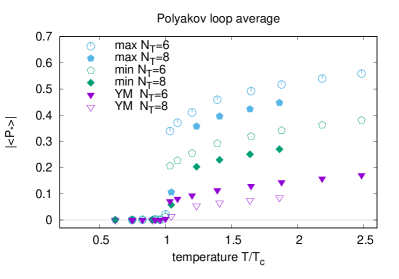
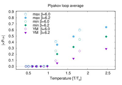
Figure 3: The Polyakov-loop averages versus temperature: The three plots for the Polyakov loop averages $\left<P_{*}\right>$ $(*=U,V^{\min},V^{\max})$ at a temperature $T$ represent from bottom to top the Polyakov loop averages for the original gauge field $U$, the restricted field $V^{\min}$ in the minimal option and the restricted field $V^{\max}$ in the maximal one, respectively. (upper panel) The plot for the data set I. (lower panel) The plots for the data set II.

FIG. 3 shows the Polyakov loop average versus the temperature determined by using Table 1 and 2. We find that the Polyakov loop averages $\left\langle P_{\ast}\right\rangle$ $(\ast=U,V^{\min},V^{\max})$ take different values option by option, namely, $\ast=U,V^{\min},V^{\max}$. It is observed that among the Polyakov loop averages $\left\langle P_{\ast}\right\rangle$ at a temperature $T$ the original gauge field $U$ gives the smallest value and that the restricted fields $V$ give larger values: $V^{\max}$ in the maximal option gives the largest value, while the restricted field $V^{\min}$ in the minimal option gives the value in between. However, the three Polyakov loop averages, $\left\langle P_{U}\right\rangle$, $\left\langle P_{V^{\min}}\right\rangle$ and $\left\langle P_{V^{\max}}\right\rangle,$ give the same critical temperature for the phase transition separating the low-temperature confined phase characterized by the vanishing Polyakov loop average $\left\langle P_{U}\right\rangle=\left\langle P_{V^{\min}}\right\rangle=\left\langle P_{V^{\max}}\right\rangle=0$ from the high-temperature deconfined phase characterized by the non-vanishing Polyakov loop average $\left\langle P_{U}\right\rangle\neq 0$, $\left\langle P_{V^{\min}}\right\rangle\neq 0$, and $\left\langle P_{V^{\max}}\right\rangle\neq 0$. We also find that the critical temperature determined from the data set I and II agrees with each other.

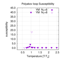
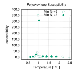
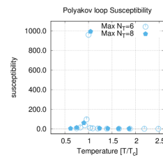
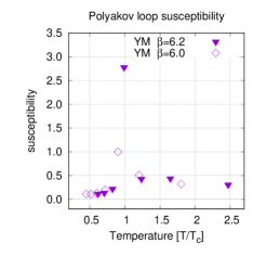
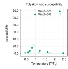
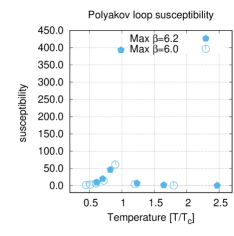
Figure 4: The Polyakov loop susceptibility versus temperature: (upper row) data set I. (lower row) data set II. The three panels in each row represent from left to right the susceptibilities calculated from the Polyakov loops of the original Yang-Mills field $P_{U}^{\text{YM}}$, the restricted field in the minimal option $P_{V}^{min}$, and the restricted field in the maximal option $P_{V}^{max}$.

In order to determine a precise location of the transition temperature, we introduce the susceptibility $\chi_{\ast}$ $(\ast=U,V^{\min},V^{\max})$ of the Polyakov loop by

$$\chi_{\ast}:=\frac{1}{L^{3}}\left[\left\langle\left|\sum_{\vec{x}}P_{\ast}(\vec{x})\right|^{2}\right\rangle-\left|\left\langle\sum_{\vec{x}}P_{\ast}(\vec{x})\right\rangle\right|^{2}\right].$$ (14)

FIG.4 gives the susceptibility versus temperature obtained from the data set I and II. They are calculated from the space-averaged Polyakov loop over the total sets of the original field configurations and the restricted field configurations in the minimal and maximal options, given in FIG. 1 and FIG. 2, respectively. These data clearly shows that both the minimal and maximal options reproduce the critical point of the original Yang-Mills field theory. Thus, the three Polyakov-loop averages give the identical critical temperature as

$$T_{c}=0.6285\text{ [in the unit }\sqrt{\sigma}\text{]}=276.5\text{ \ MeV}.$$ (15)

III.3 Static quark–antiquark potential at finite temperature

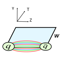
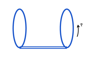
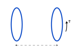
Figure 5: The set up for the measurement of the static quark-antiquark potential at finite temperature: (Left) the Wilson loop, (Center) maximally extended Wilson loop, (Right) a pair of a Polyakov loop and the anti-Polyakov loop

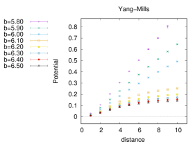
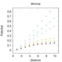
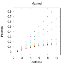
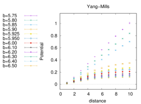
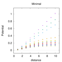
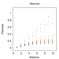
Figure 6: The static quark-antiquark potentials $V$ obtained from the maximally extended Wilson loop (16) using the data set I in the case of (upper row) $N_{T}=6$ and (lower row) $N_{T}=8$. The three panels in each row represent from left to right the original Yang-Mills field, the restricted field in the minimal option, and the restricted field in the maximal option.

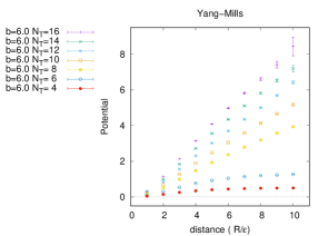
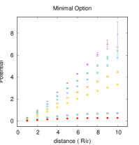
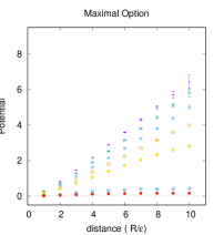
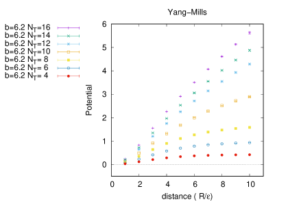
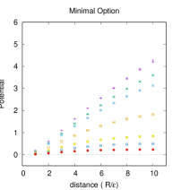
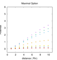
Figure 7: The static quark-antiquark potentials $V$ obtained from the maximally extended Wilson loop (16) using the data set II in the case of (upper row) $\beta=6.0$ and (lower row) $\beta=6.2$. The three panels in each row represent from left to right the original Yang-Mills field, the restricted field in the minimal option, and the restricted field in the maximal option.

Second, we investigate the static quark–antiquark potential at finite temperature. To obtain the static potential at finite temperature, we adopt the Wilson loop operator defined for the rectangular loop $C$ with the spatial length $R$ and the temporal length $\tau$ which is maximally extended in the temporal direction, i.e., $\tau=1/T$. According to the standard argument, for large $\tau$ i.e., small $T$, the static potential is obtained from the original gauge field $U$ and the restricted field $V$:

$$V(R;U) :=-\frac{1}{\tau}\log\left\langle\left\langle W_{U}\right\rangle\right\rangle=-T\log\left\langle\left\langle W_{U}\right\rangle\right\rangle,\quad$$ (16a)

$$V(R;V) :=-\frac{1}{\tau}\log\left\langle\left\langle W_{V}\right\rangle\right\rangle=-T\log\left\langle\left\langle W_{V}\right\rangle\right\rangle.$$ (16b)

In what follows, the symbol $$\left\langle\left\langle\mathcal{O}\right\rangle\right\rangle \mathcal{O}$$ denotes the average of the operator over the space-time and  ensemble of the configurations.

According to the imaginary time formalism of the quantum field theory at finite temperature $T$, the temporal (imaginary time) direction $\tau$ of the space-time has a finite length of extension $1/T$. Therefore, if the rectangular closed loop is maximally extended in the temporal direction, then it eventually reaches the boundaries at $\tau=0$ and $\tau=1/T$ which are to be identified by the periodic boundary condition. See the left and middle panels of FIG. 5.

This definition (16) of the static potential is based on an analogy with that of the Wilson loop average at zero temperature, and agrees with the static potential at zero temperature in the limit $T\rightarrow 0$. Therefore, this definition of the static potential at finite temperature is valid for low temperatures or not-so-high temperatures, but it will be problematic to use in extremely high temperatures above the critical temperature.

FIG.6 and FIG. 7 show the static potentials at various temperatures calculated according to the definition (17). The panels in the upper and lower rows of FIG. 6 show the potentials calculated respectively from configurations with $N_{t}=6$ and $N_{t}=8$ of the data set I . While, the panels in the upper and lower rows of FIG. 7 show the results calculated respectively from configurations with $\beta=6.0$ and $\beta=6.2$ of the data set II . The three static potentials are obtained by the original gauge field (Yang-Mills field), the restricted fields ($V$-fields) in the minimal and maximal options. By comparing these results, we find that the restricted fields in both options reproduce the string tension of the original Yang-Mills field. Therefore, we have shown the restricted field ($V$-field) dominance in the string tension for both options at finite temperature.

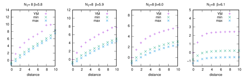
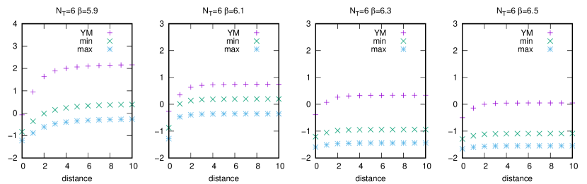
Figure 8: The static quark-antiquark potentials $\tilde{V}$ obtained from the Polyakov loop correlator using the data set II in the case of (upper row) $N_{T}=6$ for a low temperature $T<T_{c}$, and (lower row) $N_{T}=8$ for a high temperature $T>T_{c}$. The three potentials in each panel represent from top to bottom the original Yang-Mills field, the restricted field in the minimal option, and the restricted field in the maximal option.

The Wilson loop maximally extended in the temporal direction looks like a pair of the Polyakov loop $P(\vec{x})$ and the anti-Polyakov loop $P(\vec{x})^{\ast}$ (the Polyakov loop defined by the path-ordering in the reverse direction, i.e., the complex conjugate of the Polyakov loop), see the right panel of FIG 5. However, it should be remarked that the potential obtained from the maximally extended Wilson loop is different from the “potential” $\tilde{V}(R;U)$ defined from the correlation function for a pair of the Polyakov loop $P(\vec{x})$ and anti-Polyakov loop $P^{\ast}(\vec{y})$ separated by the spatial distance $R=\left\|\vec{x}-\vec{y}\right\|$ as

$$\tilde{V}(R;U) :=-T\log\left\langle\left\langle P_{U}(\vec{x})P_{U}^{\ast}(\vec{y})\right\rangle\right\rangle,$$ (17a)

$$\quad\tilde{V}(R;V) :=-T\log\left\langle\left\langle P_{V}(\vec{x})P_{V}^{\ast}(\vec{y})\right\rangle\right\rangle,$$ (17b)

where each Polyakov loop is defined by the corresponding closed loop obtained by identifying the end points at $$\tau=0 \tau=1/T \tilde{V}$$ and due to the periodic boundary condition. FIG. 8 gives the result for the measurement of at various temperatures.

In fact, it is known YHM05 ; BW79 that the Polyakov loop correlation function which is related to the partition function in the presence of a quark at $\vec{x}$ and an anti-quark at $\vec{y}$ is decomposed into the singlet and the adjoint combinations in the color space:

$$\left\langle\left\langle P_{U}(\vec{x})P_{U}^{\ast}(\vec{y})\right\rangle\right\rangle\simeq e^{-F_{q\bar{q}}/T}$$

$$=\frac{1}{N_{c}^{2}}e^{-F^{(S)}/T}+\frac{N_{c}^{2}-1}{N_{c}^{2}}e^{-F^{(A)}/T},$$ (18)

where $F^{(S)}$ and $F^{(A)}$ are the free energies in the singlet channel and the adjoint channel respectively. The left-hand side of (18) is gauge-invariant for arbitrary $\vec{x}$ and $\vec{y}$ by construction. However, the decomposition in the right-hand side of (18) is gauge-dependent and thus should be taken with care. In sharp contrast to $\tilde{V}$, the potential $V$ obtained from the Wilson loop is color singlet and gauge-independent object.

III.4 Chromo-flux tube at finite temperature

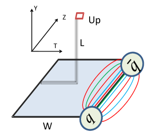
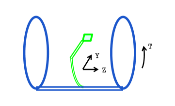
Figure 9: The set up for the measurement of the chromo-fluxes. (Left) The graphical representation of the operator $\text{tr}\left(WLU_{p}L^{\dagger}\right)$. (Right) The operator $\text{tr}\left(WLU_{p}L^{\dagger}\right)$ with the maximally extended Wilson loop $W$.

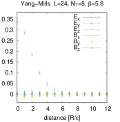
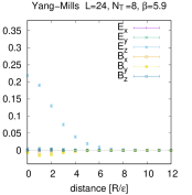
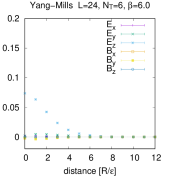
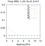
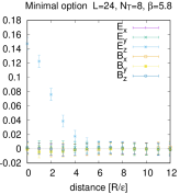
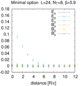
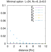
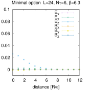
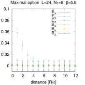
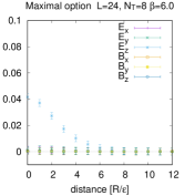
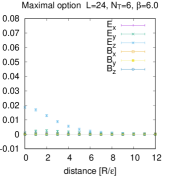
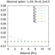
Figure 10: The components of the chromo flux obtained from the data set I: $E_{x}=F^{q\bar{q}}_{14}$, $E_{y}=F^{q\bar{q}}_{24}$, $E_{z}=F^{q\bar{q}}_{34}$, $B_{x}=F^{q\bar{q}}_{23}$, $B_{y}=F^{q\bar{q}}_{31}$, $B_{z}=F^{q\bar{q}}_{12}$. The three panels in the same column correspond to the different options: (top row) the original Yang-Mills field, (mid row) the restricted field in the minimal option, and (bottom row) the restricted field in the maximal option. In the four panels in each row, the left two are at low temperatures in the confinement phase $T<T_{c}$, while the right two are at high temperatures in the deconfinement phase $T_{c}<T$.

We proceed to investigate the dual Meissner effect at finite temperature. For this purpose, we use the gauge-invariant correlation function which is the same as that used at zero temperature GMO90 . We measure the chromo-flux created by a quark-antiquark pair, which is represented by the maximally extended Wilson loop $W$ given in the center panel of FIG.5. The chromo-field strengths, i.e., the field strengths of the chromo-flux created by the Wilson loop of the original Yang-Mills field, the restricted field in the minimal and maximal options are measured by using the three kind of the probes defined by

$$F_{\mu\nu}^{\text{YM}}(y) =\sqrt{\frac{\beta}{6}}\rho_{{}_{U_{P}}}(y)\text{, \ }$$ (19a)

$$\rho_{{}_{U_{P}}}^{\text{YM}}(y) :=\frac{\left\langle\left\langle\mathrm{tr}\left(WL[U]U_{p}(y)L^{{\dagger}}[U]\right)\right\rangle\right\rangle}{\left\langle\left\langle\mathrm{tr}\left(W\right)\right\rangle\right\rangle}$$

$$-\frac{1}{N_{c}}\frac{\left\langle\left\langle\mathrm{tr}\left(U_{p}(y)\right)\mathrm{tr}\left(W\right)\right\rangle\right\rangle}{\left\langle\left\langle\mathrm{tr}\left(W\right)\right\rangle\right\rangle}\text{ },$$ (19b)

$$\text{\ }F_{\mu\nu}^{\text{min}}(y) =\sqrt{\frac{\beta}{6}}\rho_{{}_{V_{P}^{\min}}}(y)\text{, }$$ (20a)

$$\rho_{V_{p}}^{\min}(y) :=\frac{\left\langle\left\langle\mathrm{tr}\left(WL[V^{\min}]V_{p}^{\min}(y)L^{{\dagger}}[V^{\min}]\right)\right\rangle\right\rangle}{\left\langle\left\langle\mathrm{tr}\left(W\right)\right\rangle\right\rangle}$$

$$-\frac{1}{N_{c}}\frac{\left\langle\left\langle\mathrm{tr}\left(V_{p}^{\min}(x)\right)\mathrm{tr}\left(W\right)\right\rangle\right\rangle}{\left\langle\left\langle\mathrm{tr}\left(W\right)\right\rangle\right\rangle},$$ (20b)

$$\text{\ \ \ }F_{\mu\nu}^{\max}(y) =\sqrt{\frac{\beta}{6}}\rho_{{}_{V_{P}^{\max}}}(y)\text{, }$$ (21a)

$$\rho_{{}_{V_{P}}}^{\max}(y) :=\frac{\left\langle\left\langle\mathrm{tr}\left(WL[V^{\max}]V_{p}^{\max}(y)L^{{\dagger}}[V^{\max}]\right)\right\rangle\right\rangle}{\left\langle\left\langle\mathrm{tr}\left(W\right)\right\rangle\right\rangle}$$

$$-\frac{1}{N_{c}}\frac{\left\langle\left\langle\mathrm{tr}\left(V^{\max}(x)\right)\mathrm{tr}\left(W\right)\right\rangle\right\rangle}{\left\langle\left\langle\mathrm{tr}\left(W\right)\right\rangle\right\rangle},$$ (21b)

where $$U_{p} V_{p}^{\min} V_{p}^{\max} U V^{\min} V^{\max} L W U_{p} \ V_{p}^{\min} V_{p}^{\max} R\times N_{T} \ R=7 N_{T} z-t t R z z=0, 0\leq t \leq N_{T} z=R 0\leq t \leq N_{T} y t_{\text{mid}}= N_{T}/2-1 z_{\text{mid}}=3 L L^{{\dagger}} z=z_{mid} t=0 z-t z=z_{mid} t=t_{mid} y 0 Y x=0,y z_{mid} t_{mid}) 0\leq y\leq Y\,$$, , and represent plaquette variables for the field strength made of the Yang-Mills fields , the restricted fields in the minimal and maximal options, and , respectively, and is the Schwinger line connecting the source and the probes, , , and , which is introduced to guarantee the gauge-invariance. FIG.9 shows the graphical representation of the connected correlation Eqs.(19)–(21). We prepare the maximally extended Wilson loop of the size with and being the size of the temporal direction where the Wilson loop is placed at plane (see FIG.9), and ae quark and an anti-quark are placed along the temporal direction (-direction) at the distance in the -direction. When we introduce the coordinates relative to the Wilson loop, the quark and antiquark are respectively represented by the segments, and , in the Wilson loop, respectively. The coordinates in Eqs.(19)–(21) represents the amount of shift from the Wilson loop. We measure the chromo flux at the midpoint of the Wilson loop, and , i.e., the Schwinger line () is connected at the point , in the plane and extended to the center of the Wilson loop, , . The plaquette is displaced along the -direction from the center of the Wilson loop (the point of the distance ) to the point of the distance , i.e., (, , , .

The three kind of the chromo fluxes for the Yang-Mills fields and the restricted fields in the minimal and maximal options are distinguished by using different probes made of the Yang-Mills fields and the restricted fields in the minimal and maximal options, $L[U]U_{p}L^{{\dagger}}[U]$, $L[V^{\min}]V_{p}^{\min}L^{{\dagger}}[V^{\min}]$, and $L[V^{\max}]V_{p}^{\max}L^{{\dagger}}[V^{\max}]$,  respectively. Indeed, in the naive continuum limit, the connected correlations are reduced to

$$\rho_{{}_{U_{P}}}^{\text{YM}}\overset{\varepsilon\rightarrow 0}{\simeq}g\varepsilon^{2}\left\langle\mathcal{F}_{\mu\nu}[U]\right\rangle_{q\bar{q}}$$

$$:=\frac{\left\langle\left\langle\mathrm{tr}\left(g\varepsilon^{2}\mathcal{F}_{\mu\nu}[U]L[U]^{{\dagger}}WL[U]\right)\right\rangle\right\rangle}{\left\langle\left\langle\mathrm{tr}\left(W\right)\right\rangle\right\rangle}+O(\varepsilon^{4}),$$ (22)

$$\rho_{{}_{V_{P}}}^{\min}\overset{\varepsilon\rightarrow 0}{\simeq}g\varepsilon^{2}\left\langle\mathcal{F}_{\mu\nu}[V^{\min}]\right\rangle_{q\bar{q}}$$

$$:=\frac{\left\langle\left\langle\mathrm{tr}\left(g\varepsilon^{2}\mathcal{F}_{\mu\nu}[V^{\min}]L[V^{\min}]^{{\dagger}}WL[V^{\text{min}}]\right)\right\rangle\right\rangle}{\left\langle\left\langle\mathrm{tr}\left(W\right)\right\rangle\right\rangle}$$

$$+O(\varepsilon^{4}),$$ (23)

$$\rho_{{}_{V_{P}}}^{\max}\overset{\varepsilon\rightarrow 0}{\simeq}g\varepsilon^{2}\left\langle\mathcal{F}_{\mu\nu}[V^{\max}]\right\rangle_{q\bar{q}}$$

$$:=\frac{\left\langle\left\langle\mathrm{tr}\left(g\varepsilon^{2}\mathcal{F}_{\mu\nu}[V^{\max}]L[V^{\max}]^{{\dagger}}WL[V^{\max}]\right)\right\rangle\right\rangle}{\left\langle\left\langle\mathrm{tr}\left(W\right)\right\rangle\right\rangle}$$

$$+O(\varepsilon^{4})\text{ }.$$ (24)

FIG.10 exhibits the chromo fluxes measured by using Eqs.(19)–(21) for the data set I. Note again that the physical unit (the lattice spacing) is different $\beta$ by $\beta$ and we cannot directly compare measured values between the different lattice, because the temperature varies by changing $\beta$ for the fixed size of the lattice and the lattice spacing is a function of $\beta$. The three panels from top to bottom in each column show the option dependence of the chromo fluxes obtained for the Yang-Mills field, the restricted field in the minimal option and the restricted field in the maximal options with the lattice size and the gauge coupling being fixed. The four panels from left to right in each row show the temperature dependence of the chromo fluxes at different temperatures in the same option. At a low-temperature in the confinement phase, $T<T_{c}$, we observe that only the component $E_{z}$ of the chromoelectric flux in the direction connecting a quark and antiquark pair is non-vanishing, while the other components take vanishing values, see the left two panels in each row of FIG. 10. At a high-temperature in the deconfinement phase, $T>T_{c}$, we observe that the component $E_{z}$ of the chromoelectric flux becomes much smaller as the temperature increases and that the other components still take vanishing values, see the right two panels in each row of FIG. 10. The magnitude of the chromoelectric field decreases as the temperature increases, and rapidly falls off when the temperature exceeds the critical temperature. Therefore, the flux tube gradually disappears above the critical temperature.

Thus, the results of FIG.10 give the numerical evidence for the disappearance of the dual Meissner effect in the high-temperature deconfinement phase. These results should be compared with similar analyses for the Yang-Mills field at finite temperature by using a pair of Polyakov loops Cea2016 ; Cea2018 . Our results are consistent with them.

III.5 Magnetic–monopole current and dual Meissner effect at finite temperature

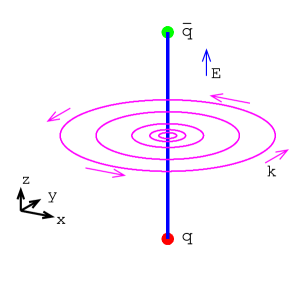
Figure 11: The magnetic–monopole current $k$ induced around the chromo-flux tube created by a quark-antiquark pair.

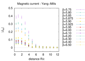
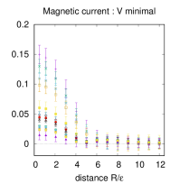
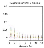
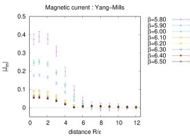
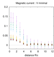
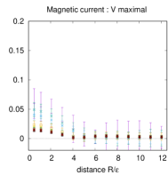
Figure 12: The magnitude $|J_{m}|=\sqrt{k_{\mu}k_{\mu}}$ of the induced magnetic current $k_{\mu}$ ($J_{m,\mu}$) around the flux tube connecting a quark-antiquark pair as a function of the distance $y$ from the $z$ axis for various values of $\beta$. (Upper row) The results for $N_{T}=6$ from data set I. (Upper row) The results for $N_{T}=8$ from data set I. The three panels in each row represent from left to right the original Yang-Mills field, the restricted field in the minimal option, and the restricted field in the maximal option.

Finally, we investigate the dual Meissner effect by measuring the magnetic–monopole current $k$ induced around the chromo-flux tube created by a quark-antiquark pair, see FIG.11. We use the magnetic–monopole current $k$ defined by

$$k_{\mu}^{\text{YM}}(x) =\frac{1}{2}\varepsilon_{\mu\nu\alpha\beta}\left(F_{\alpha\beta}^{YM}(x+\hat{\nu})-F_{\alpha\beta}^{YM}(x)\right),$$ (25a)

$$k_{\mu}^{\text{min}}(x) =\frac{1}{2}\varepsilon_{\mu\nu\alpha\beta}\left(F_{\alpha\beta}^{\min}(x+\hat{\nu})-F_{\alpha\beta}^{\min}(x)\right),$$ (25b)

$$k_{\mu}^{\text{max}}(x) =\frac{1}{2}\varepsilon_{\mu\nu\alpha\beta}\left(F_{\alpha\beta}^{\max}(x+\hat{\nu})-F_{\alpha\beta}^{\max}(x)\right),$$ (25c)

where $F_{\mu\nu}^{(\ast)}$ are the field strength defined by Eqs.(19)–(21). This definitions satisfy the conserved current, i.e., $\partial_{\mu}k_{\mu}^{(\ast)}(x):=\sum_{\mu}\left(k_{\mu}^{(\ast)}(x+\hat{\mu})-k_{\mu}^{(\ast)}(x)\right)\equiv 0$. There is a general belief that the magnetic–monopole current (25) must vanish due to the Bianchi identity as far as there exist no singularities in the gauge potential $A$. In fact, if the field strength $F^{(\ast)}$ was written in the exact form $F^{(\ast)}=dA^{(\ast)}$ using the differential form, the magnetic–monopole current would vanish $k^{(\ast)}:={}^{\ast}dF={}^{\ast}ddA=0$ due to $dd\equiv 0$. This is not the case in the Yang-Mills theory. We show that the magnetic–monopole current defined in this way (25) can be the order parameter for the confinement/deconfinement phase transition, as suggested from the dual superconductivity hypothesis. FIG. 12 shows the result of the measurements of the magnitude $\sqrt{k_{\mu}k_{\mu}}$ of the induced magnetic current $k_{\mu}$ obtained according to (25) for various temperatures ($\beta$). The current decreases as the temperature becomes higher and eventually vanishes above the critical temperature for both options. We observe respectively the appearance and disappearance of the magnetic monopole current in the low temperature phase and high temperature phase.

IV Conclusion

Using a new formulation of the Yang-Mills theory on a lattice, we have investigated the confinement/deconfinement phase transition at finite temperature in the $SU(3)$ Yang-Mills theory from the viewpoint of the dual superconductivity. We have compared the two possible realizations of the dual superconductivity at finite temperature by adopting the two possible options in the $SU(3)$ Yang-Mills theory, i.e., the non-Abelian dual superconductivity in the minimal option and the conventional Abelian dual superconductivity in the maximal one. In both options, we have succeeded even at finite temperature to extract the restricted field variable ($V$-field) from the original Yang-Mills field variable as the dominant mode for confining quarks in the fundamental representation, which could be called the restricted field dominance at finite temperature. In both options, moreover, we have investigated the dual Meissner effect to show that the chromoelectric flux tube appears in the confining phase, but it disappears in the deconfining phase. Thus, both options can be adopted to give the low-energy effective description for quark confinement of the original Yang-Mills theory.

In fact, we have given the numerical evidences for the restricted field dominance. First, we have investigated the Polyakov loop averages at finite temperature and have shown that that the Polyakov loop average $\langle P_{V}\rangle$ of the restricted field $V$ gives the same critical temperature $T_{c}$ as that detected by the Polyakov loop average $\langle P_{U}\rangle$ of the original gauge field $U$: $\langle P\rangle=0$ for $T<T_{c}$ and $\langle P\rangle\neq 0$ for $T>T_{c}$.

Next, we have investigated the static quark potential at finite temperature by using the maximally extended Wilson loop and the correlation function for a pair of the Polyakov loop and the anti-Polyakov loop. We have found the restricted field ($V$-field) dominance in the string tension at finite temperature for both options: the string tension calculated from the restricted field reproduces that from the original Yang-Mills theory. Both measurements by using the Wilson loop and the Polyakov loop are in good agreements. When the temperature exceeds the critical temperature, the string tension rapidly vanishes as the temperature increases. The restricted fields in both options reproduce the center symmetry restoration/breaking of the original Yang-Mills theory, and give the same critical temperature of the confining/deconfining phase transition.

However, the Polyakov loop average cannot be the direct signal of the dual Meissner effect or magnetic monopole condensation. Therefore, it is important to find an order parameter which enables one to detect the dual Meissner effect directly. In view of these, we have measured the chromoelectric and chromomagnetic flux for both the original field and the restricted fields in the two options. In the low–temperature confined phase $T<T_{c}$, we have obtained the numerical evidences of the dual Meissner effect in the $SU(3)$ Yang-Mills theory, namely, the squeezing of the chromoelectric flux tube created by a quark-antiquark pair and the associated magnetic–monopole current induced around the flux tube. In the high–temperature deconfined phase $T>T_{c}$, on the other hand, we have observed the disappearance of the dual Meissner effect, namely, no more squeezing of the chromoelectric flux tube detected by non-vanishing component in the chromoelectric flux and the vanishing of the magnetic-monopole current associated with the chromo-flux tube. We have confirmed that the dual Meissner effect can be described by the restricted field alone for both options. Therefore, we have confirmed the restricted field dominance in the dual Meissner effect even at finite temperature. Thus, we have given the evidences that the confinement/deconfinement phase transition at finite temperature is caused by appearance/disappearance of the dual superconductivity for the $SU(3)$ Yang-Mills theory.

Acknowledgement

This work was supported by Grant-in-Aid for Scientific Research, JSPS KAKENHI Grant Number (C) No. 24540252, No.15K05042, and No.19K03840. A.S. was supported also in part by JSPS Grant-in-Aid for Scientific Research (S) 22224003. The numerical calculations are supported by the Large Scale Simulation Program of High Energy Accelerator Research Organization (KEK): No.12/13-20(FY2012-13), No.13/14-23(FY2013-14), No.14/15-24(FY2014-15), and No.16/17-20(FY2016-17)

References

-
(1)
Y. Nambu,
Phys. Rev. D10, 4262–4268 (1974).
G. ’t Hooft, in: High Energy Physics, edited by A. Zichichi (Editorice Compositori, Bologna, 1975).
S. Mandelstam, Phys. Report 23, 245–249 (1976). - (2) K.-I. Kondo, T. Murakami and T. Shinohara, Prog. Theor. Phys. 115, 201–216 (2006). [hep-th/0504107] K.-I. Kondo, T. Murakami and T. Shinohara, Eur. Phys. J. C42, 475–481 (2005). [hep-th/0504198] K.-I. Kondo, T. Shinohara and T. Murakami, Prog. Theor. Phys. 120, 1–50 (2008). arXiv:0803.0176 [hep-th]
- (3) S. Kato, K.-I. Kondo, T. Murakami, A. Shibata, T. Shinohara and S. Ito, Phys. Lett. B632, 326–332 (2006). [hep-lat/0509069]
- (4) K.-I. Kondo, A. Shibata, T. Shinohara, T. Murakami, S. Kato, S. Ito, Phys. Lett. B669, 107–118 (2008). arXiv:0803.2451 [hep-lat]
- (5) A. Shibata, K.-I. Kondo and T. Shinohara, Phys. Lett. B691, 91–98 (2010). arXiv:0911.5294 [hep-lat]
- (6) K.-I. Kondo, S. Kato, A. Shibata and T. Shinohara, Phys. Rep. 579, 1–226 (2015). arXiv:1409.1599 [hep-th].
- (7) G. ’t Hooft, Nucl.Phys. B190 [FS3], 455–478 (1981).
- (8) A. Kronfeld, M. Laursen, G. Schierholz and U.-J. Wiese, Phys. Lett. B198, 516–520 (1987).
- (9) K.-I. Kondo, Phys. Rev. D 77, 085029 (2008). arXiv:0801.1274 [hep-th]
- (10) K.-I. Kondo and A. Shibata, arXiv:0801.4203 [hep-th]
- (11) K.-I. Kondo, A. Shibata, T. Shinohara, and S. Kato, Phys. Rev. D83, 114016 (2011). arXiv:1007.2696 [hep-th]
- (12) A. Shibata, S. Kato, K.-I. Kondo, T. Shinohara and S. Ito, PoS(LATTICE 2008) 268, arXiv:0810.0956 [hep-lat]
- (13) A. Shibata, K.-I. Kondo, S.Kato, S. Ito, T. Shinohara and N. Fukui, PoS LAT2009 (2009) 232, arXiv:0911.4533 [hep-lat].
- (14) A. Shibata, K.-I. Kondo, S. Kato and T. Shinohara, PoS(Lattice 2010) 286
- (15) A. Shibata, K.-I. Kondo, S. Kato and T. Shinohara, Phys. Rev. D87, 054011 (2013). arXiv:1212.6512 [hep-lat]
- (16) Y. Matsubara, S. Ejiri and T. Suzuki, Nucl. Phys. B. Proc. Suppl. 34, 176–178 (1994).
- (17) M. S. Cardaci, P. Cea, L. Cosmai, R. Falcone and A. Papa, Phys. Rev. D 83, 014502 (2011) [arXiv:1011.5803 [hep-lat]]
- (18) N. Cardoso, M. Cardoso and P. Bicudo, Phys. Rev. D 84, 054508 (2011) [arXiv:1107.1355 [hep-lat]].
- (19) P. Cea, L. Cosmai and A. Papa, Phys. Rev. D86, 054501 (2012). arXiv:1208.1362 [hep-lat]
- (20) P. Cea, L. Cosmai, F. Cuteri, and A. Papa, Phys. Rev. D89, 094505 (2014). arXiv:1404.1172 [hep-lat]
-
(21)
Y.M. Cho,
Unpublished preprint, MPI-PAE/PTh 14/80 (1980).
Y.M. Cho, Phys. Rev. Lett. 44, 1115–1118 (1980). - (22) L. Faddeev and A.J. Niemi, Phys. Lett. B449, 214–218 (1999). [hep-th/9812090] L. Faddeev and A.J. Niemi, Phys. Lett. B464, 90–93 (1999). [hep-th/9907180] T.A. Bolokhov and L.D. Faddeev, Theoretical and Mathematical Physics, 139, 679–692 (2004).
- (23) Y.M. Cho, Phys. Rev. D 21, 1080 (1980). Phys. Rev. D 23, 2415 (1981); Y.S. Duan and M.L. Ge, Sinica Sci., 11, 1072(1979); L. Faddeev and A.J. Niemi, Phys. Rev. Lett. 82, 1624 (1999); S.V. Shabanov, Phys. Lett. B 458, 322 (1999). Phys. Lett. B 463, 263 (1999).
- (24) A. Shibata, S. Kato, K.-I. Kondo, T. Shinohara and S. Ito, POS(LATTICE2007) 331, arXiv:0710.3221 [hep-lat]
-
(25)
N. Cundy, Y.M. Cho, W. Lee, and J. Leem,
Phys. Lett. B729, 192–198 (2014). arXiv:1307.3085 [hep-lat]
N. Cundy, Y.M. Cho, and W. Lee, PoS LATTICE2013 (2013) 471, arXiv:1311.3029 [hep-lat]
N. Cundy, W. Lee, J. Leem, Y.M. Cho, PoS LATTICE2012 (2012) 213, arXiv:1211.0664 [hep-lat] - (26) S. Gongyo, T. Iritani, and H. Suganuma, Phys. Rev. D86, 094018 (2012). e-Print: arXiv:1207.4377 [hep-lat]
- (27) N. Sakumichi and H. Suganuma, Phys.Rev. D90, 111501 (2014), e-Print: arXiv:1406.2215 [hep-lat]
- (28) S. Ito, S. Kato, K.-I. Kondo, T. Murakami, A. Shibata and T. Shinohara, Phys. Lett. B645, 67–74 (2007). [hep-lat/0604016]
- (29) A. Shibata, S. Kato, K.-I. Kondo, T. Murakami, T. Shinohara and S. Ito, Phys. Lett. B653, 101–108 (2007). arXiv:0706.2529 [hep-lat]
- (30) S. Kato, K.-I. Kondo, A. Shibata and T. Shinohara, PoS(LAT2009) 228.
- (31) P. Cea and L. Cosmai, Phys. Rev. D52, 5152 (1995) P. Cea and L. Cosmai, Phys. Lett. B349, 343 (1995).
- (32) P. Cea, L. Cosmai and A. Papa, Phys. Rev. D86, 054501 (2012). P. Cea, L. Cosmai, F. Cuteri, and A. Papa, Phys. Rev.D89, 049505 (2014).
- (33) S. Kato, K.-I. Kondo, and A. Shibata, Phys. Rev. D91, 034506 (2015). arXiv:1407.2808 [hep-lat]
- (34) A. Shibata, K.-I. Kondo, S. Nishino, T. Sasago, and S. Kato, PoS (Confinement2018) 269, arXiv:1903.10487 [hep-lat] , CHIBA-EP-232, KEK Preprint 2018-78 S. Nishino, K.-I. Kondo, A. Shibata, T. Sasago, and S. Kato, Eur.Phys.J. C79 (2019) no.9, 774, arXiv:1903.10488 [hep-lat], CHIBA-EP-236, KEK Preprint 2018-82
- (35) T. Suzuki and I. Yotsuyanagi, Phys. Rev. D42, 4257–4260 (1990).
- (36) H. Shiba and T. Suzuki, Phys. Lett. B333, 461–466 (1994). [hep-lat/9404015]
- (37) J.D. Stack, S.D. Neiman and R. Wensley, Phys. Rev. D50, 3399–3405 (1994). [hep-lat/9404014]
- (38) R. Matsudo, A. Shibata, S. Kato, K.-I. Kondo, Phys. Rev. D100, 014505, arXiv:1904.09388 [hep-lat] A. Shibata , R. Matsudo, S. Kato, K.-I. Kondo, PoS LATTICE2018 (2018) 254, arXiv:1812.05827 [hep-lat]
- (39) A. Shibata, K.-I. Kondo, S. Kato and T. Shinohara, PoS LATTICE2012 (2012) 215, arXiv:1212.2835 [hep-lat]
- (40) A. Shibata, K.-I. Kondo, S. Kato, T.Shinohara, PoS LATTICE2013 (2014), arXiv:1403.3809 [hep-lat]
- (41) A. Shibata, K.-I. Kondo, S. Kato, T.Shinohara, PoS LATTICE2014 (2015) 340, arXiv:1501.06271 [hep-lat]
- (42) A. Shibata, K.-I. Kondo, S. Kato, T.Shinohara, PoS LATTICE2015 (2016) 320, arXiv:1512.03695 [hep-lat]
- (43) A. Shibata, K.-I. Kondo, S. Kato, and T. Shinohara, PoS LATTICE2016 (2017) 345, :arXiv:1701.02442 [hep-lat]
- (44) A. Shibata, K.-I. Kondo, S. Kato, and T. Shinohara, Proceedings of Origin of Mass and Strong Coupling Gauge Theories (SCGT15), 168-174 (2018) ; Int.J.Mod.Phys. A32 (2017) no.36, 1747016, : arXiv:1511.04155 [hep-lat]
- (45) A. Shibata, K.-I. Kondo, S. Kato and T. Shinohara, PoS ConfinementX (2012) 052, arXiv:1302.6865 [hep-lat]
- (46) A. Shibata, K.-I. Kondo, S. Kato, PoS Confinement2018 (2019) 061, arXiv:1812.06797 [hep-lat]
- (47) R.G. Edwards, Urs. M. Heller and T.R. Klassen, Nucl. Phys. B517 (1998) 377-392
- (48) M. Albanese et al. (APE Collaboration), Phys. Lett. B192, 163–169 (1987).
- (49) K. Yagi, T. Hatsuda and Y. Miake, Quark-Gluon Plasma (Cambridge Univ. press, Cambridge, 2005).
- (50) L.S. Brown and W.I. Weisberger, Phys.Rev. D20 (1979) 3239
-
(51)
A. Di Giacomo, M. Maggiore and S. Olejnik,
Nucl. Phys. B347, 441–460 (1990).
A. Di Giacomo, M. Maggiore and S. Olejnik, Phys. Lett. B236, 199–202 (1990). - (52) P. Cea, L. Cosmai, F.Cuteri, A. Papa, JHEP 1606 (2016) 033
- (53) P.Cea, L.Cosmai, F.Cuteri, A.Papa, EPJ Web Conf. 175 (2018) 12006