Calibration of Local-Stochastic and Path-Dependent Volatility Models to Vanilla and No-Touch Options

Abstract

We propose a generic calibration framework to both vanilla and no-touch options for a large class of continuous semi-martingale models. The method builds upon the forward partial integro-differential equation (PIDE) derived in Hambly et al. (2016), A forward equation for barrier options under the Brunick & Shreve Markovian projection, Quant. Finance, 16 (6), 827–838, which allows fast computation of up-and-out call prices for the complete set of strikes, barriers and maturities. It also utilises a novel two-state particle method to estimate the Markovian projection of the variance onto the spot and running maximum. We detail a step-by-step procedure for a Heston-type local-stochastic volatility model with local vol-of-vol, as well as two path-dependent volatility models where the local volatility component depends on the running maximum. In numerical tests we benchmark these new models against standard models for a set of EURUSD market data, all three models are seen to calibrate well within the market no-touch bid–ask.

1 Introduction

For derivative pricing models to be useful in practice, they need to allow calibration to the market prices of liquid contracts, as well as exhibit a dynamic behaviour consistent with that of the underlying and with future options quotes. Vanilla options prices provide a snapshot of the market implied distributions of the underlying which is the key ingredient for pricing European options, but they provide limited information about the joint law of the underlying observed at different times, which is needed for pricing path dependent options. There is evidence (see, e.g., [2]) that the market prices of contracts with barrier features contain additional information on the dynamic behaviour of the volatility surface not already seen in vanilla quotes. The topic of this paper is hence the simultaneous calibration of volatility models to European call and no-touch (or, more generally, barrier) options.

The case of calibration to vanilla options, i.e. European calls and puts, has been considered extensively in the literature. The seminal work of Dupire [13] gives a constructive solution to the calibration problem for local volatility (LV) models, which can perfectly match call prices for any strike and maturity. Nowadays, local-stochastic volatility (LSV) models are in widespread use in financial institutions because of their ability to calibrate exactly to vanilla options due to the local volatility component while embedding a stochastic variance component, which improves the dynamic properties. The calibration problem of LSV models to vanilla quotes is reviewed already in [34], and is addressed, more recently, in the works of Guyon and Henry-Labordère [22, 23] by a particle method, and in [36] by solution of a nonlinear Fokker-Planck PDE; see also [10, Section 6.8].

In addition to call options, practitioners are increasingly interested in including the quotes of touch options in the set of calibration instruments, which will improve the pricing and risk-management of exotic contracts with barrier features. In some markets, for example in foreign exchange, the next most visible layer of option prices after the European vanilla prices are the American barrier options (for example products such as one-touch, double no-touch and vanilla knock-out options). Observation and model parameter adjustment derived from these prices is a well-established part of model calibration for short-dated FX options.

A few published works already address this question for different model classes: Crosby and Carr [9] consider a particular class of jump models which gives a calibration to both vanillas and barriers; Pironneau [33] proves that an adaptation of the Dupire equation is valid for a given barrier level, under the local volatility model.

This paper addresses the simultaneous calibration to vanilla and barrier (specifically, no-touch) options systematically for a wide class of volatility models. The focus is less on the calibration of a particular model – although we do calibrate three different new models – but on a methodology which allows the efficient calibration of any volatility model.

We assume that interest rates are deterministic. We take the Brunick–Shreve mimicking point of view from [6] that the joint law of a stock price and its running maximum, or equivalently, barrier prices for all strikes, barriers levels and maturities, can be reproduced by a one-factor model with a deterministic volatility function of the spot, the running maximum and time. This is a natural extension of Gyöngy’s result in [24] that the stock price distribution, or equivalently, call prices for all strikes and maturities, can be reproduced with a deterministic volatility function of the spot and time. In the latter case, this volatility function is the expectation of the variance process conditional on the spot price, while in the path-dependent case the expectation is also conditional on the path-dependent quantity, here the running maximum. These conditional expectations are often referred to as Markovian projections.

In the vanilla case, exact calibration is guaranteed if the Markovian projection of the instantaneous variance onto the spot coincides with the squared local volatility function derived from vanilla quotes by Dupire’s formula. Conversely, given the local volatility, model prices can be computed by the forward Dupire PDE, formulated in strike and maturity. The estimation of the local volatility from observed prices is an ill-posed inverse problem, and regularisation approaches have been proposed, e.g., in [27], [14], or [12]. If the underlying model to be calibrated is not itself a local volatility model, the Dupire PDE can still be used to compute the model prices by utilising the mimicking result, i.e., the Dupire PDE with the Markovian projection of the instantaneous variance onto the spot as diffusion coefficient gives the correct model prices. The conditional expectation of the stochastic variance under the desired model can be estimated, e.g., by the particle method in [23, 22].

The natural extension of the forward Dupire PDE for calls to a forward equation for barrier option prices, with strike, barrier level and maturity as independent variables, is the forward PIDE derived in [26]. It has as diffusion coefficient a volatility function of spot, running maximum, and time, which we view as a ‘code book’ for barrier option prices, a name coined in [8] for local volatility and European options. We re-iterate that the underlying diffusion can be a general continuous stochastic process. Specifically, the variance process does not need to contain the running maximum in its parametrisation. The link between the original model and this path-dependent volatility is given by Corollary 3.10 in [6] (see also (2.9) below).

We investigate as example a Heston-type LSV model with a local volatility component as well as a stochastic volatility with simple parametric, spot- and time-dependent vol-of-vol (LSV-LVV). Hence, we can perform a best-fit of the vol-of-vol function to no-touch options at each quoted maturity while ensuring perfect calibration to vanilla options through the local volatility function. The tests show that the calibrated LSV-LVV model prices no-touch options well within the market bid–ask spread for all barrier levels and maturities. The approach can easily be generalised to other types of stochastic volatility diffusions.

We also construct a “local maximum volatility”, i.e. a spot and running maximum dependent volatility function (LMV) consistent with market prices of calls and no-touches by solving an inverse problem for the PIDE discussed above using regularisation. The calibration of this maximum-dependent local volatility function using the forward PIDE is inspired by, and extends, the literature on the local volatility model calibration, see e.g. [27, 14, 12]. We then consider an extension of the model in the spirit of LSV models, i.e., a local maximum-dependent volatility function (LMSV) multiplied by a stochastic volatility. These two models fall into the class of path-dependent volatility models and can be useful to replicate a market’s spot-volatility dynamics as explained in [21].

In the calibration of the LSV-LVV and LMSV models, one can compute the Markovian projection of the stochastic variance by either extending the particle method introduced in [23, 22] or by solving the Kolmogorov forward PDE for the joint density of $\mathopen{}\mathclose{{}\left(S_{t},M_{t},V_{t}}\right)$, the spot, maximum and volatility, numerically. In our approach, we rely on a two-dimensional particle method (in $(S_{t},M_{t})$) as it offers a straightforward extension to additional stochastic factors. The computationally most expensive part is, as often, retrieval of the neighbouring particles, for which we propose a binary tree search, specifically on a $k$-d tree. The use of $k$-d trees for particle method calibration is a novel approach which can easily be generalised to higher-dimensional state spaces.

The remainder of this paper is organised as follows. In Section 2, we define the models and calibration condition for up-and-out barrier option quotes. Section 3 presents an efficient numerical solution of the forward PIDE for barrier options, which is central for the algorithms in this paper. In Section 4, we present a possible calibration algorithm for the path-dependent volatility (LMV) model by forward PIDE and regularised gradient-based optimisation. Then, in Section 4.3 specifically, we use again a particle method to calibrate the LMSV model by Markovian projection. Section 5 makes use of a Markovian projection with a two-dimensional conditional state of spot and running maximum for the LSV-LVV model and combines it with the forward PIDE for barrier options in order to best-fit no-touch quotes while perfectly calibrating vanilla market prices. The calibration results for all these models are presented and compared in Section 6. Section 7 concludes with a brief discussion.

2 Models and calibration conditions

We consider a spot exchange rate $S_{t}$ associated with the currency pair FORDOM, which is the amount of units of domestic currency DOM needed to buy one unit of foreign currency FOR at time $t$. We assume the existence of a filtered probability space ($\Omega$, $\mathcal{F},\mathopen{}\mathclose{{}\left\{\mathcal{F}_{t}}\right\}_{t\geq 0},\mathbb{Q}^{\rm d})$ with domestic risk-neutral measure $\mathbb{Q}^{\rm d}$, under which $S$ follows the SDE

$$\cfrac{dS_{t}}{S_{t}}=\mathopen{}\mathclose{{}\left(r^{\rm d}\!\!\!\!\;\;(t)-r^{\rm f}\!\!\!\!\;\;(t)}\right)\,dt+Y_{t}\,dW_{t}\,,$$ (2.1)

where $W$ is a one-dimensional $\mathcal{F}_{t}$-adapted standard Brownian motion, $Y$ is a continuous and positive $\mathcal{F}_{t}$-adapted semi-martingale, where

$$\mathbb{E}^{\mathbb{Q}^{\rm d}}\mathopen{}\mathclose{{}\left[\int_{0}^{t}Y_{u}^{2}S_{u}^{2}\,du}\right]<\infty\,,$$ (2.2)

and the domestic and foreign short rates, $r^{\rm d}$ and $r^{\rm f}$, are deterministic functions of time, such that

$$r^{\rm d}\!\!\!\!\;\;(t)=-\frac{\partial\ln P^{\rm d}\mathopen{}\mathclose{{}\left(0,t}\right)}{\partial t},\qquad r^{\rm f}\!\!\!\!\;\;(t)=-\frac{\partial\ln P^{\rm f}\mathopen{}\mathclose{{}\left(0,t}\right)}{\partial t},$$

with $P^{\rm d/f}\!\mathopen{}\mathclose{{}\left(0,T}\right)$ the market zero-coupon bond prices for the domestic and the foreign money market accounts, respectively (see Chapter 9.1 in [31]). The domestic and foreign discount factors are then defined as

$$D^{\rm d}\!\!\!\!\;\;(t)=\text{e}^{-\int_{0}^{t}r^{\rm d}\!\mathopen{}\mathclose{{}\left(u}\right)du},\quad D^{\rm f}\!\!\!\!\;\;(t)=\text{e}^{-\int_{0}^{t}r^{\rm f}\!\mathopen{}\mathclose{{}\left(u}\right)du}\,.$$ (2.3)

A model widely used in the industry is the Heston-type LSV model

$$\begin{array}[]{c}\begin{cases}\cfrac{dS_{t}}{S_{t}}=\mathopen{}\mathclose{{}\left(r^{\rm d}\!\!\!\!\;\;(t)-r^{\rm f}\!\!\!\!\;\;(t)}\right)\,dt+\sigma\mathopen{}\mathclose{{}\left(S_{t},t}\right)\sqrt{V_{t}}\,dW_{t}\\ dV_{t}=\kappa\mathopen{}\mathclose{{}\left(\theta-V_{t}}\right)\,dt+\beta\xi\sqrt{V_{t}}\,dW_{t}^{V},\end{cases}\end{array}$$ (2.4)

where $W$ and $W^{V}$ are standard Brownian motions with constant correlation $\rho$. Moreover, $v_{0}$, the a priori unknown initial value of $V$, and $\kappa,\theta,\xi,\beta$ are non-negative scalar parameters, while the local volatility component $\sigma\colon\mathbb{R}^{+}\times\mathopen{}\mathclose{{}\left[0,T}\right]\rightarrow\mathbb{R}^{+}$, is assumed to be bounded and locally Lipschitz in $S$. This ensures, alongside (2.2), the necessary conditions to use the forward equation from [26] referenced below in (2). Here, the parameter $\beta$ is redundant (as only the product $\beta\xi$ appears) and can be set to 1 for the time being; it will be used in Section 5 to interpolate between the pure local volatility model ($\beta=0$, $\kappa=0$, $v_{0}=1$) and the Heston model ($\beta=1$, $\sigma=1$). Similarly, although we will calibrate $\theta$ (alongside $\kappa,\xi,v_{0},\rho$) to vanilla options using a pure Heston model, we note that the use of $\sigma$ makes $\theta$ a redundant parameter because of the scaling properties of the model; one could fix $\theta=1$ instead.

Extending (2.4), we introduce a Heston-type local-stochastic volatility model with local vol-of-vol (LSV-LVV),

$$\begin{array}[]{c}\begin{cases}\cfrac{dS_{t}}{S_{t}}=\mathopen{}\mathclose{{}\left(r^{\rm d}\!\!\!\!\;\;(t)-r^{\rm f}\!\!\!\!\;\;(t)}\right)\,dt+\sigma\mathopen{}\mathclose{{}\left(S_{t},t}\right)\sqrt{V_{t}}\,dW_{t}\\ dV_{t}=\kappa\mathopen{}\mathclose{{}\left(\theta-V_{t}}\right)\,dt+\xi\mathopen{}\mathclose{{}\left(S_{t},t}\right)\sqrt{V_{t}}\,dW_{t}^{V},\end{cases}\end{array}$$ (2.5)

with $\xi\colon\mathbb{R}^{+}\times\mathopen{}\mathclose{{}\left[0,T}\right]\rightarrow\mathbb{R}^{+}$. The motivation for this model is the freedom gained through the local volatility function $\sigma$ and the vol-of-vol function $\xi$ for the calibration to two classes of options. In particular, while $\sigma$ plays a similar role to that in (2.4) and enables calibration to calls with different strikes and maturities, we will use $\xi$ to match (no-)touch option quotes with different barrier levels and maturities.

The choice of $\xi$ as a function of $S$ reflects the fact that $S$ is an observable quantity. One could argue for other choices, for instance have the extra function $\xi$ depend on $V$, however, absolute levels of $V$ lack financial interpretation (they will be adjusted for in the $\sigma(.,)$). One could also have a spot-vol correlation that depends on $S$, however, local correlation models as in [35, 28] can be fragile as there are tight limits on the range of the correlation (for example, by requirements that the correlation matrix be positive semi-definite).

As calibration instruments, in addition to vanillas, we will consider one-touch options, which pay $1$ at maturity, in one of the currencies, if the FX rate breaches the up-barrier $B$ during the product lifespan (with continuous monitoring). We note that on the market, touch options paying either foreign or domestic notional are quoted. We convert the market quotes for foreign one-touches denominated in the foreign currency numeraire, $\mathrm{FOT}$, to foreign no-touch options denominated in domestic currency numeraire, $\mathrm{FNT}$, with the following formula,

$$\mathrm{FNT}\mathopen{}\mathclose{{}\left(B,T}\right)=D^{\rm d}\!\!\!\!\;\;(T){\mathbb{E}^{\mathbb{Q}^{\rm d}}\mathopen{}\mathclose{{}\left[S_{T}\mathbf{1}_{M_{T}<B}}\right]}={S_{0}}\mathopen{}\mathclose{{}\left(D^{\rm d}\!\!\!\!\;\;(T)-\mathrm{FOT}\mathopen{}\mathclose{{}\left(B,T}\right)}\right).$$ (2.6)

In the following, if no specification of notional currency is given, the price of a no-touch is defined as in (2.6).

No-touches and vanilla calls are two special cases of barrier calls, and we therefore work under this more general framework. In the remainder of this section, we give a calibration condition for up-and-out call prices under model (2.1). The up-and-out call price under model (2.1) for a notional of one unit of FOR is

$$C\mathopen{}\mathclose{{}\left(K,B,T}\right)=D^{\rm d}\!\!\!\!\;\;(T)\,\mathbb{E}^{\mathbb{Q}^{\rm d}}\mathopen{}\mathclose{{}\left[\mathopen{}\mathclose{{}\left(S_{T}-K}\right)^{+}\mathbf{1}_{M_{T}<B}}\right]\,.$$ (2.7)

From [6], under the integrability condition (2.2), any model of the form (2.1) can be “mimicked” by a one-factor, path-dependent volatility model. More precisely, consider

$$\begin{cases}\cfrac{d\widehat{S}_{t}}{\widehat{S}_{t}}=\mathopen{}\mathclose{{}\left(r^{\rm d}\!\!\!\!\;\;(t)-r^{\rm f}\!\!\!\!\;\;(t)}\right)\,dt+\sigma_{\mathrm{LMV}}\mathopen{}\mathclose{{}\left(\widehat{S}_{t},\widehat{M}_{t},t}\right)\,d\widehat{W}_{t}\\[10.0pt] \widehat{M}_{t}=\underset{0\leq u\leq t}{\max}\widehat{S}_{u}\,,\end{cases}$$ (2.8)

with a standard Brownian motion $\widehat{W}$ defined on a probability space ($\widehat{\Omega}$, $\widehat{\mathcal{F}},\{\widehat{\mathcal{F}}_{t}\}_{t\geq 0},\widehat{\mathbb{Q}}^{\rm d})$ and $\sigma_{\mathrm{LMV}}\colon{\mathbb{R}^{+}}^{2}\times\mathopen{}\mathclose{{}\left[0,T}\right]\rightarrow\mathbb{R}^{+}$ a “local maximum volatility” function, i.e. a function of the spot, its running maximum, and time.

Then, the joint law of the pair $(\widehat{S}_{T},\widehat{M}_{T})$ agrees with that of $(S_{T},M_{T})$ for all $T$ if, for all $T,K,B$,

$$\sigma^{2}_{\text{LMV}}\mathopen{}\mathclose{{}\left(K,B,T}\right) = \mathbb{E}^{\mathbb{Q}^{\rm d}}\mathopen{}\mathclose{{}\left[Y_{T}^{2}\,|\,S_{T}=K,\,M_{T}=B}\right]\,.$$ (2.9)

Consequently, the prices of barrier options coincide under both models.

Furthermore, it is shown in [26], that $C$ satisfies a Volterra-type PIDE, expressed as an initial boundary value problem, for any $B\geq S_{0}$, $0\leq K\leq B$ and $T\geq 0$,

$$\frac{\partial C\mathopen{}\mathclose{{}\left(K,B,T}\right)}{\partial T}+r^{\rm f}\!\!\!\!\;\;(T)C\mathopen{}\mathclose{{}\left(K,B,T}\right) = -\mathopen{}\mathclose{{}\left(r^{\rm d}\!\!\!\!\;\;(T)-r^{\rm f}\!\!\!\!\;\;(T)}\right)K\frac{\partial C\mathopen{}\mathclose{{}\left(K,B,T}\right)}{\partial K}+\frac{1}{2}\sigma^{2}_{\text{LMV}}\mathopen{}\mathclose{{}\left(K,B,T}\right)K^{2}\frac{\partial^{2}C\mathopen{}\mathclose{{}\left(K,B,T}\right)}{\partial K^{2}}$$

$$- \frac{1}{2}\sigma^{2}_{\text{LMV}}\mathopen{}\mathclose{{}\left(B,B,T}\right)B^{2}\mathopen{}\mathclose{{}\left(B-K}\right)\frac{\partial^{3}C\mathopen{}\mathclose{{}\left(B,B,T}\right)}{\partial K^{2}\partial B}$$

$$- \int_{S_{0}\lor K}^{B}\frac{1}{2}K^{2}\frac{\partial^{2}C\mathopen{}\mathclose{{}\left(K,b,T}\right)}{\partial K^{2}}\frac{\partial\sigma^{2}_{\text{LMV}}\mathopen{}\mathclose{{}\left(K,b,T}\right)}{\partial b}\,{\,\rm d}b\,,$$

where

$$C\mathopen{}\mathclose{{}\left(K,B,0}\right)=\mathopen{}\mathclose{{}\left(S_{0}-K}\right)^{+}\mathbf{1}_{S_{0}<B}, 0\leq K\vee S_{0}\leq B$$

$$C\mathopen{}\mathclose{{}\left(B,B,T}\right)=0, B\geq S_{0},T>0$$

$$C\mathopen{}\mathclose{{}\left(K,S_{0},T}\right)=0, K\leq S_{0},T>0.$$

The equation is degenerate at $K=0$ due to the factors $K$ and $K^{2}$ in the first and third line of (2), and no boundary condition is needed (the process $\widehat{S}$ in (2.8) does not attain the zero boundary). Moreover, due to the nature of the integral term, the solution $C(\cdot,B,T)$ is fully determined without any asymptotic boundary condition for large $B$, hence (2) is solved up to the largest barrier level needed.

We describe the numerical solution of (2) by finite differences in Section 3 and the estimation of (2.9) by particle method in Section 5.1.

2.1 Market data

We hereby describe the available data that we use throughout the paper for the different calibration routines. These are market quotes from $28/03/2013$ for the EURUSD currency pair.

We use at-the-money (spot or forward) volatility, 10 and 25 delta smile-strangles and risk-reversals, i.e. for each maturity 5 volatilities on a delta scale (spot-delta convention up to 1Y included, forward-delta convention afterwards), denoted as $10\text{D-Put},25\text{D-Put},50\text{D},\,25\text{D-Call},\,10\text{D-Call},$ and the following maturities, relative to 28/03/2013: $\text{3M, 6M, 1Y, 2Y, 3Y, 4Y, 5Y}.$ The implied volatility is plotted in Figure 2.1 on a strike scale for different maturities.

?figurename? 2.1: Market volatility surface for EURUSD on 28/03/2013. The spot value was $S_{0}=1.2837.$

Additionally, we will perform calibration on quotes for foreign one-touch options for the following maturities, relative to 28/03/2013: $\text{3M, 6M, 1Y, 2Y, 3Y, 4Y, 5Y},$ and barrier levels $B$ chosen such that the discounted foreign no-touch-up probabilities are approximately $50\%,\,60\%,\,70\%,\,80\%,\,90\%.$

3 A second order scheme for the PIDE

In this section, we introduce a second order accurate and empirically stable numerical scheme for the PIDE (2). More specifically, we construct a tailored non-uniform spatial mesh, combined with finite differences for the derivatives and quadrature of the integral term, and a backward differentiation formula (BDF) on a non-uniform time mesh, which is shown in tests to have better stability than the usual Crank-Nicolson scheme. In this section, for simplicity of notation, we drop the LMV subscript from $\sigma_{\text{LMV}}$ in (2.8).

3.1 Space discretisation

We define $M+1$ time points $T_{m}$, $N+1$ strike points $K_{i}$ and $P+1$ barrier points $B_{j}$, leading to the following implicit definition of the non-uniform step sizes functions $\Delta_{T},\Delta_{K},\Delta_{B}$, respectively:

$$\begin{array}[]{lcll}T_{m}&=&\sum_{m^{\prime}=0}^{m-1}\Delta_{T}\mathopen{}\mathclose{{}\left(m^{\prime}}\right),&0\leq m\leq M,\\ K_{i}&=&\sum_{i^{\prime}=0}^{i-1}\Delta_{K}\mathopen{}\mathclose{{}\left(i^{\prime}}\right),&0\leq i\leq N,\\ B_{j}&=&S_{0}+\sum_{j^{\prime}=0}^{j-1}\Delta_{B}\mathopen{}\mathclose{{}\left(j^{\prime}}\right),&0\leq j\leq P.\end{array}$$

We denote by $N_{0}$ the node such that $K_{N_{0}}=S_{0}$. For simplicity, we relate the step sizes functions $\Delta_{K}$ and $\Delta_{B}$ by $\Delta_{K}\mathopen{}\mathclose{{}\left(i}\right)=\Delta_{B}\mathopen{}\mathclose{{}\left(i-N_{0}}\right)$ for any $i$ with $N_{0}\leq i\leq N$. This will ensure that for any $B_{j}$, the corresponding mesh row $(\cdot,B_{j},T_{m})$ will contain all $(B_{u},B_{j},T_{m})$ for all $u<j$, which is useful for the following algorithm. We denote the discrete solution vector in such a row $(\cdot,B_{j},T_{m})$ by

$$\mathbf{u}_{.,j}^{m}=\begin{bmatrix}C\mathopen{}\mathclose{{}\left(K_{0},B_{j},T_{m}}\right),\ldots,C\mathopen{}\mathclose{{}\left(B_{j},B_{j},T_{m}}\right)\end{bmatrix}^{{}^{\prime}}\in\mathbb{R}^{n_{j}},$$

where $n_{j}=N_{0}+j+1$ and ^′ denotes the transpose. Define $\mathbf{I}_{n}$ the identity matrix of size $n\times n$.

Derivatives are approximated by centered finite differences at each space point except at $K=0$ and $K=B_{j}$, where they are computed, respectively, by three-point forward and backward one-sided differences. We allow a non-uniform grid and rely on the algorithm in [15] to define two finite difference operators $\delta_{K}\mathbf{u}_{i,j}^{m}$ and $\delta_{KK}\mathbf{u}_{i,j}^{m}$ (acting on the index $i$) as well as the corresponding matrix derivative operators $\mathbf{D}$ and $\mathbf{D_{2}}$ respectively (see [26] for more details).

The integral term

$$F\mathopen{}\mathclose{{}\left(K_{i},B_{j},T_{m}}\right) = \int_{S_{0}\lor K}^{B_{j}}g\mathopen{}\mathclose{{}\left(K_{i},b,T_{m}}\right){\,\rm d}b$$

is computed using the trapezoidal quadrature rule on the non-uniform grid, with

$$g\mathopen{}\mathclose{{}\left(K,b,T}\right)=-\frac{1}{2}K^{2}\frac{\partial^{2}C\mathopen{}\mathclose{{}\left(K,b,T}\right)}{\partial K^{2}}\frac{\partial\sigma^{2}\mathopen{}\mathclose{{}\left(K,b,T}\right)}{\partial b},$$

and where we recall that we dropped for simplicity the subscript LMV from $\sigma$. We define

$$\bar{g}\mathopen{}\mathclose{{}\left(K_{i},B_{j},T_{m}}\right)=\begin{cases}-\frac{1}{2}K_{i}^{2}\delta_{KK}\mathbf{u}_{i,j}^{m}\frac{\partial\sigma^{2}\mathopen{}\mathclose{{}\left(K_{i},B_{j},T_{m}}\right)}{\partial B}\,,&K_{i}<B_{j}\,,\\ 0\,,&K_{i}=B_{j}\,,\end{cases}$$

since (see [26])

$$\frac{\partial^{2}C\mathopen{}\mathclose{{}\left(B,B,T}\right)}{\partial K^{2}}=0\,.$$

Let $j\geq 1$ and assume that we have an approximation to the solution of the PIDE for the points $\mathopen{}\mathclose{{}\left(\cdot,B_{j^{\prime}},T_{m}}\right)_{j^{\prime}<j}$. Hence, we can write

$$\!F\mathopen{}\mathclose{{}\left(K_{i},B_{j},T_{m}}\right)\!\!\! \!\!\!\approx f\mathopen{}\mathclose{{}\left(K_{i},B_{j},T_{m}}\right)+\frac{1}{2}\Delta_{B}\mathopen{}\mathclose{{}\left(j}\right)\bar{g}\mathopen{}\mathclose{{}\left(K_{i},B_{j},T_{m}}\right),$$ (3.2)

$$f\mathopen{}\mathclose{{}\left(K_{i},B_{j},T_{m}}\right)\!\!\! \!\!\!:=\frac{1}{2}\sum_{j^{\prime}=1}^{j-1}\!\Delta_{B}\mathopen{}\mathclose{{}\left(j^{\prime}}\right)\mathopen{}\mathclose{{}\left(\bar{g}\mathopen{}\mathclose{{}\left(K_{i},B_{j^{\prime}},T_{m}}\right)+\bar{g}\mathopen{}\mathclose{{}\left(K_{i},B_{j^{\prime}-1},T_{m}}\right)}\right)+\frac{1}{2}\Delta_{B}\mathopen{}\mathclose{{}\left(j}\right)\bar{g}\mathopen{}\mathclose{{}\left(K_{i},B_{j-1},T_{m}}\right),$$ (3.3)

and $f$ can be updated inductively from row $j$ to the next by

$$f\mathopen{}\mathclose{{}\left(K_{i},B_{j+1},T_{m}}\right)=f\mathopen{}\mathclose{{}\left(K_{i},B_{j},T_{m}}\right)+\frac{1}{2}\bar{g}\mathopen{}\mathclose{{}\left(K_{i},B_{j},T_{m}}\right)\mathopen{}\mathclose{{}\left(\Delta_{B}\mathopen{}\mathclose{{}\left(j}\right)+\Delta_{B}\mathopen{}\mathclose{{}\left(j+1}\right)}\right)\,.$$ (3.4)

This sum is then a source term for the $j$-th equation in the barrier direction, defining a right-hand side vector

$$\mathbf{f}_{.,j}^{m}=\mathopen{}\mathclose{{}\left[f\mathopen{}\mathclose{{}\left(K_{i},B_{j},T_{m}}\right)}\right]_{i=0,1,...,n_{j}-1},$$

while the second term in (3.2) gives a small correction to the diffusion at $B_{j}$ and we can incorporate it in the discretisation of the corresponding diffusive term of (2); see (3.9) below.

To approximate the “boundary derivative” at $(B,B,T)$ in (2), we recall from [26] that for any $T>0$

$$\frac{\partial^{3}C}{\partial K^{2}\partial B}\mathopen{}\mathclose{{}\left(B,B,T}\right) = -\frac{\partial^{3}C}{\partial K^{3}}\mathopen{}\mathclose{{}\left(B,B,T}\right)$$ (3.5)

$$= D^{\rm d}\!\!\!\!\;\;(T)\phi(B,B,T),$$ (3.6)

where $\phi(\cdot,\cdot,T)$ is the joint density of $(S_{T},M_{T})$ at time $T$. We can compute a second order, five point approximation to the third derivative on the right-hand side of (3.5) with the algorithm from [15] and denote the left-sided difference operator by $\delta^{-}_{KKK}$ and the discretisation matrix (both obtained by numerical computation) by $\mathbf{\Phi}$. For uniformly spaced grids, the discretisation matrix is given by

$$\mathbf{\Phi}=\frac{1}{2\Delta_{K}^{3}}\begin{bmatrix}0&\ldots&0&\text{0}&3&-14&24&-18&5\\ \vdots&\mathopen{}\mathclose{{}\left(0}\right)&\vdots&\vdots&\vdots&\vdots&\vdots&\vdots&\vdots\\ 0&\ldots&0&0&3&-14&24&-18&5\end{bmatrix}.$$

The PIDE algorithm involves solving one-dimensional PDEs for different values of the barrier at every row $j$ of the discretisation. The interconnection between each of these “layers" is given through the integral term $F$. The first row $j=0$ is for the barrier level $B_{0}=S_{0}\lor K$. As a requirement for stability, we found empirically that the five grid points used for the approximation $\mathbf{\Phi}$ need to be on the right-hand side of $S_{0}$. In order to ensure this, we do not compute the solution for $B_{j}$ with $j\in\mathopen{}\mathclose{{}\left\{1,2,3,4}\right\}$, and for $j>4$, we start the summation in (3.3) at $j^{\prime}=5$. No error is introduced if $\frac{\partial\sigma}{\partial b}(K,b,T)=0$ for any $b\in\mathopen{}\mathclose{{}\left[S_{0},B_{5}}\right]$ (which will be satisfied by our construction of $\sigma$), in fact, this allows to start the induction over $B_{j}$ in (3.4) at the barrier level $B_{\rm first}=\inf\{b:\frac{\partial\sigma}{\partial b}(\cdot,b,t)\neq 0\}$, since

$$\int_{S_{0}\lor K}^{B_{\rm first}}\frac{1}{2}K^{2}\frac{\partial^{2}C\mathopen{}\mathclose{{}\left(K,b,T}\right)}{\partial K^{2}}\frac{\partial\sigma^{2}\mathopen{}\mathclose{{}\left(K,b,T}\right)}{\partial b}\,{\,\rm d}b=0.$$

Please note that $B_{\text{first}}$ is not linked to any market conventions, but only a numerical convenience. We will refer to the skipped rows 1 to 4 as the “blank layers” in the remainder of the section (see Fig. 3.1 for an illustration). We note that the same effect is obtained if the strike and barrier discretisations are decoupled and that the first barrier level is chosen such that, at least five grid points used for the approximation $\mathbf{\Phi}$ are on the right-hand side of $S_{0}$.

Finally, the complete surface of barrier option prices can be retrieved by cubic spline interpolation in both strike and barrier (in particular also for $B<B_{\rm first}$ by interpolation between $B=S_{0}$, where $C\mathopen{}\mathclose{{}\left(K,S_{0},T}\right)=0$, and $B=B_{\rm first}$), and constant extrapolation for large barriers. The latter is a consistent assumption since, for any $B>B_{\max}$, the value will be close to that of a vanilla option.

Remark.

We recall that in [26] we were only able to use a first order accurate approximation of the boundary derivative due to stability issues. As this term is present in the discretised equation for all interior mesh points, the scheme we proposed in [26] had a consistency order reduced to one in $\Delta_{K}$. We find that using “blank layers” and a second-order BDF time scheme as described below in Section 3.3 instead of Crank-Nicolson allows to use a second order accurate approximation and preserve stability. Overall, we obtain an order two consistent spatial approximation for smooth enough meshes.

3.2 Pricing vanilla options

Here, we explain how prices of vanilla contracts can be obtained efficiently as a by-product of the solution of the forward PIDE (2) for barrier options. Note that standard PDE pricing approaches are not directly applicable due to the dependence of the volatility on the running maximum, such that a two-dimensional backward PDE would be required for each strike (see [26]).

The straightforward approach to vanillas with the forward PIDE (2) is to set the maximum up-and-out barrier $B_{\max}$ very high. This requires a very large number of mesh rows in the $B$-direction, which increases the computational time drastically. Therefore, we make and exploit the assumption that the volatility becomes constant in the running maximum dimension above a given level $B_{\rm last}$. Then $\partial\sigma(K,b,T)/\partial b=0$ for any $b\geq B_{\rm last}$ and all $K,T\geq 0$, such that (similar to the situation for small $B$ in Section 3.1)

$$\int_{B_{\rm last}}^{\infty}\frac{1}{2}K^{2}\frac{\partial^{2}C\mathopen{}\mathclose{{}\left(K,b,T}\right)}{\partial K^{2}}\frac{\partial\sigma^{2}\mathopen{}\mathclose{{}\left(K,b,T}\right)}{\partial b}{\,\rm d}b=0\,.$$ (3.7)

Moreover, it seems reasonable to assume that

$$\lim_{B\rightarrow\infty}\sigma^{2}\mathopen{}\mathclose{{}\left(B,B,T}\right)B^{2}\mathopen{}\mathclose{{}\left(B-K}\right)\frac{\partial^{3}C\mathopen{}\mathclose{{}\left(B,B,T}\right)}{\partial K^{2}\partial B}=0\,,$$

since by (3.6) the term in the limit is proportional to the joint density function of $\mathopen{}\mathclose{{}\left(S_{T},M_{T}}\right)$ at $(B,B)$, and we conjecture here that it goes to 0 faster than $B^{-3}$. In other words, no error is made by jumping from $B=B_{\rm last}$ to a large $B=B_{\max}$ in the solution of (2).

The PIDE (2) then becomes

$$\frac{\partial C\mathopen{}\mathclose{{}\left(K,B_{\max},T}\right)}{\partial T}+r^{\rm f}\!\!\!\!\;\;(T)C\mathopen{}\mathclose{{}\left(K,B_{\max},T}\right) = -\mathopen{}\mathclose{{}\left(r^{\rm d}\!\!\!\!\;\;(T)-r^{\rm f}\!\!\!\!\;\;(T)}\right)K\frac{\partial C\mathopen{}\mathclose{{}\left(K,B_{\max},T}\right)}{\partial K}$$

$$+\frac{1}{2}\sigma^{2}\mathopen{}\mathclose{{}\left(K,B_{\max},T}\right)K^{2}\frac{\partial^{2}C\mathopen{}\mathclose{{}\left(K,B_{\max},T}\right)}{\partial K^{2}}-\int_{S_{0}\lor K}^{B_{\rm last}}\frac{1}{2}K^{2}\frac{\partial^{2}C\mathopen{}\mathclose{{}\left(K,b,T}\right)}{\partial K^{2}}\frac{\partial\sigma^{2}\mathopen{}\mathclose{{}\left(K,b,T}\right)}{\partial b}\,{\,\rm d}b\,,$$

with boundary conditions

$$C\mathopen{}\mathclose{{}\left(K,B_{\max},0}\right)=\mathopen{}\mathclose{{}\left(S_{0}-K}\right)^{+}, T=0,$$

$$\frac{\partial^{2}C\mathopen{}\mathclose{{}\left(K_{\max},B_{\max},T}\right)}{\partial K^{2}}=0, K=K_{\max},$$

for some large enough $K_{\max}\ll B_{\max}$. One will then compute all mesh rows up to $B_{\rm last}$, and one additional “vanilla layer” for $C(K,B_{\max},T)$ for an arbitrarily large level $B_{\max}$ by the PDE (3.2).

3.3 BDF2 scheme with variable step size

The main difficulty in the time discretisation of the forward PIDE (2) arises from the term

$$\frac{1}{2}\sigma^{2}\mathopen{}\mathclose{{}\left(B,B,T}\right)B^{2}\mathopen{}\mathclose{{}\left(B-K}\right)\frac{\partial^{3}C\mathopen{}\mathclose{{}\left(B,B,T}\right)}{\partial K^{2}\partial B},$$

which, as per (3.6), contains the joint density $\phi$ of the process $\mathopen{}\mathclose{{}\left(S_{T},M_{T}}\right)$ and becomes a Dirac delta point source at $\mathopen{}\mathclose{{}\left(S_{0},S_{0}}\right)$ for $T=0$. This potentially causes instabilities for all $B$ close to $S_{0}$ for short-term options.

In order to tackle the problem, we first subdivide the initial time step and perform $4$ fully implicit steps of a quarter step-size. For the definition of the BDF2 scheme, a single initial fully implicit step would suffice, but for better comparison with the Crank-Nicholson scheme we adopt the Rannacher startup with four steps (see [16]) in both cases. Also in both cases, we make use of the “blank layers” described in Section 3.1

If we take into account the finite difference approximations and quadrature rule for the integral, it is now possible to give a discretised PIDE, for a given triplet $\mathopen{}\mathclose{{}\left(i,j,m}\right)$, $1\leq i\leq N$, $1\leq j\leq P$, $1\leq m\leq M$, by

$$\delta_{T}\mathbf{u}_{i,j}^{m}+r^{\rm f}\!\!\!\!\;\;(T_{m})\mathbf{u}_{i,j}^{m}+\mathopen{}\mathclose{{}\left(r^{\rm d}\!\!\!\!\;\;(T_{m})-r^{\rm f}\!\!\!\!\;\;(T_{m})}\right)K_{i}\delta_{K}\mathbf{u}_{i,j}^{m}$$

$$-\frac{1}{2}\mathopen{}\mathclose{{}\left(\sigma^{2}\mathopen{}\mathclose{{}\left(K_{i},B_{j},T_{m}}\right)-\frac{1}{2}\frac{\partial\sigma^{2}}{\partial B}\mathopen{}\mathclose{{}\left(K_{i},B_{j},T_{m}}\right)\Delta_{B}(j)}\right)K_{i}^{2}\delta_{KK}\mathbf{u}_{i,j}^{m}$$

$$-\frac{1}{2}\sigma^{2}\mathopen{}\mathclose{{}\left(B_{j},B_{j},T_{m}}\right)B_{j}^{2}\mathopen{}\mathclose{{}\left(B_{j}-K_{i}}\right)^{+}\delta_{KKK}^{-}\mathbf{u}_{n_{j},j}^{m} \hskip 99.58464pt\!=\! f\mathopen{}\mathclose{{}\left(K_{i},B_{j},T_{m}}\right),$$ (3.9)

where $\delta_{T}$ is a time difference operator, and specify the coefficient matrices

$$\mathbf{A}_{.,j}^{m} = \mathopen{}\mathclose{{}\left(r^{\rm d}\!\!\!\!\;\;(T_{m})-r^{\rm f}\!\!\!\!\;\;(T_{m})}\right)\text{diag}\mathopen{}\mathclose{{}\left(K_{0},...,K_{n_{j}}}\right),$$

$$\mathbf{B}_{.,j}^{m} = -\frac{1}{2}\text{diag}\mathopen{}\mathclose{{}\left(\mathopen{}\mathclose{{}\left(\sigma^{2}\mathopen{}\mathclose{{}\left(K_{i},B_{j},T_{m}}\right)K_{i}^{2}-\frac{1}{2}K_{i}^{2}\frac{\partial\sigma^{2}\mathopen{}\mathclose{{}\left(K_{i},B_{j},T_{m}}\right)}{\partial B}\Delta_{B}\mathopen{}\mathclose{{}\left(j}\right)}\right)_{0\leq i\leq n_{j}-1}}\right),$$

$$\mathbf{C}_{.,j}^{m} = -\frac{1}{2}\text{diag}\mathopen{}\mathclose{{}\left(\mathopen{}\mathclose{{}\left(\sigma^{2}\mathopen{}\mathclose{{}\left(B_{j},B_{j},T_{m}}\right)B_{j}^{2}\mathopen{}\mathclose{{}\left(B_{j}-K_{i}}\right)^{+}}\right)_{0\leq i\leq n_{j}-1}}\right).$$

Under fully implicit time stepping, the complete scheme can be more compactly written as

$$\frac{\mathbf{u}_{.,j}^{m}-\mathbf{u}_{.,j}^{m-1}}{\Delta_{T}\mathopen{}\mathclose{{}\left(m}\right)}+\mathbf{L}_{.,j}^{m}\mathbf{u}_{.,j}^{m} = \mathbf{f}_{.,j}^{m},$$

$$\mathbf{\mathbf{L}}_{.,j}^{m} = r^{\rm f}\!\!\!\!\;\;(T_{m})\mathbf{I}_{n_{j}}+\mathbf{A}_{.,j}^{m}\mathbf{D}+\mathbf{B}_{.,j}^{m}\mathbf{D_{2}}+\mathbf{C}_{.,j}^{m}\mathbf{\Phi}.$$ (3.10)

To define the BDF scheme for variable step size, we denote $C\mathopen{}\mathclose{{}\left(K,B,T_{m}}\right)$ by $C_{m}$ and write Newton’s interpolation polynomial in time as

$$C\mathopen{}\mathclose{{}\left(T}\right)=C_{m}+\mathopen{}\mathclose{{}\left[C_{m,}C_{m-1}}\right]\mathopen{}\mathclose{{}\left(T-T_{m}}\right)+\mathopen{}\mathclose{{}\left[C_{m,}C_{m-1},C_{m-2}}\right]\mathopen{}\mathclose{{}\left(T-T_{m}}\right)\mathopen{}\mathclose{{}\left(T-T_{m-1}}\right),$$

where $\mathopen{}\mathclose{{}\left[.,.}\right]$ and $\mathopen{}\mathclose{{}\left[.,.,.}\right]$ are divided differences. Taking the derivative with respect to $T$, evaluated at $T_{m}$,

$$\frac{\partial C}{\partial T}(T_{m}) = \frac{C_{m}-C_{m-1}}{\Delta_{T}}+\frac{\mathopen{}\mathclose{{}\left(\Delta_{T}\mathopen{}\mathclose{{}\left(m}\right)}\right)^{2}}{\Delta_{T}\mathopen{}\mathclose{{}\left(m}\right)+\Delta_{T}\mathopen{}\mathclose{{}\left(m-1}\right)}\mathopen{}\mathclose{{}\left[\frac{C_{m}-C_{m-1}}{\Delta_{T}\mathopen{}\mathclose{{}\left(m}\right)}-\frac{C_{m-1}-C_{m-2}}{\Delta_{T}\mathopen{}\mathclose{{}\left(m-1}\right)}}\right]\,.$$

This yields a linear system of equations for each time step,

$$\mathopen{}\mathclose{{}\left(\mathbf{I}_{n_{j}}+\frac{\Delta_{T}\mathopen{}\mathclose{{}\left(m}\right)}{1+\gamma_{m}}\mathbf{L}_{.,j}^{m}}\right)\mathbf{u}_{.,j}^{m}=\mathopen{}\mathclose{{}\left(1+\frac{\Delta_{T}\mathopen{}\mathclose{{}\left(m}\right)}{\Delta_{T}\mathopen{}\mathclose{{}\left(m-1}\right)}\frac{\gamma_{m}}{1+\gamma_{m}}}\right)\mathbf{u}_{.,j}^{m-1}-\mathopen{}\mathclose{{}\left(\frac{\Delta_{T}\mathopen{}\mathclose{{}\left(m}\right)}{\Delta_{T}\mathopen{}\mathclose{{}\left(m-1}\right)}\frac{\gamma_{m}}{1+\gamma_{m}}}\right)\mathbf{u}_{.,j}^{m-2}+\frac{\Delta_{T}\mathopen{}\mathclose{{}\left(m}\right)}{1+\gamma_{m}}\mathbf{f}_{.,j}^{m},$$

with

$$\gamma_{m}=\frac{\Delta_{T}\mathopen{}\mathclose{{}\left(m}\right)}{\Delta_{T}\mathopen{}\mathclose{{}\left(m}\right)+\Delta_{T}\mathopen{}\mathclose{{}\left(m-1}\right)},$$

which defines an implicit second-order multi-step method. Assuming there exists a smooth bijective mapping between the non-uniform and a uniform time mesh, the method is consistent of order 2 and stability is preserved if the step-size ratio is bounded as follows (see [25]),

$$0<\frac{\Delta_{T}(m)}{\Delta_{T}(m-1)}<1+\sqrt{2}\,,$$

which is guaranteed by a smooth change of the step-size.

3.4 Non-uniform mesh construction and numerical tests

In order to get the best accuracy, we refine the mesh around $(K,B)=(S_{0},S_{0})$, for two reasons. First, this will add more barrier mesh rows where $\frac{\partial C}{\partial B}$ is high and efficiently capture the change in call prices as well as reduce an eventual error generated by the “blank layers”. Second, on the strike scale, the solution is mainly convex around $K=S_{0}$ as seen in Figure 3.7, and therefore higher accuracy becomes important in that specific zone.

We use a hyperbolic mesh as in [11], where we require $S_{0}$ to be a node and with $\eta=0.05$ (in their notation) chosen according to our numerical experiments. In Figure 3.1, we display the generated mesh with $N=50$ points in each direction, including the initial “blank layers” corresponding to the vertical gap in the mesh.

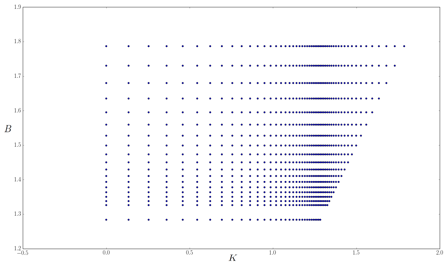
Figure 3.1: Hyperbolic mesh on the domain $\{(K,B):0<K\vee S_{0}<B\}$, initialised with “blank layers”.

In order to perform numerical tests, we calibrate a pure local volatility model to the set of vanilla options presented in Section 2.1 and obtain a local volatility function $\sigma_{\rm LV}$. Our implementation follows a fixed-point algorithm as described in [11] based on the work of [39]. Other methods to retrieve the local volatility function could have been used as well. From this calibrated local volatility we define a hypothetical volatility function of the form

$$\sigma\mathopen{}\mathclose{{}\left(s,m,t}\right)=\sqrt{\sigma_{\rm LV}\mathopen{}\mathclose{{}\left(s,t}\right)\sigma_{\rm LV}\mathopen{}\mathclose{{}\left(m,t}\right)}\qquad m\geq s\,,$$

defined on a mesh of strikes, barriers and maturities $\mathopen{}\mathclose{{}\left(K_{T_{i},j},B_{T_{i},k},T_{i}}\right)$, with $1\leq i\leq 10$ , $1\leq j\leq 5$ and $1\leq k\leq 5$ such that $B_{T_{i,},k}=K_{T_{i},k}$ and interpolated with cubic splines in space and constant backwards in time. The initial spot value is $S_{0}=1.2837$.

For a smooth transition at the boundaries to a constant extrapolation, we propose a smooth transformation by a change of coordinates in Appendix A.4. We plot in Figure 3.6 the thus assumed volatility. We emphasise that this volatility surface is in itself not calibrated to any derivatives and used purely as a numerical test example for the discretisation scheme.

In order to demonstrate the importance of “blank layers”, we plot the value of (3.6) obtained with $N=700$ and $M=100$, as a function of $B$ for $T=1$ with and without “blank layers” in Figure 3.2 and 3.3 respectively. Evaluating the term $\phi(B,B,T)$ from (2) accurately is necessary since the value of the foreign no touch option is directly linked to it by

$$\frac{\partial C\mathopen{}\mathclose{{}\left(0,B,T}\right)}{\partial T}+r^{\rm f}\!\!\!\!\;\;(T)C\mathopen{}\mathclose{{}\left(0,B,T}\right)=-\frac{1}{2}\sigma^{2}\mathopen{}\mathclose{{}\left(B,B,T}\right)B^{3}\phi\mathopen{}\mathclose{{}\left(B,B,T}\right)\qquad\forall\mathopen{}\mathclose{{}\left(B,T}\right)\in\mathopen{}\mathclose{{}\left(S_{0},+\infty}\right)\times\mathbb{R}_{*}^{+}.$$

Finally, to highlight the importance of a smoothing scheme for the time stepping, we plot $\phi(B,B,T)$ with “blank layers” combined with BDF2 in Figure 3.4 and Crank–Nicolson in Figure 3.5, which shows that Crank–Nicolson can generate instabilities if the number of time steps is too small, even when using Rannacher initialisation.

?figurename? 3.2: $\partial^{3}C/\partial K^{2}\partial B$ along the diagonal $K=B$ for $T=1$, initialised with “blank layers". 700 strike steps, 100 BDF2 time steps + Rannacher initialisation.

?figurename? 3.3: $\partial^{3}C/\partial K^{2}\partial B$ along the diagonal $K=B$ for $T=1$, initialised without “blank layers". 700 strike steps, 100 BDF2 time steps + Rannacher initialisation.

?figurename? 3.4: $\partial^{3}C/\partial K^{2}\partial B$ along the diagonal, for $T=1$, initialised with “blank layers". 700 strike steps, 10 BDF2 time steps + Rannacher initialisation.

?figurename? 3.5: $\partial^{3}C/\partial K^{2}\partial B$ along the diagonal for $T=1$, initialised with “blank layers". 700 strike steps, 10 Crank–Nicolson time steps + Rannacher initialisation.

In order to numerically verify the PIDE solution, we compute the price of an up-and-out call option for $K=80\%\times S_{0}$, $B=110\%\times S_{0}$ and $T=1$ with the forward PIDE and crude Monte Carlo combined with the Brownian bridge (BB) technique as in Chapter 6 of [18].

The results are shown in Table 3.1.

Forward PIDE	Monte Carlo (with 95% conf. int.)
0.15823	0.15825 (0.15821, 0.15828)

Table 3.1: Price of an up-and-out call option for $K=80\%\times S_{0}$, $B=110\%\times S_{0}$, computed with the forward PIDE (700 spot steps and 100 time steps) and Monte Carlo ($5\times 10^{7}$ paths and 500 time steps with Brownian bridge interpolation).

In Table 3.2, we give the convergence order as a function of the number of strike points. More precisely, the error $e_{n}$ in row $n$ is the absolute difference between the value with $2\times N_{K}$ and $N_{K}$ strike points, $N_{K}=150\times 2^{n}$. The order displayed in row $n$ is then $\ln\mathopen{}\mathclose{{}\left(e_{n}/e_{n+1}}\right)/\ln 2$. We notice that while the convergence order is close to $3$ for a smaller number of strike points, the asymptotic order is indeed 2. A similar approach is used for Table 3.3, where convergence of order 2 is obtained after 240 time steps per year. However, even for a smaller number of time steps, the error is small and the price is accurate.

$N_{K}$	Error	Order
300	$9.43\times 10^{-6}$	2.93
600	$1.38\times 10^{-6}$	2.03
1200	$3.23\times 10^{-7}$	1.98
2400	$6.53\times 10^{-8}$	–

Table 3.2: Convergence order in number of strike steps $N_{K}$ for $N_{T}=60$ time steps.

$N_{T}$	Error	Order
60	$7.58\times 10^{-6}$	1.12
120	$3.48\times 10^{-6}$	-0.99
240	$6.91\times 10^{-6}$	2.07
480	$1.64\times 10^{-6}$	2.04
960	$3.99\times 10^{-7}$	–

Table 3.3: Convergence order in number of time steps $N_{T}$ for $N_{K}=1200$ strike steps.

We re-iterate the non-standard nature of the PIDE and that it was only by a careful adaptation of standard techniques that high accuracy and stability was achieved.

Finally, we show in Figure 3.7 up-and-out call prices for $T=1$ as a function of $K$ and $B$ where we have $S_{0}=1.2837$.

?figurename? 3.6: Volatility function used for numerical test with smooth transition at the boundary. The construction is such that $\sigma\mathopen{}\mathclose{{}\left(s,m,t}\right)=\sqrt{\sigma_{\mathrm{LV}}\mathopen{}\mathclose{{}\left(s,t}\right)\sigma_{\mathrm{LV}}\mathopen{}\mathclose{{}\left(m,t}\right)}$.

Figure 3.7: Up-and-out call prices computed with the forward PIDE for different values of strikes and barriers and $T=1$.

4 Calibration of path-dependent volatility models

For the calibration to options with barrier features, whose payoff thus depends on the running maximum of the underlying asset, it seems natural to also consider models where the volatility depends explicitly on the maximum. This leads to models from the class of path-dependent volatility models proposed in [21].

To this end, let the range of possible $(S_{t},M_{t})$ values be

$${\mathcal{D}}=\mathopen{}\mathclose{{}\left\{\mathopen{}\mathclose{{}\left(s,m}\right)\in\mathbb{R}^{2}:\,0\leq s\vee S_{0}\leq m}\right\}\,.$$

First, we define a “local maximum volatility” (LMV) model by

$$\begin{cases}\cfrac{dS_{t}}{S_{t}}=\mathopen{}\mathclose{{}\left(r^{\rm d}\!\!\!\!\;\;(t)-r^{\rm f}\!\!\!\!\;\;(t)}\right)\,dt+\sigma_{\mathrm{LMV}}\mathopen{}\mathclose{{}\left(S_{t},M_{t},t}\right)\,dW_{t}\\ M_{t}=\underset{0\leq u\leq t}{\max}S_{u}\,,\end{cases}$$ (4.1)

where $\sigma_{\mathrm{LMV}}\,:\,{\mathcal{D}}\times\mathopen{}\mathclose{{}\left[0,T}\right]\rightarrow\mathbb{R}^{+}$ is assumed to be bounded, locally Lipschitz in $S$ and continuously differentiable in $M$. This implies that $(S_{t},M_{t})_{t\geq 0}$ is Markovian (see [6]). The construction is motivated by the ability of the model to mimick the joint distribution of $S_{t}$ and $M_{t}$ for any diffusion model, as shown in [6], and therefore it can fit up-barrier option prices simultaneously for all maturities, strikes, and barrier levels by construction.

Secondly, we propose a “local maximum stochastic volatility” (LMSV) model defined as

$$\begin{array}[]{c}\begin{cases}\cfrac{dS_{t}}{S_{t}}=\mathopen{}\mathclose{{}\left(r^{\rm d}\!\!\!\!\;\;(t)-r^{\rm f}\!\!\!\!\;\;(t)}\right)\,dt+\sigma\mathopen{}\mathclose{{}\left(S_{t},M_{t},t}\right)\sqrt{V_{t}}\,dW_{t}\\ dV_{t}=\kappa\mathopen{}\mathclose{{}\left(\theta-V_{t}}\right)\,dt+\xi\sqrt{V_{t}}\,dW_{t}^{V}\\ M_{t}=\underset{0\leq u\leq t}{\max}S_{u}\,,\end{cases}\end{array}$$ (4.2)

with $\sigma:\,{\mathcal{D}}\times\mathopen{}\mathclose{{}\left[0,T}\right]\rightarrow\mathbb{R}^{+}$ a local volatility function which also depends on the running maximum. This model extends (4.1) in the same way that the LSV model extends the LV model. One might also wish to incorporate a mixing factor $\beta$ as in (2.4). This would fit naturally into the calibration proposed below.

Note that the class of models in (2.1) includes (4.1) and (4.2).

In the following, we discuss the calibration of the path-dependent volatility model (4.1) by forward PIDE (2) to vanilla and no-touch options.

4.1 LMV model calibration with regularised best-fit algorithm

As the LMV model represents the natural extension of the Dupire local volatility model for European calls to up-and-out barriers, the approach taken here is motivated by the literature on calibration and regularisation of local volatility. Our goal is to encode the market prices of both vanilla options and no-touches in one model. Moreover, it represents a building block to the calibration of the LMSV model in Section 4.3 by particle method.

The local maximum volatility function $\sigma_{\mathrm{LMV}}$ is calibrated directly to these quotes and cannot be expected to be unique, as the marginal distributions of $S$ (from the vanillas) and $M$ (from the no-touches) do not uniquely identify their joint distribution. How much they restrict the joint distribution is an interesting reseach question.

Specifically, we will minimise a functional consisting of the least-squares model error for vanillas and no-touches and a penalty term which steers the optimisation algorithm to a local minimum with certain regularity. The optimisation is performed over volatility surfaces which are parameterised with a finite dimensional parameter vector $\Lambda_{i}$ for each $(T_{i-1},T_{i})$.

In our tests, the volatility function is defined by quadratic splines in spot and running maximum and piecewise constant in time. For each quoted maturity, we choose a grid of points formed by the $N_{K}=5$ quoted strikes in the spot direction and $N_{B}=4$ nodes $\mathopen{}\mathclose{{}\left(M_{T_{i},k}}\right)_{1\leq k\leq N_{B}}$ in the running maximum direction, uniformly spaced on the interval

$$\mathopen{}\mathclose{{}\left[S_{0}+\frac{\mathopen{}\mathclose{{}\left(B_{T_{i},50\%}-S_{0}}\right)}{4},\,B_{T_{i},90\%}}\right],$$

where $B_{T_{i},50\%}$ and $B_{T_{i},90\%}$ are, respectively, the quoted up-and-out barriers for the corresponding $50\%$ and $90\%$ no-touch probabilities for maturity $T_{i}$. The optimisation will be performed over the $\mathopen{}\mathclose{{}\left(N_{K}\times N_{B}}\right)$ matrix

$$\Lambda_{i}\mathbf{=}\mathopen{}\mathclose{{}\left[\sigma_{\mathrm{LMV}}^{i,j,k}}\right]_{j,k},$$

with $\sigma_{\mathrm{LMV}}^{i,j,k}=\sigma_{\mathrm{LMV}}\mathopen{}\mathclose{{}\left(K_{T_{i},j},M_{T_{i},k},T_{i}}\right)$, with $1\leq i\leq N_{\text{Mat}}$, $1\leq j\leq N_{K}$, $1\leq k\leq N_{B}$. For a given maturity $T_{i}$, the volatility is extrapolated asymptotically constant as described in Appendix A.4, outside $\mathopen{}\mathclose{{}\left[K_{T_{i},1},K_{T_{i},N_{K}}}\right]\times\mathopen{}\mathclose{{}\left[M_{T_{i},1},K_{T_{i},N_{B}}}\right]$.

We define the objective function $\bar{e}$ for $Q_{K}$ quoted strikes, $Q_{B}$ quoted barrier levels and each maturity $T_{i}$ as

$$\bar{e}\mathopen{}\mathclose{{}\left(\Lambda_{i}}\right) = e\mathopen{}\mathclose{{}\left(\Lambda_{i}}\right)\mathopen{}\mathclose{{}\left(1+\mathcal{P}\mathopen{}\mathclose{{}\left(\Lambda_{i}}\right)}\right)$$

$$e\mathopen{}\mathclose{{}\left(\Lambda_{i}}\right) = \sum_{l=1}^{Q_{B}}\mathopen{}\mathclose{{}\left(e_{l}^{\mathrm{FNT}}\mathopen{}\mathclose{{}\left(\Lambda_{i}}\right)}\right)^{2}+\gamma^{2}\sum_{l=1}^{Q_{K}}\mathopen{}\mathclose{{}\left(e_{l}^{\Sigma}\mathopen{}\mathclose{{}\left(\Lambda_{i}}\right)}\right)^{2},$$

$$e_{l}^{\mathrm{FNT}}\mathopen{}\mathclose{{}\left(\Lambda_{i}}\right) = \mathrm{FNT}^{\text{Model}}\mathopen{}\mathclose{{}\left(B_{T_{i},l},T_{i},\Lambda_{i}}\right)-\mathrm{FNT}^{\text{Market}}\mathopen{}\mathclose{{}\left(B_{T_{i},l},T_{i}}\right)$$ (4.3)

$$e_{l}^{\Sigma}\mathopen{}\mathclose{{}\left(\Lambda_{i}}\right) = \Sigma^{\text{Model}}\mathopen{}\mathclose{{}\left(K_{T_{i},l},T_{i},\Lambda_{i}}\right)-\Sigma^{\text{Market}}\mathopen{}\mathclose{{}\left(K_{T_{i},l},T_{i}}\right)\,,$$ (4.4)

with $\Sigma^{\text{Market}}$ the market Black–Scholes implied volatility, $\Sigma^{\text{Model}}$ the model implied volatility, $\gamma\in\mathbb{R}$ and

$$\mathcal{P}\mathopen{}\mathclose{{}\left(\Lambda_{i}}\right) \!\!=\!\! \frac{1}{N_{K}N_{B}}\sum_{l=1}^{N_{K}}\sum_{m=1}^{N_{B}}\mathopen{}\mathclose{{}\left(\frac{\partial^{2}\sigma_{\mathrm{LMV}}\mathopen{}\mathclose{{}\left(K_{T_{i},l},M_{T_{i},m},T_{i}}\right)}{\partial K^{2}}}\right)^{2}h\mathopen{}\mathclose{{}\left(-\frac{\partial^{2}\sigma_{\mathrm{LMV}}\mathopen{}\mathclose{{}\left(K_{T_{i},l},M_{T_{i},m},T_{i}}\right)}{\partial K^{2}},0.5,0.5}\right)$$ (4.5)

$$h\mathopen{}\mathclose{{}\left(x,x_{0},\epsilon}\right) \!\!=\!\! \frac{1+\text{tanh}(2\frac{\mathopen{}\mathclose{{}\left(x-x_{0}}\right)}{\epsilon})}{2}\,,$$

where the second derivative is obtained by differentiation of the interpolant. Note that $\bar{e}$, $e$ and $\mathcal{P}$ at $T_{i}$ are functions of $\mathopen{}\mathclose{{}\left(\Lambda_{i}}\right)_{j\leq i}$, but in writing $e\mathopen{}\mathclose{{}\left(\Lambda_{i}}\right)$ etc, we focus on the dependence on $\Lambda_{i}$ for the inductive calibration.

The penalisation function $\mathcal{P}$ is a Tikhonov-type regularisation which reduces the number of local minima and improves the stability of the volatility surface. For a pure local volatility model, Tikhonov regularisation has been shown to provide well-posedness, under the condition that the local volatility does not depend on time, for the one maturity vanilla calibration problem in [14]. A similar approach is also used in [12] for the pure local volatility model. The parametric form (4.5) for the penalisation was chosen empirically. We acknowledge that the penalised error $\bar{e}\mathopen{}\mathclose{{}\left(\Lambda_{i}}\right)$ as defined in (4.1) does not prevent over-parametrisation if the market data fit perfectly, i.e. when $e\mathopen{}\mathclose{{}\left(\Lambda_{i}}\right)=0$, as the penalisation is multiplicative. However, during the iterative optimisation we found $e\mathopen{}\mathclose{{}\left(\Lambda_{i}}\right)$ to be always strictly positive and the penalisation will favour smoother, convex shapes of the volatility in the strike direction; see also Section 4.1. Here, $h$ acts as a smoothed step function to ensure differentiability with respect to the parameters $\Lambda_{i}$ (for the BFGS routine used below). Setting, $\epsilon=0.5\text{ and }x_{0}=0.5$, is such that we get $h\mathopen{}\mathclose{{}\left(0,0.5,0.5}\right)\approx 0.02$, a small positive amount in order to penalise mainly concave solutions while lightly penalising close-to linear solutions as well. In that sense, $h$ helps minimise the impact of small values of the second order derivative.

The calibration algorithm is described in Algorithm 1 in Appendix B for $N_{\text{Mat}}$ maturity pillars where we use the calibrated local volatility (i.e., $\sigma_{\mathrm{LMV}}(S_{t},M_{t},t)=\sigma_{\mathrm{LV}}(S_{t},t)$ independent of $M_{t}$) as a first guess for the first maturity pillar.

The calibration algorithm uses the bounded L-BFGS routine described in [42], where the gradient of the objective function $\bar{e}$ needs to be computed. Compared to the gradient-free Nelder–Mead [32] algorithm discussed in Section 5, the L-BFGS optimisation is considerably faster to converge to a local-minimum if a gradient can be obtained efficiently. For instance, for parameter $\sigma_{\mathrm{LMV}}^{i,j,k}$, we can write

$$\frac{\partial e\mathopen{}\mathclose{{}\left(\Lambda_{i}}\right)}{\partial\sigma_{\mathrm{LMV}}^{i,j,k}} = 2\sum_{l=1}^{Q_{B}}e_{l}^{\mathrm{FNT}}\mathopen{}\mathclose{{}\left(\Lambda_{i}}\right)\frac{\partial\mathrm{FNT}^{\text{Model}}\mathopen{}\mathclose{{}\left(T_{i},B_{T_{i},l},\Lambda_{i}}\right)}{\partial\sigma_{\mathrm{LMV}}^{i,j,k}}+2\gamma^{2}\sum_{l=1}^{Q_{K}}\frac{e_{l}^{\Sigma}\mathopen{}\mathclose{{}\left(\Lambda_{i}}\right)}{\mathcal{V}\mathopen{}\mathclose{{}\left(T_{i},K_{T_{i},l},\sigma_{\mathrm{LMV}}^{i,j,k}}\right)}\frac{\partial{\rm Call}{}^{\text{Model}}\mathopen{}\mathclose{{}\left(T_{i},K_{T_{i},l},\Lambda_{i}}\right)}{\partial\sigma_{\mathrm{LMV}}^{i,j,k}},$$

where $\mathcal{V}\mathopen{}\mathclose{{}\left(T,K,\sigma}\right)$ is the standard Black–Scholes vega for maturity $T$, strike $K$ and volatility $\sigma$. The computation of the gradient of the model up-and-out call price $C\mathopen{}\mathclose{{}\left(K,B,T,\Lambda_{i}}\right)$ (including calls and no-touches) with respect to the parameter vector $\Lambda_{i}$ is described in Section 4.2.

The model prices were computed using the PIDE (2) discretised with $1200$ strike steps, $40$ time steps in between each quoted maturity $T_{i}$, which is sufficient to guarantee good accuracy.

In order to emphasise the importance of the penalisation function, we calibrate the LMV model without regularisation, i.e. $\mathcal{P}\equiv 0$, and plot the resulting LMV function in Figures 4.3 and 4.4, with the same axis range as for the regularised solution in Figures 4.1 and 4.2, which highlights different possible solutions, especially for longer maturities. We used $\gamma=5$ in (4.1).

The calibration process shows the existence of a few local minima in the objective function. This is not surprising as the path-dependent volatility model is, in principle, able to calibrate perfectly a discrete set of up-and-out call options (which includes vanilla options), hence by only providing call and no-touch prices, the calibration problem is underdetermined.

In the present setting, with five vanilla and five no-touch quotes per maturity, and 20 parameters, we find many surfaces which fit the data. However, starting the iterative optimisation procedure from the Dupire volatility (i.e., no dependence on the maximum), the regularisation steers the approximate minimiser towards a calibrated surface with small penalty term.

?figurename? 4.1: Local maximum volatility function $T=1Y$ with regularisation.

?figurename? 4.2: Local maximum volatility function $T=5Y$ with regularisation.

?figurename? 4.3: Local maximum volatility function $T=1Y$ with no regularisation.

?figurename? 4.4: Local maximum volatility function $T=5Y$ with no regularisation.

We will see in Section 6, specifically the first column of Table 6.2, that the calibration is very precise, with an absolute error for no-touches never higher than $0.03\%$ in price.

4.2 Gradient operator with respect to the volatility parameters

In order to perform a best-fit algorithm, knowledge of the gradient with respect to the model parameters is required for the chosen (gradient-based) optimisation process. Assume that the volatility in $(T_{i},T_{i+1})$ is a function of $N$ parameters $\Lambda_{i}=\mathopen{}\mathclose{{}\left(\sigma_{i,1},...,\sigma_{i,N}}\right)$, and constant between quoted maturities, where we drop the subscript ‘LMV’ for brevity.

So, we need to compute $\nabla C\mathopen{}\mathclose{{}\left(\sigma_{i,1},...,\sigma_{i,N}}\right),$ where $\nabla$ is the gradient operator with respect to $\Lambda_{i}$.

Equation (2) can be written as

$$\frac{\partial C\mathopen{}\mathclose{{}\left(\Lambda_{i}}\right)}{\partial T}+r^{\rm f}\!\!\!\!\;\;(T)C\mathopen{}\mathclose{{}\left(\Lambda_{i}}\right)+\mathopen{}\mathclose{{}\left(r^{\rm d}\!\!\!\!\;\;(T)-r^{\rm f}\!\!\!\!\;\;(T)}\right)K\frac{\partial C\mathopen{}\mathclose{{}\left(\Lambda_{i}}\right)}{\partial K}-\frac{1}{2}\sigma^{2}\mathopen{}\mathclose{{}\left(\Lambda_{i}}\right)K^{2}\frac{\partial^{2}C\mathopen{}\mathclose{{}\left(\Lambda_{i}}\right)}{\partial K^{2}}=\hskip 99.58464pt$$

$$-\frac{1}{2}\mathopen{}\mathclose{{}\left.\sigma^{2}\mathopen{}\mathclose{{}\left(\Lambda_{i}}\right)}\right\rfloor_{K=B}B^{2}\mathopen{}\mathclose{{}\left(B-K}\right)\mathopen{}\mathclose{{}\left.\frac{\partial^{3}C\mathopen{}\mathclose{{}\left(\Lambda_{i}}\right)}{\partial K^{2}\partial B}}\right\rfloor_{K=B}-\int_{S_{0}\lor K}^{B}K^{2}\frac{\partial^{2}C\mathopen{}\mathclose{{}\left(\Lambda_{i}}\right)}{\partial K^{2}}\sigma\mathopen{}\mathclose{{}\left(\Lambda_{i}}\right)\frac{\partial\sigma\mathopen{}\mathclose{{}\left(\Lambda_{i}}\right)}{\partial b}\,{\,\rm d}b\,.$$

We can differentiate with respect to each of the parameter vectors $\Lambda_{i}$, which gives

$$\hskip 14.22636pt\frac{\partial\nabla C\mathopen{}\mathclose{{}\left(\Lambda_{i}}\right)}{\partial T}+r^{\rm f}\!\!\!\!\;\;(T)\nabla C\mathopen{}\mathclose{{}\left(\Lambda_{i}}\right)+\mathopen{}\mathclose{{}\left(r^{\rm d}\!\!\!\!\;\;(T)-r^{\rm f}\!\!\!\!\;\;(T)}\right)K\frac{\partial\nabla C\mathopen{}\mathclose{{}\left(\Lambda_{i}}\right)}{\partial K}-\frac{1}{2}\sigma^{2}\mathopen{}\mathclose{{}\left(\Lambda_{i}}\right)K^{2}\frac{\partial^{2}\nabla C\mathopen{}\mathclose{{}\left(\Lambda_{i}}\right)}{\partial K^{2}}=\hskip 99.58464pt$$

$$-\frac{1}{2}\mathopen{}\mathclose{{}\left.\sigma^{2}\mathopen{}\mathclose{{}\left(\Lambda_{i}}\right)}\right\rfloor_{K=B}B^{2}\mathopen{}\mathclose{{}\left(B-K}\right)\mathopen{}\mathclose{{}\left.\frac{\partial^{3}\nabla C\mathopen{}\mathclose{{}\left(\Lambda_{i}}\right)}{\partial K^{2}\partial B}}\right\rfloor_{K=B}-\int_{S_{0}\lor K}^{B}K^{2}\frac{\partial^{2}\nabla C\mathopen{}\mathclose{{}\left(\Lambda_{i}}\right)}{\partial K^{2}}\sigma\mathopen{}\mathclose{{}\left(\Lambda_{i}}\right)\frac{\partial\sigma\mathopen{}\mathclose{{}\left(\Lambda_{i}}\right)}{\partial b}\,{\,\rm d}b+R\mathopen{}\mathclose{{}\left(\Lambda_{i}}\right)\,,$$

with

$$R\mathopen{}\mathclose{{}\left(\Lambda_{i}}\right) = \sigma\mathopen{}\mathclose{{}\left(\Lambda_{i}}\right)\mathopen{}\mathclose{{}\left(\nabla\sigma\mathopen{}\mathclose{{}\left(\Lambda_{i}}\right)}\right)K^{2}\frac{\partial^{2}C\mathopen{}\mathclose{{}\left(\Lambda_{i}}\right)}{\partial K^{2}}-\mathopen{}\mathclose{{}\left.\mathopen{}\mathclose{{}\left(\sigma\mathopen{}\mathclose{{}\left(\Lambda_{i}}\right)\mathopen{}\mathclose{{}\left(\nabla\sigma\mathopen{}\mathclose{{}\left(\Lambda_{i}}\right)}\right)}\right)}\right\rfloor_{K=B}B^{2}\mathopen{}\mathclose{{}\left(B-K}\right)\mathopen{}\mathclose{{}\left.\frac{\partial^{3}C\mathopen{}\mathclose{{}\left(\Lambda_{i}}\right)}{\partial K^{2}\partial B}}\right\rfloor_{K=B}$$

$$-\int_{S_{0}\lor K}^{B}K^{2}\frac{\partial^{2}C\mathopen{}\mathclose{{}\left(\Lambda_{i}}\right)}{\partial K^{2}}\mathopen{}\mathclose{{}\left(\nabla\mathopen{}\mathclose{{}\left(\sigma\mathopen{}\mathclose{{}\left(\Lambda_{i}}\right)}\right)\frac{\partial\sigma\mathopen{}\mathclose{{}\left(\Lambda_{i}}\right)}{\partial b}+\sigma\mathopen{}\mathclose{{}\left(\Lambda_{i}}\right)\nabla\mathopen{}\mathclose{{}\left(\frac{\partial\sigma\mathopen{}\mathclose{{}\left(\Lambda_{i}}\right)}{\partial b}}\right)}\right)\,{\,\rm d}b\,.$$

Hence, $\nabla C\mathopen{}\mathclose{{}\left(\Lambda_{i}}\right)$ follows the same PDE as $C$, but with an inhomogeneous term which is a function of $C$ and its spatial derivatives, with initial condition

$$\nabla C\mathopen{}\mathclose{{}\left(\Lambda_{i}}\right)\mathopen{}\mathclose{{}\left(K,B,0}\right)=0\qquad 0\leq K,\quad K\vee S_{0}\leq B,$$

and with boundary conditions

$$\nabla C\mathopen{}\mathclose{{}\left(\Lambda_{i}}\right)\mathopen{}\mathclose{{}\left(B,B,T}\right)=0, S_{0}\leq B,$$

$$\nabla C\mathopen{}\mathclose{{}\left(\Lambda_{i}}\right)\mathopen{}\mathclose{{}\left(K,S_{0},T}\right)=0, K\leq S_{0},$$

which match the Dirichlet boundary conditions for $C\mathopen{}\mathclose{{}\left(K,B,T}\right)$. This useful property confirms that we can use the same discretised linear operator for both $C$ and $\nabla C\mathopen{}\mathclose{{}\left(\Lambda_{i}}\right)$. The additional source term $R$ on the right-hand side is fully known since the solution for $C$ is computed beforehand. Only one costly LU factorisation is needed to compute both $C$ and $\nabla C\mathopen{}\mathclose{{}\left(\Lambda_{i}}\right)$ at each implicit time step. Solving the linear systems of $N+1$ equations is then fast by forward and backward substitution. Additionally, since the volatility is assumed piecewise constant in maturity, the set of parameters $\Lambda_{i+1}$ has no impact on the values of $C\mathopen{}\mathclose{{}\left(K,B,T}\right)$ for any $T\leq T_{i}$. Hence we also have

$$\nabla C\mathopen{}\mathclose{{}\left(\Lambda_{i}}\right)\mathopen{}\mathclose{{}\left(K,B,T_{j}}\right)=0,\,j<i\,.$$

Some numerical experiments for a volatility defined on a grid of $5\times 5$ points, i.e. $25$ parameters, showed that the additional evaluation of the gradient (with respect to each of the parameters) requires only twice the time needed to solve the PDE. As a comparison, the powerful adjoint algorithmic differentiation (AAD) technique (see [17] for applications in derivative pricing) can achieve the same task for a computational time between three to four times the time needed to solve the original PDE independent of the number of parameters (see Section 4.6 in [19]). Therefore, the chosen approach leads to a competitive computational time in the present setting. The gradient components can be computed in parallel which would further reduce the computational cost.

4.3 Calibration of the LMSV model by 2D particle method

In this section, we discuss a possible calibration algorithm for the LMSV model (4.2). We assume that a calibrated LMV volatility function $\sigma_{\mathrm{LMV}}$ is at our disposal, e.g. obtained as in Section 4.1.

With the Heston parameters $(\kappa,\xi,\theta)$ and $\sigma_{\mathrm{LMV}}$ fixed, $\sigma$ in (4.2) can be found from the calibration condition (see (2.9) and thereafter)

$$\sigma^{2}(K,B,T)\,\mathbb{E}^{\mathbb{Q}^{\rm d}}\mathopen{}\mathclose{{}\left[V_{T}^{2}\,|\,S_{T}=K,\,M_{T}=B}\right] = \sigma_{\mathrm{LMV}}^{2}\mathopen{}\mathclose{{}\left(K,B,T}\right)\,.$$ (4.6)

Through the conditional expectation, the function $\sigma$ in (4.6) depends on the distribution of the joint process $X=(X_{t})_{t\geq 0}=\mathopen{}\mathclose{{}\left(S_{t},M_{t},V_{t}}\right)_{t\geq 0}$. If we insert $\sigma$ expressed from (4.6) in (4.2) for a model calibrated to vanilla and barrier quotes, via $\sigma_{\mathrm{LMV}}$, the resulting process thus falls in the class of McKean-Vlasov processes [30].

The particle method for the estimation of conditional expectations was introduced in [30], and is discussed in detail in [38]; it was applied to LSV model calibration in [22, 23]. More details about stochastic filtering problems, as well as a literature review, can also be found in [4].

We consider $N$-sample paths $\mathopen{}\mathclose{{}\left(X_{t}^{i}}\right)_{1\leq i\leq N}=\mathopen{}\mathclose{{}\left(S_{t}^{i},M_{t}^{i},V_{t}^{i}}\right)_{1\leq i\leq N}$, $t\geq 0$, i.e. $N$ independent realisations of $X$, and write for brevity ${\bf X}_{\cdot}=\mathopen{}\mathclose{{}\left(X_{\cdot}^{i}}\right)_{1\leq i\leq N}$.

The ($3\times N$)-dimensional SDE driving the system ${\bf X}$ in the case of the LMSV model can be approximated by

$$\begin{cases}\cfrac{d\hat{S}_{t}^{i}}{\hat{S}_{t}^{i}}=\mathopen{}\mathclose{{}\left(r^{\rm d}\!\!\!\!\;\;(t)-r^{\rm f}\!\!\!\!\;\;(t)}\right)\,dt+\hat{\sigma}_{N}\!\mathopen{}\mathclose{{}\left(\hat{S}_{t}^{i},\hat{M}_{t}^{i},t;{\bf X}}\right)\sqrt{V_{t}^{i}}\,dW_{t}^{i}\\ dV_{t}^{i}=\kappa\mathopen{}\mathclose{{}\left(\theta-V_{t}^{i}}\right)\,dt+\xi\sqrt{V_{t}^{i}}\,dW_{t}^{V,i}\\ \hat{M}_{t}^{i}=\underset{0\leq u\leq t}{\max}\hat{S}_{u}^{i}\,,\end{cases}$$

where $(W_{\cdot}^{i},W_{\cdot}^{V,i})$, $1\leq i\leq N$, are independent samples of the two correlated driving Brownian motions, $\hat{\sigma}_{N}$ is an estimator for $\sigma$ to be defined below, and $\hat{{\bf X}}_{t}=\mathopen{}\mathclose{{}\left(\hat{X}_{t}^{i}}\right)_{1\leq i\leq N}=\mathopen{}\mathclose{{}\left(\hat{S}_{t}^{i},\hat{M}_{t}^{i},V_{t}^{i}}\right)_{1\leq i\leq N}$, $t\geq 0$, with $\hat{M}_{t}^{i}=\sup_{s\leq t}\hat{S}_{t}^{i}$.

We use an extension of the QE-scheme [1] (see also Section 5.1) where the volatility now depends on the running maximum as well as the spot. The Brownian increments are generated with a pseudorandom number generator.s The running maximum is sampled approximately with a Brownian bridge technique as described in Chapter 6 of [18], with $\sigma$ kept constant in time between timesteps,

$$G_{t} = \frac{S_{t}+S_{t+\Delta t}+\sqrt{\mathopen{}\mathclose{{}\left(S_{t}+S_{t+\Delta t}}\right)^{2}-2\mathopen{}\mathclose{{}\left(S_{t}\sigma\mathopen{}\mathclose{{}\left(S_{t},t}\right)\sqrt{V_{t}}}\right)^{2}\,\Delta t\,\log\mathopen{}\mathclose{{}\left(U_{t}}\right)}}{2}$$

$$M_{t+\Delta t} = \max\mathopen{}\mathclose{{}\left(G_{t},M_{t}}\right)\,,$$

where $U_{t}$ is an independent draw from the uniform distribution $\mathcal{U}\mathopen{}\mathclose{{}\left(0,1}\right)$, i.i.d. across $t$.

The accuracy of the integration of the SDE would be of lesser importance if the same scheme were used in calibration and pricing, since the calibration will be to the conditional law of the (approximate) model. Here, we discuss calibration by PIDE and pricing by MC and hence use an accurate timestepping scheme.

We refer to [22] and [38] for more extensive details about the particle method and conditions for its convergence (which, to the best of our knowledge, are not proven for the present case).

For the construction of the LMSV by particle method, we estimate the Markovian projection (2.9) as

$$\hat{p}_{N}\mathopen{}\mathclose{{}\left(K,B,T;{\bf X}_{T}}\right)=\frac{\frac{1}{N}\sum_{i=1}^{N}V_{T}^{i}\delta_{N}\mathopen{}\mathclose{{}\left(S_{T}^{i}-K,\,M_{T}^{i}-B,T}\right)+2\theta\xi\epsilon}{\frac{1}{N}\sum_{i=1}^{N}\delta_{N}\mathopen{}\mathclose{{}\left(S_{T}^{i}-K,\,M_{T}^{i}-B,T}\right)+\xi\epsilon},$$ (4.7)

with $\delta_{N}$ an anisotropic bi-variate Gaussian kernel

$$\delta_{N}\mathopen{}\mathclose{{}\left(x,y,T}\right) = \frac{\text{exp}\mathopen{}\mathclose{{}\left(-\frac{1}{2}\frac{\zeta\mathopen{}\mathclose{{}\left(T}\right)}{1-\rho_{xy}^{2}\mathopen{}\mathclose{{}\left(T}\right)}}\right)}{\gamma\mathopen{}\mathclose{{}\left(T}\right)}\,$$ (4.8)

$$\zeta\mathopen{}\mathclose{{}\left(T}\right) = \frac{x^{2}}{h_{x}^{2}\mathopen{}\mathclose{{}\left(T}\right)}+\frac{y^{2}}{h_{y}^{2}\mathopen{}\mathclose{{}\left(T}\right)}-2\frac{\rho_{xy}\mathopen{}\mathclose{{}\left(T}\right)xy}{h_{x}\mathopen{}\mathclose{{}\left(T}\right)h_{y}\mathopen{}\mathclose{{}\left(T}\right)}$$

$$\gamma\mathopen{}\mathclose{{}\left(T}\right) = 2\pi h_{x}\mathopen{}\mathclose{{}\left(T}\right)h_{y}\mathopen{}\mathclose{{}\left(T}\right)\sqrt{1-\rho_{xy}^{2}\mathopen{}\mathclose{{}\left(T}\right)}\,,$$

where $h_{x}$, $h_{y}$, $\rho_{xy}$ as well as the specific bandwidth details are again given in Appendix A.1. When we used the normal Silverman rule bandwidth with $\rho_{xy}\mathopen{}\mathclose{{}\left(T}\right)=0$, the accuracy was found to drop drastically and became unsatisfactory for the considered number of particles in the range $100\,000-2\,000\,000$. We note that cheaper to evaluate kernels, such as uniform or triangle kernels, could be considered for better performance. Additionally, we used a high number of particles for our numerical study, however, a smaller sample size will likely suffice for most calibrations.

The extra terms $2\theta\xi\epsilon$ and $\xi\epsilon$ in (4.7) serve as a smooth extrapolation rule for areas containing only a few particles. for all $t$, then the calibration algorithm recovers, as expected, the calibrated path-dependent (mimicking) volatility $\sigma_{\mathrm{LMV}}$. Similarly, if $\xi=0$, then $V$ is deterministic and a single particle is sufficient to calibrate the LMSV model.

Then, $\sigma$ can be estimated by

$$\hat{\sigma}_{N}\mathopen{}\mathclose{{}\left(K,B,T;{\bf X}}\right)=\sqrt{\frac{\sigma_{\mathrm{LMV}}^{2}\mathopen{}\mathclose{{}\left(K,B,T}\right)}{\hat{p}_{N}\mathopen{}\mathclose{{}\left(K,B,T;{\bf X}}\right)}}\,,$$

with $\hat{p}_{N}\mathopen{}\mathclose{{}\left(K,B,T;{\bf X}}\right)$ given in (4.7) and ${{\bf X}}_{\cdot}=({S}^{i}_{\cdot},V^{i}_{\cdot},{M}^{i}_{\cdot})_{1\leq i\leq N}$.

The step-by-step calibration is detailed in Algorithm 2 in Appendix B.

The computational complexity of a direct evaluation of $\sigma_{\text{LMV}}$ by $\hat{p}_{N}\mathopen{}\mathclose{{}\left(S_{t}^{i},M_{t}^{i},t;{\bf X}_{t}}\right)$ for all particles is quadratic in $N$. To reduce the cost, we first approximate $\sigma_{\text{LMV}}$ on a mesh in $(S,M)$ and then interpolate by splines for the actual evaluation; see Appendix A.3 for details. We do not use any regularisation for $\sigma$ here.

Moreover, for a given point $(K,B)$ in (4.7), only a small number of particles in the vicinity contributes significantly to the sum due to the fast decay of the kernel function. We perform an efficient search for those particles on a $k$-d tree as described in Appendix A.1, which reduces the complexity per time step from $\mathcal{O}(N^{2})$ to $\mathcal{O}(N_{S}N_{M}\log N)$, if the 2D spline has $N_{S}N_{M}$ nodes.

Finally, we note that alternative approaches could be used in order to estimate the conditional expectation. One example would be to bucket the particles and then locally linearly regress on the variables, e.g., $S$ and $M$. This bucketing approach is used frequently for applications such as Monte Carlo valuation of American options and for CVA computations, to avoid having to use higher order polynomial terms as in the Longstaff–Schwartz algorithm [29].

We calibrated the model to the vanilla and no-touch quotes from Section 2.1. We plot in Figure 4.6 the calibrated local volatility function for $T=1$ with 350 time steps per year and $2\,000\,000$ particles. The calibration fit is compared to other models in Section 6.

?figurename? 4.5: Joint density $\phi\mathopen{}\mathclose{{}\left(S,M,T}\right)$ of the spot and running maximum after calibration at time $T=1$.

Figure 4.6: Calibrated local volatility function $\sigma\mathopen{}\mathclose{{}\left(S,M,T}\right)$ for the LMSV model at time $T=1$.

5 Calibration of the Heston-type LSV-LVV model

In this section, we describe the calibration of the LSV-LVV model (2.5) to both vanilla and no-touch options. Model (2.5) generalises the Heston-type LSV model (2.4) and we briefly discuss the prevalent approach to the calibration of this model first.

The calibration can be based on two different methods. On the one hand, if prices of exotic products are computed by Monte Carlo, it is possible to rely on a full Monte Carlo calibration approach. Accurate re-pricing of vanilla options will be ensured by computation of the particle estimator (5.2), while keeping track of the running maximum for each particle will allow to compute no-touch prices for all maturities and barrier levels. An optimisation algorithm can then be used to calibrate no-touch options. However, this approach leads to inaccuracies and parameter instabilities for longer maturities and higher barrier levels. Therefore, if one wishes to use PDE techniques in order to price a set of derivative products, a full Monte Carlo calibration becomes far less suitable. On the other hand, and in order to provide consistent and stable calibration for both PDE and Monte Carlo pricing, we propose a calibration method where no-touch prices are computed with PIDE (2), coupled with the LMV volatility calculated by a particle estimator we describe hereafter. This PIDE based calibration approach is described in the remainder of this section.

For any set of parameters $v_{0},\kappa,\theta,\xi,\rho$ in the Heston-LSV model ($\beta=1$), a sufficient condition on the local volatility function $\sigma$ (see, e.g., [23]) such that the model gives a perfect fit to arbitrage-free vanilla quotes is

$$\sigma\mathopen{}\mathclose{{}\left(K,T}\right) = \frac{\sigma_{\mathrm{LV}}\mathopen{}\mathclose{{}\left(K,T}\right)}{\sqrt{\mathbb{E}^{\mathbb{Q}^{\rm d}}\mathopen{}\mathclose{{}\left[V_{T}\,|\,S_{T}=K}\right]}}\,,$$ (5.1)

where $\sigma_{\mathrm{LV}}$ is a local volatility function (i.e., calibrated to vanilla quotes). Notice here that the right-hand side depends on $\sigma(\cdot,t)$ for $t<T$ through the conditional expectation.

One approach to the calibration is to consider the case $\sigma(S_{t},t)=1$ independent of $S_{t}$ and $t$ and calibrate a Heston type model with $\beta=1$ to the vanilla quotes by choice of $v_{0},\theta,\xi,\kappa,\rho$. Then, having established this choice of these parameters, $\beta$ is adjusted and for each choice the local volatility $\sigma(S,t)$ is recalibrated. The choice of $\beta$ is made for the best match to the barrier option prices (while by construction maintaining the calibration to the vanilla options).

The parameter $\beta$ is commonly within the range $[0,1]$ and called the “mixing factor” (see [10]): the market is believed to stand in between pure local volatility models, i.e. $\beta=0$, and full Heston LSV models, i.e. $\beta=1$. We show calibration results which support this claim in Section 6.

To improve the calibration accuracy to no-touch options, whose payoff depends on the running maximum, the vol-of-vol “local volatility function” is made spot- and time-dependent in our model (2.5).

5.1 Particle method and parametrisation of $\boldsymbol{\sigma}$

We satisfy the calibration condition (5.1) by a modificaiton of the particle method from Section 4.3.

We consider $N$-sample paths $\mathopen{}\mathclose{{}\left(X_{t}^{i}}\right)_{1\leq i\leq N}=\mathopen{}\mathclose{{}\left(S_{t}^{i},M_{t}^{i},V_{t}^{i}}\right)_{1\leq i\leq N}$, $t\geq 0$ of $X$, and write for brevity ${\bf X}_{\cdot}=\mathopen{}\mathclose{{}\left(X_{\cdot}^{i}}\right)_{1\leq i\leq N}$. Then $\sigma$ can be estimated by

$$\hat{\sigma}_{N}\mathopen{}\mathclose{{}\left(K,T;{\bf X}_{T}}\right)=\frac{{\sigma_{\mathrm{LV}}}\mathopen{}\mathclose{{}\left(K,T}\right)}{\sqrt{\hat{p}_{N}\mathopen{}\mathclose{{}\left(K,T;{\bf X}_{T}}\right)}}\,,$$

with

$$\hat{p}_{N}\mathopen{}\mathclose{{}\left(K,T;{\bf X}_{T}}\right) = \frac{\frac{1}{N}\sum_{i=1}^{N}V_{T}^{i}\delta_{N}^{S}\mathopen{}\mathclose{{}\left(S_{T}^{i}-K,T}\right)+2\theta\xi\epsilon}{\frac{1}{N}\sum_{i=1}^{N}\delta^{S}_{N}\mathopen{}\mathclose{{}\left(S_{T}^{i}-K,T}\right)+\xi\epsilon},$$ (5.2)

with $\delta^{S}_{N}$ a one-dimensional kernel function, specifically,

$$\delta_{N}^{S}\mathopen{}\mathclose{{}\left(x,T}\right) = \frac{1}{\sqrt{2\pi}h_{x}\mathopen{}\mathclose{{}\left(T}\right)}\text{exp}\mathopen{}\mathclose{{}\left(-\frac{1}{2}\frac{x^{2}}{h_{x}^{2}\mathopen{}\mathclose{{}\left(T}\right)}}\right),$$ (5.3)

where $h_{x}$ as well as the specific bandwidth details, constructed heuristically, are given in Appendix A.1. In our tests we pick $\epsilon=10^{-4}$.

The ($2\times N$)-dimensional SDE approximating the system ${\bf X}$ is in the case of the LSV model

$$\begin{cases}\cfrac{d\hat{S}_{t}^{i}}{\hat{S}_{t}^{i}}=\mathopen{}\mathclose{{}\left(r^{\rm d}\!\!\!\!\;\;(t)-r^{\rm f}\!\!\!\!\;\;(t)}\right)\,dt+\hat{\sigma}_{N}\!\mathopen{}\mathclose{{}\left(\hat{S}_{t}^{i},t;{\bf X}_{t}}\right)\sqrt{V_{t}^{i}}\,dW_{t}^{i}\\ dV_{t}^{i}=\kappa\mathopen{}\mathclose{{}\left(\theta-V_{t}^{i}}\right)\,dt+\xi\sqrt{V_{t}^{i}}\,dW_{t}^{V,i}\,,\\ \end{cases}$$

where $(W_{\cdot}^{i},W_{\cdot}^{V,i})_{1\leq i\leq N}$ are $N$ independent samples of the two correlated driving Brownian motions. For the LSV-LVV model, $\xi\equiv\xi(S_{t}^{i},t)$, where the function $\xi$ is assumed as given for now.

For application of the forward PIDE (2), we also require the Markovian projection (2.9), and we estimate this again as

$$\hat{p}_{N}\mathopen{}\mathclose{{}\left(K,B,T;{\bf X}_{T}}\right)=\frac{\frac{1}{N}\sum_{i=1}^{N}V_{T}^{i}\delta_{N}\mathopen{}\mathclose{{}\left(S_{T}^{i}-K,\,M_{T}^{i}-B,T}\right)+2\theta\xi\epsilon}{\frac{1}{N}\sum_{i=1}^{N}\delta_{N}\mathopen{}\mathclose{{}\left(S_{T}^{i}-K,\,M_{T}^{i}-B,T}\right)+\xi\epsilon},$$

with $\delta_{N}$ an anisotropic bi-variate Gaussian kernel as earlier and bandwidth details given in Appendix A.1.

5.2 Parametrisation of $\xi$

We recall that the available data is described in Section 2.1 as they inform the parametric form of $\xi$. Given the scarcity of the data, and to avoid over-fitting, we will consider two simple parametric vol-of-vol functions: one which is constant in the spot variable and piecewise constant in time, and one which is linear for a range of spot values (but capped above and below, i.e., piecewise linear in the spot) and constant in time between quoted maturities. More precisely, we write

$$\begin{cases}\xi\mathopen{}\mathclose{{}\left(S,T}\right)=&\bar{\xi}\mathopen{}\mathclose{{}\left(q_{0}\mathopen{}\mathclose{{}\left(S}\right),T}\right)\\ \bar{\xi}\mathopen{}\mathclose{{}\left(S,T}\right)=&\max\mathopen{}\mathclose{{}\left(\mathopen{}\mathclose{{}\left(a_{n+1}\mathopen{}\mathclose{{}\left(S-S_{0}}\right)+b_{n+1}}\right),\xi_{\text{low}}}\right),\quad T\in\mathopen{}\mathclose{{}\left[T_{n},T_{n+1}}\right),\end{cases}$$

where we set $T_{0}=0$, $\xi_{\text{low}}=0.01$ and with $q_{0}$ defined as in (A.2). The construction performs a smooth, asymptotically constant extrapolation of $\bar{\xi}$ outside the interval $\mathopen{}\mathclose{{}\left[S_{0},B_{\max}}\right]$, where $B_{\max}$ is the largest quoted no-touch barrier for the last quoted maturity $T_{N_{\text{Mat}}}$.

Note that there are (only) two parameters per maturity, compared to one global vol-of-vol parameter for the Heston model, and one parameter per maturity for the purely time-dependent case. For the following discussion of the calibration, we focus on the piecewise linear example as the other one is a special case.

5.3 Overall calibration methodology

First, we calibrate a pure Heston model to vanilla options only by minimising the mean square error for the difference between market and Heston implied volatilities. For research purposes only, we use a Basin-Hopping global optimisation [40].

As shown by the results in [10], the Heston-type LSV model with the Heston parameters calibrated to vanilla options overestimates the no-touch prices. A rule-of-thumb [10] suggests that dividing $\xi$ calibrated to vanillas by two, i.e. taking the so-called “mixing factor” in (2.4) to be $\beta=0.5$, provides a good starting point to fitting no-touch options; see also the beginning of Section 5. The parameters used are thus as displayed in Table 5.1 where the vol-of-vol calibrated to vanilla options, has been scaled by $0.5$ and set as $\xi$.

Table 5.1: The calibrated Heston parameters.

$v_{0}$	$\theta$	$\kappa$	$\rho$	$\xi$
0.00827	0.01564	0.7147	-0.4429	0.0947

A local volatility function $\sigma_{\mathrm{LV}}$ is calibrated with the procedure presented in the Appendix of [11], but any stable method, e.g., based on Dupire’s formula or a regularisation approach would be adequate. We then minimise an error measure $\bar{e}$ over the parameters $a$ and $b$ for the fit to no-touch quotes with the model’s local volatility component $\sigma$ chosen to accurately fit vanilla options. To this end, we use the particle method from Section 5.1 for the calibration to vanillas with “outer” iterations over the parameters $a$ and $b$ for the best-fit to no-touch quotes. For a proof of concept, we use the Nelder–Mead gradient free optimisation algorithm [32], for which sufficient convergence is obtained in 10 to 20 iterations in our tests. There is clearly room for improvement by a faster optimisation procedure.

Remark (Mixing factor).

Applying this approach to (2.4), i.e. best-fitting the (constant) mixing factor $\beta$ to no-touch options with all other parameters best-fitted to vanilla options (see Table 5.1, and with $\xi=0.1894$), the obtained mixing factor is $\beta=0.5528$. The associated model will be denoted “LSV mixing=0.55” in the remainder of the article.

The model prices of barrier options are computed by the PIDE (2), where the local maximum mimicking volatility of the LSV model is estimated by particle method as (4.7). We refer to Section 3 for the details of the finite difference solution of the PIDE.

We briefly contrast this approach against two alternatives, namely a purely PDE-based approach and a purely Monte Carlo-based approach. For the present two-factor ($S$ and $V$), three-state ($S$, $V$ and $M$) model, it would be possible to numerically solve the Kolmogorov forward PDE for $\phi$, the joint density of the spot, stochastic variance and running-maximum, and compute the Markovian projection by quadrature as

$$\mathbb{E}^{\mathbb{Q}^{\rm d}}\mathopen{}\mathclose{{}\left[V_{T}\,|\,S_{T}=K,\,M_{T}=B}\right]=\frac{\int_{0}^{\infty}v\phi\mathopen{}\mathclose{{}\left(K,B,v,T}\right)\,dv}{\int_{0}^{\infty}\phi\mathopen{}\mathclose{{}\left(K,B,v,T}\right)\,dv}\,.$$

The main reason why we estimate the conditional expectation by a particle method is that it allows a more straightforward extension to higher-dimensional models, such as those with stochastic rates (or stochastic vol-of-vol or stochastic correlation).

As discussed in the introduction of Section 5, another possible approach is to compute the no-touch prices directly with the simulated paths and perform the optimisation process. The particle estimator to compute (5.2) is then still needed to compute the local volatility function $\sigma$. We will refer to this approach as “full Monte Carlo” as the forward PIDE is not required anymore. We denote by $T_{n}^{\text{Mat}}$, $1\leq n\leq N_{\text{Mat}}$, the quoted maturities, by $T_{m}$, $m\leq N_{T}$, the time grid, which is constructed to contain all quoted maturities $T_{n}^{\text{Mat}}$, and by $N$ the number of particles. The step-by-step calibration is detailed in Algorithm 3 in Appendix B. For “pure Monte Carlo”, one can remove line 16 and line 17 of Algorithm 3 and replace line 19 by “compute model foreign no-touch price $\mathrm{FNT}^{\text{Model}}$ for maturity $T_{n}^{\text{Mat}}$ from the simulated Monte Carlo particles”.

5.4 Performance

We carry out three “full Monte Carlo" calibrations as detailed at the end of Section 5.3, with $100\,000$ and $500\,000$ particles, both with $100$ time steps per year, and one with 1 000 000 particles and 300 time steps per year, and one calibration using the forward PIDE with $100\,000$ particles, 100 time steps per year and 200 strike points. We pick $\epsilon=10^{-4}$ in (5.2) and (4.7). We found $15\times 10$ spline nodes for the estimation of $\sigma_{\text{LMV}}$ to provide a good trade-off between accuracy and smoothness. While having $N_{S}$ and $N_{M}$ too small will lead to accuracy problems, choosing them too large will make the surface rougher due to over-fitting.

The error measure we use for this comparison is the relative error for one-touch prices,

$$rel = 100\times\sum_{l=1}^{Q_{B}}\mathopen{}\mathclose{{}\left|\frac{\mathrm{FOT}^{\text{Model}}\mathopen{}\mathclose{{}\left(B_{T_{n}^{\text{Mat}},l},T_{n}^{\text{Mat}}}\right)-\mathrm{FOT}^{\text{Market}}\mathopen{}\mathclose{{}\left(B_{T_{n}^{\text{Mat}},l},T_{n}^{\text{Mat}}}\right)}{\mathrm{FOT}^{\text{Market}}\mathopen{}\mathclose{{}\left(B_{T_{n}^{\text{Mat}},l},T_{n}^{\text{Mat}}}\right)}}\right|,$$

where the foreign one-touch price $\mathrm{FOT}$ can be computed from the foreign no-touch price $\mathrm{FNT}$ with (2.6). A relative error is best suited in order to compare numerical methods for different levels of barriers.

Let $\tau_{\text{\text{PIDE}}}$ be the computational time needed to perform the PIDE calibration with $100\,000$ particles, 200 strike space points and 100 time steps per year. If we denote by $\tau_{\text{MC}}$ the timing for a full Monte Carlo calibration, the “timing factor” $\Theta$ is defined as

$$\Theta=\frac{\tau_{\text{MC}}}{\tau_{\text{PIDE}}}\,.$$

In Table 5.2, we display the average relative error over all barrier levels and maturities as well as the relative computational times $\Theta$ with respect to the PIDE approach. Table 5.2 allows us to conclude that the full Monte Carlo calibration error becomes comparable to the PIDE calibration error only with more than $1\,000\,000$ particles and $300$ time steps per year. This makes the full Monte Carlo method ten times slower than the PIDE approach.

	PIDE $N=100\,000$	MC $N=100\,000$	MC $N=500\,000$	MC $N=1\,000\,000$
	$N_{K}=200$, $N_{T}=100$	$N_{T}=100$	$N_{T}=100$	$N_{T}=300$
Average relative error	0.474%	1.437%	0.797%	0.621%
Timing factor $\Theta$	1	0.3	1.5	10.6

Table 5.2: Average relative error for one-touch prices in comparison Full Monte Carlo vs PIDE. “Timing factor” is the time needed for the calibration, relative to the PIDE approach computational time. $N_{T}$ is the number of time steps per year, $N$ the number of particles and $N_{K}$ the number of strike points in the PIDE scheme.

According to our numerical experiments, the two-dimensional particle method to compute $\sigma$ and $\sigma_{\text{LMV}}$ takes approximately two to three times as long as the one-dimensional particle method used for vanilla calibration, i.e. the computation of $\sigma$ alone (including the computational time for the particle scheme evolution). Additionally, we also need to solve the forward PIDE at each time step, a task that has a comparable computational time as solving the two-dimensional Heston pricing PDE.

The results plotted in Figure 5.3 show the relative error for one short (left) and one long maturity (right), where we notice that the full Monte Carlo approach, even with $1\,000\,000$ particles and 300 times steps, has larger relative error for the longer maturity. Monte Carlo pricing of barrier options is numerically challenging as it translates into integrating a discontinuous payoff function, a problem that becomes more pronounced for higher levels of no-touch barriers as only a few particles will breach the barrier. Estimating $\sigma_{\text{LMV}}$ and pricing with the forward PIDE does not suffer from this problem in the same way as the knock-out feature is simply treated as a Dirichlet boundary condition.

Additionally, we plot the calibrated local vol-of-vol functions for both the forward PIDE approach with $100\,000$ particles in Figure 5.4 and the full Monte Carlo approach with $500\,000$ particles in Figure 5.5, both with 100 time steps per year, and notice that the use of the forward PIDE leads to more stable parameters.

Hence, we conclude that combining the forward PIDE with the particle method provides a more efficient solution for the calibration problem compared to the full Monte Carlo technique, as seen by comparing to the “fully” converged surface in Figure 5.2 with more points and particles. However, the full Monte Carlo approach is a good alternative if one is not willing to implement the finite difference discretisation of the forward PIDE. A key benefit of the full Monte Carlo calibration is that one calibrates exactly the model simulated for pricing. Additionally, the calibration can be done at the same time as the pricing. Thus, the accuracy of the numerical discretisation of the model becomes less of a concern. The calibrated model is therefore the chosen discretisation scheme. This means, however, that it becomes important to perform tests on the implementation to be sure that the discretisation has properties close to the desired model, for example by pricing moments of the variance process. Additionally, if one wishes to price by PDE methods, a Monte Carlo calibration becomes far less suitable.

Finally, we plot in Figure 5.1 the calibrated local volatility function $\sigma$ and in Figure 5.2 the calibrated local vol-of-vol $\xi$ from 3 months onward, obtained with $100$ time steps per year, $500\,000$ particles and $900$ strike points for the PIDE. For these numerical parameters, the calibration error on the implied volatility is on average smaller than 2bps in absolute volatility. The fit to market data, especially regarding no-touch options, is discussed in detail in Section 6.

In our tests, $a_{n}$ is negative and lies inside $\mathopen{}\mathclose{{}\left[-1.5,0}\right]$ and $b_{n}$ is usually in the interval $\mathopen{}\mathclose{{}\left[\xi_{\mathrm{H}}/2,3\,\xi_{\mathrm{H}}/2}\right]$, where $\xi_{\mathrm{H}}$ is the vol-of-vol of a pure Heston model calibrated to vanilla prices.

As seen in Figure 5.2 from the resulting shape of $\xi$, both parameters are stable from one maturity to the next and make thus a good first guess for the next quoted pillar. Hence, for the shortest quoted maturity, we start the optimisation with $a_{1}=-1$ and $b_{1}=\xi_{\mathrm{H}}$ and then use the calibrated $\mathopen{}\mathclose{{}\left(a_{n},b_{n}}\right)$ of $T_{n}^{\text{Mat}}$ as a first guess for the iterative solver in the calibration to no-touch quotes at $T_{n+1}^{\text{Mat}}$.

Figure 5.1: Calibrated local volatility function $\sigma$ for the LSV-LVV model (2.5).

Figure 5.2: Calibrated local vol-of-vol $\xi$ for the LSV-LVV model (2.5).

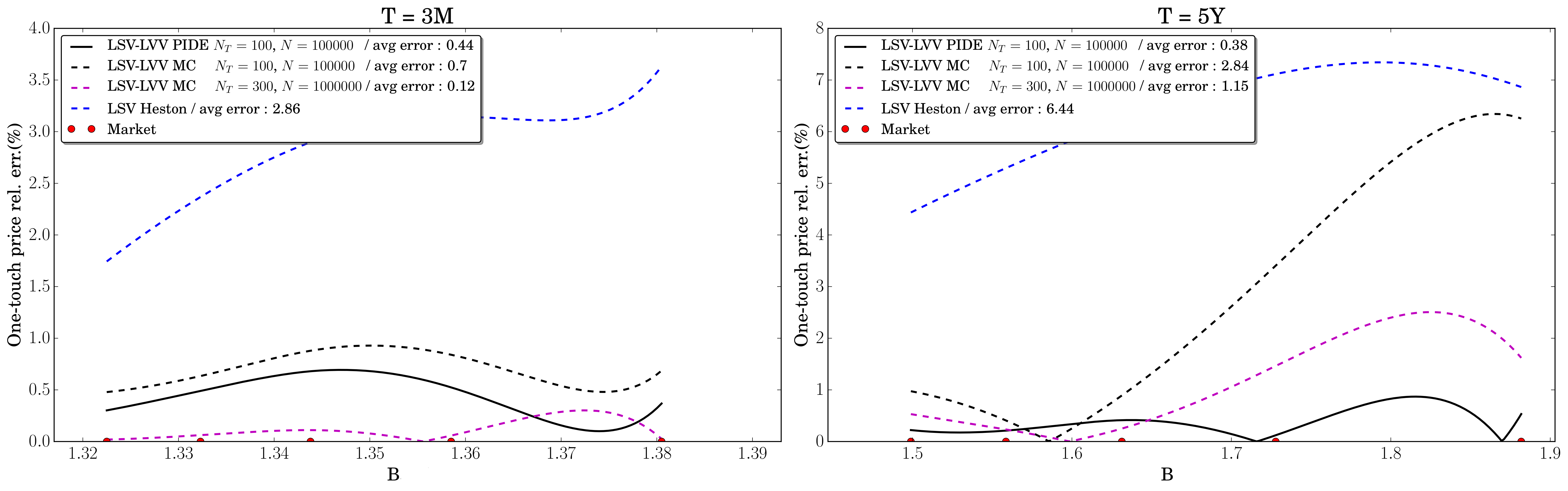
Figure 5.3: Full Monte Carlo vs forward PIDE calibration comparison for a short- and long-term maturity pillar, $N_{T}$ is the number of time steps per year and $N$ the number of particles.

?figurename? 5.4: Local vol-of-vol $\xi\mathopen{}\mathclose{{}\left(S,t}\right)$ function calibrated by forward PIDE 200 strike points, 100 000 particles and 100 time steps per year.

?figurename? 5.5: Local vol-of-vol function $\xi\mathopen{}\mathclose{{}\left(S,t}\right)$ calibrated by full Monte Carlo, 500 000 particles and 100 time steps per year.

6 Calibration results and model comparison

In this section, we present the calibration fit for all models in this paper, benchmarked against some widely used models. The calibration error for vanilla options is given in Table 6.1, and for foreign no-touch options in Table 6.2, for both path-dependent models, i.e. the LMV model (4.1) and LMSV model (4.2), as well as the LSV-LVV model (2.5) and the standard LSV model (2.4) with mixing factor $\beta$. As a benchmark, we also include the pure local volatility model, i.e. (2.4) with $\beta=0$, and the LSV Heston model, i.e. (2.4) with $\beta=1$, calibrated to vanilla options and where the Heston parameters are also calibrated to call options.

The average error in absolute implied volatility for vanillas is $0.005\%$ for the LMV model, $0.009\%$ for the LMSV model and $0.014\%$ for the LSV-LVV model.

T	LMV	LMSV	LSV-LVV	LSV mix.=0.55	LV	LSV Heston
0.26	0.001	0.008	0.017	0.055	0.001	0.001
0.51	0.003	0.007	0.014	0.040	0.001	0.006
1.01	0.006	0.005	0.016	0.027	0.001	0.005
2.01	0.006	0.005	0.016	0.016	0.000	0.003
3.01	0.005	0.007	0.014	0.011	0.000	0.003
4.01	0.006	0.012	0.013	0.009	0.001	0.005
5	0.006	0.016	0.012	0.005	0.001	0.003

?tablename? 6.1: Average absolute error of implied volatilities in % for the vanilla options for all models.

For the no-touch prices, we display the average absolute error in % for each maturity as

$$e=\frac{1}{Q_{B}}\sum_{l=1}^{Q_{B}}\mathopen{}\mathclose{{}\left|\mathrm{FNT}^{\text{Model}}\mathopen{}\mathclose{{}\left(B_{T^{\text{Mat}},l},T^{\text{Mat}}}\right)-\mathrm{FNT}^{\text{Market}}\mathopen{}\mathclose{{}\left(B_{T^{\text{Mat}},l},T^{\text{Mat}}}\right)}\right|$$

in Table 6.2, where $Q_{B}$ is the number of quoted barriers and $B_{T^{\text{Mat}},l}$, $1\leq l\leq Q_{B}$, the set of quoted barriers (e.g., for an average absolute error of $0.1\%$ and for a market no-touch probability of $70\%$, the model will price it at $70\%\pm 0.1\%$ on average). The fit for the two path-dependent models should theoretically be perfect for all vanilla and barrier contracts, and any mismatches consist in numerical errors and penalisation, while the LSV-LVV is by construction calibrated to vanilla options but has only two further free parameters per maturity to fit five no-touch prices.

In Figure 6.1, we plot as a function of $B$, for fixed $T$, the error

$$e\mathopen{}\mathclose{{}\left(B,T}\right)=\mathopen{}\mathclose{{}\left(\mathrm{FNT}^{\text{Model}}\mathopen{}\mathclose{{}\left(B,T}\right)-\mathrm{FNT}^{\text{Market}}\mathopen{}\mathclose{{}\left(B,T}\right)}\right)\,.$$

All the model prices are computed with $1\,000\,000$ Monte Carlo paths and $365$ time steps per year, where Brownian increments are generated with Sobol sequences and Brownian bridge construction [7]. The running maximum is sampled with the Brownian bridge technique as in Chapter 6 of [18]. We note that to reach faster convergence for pricing, Sobol sequences and Brownian bridge construction can be used naturally as each path is simulated independently.

T	LMV	LMSV	LSV-LVV	LSV mix.=0.55	LV	LSV Heston
0.26	0.012	0.060	0.079	0.834	1.198	0.706
0.51	0.008	0.043	0.140	0.675	1.455	1.454
1.01	0.028	0.047	0.120	0.435	1.605	1.894
2.01	0.029	0.055	0.157	0.123	1.590	2.097
3.01	0.024	0.043	0.148	0.124	1.439	2.186
4.01	0.026	0.055	0.122	0.147	1.420	2.062
5	0.019	0.063	0.166	0.187	1.380	1.960

?tablename? 6.2: Average absolute error in % for foreign no-touch quotes for all models; see Fig. 6.1 for error plots. On the left hand-side are models calibrated to no-touches (LMV, LMSV, LSV-LVV); on the right-hand side models not calibrated on no-touches (LSV mix.=0.55, LV, LSV Heston).

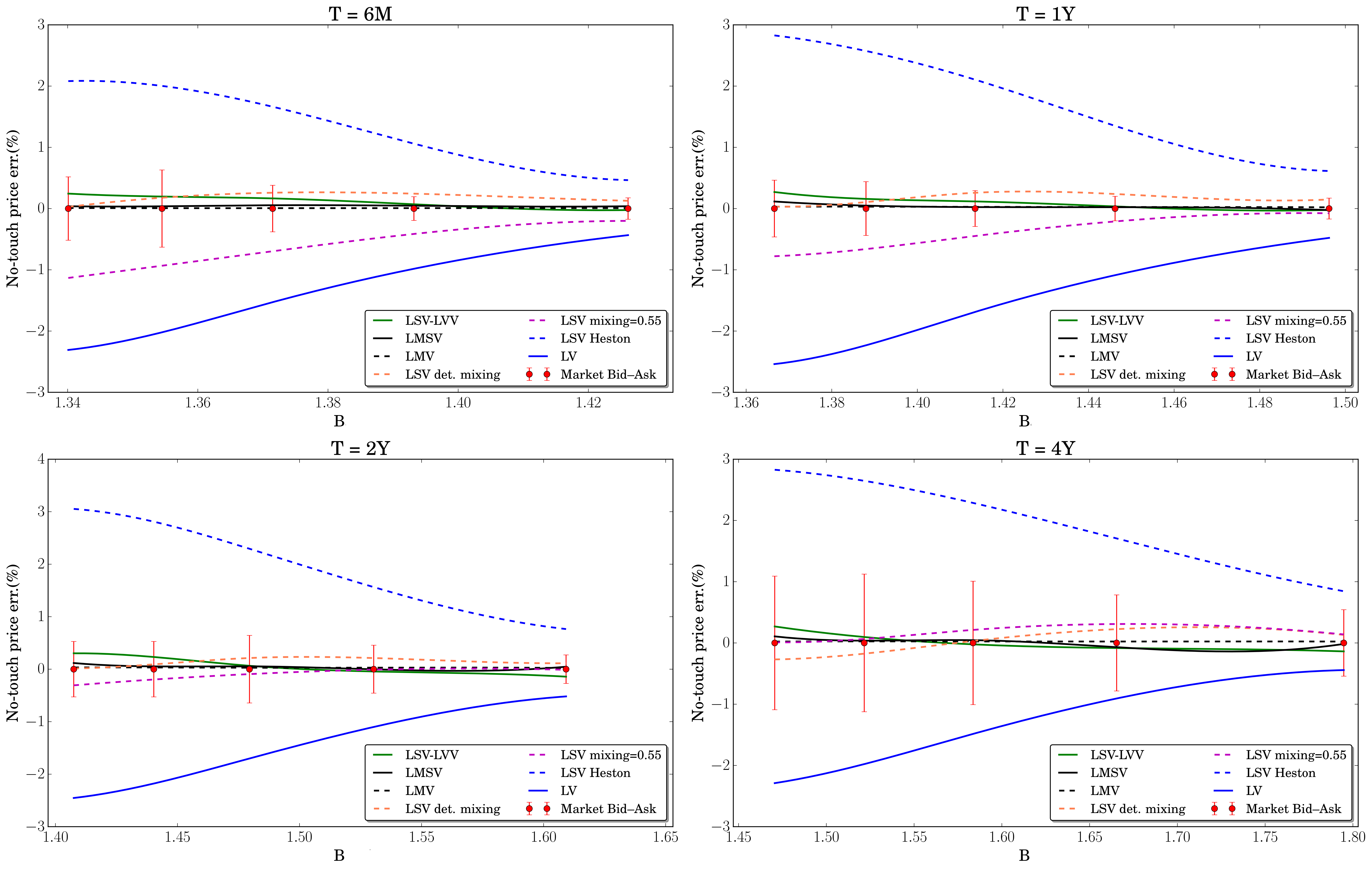
?figurename? 6.1: Calibration fit to foreign no-touch options for all models, as a function of barrier level $B$; see Table 6.2 for tabulated errors.

As Figure 6.1 suggests, if no-touch options are not included in the set of calibration instruments, more classical models like the Heston LSV model can largely mis-price the no-touch probability (in fact, a mis-pricing significantly higher than $3\%$ is common). These results show that the calibration of no-touch options is of paramount importance in order to incorporate the information about the distribution of the running maximum process provided by the market.

The LSV-LVV, LMV and LMSV models, calibrated to both vanilla and foreign no-touch options, perform significantly better for the valuation of no-touch options than the LV or the Heston LSV model calibrated to vanilla options only. The inclusion of a constant mixing factor improves the fit for longer maturities, but still does not allow calibration within the bid–ask spread. This is almost achieved by a time-dependent mixing factor, and fully achieved with a time-dependent vol-of-vol which is also a linear function of the spot FX rate (LSV-LVV model of Section 5).

7 Conclusion

In this work, we demonstrated on the example of three volatility models the calibration to two traded product classes, namely, vanilla and no-touch options.

We introduced a new LSV-LVV model, an extension of the classic Heston-type LSV model with a local vol-of-vol. Due to the small number of degrees-of-freedom, the chosen LSV-LVV parametrisation cannot match no-touch mid-prices perfectly, however, the fit is very satisfactory as the model price lies well within the market spread across all quoted barrier levels and maturities.

We also studied a model based directly on the local maximum mimicking diffusion as the natural extension to the Dupire local volatility framework, namely the LMV model. Then, the addition of a Heston-type stochastic volatility on top of the maximum-dependent volatility leads to a new LMSV model with a potentially more interesting spot-vol dynamics.

Two approaches were proposed for the calibration; one based a two-dimensional particle method to compute the Markovian projection onto the two-dimensional state space $\mathopen{}\mathclose{{}\left(S,M}\right)$, and the other using the numerical solution of a forward PIDE for barrier option prices.

An interesting extension will be to compare the volatility dynamics implied by the three models through the pricing of forward start options. One would then be able to understand to which extent the calibration to touch options, and barriers in general, is compatible with the market smile dynamics.

?appendixname? A Implementation details

A.1 Construction of kernel for particle method

The bandwidth of the one-dimensional Gaussian kernel in (5.3) is given by

$$h_{x}\mathopen{}\mathclose{{}\left(T}\right) = \eta S_{0}{\sigma_{\mathrm{LV}}\mathopen{}\mathclose{{}\left(S_{0},T}\right)}\sqrt{\max\mathopen{}\mathclose{{}\left(T,T_{\min}}\right)}N^{-\frac{1}{6}},$$ (A.1)

where $\sigma_{\mathrm{LV}}\mathopen{}\mathclose{{}\left(S_{0},T}\right)$ is replaced by $\sigma_{\mathrm{LMV}}\mathopen{}\mathclose{{}\left(S_{0},S_{0},T}\right)$ for the LMV model, and

$$\eta=1.5,\,\quad T_{\min}=0.25,\,N_{0}=180.$$

In the two-dimensional case of (4.7), (4.8),

$$h_{y}\mathopen{}\mathclose{{}\left(T}\right) = h_{x}(T)$$

$$\rho_{xy}\mathopen{}\mathclose{{}\left(T}\right) = \mathopen{}\mathclose{{}\left(\rho_{\max}-\hat{\rho}\mathopen{}\mathclose{{}\left(T}\right)}\right)\text{\,exp}\mathopen{}\mathclose{{}\left(-k\frac{N_{T}}{T_{\max}}}\right)+\hat{\rho}\mathopen{}\mathclose{{}\left(T}\right)$$

$$k = \frac{2T_{\max}\ln\mathopen{}\mathclose{{}\left(2}\right)}{N_{0}},$$

where $T_{\max}$ is the last quoted maturity, $\hat{\rho}\mathopen{}\mathclose{{}\left(T}\right)$ the correlation between $S_{T}$ and $M_{T}$ estimated with the sampled particles at time $T$, and $\rho_{\max}=0.98$. To speed up the computation, it is enough to update $\hat{\rho}\mathopen{}\mathclose{{}\left(T}\right)$ once every year or half-year. The use of an appropriate bandwidth was found to have a significant impact on the accuracy of the method. This bandwidth is inspired by a Silverman-type rule (see [37], [22]) for the values of $h_{x}$ and $h_{y}$ and an experimental definition of the correlation part

A heuristic analysis suggests that if the number of time steps is low, the running maximum with the Brownian bridge technique, as described in Chapter 6 of [18], tends to be underestimated in the important area where spot and its running maximum are around the initial values $\mathopen{}\mathclose{{}\left(S_{0},S_{0}}\right)$, since, as seen in Figure 4.6, the local volatility function is an increasing function of the running maximum in this region. Indeed, between two time steps $t$ and $t+\Delta t$, the Brownian bridge technique freezes the value of the volatility function $\sigma_{\text{LMV}}$ from (4.2)for a running maximum $M$ at time $t$ smaller than the value of $M$ along $\mathopen{}\mathclose{{}\left[t,t+\Delta t}\right]$, and therefore, $\sigma_{\text{LMV}}$ is underestimated on average such that $M_{t+\Delta t}$ computed by Brownian bridge is smaller than its exact value.

The intuition behind the specification of the correlation $\rho_{xy}\mathopen{}\mathclose{{}\left(T}\right)$ is as follows: if the number of time steps is low, the running maximum will tend to be underestimated, hence, we give more importance to the particles where the running maximum is higher (which happens when the spot increases); if the number of time steps is large enough, i.e. more than one per day, the running maximum bias is lower and we rely on the sample correlation. It is important to mention that in practice, $\hat{\rho}\mathopen{}\mathclose{{}\left(T}\right)$ is around $80\%\pm 5\%$ and does not change significantly over time. Also, the closer we get to the boundary $S=M$, the higher the correlation, which can easily reach $95\%$. This is due to the fact that for particles where $M$ is large, it is highly probable that $S$ is large as well, therefore, most of the particles will gather around the diagonal boundary. Conversely, if $M$ is around $S_{0}$, most particles are for spots going downwards. This is easily observed from the $\mathopen{}\mathclose{{}\left(S_{t},M_{t}}\right)$ joint density where the mass aggregates around the area $\mathopen{}\mathclose{{}\left(S_{0},S_{0}}\right)$, the line $S=M$ and the line $M=S_{0}$ as displayed in Figure 4.5 where we plot the density computed with a finite element method.

A.2 Particle search on tree

For a given level of spot and running maximum, $K$ and $B$, we only want to compute the kernel function in (4.7) for particles which give a significant contribution to the sum, i.e. particles close enough with respect to the metric implied by $\delta_{N}$. We measure this by $\delta_{N}\mathopen{}\mathclose{{}\left(x,y,T}\right)\leq\epsilon_{0}$ for some $\epsilon_{0}>0$, i.e. all the points contained in the ellipse $\mathcal{E}$ defined by

$$x^{2}+y^{2}-2\rho_{xy}\mathopen{}\mathclose{{}\left(T}\right)xy-H\mathopen{}\mathclose{{}\left(T}\right) = 0\,,$$

with

$$H\mathopen{}\mathclose{{}\left(T}\right)=-2h_{x}^{2}\mathopen{}\mathclose{{}\left(T}\right)\ln\mathopen{}\mathclose{{}\left(\gamma\mathopen{}\mathclose{{}\left(T}\right)\epsilon_{0}}\right)\,.$$

where $\gamma$ is defined in (4.8). The canonical form of ellipse $\mathcal{E}$ expressed in the coordinate system defined by its principal axes is (see [3])

$$\frac{x^{2}}{-D/\mathopen{}\mathclose{{}\left(\lambda_{1}^{2}\lambda_{2}}\right)}+\frac{y^{2}}{-D/\mathopen{}\mathclose{{}\left(\lambda_{1}\lambda_{2}^{2}}\right)}=1\,,$$

with $D=-H\mathopen{}\mathclose{{}\left(T}\right)\mathopen{}\mathclose{{}\left(1-\rho_{xy}^{2}\mathopen{}\mathclose{{}\left(T}\right)}\right)$, $\lambda_{1}=1-\rho_{xy}\mathopen{}\mathclose{{}\left(T}\right)$ and $\lambda_{2}=1+\rho_{xy}\mathopen{}\mathclose{{}\left(T}\right)$, the roots of $\lambda\rightarrow\lambda^{2}-2\lambda+\mathopen{}\mathclose{{}\left(1-\rho_{xy}^{2}\mathopen{}\mathclose{{}\left(T}\right)}\right)$. Since $\rho_{xy}\mathopen{}\mathclose{{}\left(T}\right)\geq 0$ , the semi-major axis length is

$$R\mathopen{}\mathclose{{}\left(T}\right)=\sqrt{-D/\mathopen{}\mathclose{{}\left(\lambda_{1}^{2}\lambda_{2}}\right)}=\sqrt{\frac{H\mathopen{}\mathclose{{}\left(T}\right)}{1-\rho_{xy}\mathopen{}\mathclose{{}\left(T}\right)}}.$$

Working for simplicity with the Euclidean distance, the particles with a significant contribution to the value of $\hat{p}_{N}\mathopen{}\mathclose{{}\left(K,B,T}\right)$ are contained in the ball with center $\mathopen{}\mathclose{{}\left(K,B}\right)$ and radius $R\mathopen{}\mathclose{{}\left(T}\right)$. We use $\epsilon_{0}=\mathopen{}\mathclose{{}\left({\xi\epsilon}}\right)/{10}$ in our tests. A large value of $\epsilon_{0}$ leads to a fast computation of $\hat{p}_{N}$ but also reduces the accuracy of the result.

In order to perform a distance query efficiently, we build a $k$-d tree as described in [5], with a worst case complexity of $\mathcal{O}\mathopen{}\mathclose{{}\left(2N\log N}\right)$ and in which we can perform a binary search with complexity $\mathcal{O}\mathopen{}\mathclose{{}\left(\log N}\right)$ on average, to find all particles with distance less than $\epsilon_{0}$. This provides fast access to the nearest neighbours, and, as a consequence, allows to list the particles contained in the ball of centre $\mathopen{}\mathclose{{}\left(K,B}\right)$ and radius $R\mathopen{}\mathclose{{}\left(T}\right)$.

Remark.

In order to further improve the performance, we could define a distance function

$$d\mathopen{}\mathclose{{}\left(\mathbf{x}_{1},\mathbf{x}_{2}}\right)=\sqrt{\mathopen{}\mathclose{{}\left(s_{1}-s_{2}}\right)^{2}+\mathopen{}\mathclose{{}\left(m_{1}-m_{2}}\right)^{2}-2\rho\mathopen{}\mathclose{{}\left(s_{1}-s_{2}}\right)\mathopen{}\mathclose{{}\left(m_{1}-m_{2}}\right)}\,,$$

where the coordinates of a given particle $i$ are given by $\mathbf{x}_{i}=\mathopen{}\mathclose{{}\left[s_{i},\,m_{i}}\right]^{T}$, with $i\in\{1,2\}$ in this example. Then $d$ can be combined with a metric tree algorithm [41] for an optimal nearest neighbours search, by only keeping particles within a distance $H\mathopen{}\mathclose{{}\left(T}\right)$ to the point $\mathopen{}\mathclose{{}\left(K,B}\right)$ of interest. It is straightforward to check that $d$ is in fact a metric.

A.3 Spline interpolation of the volatility surface

We describe here the spline parameterisation of the volatility surfaces for a given time. Let $N_{T}$ be the number of time steps. For a given time $T_{m}$, the function $\sigma$ is approximated on a rectangle $\mathopen{}\mathclose{{}\left[S_{\min}^{m},\,S_{\max}^{m}}\right]\times\mathopen{}\mathclose{{}\left[S_{0},\,S_{\max}^{m}}\right]$, with $S_{\min}^{m}<S_{0}<S_{\max}^{m}$, by bi-variate quadratic splines in the spot and running maximum directions (and piecewise constant in time), and is extrapolated outside these bounds as detailed in Appendix A.4. There are $N_{T}+1$ volatility “slices” in total such that we denote the $m$-th time slice, i.e., $(x,y)\rightarrow\sigma\mathopen{}\mathclose{{}\left(x,y,T_{m}}\right)$, by $\sigma_{m}$.

The surface construction starts by defining a spot grid where we need more grid points around the forward value and less around $S_{\min}^{m}$ and $S_{\max}^{m}$. We then use a hyperbolic grid (see [11] for more details) refined around the forward value

$$F_{m}=S_{0}e^{\int_{0}^{T_{m}}\mathopen{}\mathclose{{}\left(r^{\rm d}\!\!\!\!\;\;(t)-r^{\rm f}\!\!\!\!\;\;(t)}\right)dt}$$

with

$$S_{\min}^{m}=F_{m}e^{-\frac{6}{2}{\sigma_{F}\mathopen{}\mathclose{{}\left(T_{m}}\right)}\sqrt{T_{m}}},\quad S_{\max}^{m}=F_{m}e^{\frac{6}{2}{\sigma_{F}\mathopen{}\mathclose{{}\left(T_{m}}\right)}\sqrt{T_{m}}}\,,$$

where $\sigma_{F}\mathopen{}\mathclose{{}\left(T_{m}}\right)$ is the at-the-money forward volatility of the market for maturity $T_{m}$. The spot grid is denoted by $\mathopen{}\mathclose{{}\left(S_{m,j}}\right)_{m\leq N_{T},\,j\leq N_{S}}$. The creation of the running maximum grid is done selecting the nodes of the spot grid above the initial spot $S_{0}$, which leads to $N_{B}\mathopen{}\mathclose{{}\left(m}\right)\leq N_{S}$, where $N_{B}$ is now time dependent This particular construction is crucial for accuracy as it ensures that the diagonal where $S=M$ is part of the grid, with the associated maximum grid points $\mathopen{}\mathclose{{}\left(M_{m,k}}\right)_{m\leq N_{T},\,k\leq N_{M}\mathopen{}\mathclose{{}\left(m}\right)}$. Each of the grid values can be seen as a parameter and we denote them by $\mathopen{}\mathclose{{}\left(\sigma_{m,j,k}}\right)_{m\leq N_{T},\,j\leq N_{S},k\leq N_{M}\mathopen{}\mathclose{{}\left(m}\right)}$.

A.4 Smooth volatility extrapolation

Here, we describe how we extrapolate volatility functions smoothly to be asymptotically constant in the spatial coordinates from a rectangle $\mathopen{}\mathclose{{}\left[x_{\min},x_{\max}}\right]\times\mathopen{}\mathclose{{}\left[y_{\min},y_{\max}}\right]$. For $\sigma(\cdot,\cdot,t)$ defined on $\mathopen{}\mathclose{{}\left[x_{\min},x_{\max}}\right]\times\mathopen{}\mathclose{{}\left[y_{\min},y_{\max}}\right]$, we first extend the function to $\mathbb{R}^{2}$ by constant extrapolation,

$$\sigma\mathopen{}\mathclose{{}\left(x,y,t}\right)=\sigma\mathopen{}\mathclose{{}\left(\bar{q}_{0}\mathopen{}\mathclose{{}\left(x}\right),\bar{q}_{1}\mathopen{}\mathclose{{}\left(y}\right),t}\right),\qquad(x,y)\in\mathbb{R}^{2},$$

with

$$\bar{q}_{0}\mathopen{}\mathclose{{}\left(x}\right) = x_{\max}\mathbf{1}_{x\geq x_{\max}}+\mathbf{1}_{x<x_{\max}}\mathopen{}\mathclose{{}\left[x_{\min}\mathbf{1}_{x\leq x_{\min}}+x\mathbf{1}_{x>x_{\min}}}\right]$$

$$\bar{q}_{1}\mathopen{}\mathclose{{}\left(y}\right) = y_{\max}\mathbf{1}_{x\geq y_{\max}}+\mathbf{1}_{y<y_{\max}}\mathopen{}\mathclose{{}\left[y_{\min}\mathbf{1}_{y\leq y_{\min}}+y\mathbf{1}_{y>y_{\min}}}\right].$$

From this, we define a linear extrapolation $\sigma$ as

$$\bar{\sigma}\mathopen{}\mathclose{{}\left(x,y,t}\right) = \sigma\mathopen{}\mathclose{{}\left(\bar{q}_{0}\mathopen{}\mathclose{{}\left(x}\right),\bar{q}_{1}\mathopen{}\mathclose{{}\left(y}\right),t}\right)$$

$$+ \mathbf{1}_{x>x_{\max}}\frac{\partial\sigma\mathopen{}\mathclose{{}\left(x_{\max},\bar{q}_{1}\mathopen{}\mathclose{{}\left(y}\right),t}\right)}{\partial x}\mathopen{}\mathclose{{}\left(x-x_{\max}}\right)+\mathbf{1}_{x<x_{\min}}\frac{\partial\sigma\mathopen{}\mathclose{{}\left(x_{\min},\bar{q}_{1}\mathopen{}\mathclose{{}\left(y}\right),t}\right)}{\partial x}\mathopen{}\mathclose{{}\left(x-x_{\min}}\right)$$

$$+ \mathbf{1}_{y>y_{\max}}\frac{\partial\sigma\mathopen{}\mathclose{{}\left(\bar{q}_{0}\mathopen{}\mathclose{{}\left(x}\right),y_{\max},t}\right)}{\partial y}\mathopen{}\mathclose{{}\left(y-y_{\max}}\right)+\mathbf{1}_{y<y_{\min}}\frac{\partial\sigma\mathopen{}\mathclose{{}\left(\bar{q}_{0}\mathopen{}\mathclose{{}\left(x}\right),y_{\min},t}\right)}{\partial y}\mathopen{}\mathclose{{}\left(y-y_{\min}}\right).$$

We then introduce a smoothed transition of the coordinate $x$ at both $x_{\max}$ and $x_{\min}$,

$$q_{0}\mathopen{}\mathclose{{}\left(x}\right)=x_{\max}w\mathopen{}\mathclose{{}\left(x,x_{\max},\eta_{0}}\right)+\mathopen{}\mathclose{{}\left(1-w\mathopen{}\mathclose{{}\left(x,x_{\max},\eta_{0}}\right)}\right)\mathopen{}\mathclose{{}\left[x_{\min}\mathopen{}\mathclose{{}\left(1-w\mathopen{}\mathclose{{}\left(x,x_{\min},-\eta_{0}}\right)}\right)+xw\mathopen{}\mathclose{{}\left(x,x_{\min},-\eta_{0}}\right)}\right]$$ (A.2)

with

$$\begin{cases}w\mathopen{}\mathclose{{}\left(x,x_{0},\eta_{0}}\right)&=\frac{1}{2}(1+\tanh\mathopen{}\mathclose{{}\left(\frac{2x_{0}}{\epsilon}\frac{\mathopen{}\mathclose{{}\left(x-\bar{x}\mathopen{}\mathclose{{}\left(\eta_{0}}\right)}\right)}{\bar{x}\mathopen{}\mathclose{{}\left(\eta_{0}}\right)}}\right)\\ \bar{x}\mathopen{}\mathclose{{}\left(\eta_{0}}\right)&=\frac{2x_{0}^{2}}{2x_{0}+\epsilon\,\text{arctanh}\mathopen{}\mathclose{{}\left(\eta_{0}(1-\frac{\epsilon}{2})}\right)}\\ \epsilon&=\frac{S_{0}}{10}\,,\end{cases}$$

and similar for $y$ at $y_{\max}$ and $y_{\min}$, which we denote $q_{1}$. The idea of the smoothing is to be able to control the impact of the transition on the inside of the domain $\mathopen{}\mathclose{{}\left(x_{\min},x_{\max}}\right)$ by means of the parameter $\eta_{0}$. If $\eta_{0}=1$, most of the transition happens outside of the domain, which allows to match the values of the original function inside the domain. In contrast, if $\eta_{0}=-1$, most of the transition will happen inside the domain. This behaviour can seem attractive at first, however, it will give rise to issues if the function needs to take a specific shape inside the domain, a local volatility for instance. In both cases, we have $q_{0}\mathopen{}\mathclose{{}\left(x_{\max}}\right)\approx x_{\max}$ and $q_{0}\mathopen{}\mathclose{{}\left(x_{\min}}\right)\approx x_{\min}$. Finally, we reach a trade-off when $\eta=0$. This is the value we pick in our implementation. The new volatility is then

$$\bar{\sigma}\mathopen{}\mathclose{{}\left(q_{0}\mathopen{}\mathclose{{}\left(x}\right),q_{1}\mathopen{}\mathclose{{}\left(y}\right),t}\right)\,.$$

An example is shown in Figure 3.6.

?appendixname? B Algorithms

   $\sigma_{\mathrm{LMV}}\mathopen{}\mathclose{{}\left(x,\cdot,T_{1}}\right)=\sigma_{\text{LV}}\mathopen{}\mathclose{{}\left(x,T_{1}}\right),\forall x$

  for  ( $i=1\,;\,i\leq N_{\text{Mat}}\,;\,i{++}$)  do

     while  $\bar{e}>10^{-10}$ and $\mathopen{}\mathclose{{}\left\|\nabla\bar{e}}\right\|>10^{-8}$  do

         solve forward PIDE (2) on $\mathopen{}\mathclose{{}\left[T_{i-1},T_{i}}\right]$ (with $T_{0}=0$)

         compute model implied vol $\Sigma^{\text{Model}}$ for $T_{i}$ from computed up-and-out call prices $C\mathopen{}\mathclose{{}\left(K,B_{\max},T_{i}}\right)$

         compute model foreign no-touch price $\mathrm{FNT}^{\text{Model}}$ for maturity $T_{i}$ from the computed up-and-out call prices $C\mathopen{}\mathclose{{}\left(0,B,T_{i}}\right)/S_{0}$

         compute the objective function

$$\bar{e}\mathopen{}\mathclose{{}\left(\Lambda_{i}}\right)=e\mathopen{}\mathclose{{}\left(\Lambda_{i}}\right)\mathopen{}\mathclose{{}\left(1+\mathcal{P}\mathopen{}\mathclose{{}\left(\Lambda_{i}}\right)}\right)$$

as in (4.1)

         compute the objective function gradient $\nabla\bar{e}\mathopen{}\mathclose{{}\left(\Lambda_{i}}\right)$ using the forward PIDE solution for $\nabla C\mathopen{}\mathclose{{}\left(\Lambda_{i}}\right)$

         update volatility surface points $\Lambda_{i}$ with the L-BFGS-B algorithm

     end while

      set $\sigma_{\mathrm{LMV}}\mathopen{}\mathclose{{}\left(x,y,T_{i+1}}\right)=\sigma_{\mathrm{LMV}}\mathopen{}\mathclose{{}\left(x,y,T_{i}}\right),\forall\mathopen{}\mathclose{{}\left(x,y}\right)$

  end for

Algorithm 1 Calibration of the local maximum volatility model

Algorithm 2 Calibration of path-dependent $\sigma$ with 2D particle method

1:   $\sigma\mathopen{}\mathclose{{}\left(S,M,T_{0}=0}\right)=\frac{\sigma_{\mathrm{LMV}}\mathopen{}\mathclose{{}\left(S,M,0}\right)}{\sqrt{v_{0}}}$

2:  for each time point ( $m=0\,;\,m\leq N_{T}-1\,;\,m{++}$)  do

3:      generate $\mathopen{}\mathclose{{}\left(Z,Z_{v}}\right)_{i\leq N}$ and $\mathopen{}\mathclose{{}\left(U_{v},U_{\max}}\right)_{i\leq N}$, i.e. $2\times N$ independent draws from $\mathcal{N}\mathopen{}\mathclose{{}\left(0,1}\right)$ and $2\times N$ draws from $\mathcal{U}\mathopen{}\mathclose{{}\left(\mathopen{}\mathclose{{}\left[0,1}\right]}\right)$, respectively

4:      evolve the 2-factor 3-state particle system from $T_{m}$ to $T_{m+1}$ with the $QE-$Scheme ($Z,Z_{v},U_{v}$) where the running maximum is computed by Brownian bridge ($U_{\max}$) and where $\sigma\mathopen{}\mathclose{{}\left(S,M,\mathopen{}\mathclose{{}\left[T_{m},T_{m+1}}\right[}\right)=\sigma\mathopen{}\mathclose{{}\left(S,M,T_{m}}\right)$

5:      build the particles $k$-d tree partitioning on the position values $\mathopen{}\mathclose{{}\left(S^{i}\,,M^{i}}\right)$ as described in Appendix A.1.

6:      set $T=T_{m+1}$

7:     for each maximum level( $k=1\,;\,k\leq N_{M}\,;\,k{++}$)  do

8:        for each spot level ( $j=1\,;\,j\leq N_{S}\,;\,j{++}$)  do

9:            set $K=S_{m+1,j}$; $B=M_{m+1,k}$

10:            select using the $k$-d tree, a set of selected significant particles $I(K,B)$

11:           if  ($K\leq B$)  then

12:               compute and update

$$\hat{p}_{N}=\frac{\frac{1}{\mathopen{}\mathclose{{}\left|I\mathopen{}\mathclose{{}\left(K,B}\right)}\right|}\sum_{i\in I\mathopen{}\mathclose{{}\left(K,B}\right)}V_{T}^{i}\delta_{N}\mathopen{}\mathclose{{}\left(S_{T}^{i}-K,\,M_{T}^{i}-B,T}\right)+2\theta\xi\epsilon}{\frac{1}{\mathopen{}\mathclose{{}\left|I\mathopen{}\mathclose{{}\left(K,B}\right)}\right|}\sum_{i\in I\mathopen{}\mathclose{{}\left(K,B}\right)}\delta_{N}\mathopen{}\mathclose{{}\left(S_{T}^{i}-K,\,M_{T}^{i}-B,T}\right)+\xi\epsilon}$$

13:           end if

14:            compute

$$\sigma_{m+1,j,k}=\frac{\sigma_{\mathrm{LMV}}\mathopen{}\mathclose{{}\left(K,B,T}\right)}{\sqrt{\hat{p}_{N}}}\,$$

15:        end for

16:     end for

17:  end for

Algorithm 3 Calibration of LSV-LVV $\mathopen{}\mathclose{{}\left(\sigma,\xi}\right)$ with 2D particle method, forward PIDE and inner iterations

1:   $\sigma\mathopen{}\mathclose{{}\left(S,0}\right)=\frac{\sigma_{\mathrm{LV}}\mathopen{}\mathclose{{}\left(S,0}\right)}{\sqrt{v_{0}}}$

2:   $\sigma_{\text{LMV}}\mathopen{}\mathclose{{}\left(S,M,0}\right)=\sigma_{\mathrm{LV}}\mathopen{}\mathclose{{}\left(S,0}\right)$

3:   $N_{T}^{\text{down}}=0$

4:   set$\mathopen{}\mathclose{{}\left(a_{1},b_{1}}\right)=\mathopen{}\mathclose{{}\left(-1,\xi_{\mathrm{H}}}\right)$

5:  for each maturity( $n=1\,;\,n\leq N_{T}^{\text{Mat}}\,;\,n{++}$)  do

6:      set $\mathopen{}\mathclose{{}\left(a_{n},b_{n}}\right)=\mathopen{}\mathclose{{}\left(a_{n-1},b_{n-1}}\right)$

7:      find $N_{T}^{\rm up}$ such that $T_{N_{T}^{\rm up}}=T_{n}^{\text{Mat}}$

8:      set the optimisation variable $\text{\it convergence}=\text{false}$

9:     while  convergence is false  do

10:        for  each time point( $m=N_{T}^{\text{down}}\,;\,m<N_{T}^{\rm up}\,;\,m{++}$)  do

11:            generate $\mathopen{}\mathclose{{}\left(Z,Z_{v}}\right)_{i\leq N}$ and $\mathopen{}\mathclose{{}\left(U_{v},U_{\max}}\right)_{i\leq N}$, i.e., $2\times N$ independent draws from $\mathcal{N}\mathopen{}\mathclose{{}\left(0,1}\right)$ and $\mathcal{U}\mathopen{}\mathclose{{}\left(\mathopen{}\mathclose{{}\left[0,1}\right]}\right)$

12:            evolve the 2-factor 3-state particle system of model (2.5) from $T_{m}$ to $T_{m+1}$ with the QE-Scheme, where the maximum is computed by Brownian bridge ($U_{\max}$) and $\sigma\mathopen{}\mathclose{{}\left(S,\mathopen{}\mathclose{{}\left[T_{m},T_{m+1}}\right[}\right)=\sigma\mathopen{}\mathclose{{}\left(S,T_{m}}\right)$

13:            build, as in Appendix A.2, the $k$-d tree of the particles by their positions $\mathopen{}\mathclose{{}\left(S^{i},\,M^{i}}\right)$. This allows to define a set of significant particles $I\mathopen{}\mathclose{{}\left(K,B}\right)$ to use in (B.1).

14:            set $T=T_{m+1}$

15:            for each $K$ on a grid, compute as in [22, 11] for a set of selected significant particles $I\mathopen{}\mathclose{{}\left(K}\right)$

$$\sigma\mathopen{}\mathclose{{}\left(K,T}\right)=\frac{\sigma_{\mathrm{LV}}\mathopen{}\mathclose{{}\left(K,T}\right)\sqrt{\sum_{i\in I\mathopen{}\mathclose{{}\left(K}\right)}\delta_{N}^{S}\mathopen{}\mathclose{{}\left(S_{T}^{i}-K,T}\right)+2\theta\xi\epsilon}}{\sqrt{\sum_{i\in I\mathopen{}\mathclose{{}\left(K}\right)}V_{T}^{i}\delta_{N}^{S}\mathopen{}\mathclose{{}\left(S_{T}^{i}-K,T}\right)+\xi\epsilon}}\,,$$

with $\delta_{N}^{S}$ a one-dimensional kernel function

16:            for each $\mathopen{}\mathclose{{}\left(K,B}\right)$ on a grid, compute as in Section 4.3 for a set of selected significant particles $I\mathopen{}\mathclose{{}\left(K,B}\right)$ as in Section 4.3

$$\sigma_{\text{LMV}}\mathopen{}\mathclose{{}\left(K,B,T}\right)=\frac{\sigma\mathopen{}\mathclose{{}\left(K,T}\right)\sqrt{\frac{1}{\mathopen{}\mathclose{{}\left|I\mathopen{}\mathclose{{}\left(K,B}\right)}\right|}\sum_{i\in I\mathopen{}\mathclose{{}\left(K,B}\right)}V_{T}^{i}\delta_{N}\mathopen{}\mathclose{{}\left(S_{T}^{i}-K,\,M_{T}^{i}-B,T}\right)+2\theta\xi\epsilon}}{\sqrt{\frac{1}{\mathopen{}\mathclose{{}\left|I\mathopen{}\mathclose{{}\left(K,B}\right)}\right|}\sum_{i\in I\mathopen{}\mathclose{{}\left(K,B}\right)}\delta_{N}\mathopen{}\mathclose{{}\left(S_{T}^{i}-K,\,M_{T}^{i}-B,T}\right)+\xi\epsilon}},$$ (B.1)

where $\delta_{N}$ is a two-dimensional kernel function

17:            solve the forward PIDE for barriers (2) by BDF2 implicit step on $\mathopen{}\mathclose{{}\left[T_{m},T_{m+1}}\right]$ with a volatility of $\sigma_{\text{LMV}}\mathopen{}\mathclose{{}\left(K,B,T_{m+1}}\right)$

18:        end for

19:         compute model foreign no-touch price $\mathrm{FNT}^{\text{Model}}$ for maturity $T_{n}^{\text{Mat}}$ from the up-and-out call prices $C\mathopen{}\mathclose{{}\left(0,B,T_{n}^{\text{Mat}}}\right)$ computed with the PIDE

20:         compute the objective function

$$\bar{e}\mathopen{}\mathclose{{}\left(a_{n},b_{n}}\right)=\sum_{l=1}^{Q_{B}}\mathopen{}\mathclose{{}\left|\mathrm{FNT}^{\text{Model}}\mathopen{}\mathclose{{}\left(B_{T_{n}^{\text{Mat}},l},T_{n}^{\text{Mat}},a_{n},b_{n}}\right)-\mathrm{FNT}^{\text{Market}}\mathopen{}\mathclose{{}\left(B_{T_{n}^{\text{Mat}},l},T_{n}^{\text{Mat}}}\right)}\right|$$

21:         update $\mathopen{}\mathclose{{}\left(a_{n},b_{n}}\right)$ guess with the Nelder–Mead algorithm [32]

22:         check difference with the previous iteration and set $\text{\it convergence}={\text{true}}$ if converged

23:     end while

24:  end for

- [1] L. Andersen. Simple and efficient simulation of the Heston stochastic volatility model. The Journal of Computational Finance, 11(3):1–42, 2008.
- [2] E. Ayache, P. Henrotte, S. Nassar, and X. Wang. Can anyone solve the smile problem. Wilmott Journal, January 2004.
- [3] A. B. Ayoub. The central conic sections revisited. Mathematics Magazine, 66(5):322–325, 1993.
- [4] A. Bain and D. Crisan. Fundamentals of Stochastic Filtering. Stochastic Modelling and Applied Probability. Springer New York, 2008.
- [5] R. A. Brown. Building a balanced -d tree in time. Journal of Computer Graphics Techniques, 4(1):50–68, 2015.
- [6] G. Brunick and S. Shreve. Mimicking an Itô process by a solution of a stochastic differential equation. Annals of Applied Probability, 23(4):1584–1628, 2013.
- [7] R. E. Caflisch, W. Morokoff, and A. B. Owen. Valuation of mortgage-backed securities using Brownian bridges to reduce effective dimension. Journal of Computational Finance, 1:27–46, 1997.
- [8] R. Carmona and S. Nadtochiy. Local volatility dynamic models. Finance and Stochastics, 13(1):1–48, 2009.
- [9] P. Carr and J. Crosby. A class of Lévy process models with almost exact calibration to both barrier and vanilla FX options. Quantitative Finance, 10(10):1115–1136, 2010.
- [10] I. J. Clark. Foreign Exchange Option Pricing: A Practitioner’s Guide. John Wiley & Sons, Chichester, UK, 2010.
- [11] A. Cozma, M. Mariapragassam, and C. Reisinger. Calibration of a four-factor hybrid local-stochastic volatility model with a new control variate particle method. preprint, arXiv:1701.06001, 2017.
- [12] S. Crépey. Tikhonov regularization. In R. Cont, editor, Encyclopedia of Quantitative Finance, pages 1807–1812. John Wiley & Sons, Chichester, UK, 2010.
- [13] B. Dupire. A unified theory of volatility. In P. Carr, editor, Derivatives Pricing: The Classic Collection. Risk Books, London, 2004.
- [14] H. Egger and H. W. Engl. Tikhonov regularization applied to the inverse problem of option pricing: convergence analysis and rates. Inverse Problems, 21(3):1027, 2005.
- [15] B. Fornberg. Generation of finite difference formulas on arbitrarily spaced grids. Mathematics of Computation, 51(184):699–706, 1988.
- [16] M. Giles and R. Carter. Convergence analysis of Crank-Nicolson and Rannacher time-marching. Journal of Computational Finance, 9(4):89–112, 2006.
- [17] M. Giles and P. Glasserman. Smoking adjoints: Fast Monte Carlo Greeks. Risk, 19(1):88–92, 2006.
- [18] P. Glasserman. Monte Carlo Methods in Financial Engineering, volume 53 of Stochastic Modelling and Applied Probability. Springer, 2003.
- [19] A. Griewank and A. Walther. Evaluating derivatives: principles and techniques of algorithmic differentiation. SIAM, second edition, 2008.
- [20] F. Guillaume and W. Schoutens. Heston model: The variance swap calibration. Journal of Optimization Theory and Applications, 161(1):76–89, 2014.
- [21] J. Guyon. Path-dependent volatility. Risk Magazine, September, 2014.
- [22] J. Guyon and P. Henry-Labordère. Being particular about calibration. Risk, 25(1):88, 2012.
- [23] J. Guyon and P. Henry-Labordère. Nonlinear Option Pricing. Chapman and Hall/CRC Financial Mathematics. Chapman and Hall/CRC, Boca Raton, USA, 2013.
- [24] I. Gyöngy. Mimicking the one-dimensional marginal distributions of processes having an Itô differential. Probability Theory and Related Fields, 71(4):501–516, 1986.
- [25] E. Hairer, G. Wanner, and S. P. Nï¿œrsett. Solving Ordinary Differential Equations I: Nonstiff Problems. Springer Series in Computational Mathematics 8. Springer-Verlag, Berlin Heidelberg, 2 edition, 1993.
- [26] B. Hambly, M. Mariapragassam, and C. Reisinger. A forward equation for barrier options under the Brunick & Shreve Markovian projection. Quantitative Finance, 16(6):827–838, 2016.
- [27] N. Jackson, E. Süli, and S. Howison. Computation of deterministic volatility surfaces. Journal of Computational Finance, 2:5–32, 1998.
- [28] A. Langnau. A dynamic model for correlation. Risk, 23(4):74–78, 2010.
- [29] F. A. Longstaff and E. S. Schwartz. Valuing american options by simulation: A simple least-squares approach. Review of Financial Studies, pages 113–147, 2001.
- [30] H. P. McKean. A class of Markov processes associated with nonlinear parabolic equations. Proceedings of the National Academy of Sciences of the United States of America, 56:1907–1911, 1966.
- [31] M. Musiela and M. Rutkowski. Martingale methods in financial modelling. Springer Berlin, 2009.
- [32] J. A. Nelder and R. Mead. A simplex method for function minimization. The Computer Journal, 7(4):308, 1965.
- [33] O. Pironneau. Dupire-like identities for complex options. Compte rendu de l’acadï¿œmie des sciences I, 344:127–133, 2007.
- [34] V. Piterbarg. Markovian projection method for volatility calibration. SSRN preprint 906473, 2006.
- [35] A. Reghai. Breaking correlation breaks. Risk, 23(10):92–97, 2010.
- [36] Y. Ren, D. Madan, and M. Qian Qian. Calibrating and pricing with embedded local volatility models. Risk Magazine, September, 2007.
- [37] B. W. Silverman. Density estimation for statistics and data analysis. Biometrical Journal, 30(7):876–877, 1988.
- [38] A.-S. Sznitman. Ecole d’Eté de Probabilités de Saint-Flour XIX, chapter Topics in propagation of chaos, pages 165–251. Springer, 1991.
- [39] L. Tur. Local volatility calibration with fixed-point algorithm. GDF Suez Trading, Informal discussion, 2014.
- [40] D. J. Wales and J. P. K. Doye. Global optimization by basin-hopping and the lowest energy structures of Lennard-Jones clusters containing up to 110 atoms. The Journal of Physical Chemistry A, 101(28):5111–5116, 1997.
- [41] P. N. Yianilos. Data structures and algorithms for nearest neighbor search in general metric spaces. In Proceedings of the Fifth Annual ACM-SIAM Symposium on Discrete Algorithms (SODA), 1993.
- [42] C. Zhu, R. H. Byrd, P. Lu, and J. Nocedal. Algorithm 778: L-BFGS-B: Fortran subroutines for large-scale bound-constrained optimization. ACM Transactions on Mathematical Software, 23(4):550–560, 1997.