A Streaming Analytics Language
for Processing Cyber Data

Abstract

We present a domain-specific language called SAL (the Streaming Analytics Language) for processing data in a semi-streaming model. In particular we examine the use case of processing netflow data in order to identify malicious actors within a network. Because of the large volume of data generated from networks, it is often only feasible to process the data with a single pass, utilizing a streaming ($O(polylog\,n)$ space requirements) or semi-streaming computing model ( $O(n\cdot polylog\,n)$ space requirements). Despite these constraints, we are able to achieve an average of 0.87 for the AUC of the ROC curve for a set of situations dealing with botnet detection. The implementation of an interpreter for SAL, which we call SAM (Streaming Analytics Machine), achieves scaling results that show improved throughput to 61 nodes (976 cores), with an overall rate of 373,000 netflows per second or 32.2 billion per day. SAL provides a succinct way to describe common analyses that allow cyber analysts to find data of interest, and SAM is a scalable interpreter of the language.

1 Introduction

Cyber security is challenging problem due to the large volume of data that is produced, the changing nature of the data, and the ever evolving threat landscape. Cyber analysts need to extract features from a high-throughput stream, create models that will predict malicious behavior or anomalies, evaluate the results, and iterate in a continuous cycle of improvement and adjustment. Our work provides a domain specify language (DSL) for expressing streaming computations on cyber data, enabling cyber analysts to quickly express machine learning pipelines to analyze and classify the data. The main contribution of this paper is to combine within one DSL the ability to succinctly express streaming operators, vertex-centric graph operations, and machine learning pipelines. We call this language the Streaming Analytics Language (SAL). While this work focuses on detecting malicious activity in high-volume cyber data, SAL can be applied to any streaming problem where the elements of the stream are tuples.

We extract features from a stream of cyber data, where the data generation rate only allows a single pass. Streaming [23] and semi-streaming [23, 11] fit the requirements. However, it is currently cumbersome to express streaming operators as no high-level language currently has them as first-class citizens. Also, it is often desirable to extract queries in terms of nodes within the graph of network activity. For example, we may want to gather statistics about the incoming flow sizes of individual IPs. SAL makes this type of vertex-centric computation easy to express. Once we have features, we can define a machine learning pipeline to conduct either supervised or unsupervised machine learning.

Besides the language itself as a contribution, we also present a scalable implementation that translates SAL into C++ code that runs in parallel on a cluster of machines. We call this interpreter the Streaming Analytics Machine, or SAM. We show scaling to 61 nodes on the real-world problem of identifying malicious traffic from botnets. The example pipeline we describe in this paper can process over 373,000 netflows per second, or about 32.2 billion per day. We apply the pipeline to CTU-13 [13], which contains 13 botnet scenarios. Classifying at a per-netflow basis, across this dataset we achieve an average area under the curve (AUC) of the receiver operating characteristic curve (ROC) of 0.87 with the median being 0.90. We envision SAL employed as a filter, so that analysts can concentrate more expensive analysis on a much reduced set.

In Section 2 we present SAL and also walk through a case-study of how SAL can be used to express a pipeline described in another paper [5]. In Section 3 we describe SAM, the implementation we developed to interpret SAL. Section 4 discusses results of detecting malicious activity and Section 5 presents the scaling achieved by the system. Section 6 compares our work to related efforts, and Section 7 concludes.

2 A Language for Streaming and Semi-Streaming Operations

In this section we discuss streaming and semi-streaming algorithms and define how the Streaming Analytics Language expresses those algorithms.

Streaming algorithms is a research area where space and temporal requirements are polylogarithmic (i.e. $O((\log n)^{k})$ for some $k$) [23]. Sometimes those constraints, in particular the temporal complexity, are relaxed [20]. Several algorithms have been published within these constraints: K-medians [4], frequent items [15], mean/frequency counts [21, 8, 34], quantiles [3], rarity [9], variance [4, 34], vector norms [8], similarity [9], and count distinct elements [7, 22].

While some streaming algorithms operate on the entire stream, we focus on the sliding window model, where only recent inputs contribute to feature calculation. We believe the sliding window model is more appropriate for cyber data, where the environment is constantly changing. The sliding window model can also be subcategorized into either a window over a time duration, or by the last $n$ items. Currently SAL only supports expressing windows over the last $n$ items, but many of the underlying algorithms are easily adapted to temporal windows, so support would be easy to add.

Many SAL programs have $O(N\cdot polylog\,n)$ spatial requirements, where $N$ is the number of vertices in the graph (e.g. IPs) and $n$ is the size of the sliding window. Generally each vertex undergoes a set of polylogarithmic operations. This is similar to semi-streaming [23, 11] which has $O(n\cdot polylog\,n)$ spatial requirements for graph algorithms where $n$ is the number of vertices.

SAL is an imperative language. Below is a short example.

Listing 1: SAL code example

⬇

1//Preamble Statements

2WindowSize = 1000;

3

4// Connection Statements

5Netflows = VastStream(”localhost”, 9999);

6

7// Partition Statements

8PARTITION Netflows By SourceIp, DestIp;

9HASH SourceIp WITH IpHashFunction;

10HASH DestIp WITH IpHashFunction;

11

12// Pipeline Statements

13VertsByDest = STREAM Netflows BY DestIp;

14Feature1 = FOREACH VertsByDest GENERATE ave(SrcTotalBytes);

15Filtered = FILTER VertsByDest BY Feature1 > 1000

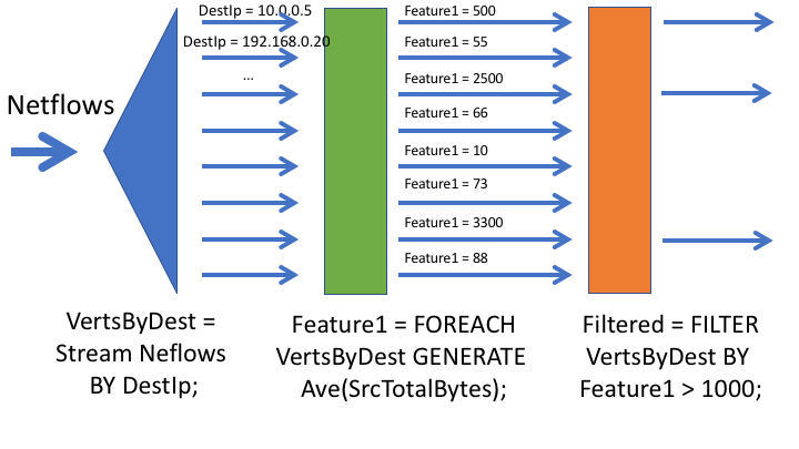
Figure 1: Visual representation of the SAL program in Listing 1.

Each SAL program has four parts: preamble, partition, connection, and pipeline statements. Preamble statements allow for global constants to be defined that are used throughout the program. In the above listing, line 2 defines the default window size, i.e. the number of items in the sliding window.

After the preamble are the connection statements. Line 5 defines a stream of netflows called Netflows. VastStream tells the SAL interpreter to expect netflow data of a particular format (we use the same format for netflows as found in the VAST Challenge 2013: Mini-Challenge 3 dataset [32]). Each participating node in the cluster receive netflows over a socket on port 9999. The VastStream function creates a stream of tuples that represent netflows. For the tuples generated by VastStream, keywords are defined to access the individual fields of the tuple.

There are several different standard netflow formats. SAL currently supports one; however, adding other netflow formats is straightforward. You define a C++ std::tuple with the required fields and a function object that accepts a string and returns an std::tuple. Once a mapping is defined from the desired keyword (e.g. VastStream) to the std::tuple, this new tuple type can be used in SAL connection statements. The mapping is defined via the Scala Parser Combinator [26].

Following the connection statements is the definition of how the tuples are partitioned across the cluster. Line 8 specifies that the netflows should be partitioned separately by SourceIp and DestIp. Each node in the cluster acts as an independent sensor and receives a separate stream of netflows. These independent streams are then re-partitioned across the cluster. In this example, each node is assigned a set of Source IP’s and Destination IP’s using a common hash function. Hash functions can be defined and mapped to SAL constructs, similar to how other tuples can be added to SAL. The process is to define a function object that accepts the tuple type and returns an integer, and then map the function object to a keyword using the Scala Parser Combinator.

The last part of a SAL program is the pipeline statements which describe how the data is to be processed. Line 13 logically separates the single Netflow stream into multiple streams using STREAM $<$StreamName$>$ BY $<$Key1, …$>$. In the above example, netflows are separated into streams by the destination IP address, as can be seen in Figure 1. Only fields that were defined in the partition statement can be used in the BY clause.

Separating out the netflows by a given set of keys allows the collection of features based on those keys. Line 14 of Listing 1 demonstrates creating a feature on the separated streams. For each destination IP address $x$, an average is computed on the total bytes sent to $x$ from any IP in the sliding window. In general, the format for the FOREACH statement is the following:

⬇

<FeatureName> = FOREACH <StreamName> GENERATE <Operator>

The available operators are ave, sum, topk, median, and countdistinct. Each of these operators use a single pass and require polylogarithmic space.

Line 15 gives an example of a FILTER statement. The filter statement allows conditional down-selection of tuples. Filtered is a partitioned stream of netflows, partitioned by destination IP, and then down-selected to only allow netflows through where the average source total bytes is greater than 1000.

Each SAL pipeline has two operating modes: training and testing. In training, the pipeline is run against a finite set of data with labels, and any features created by the pipeline will be appended per input tuple. This feature set along with the labels is used to train a classifier offline. The testing phase then applies the pipeline to a live stream, transforming each tuple into features, and then applies the trained classifier to the features to assign a label.

2.1 Case Study

In this section, we take a look at one approach at creating a classifier for detecting botnets, namely Disclosure [5]. This will help elucidate how SAL can be used to create succinct representations of machine learning pipelines that previously were developed in an ad-hoc fashion. Also, it will demonstrate what cannot be expressed by SAL. Some of the features created by Disclosure require algorithms that do not comply with the desired constraints of streaming and semi-streaming. As such those features cannot be created with SAL. However, our intent with SAL is to down-select the stream of data to something more manageable for more intensive study.

A common architecture for botnets is to have a small set of command and control (C&C) servers that issue commands to a large number of infected machines, that then perform attacks such as distributed denial-of-service, stealing data, spam [28], etc. Disclosure focuses on identifying C&C botnet servers.

The first part of the Disclosure pipeline identifies servers. They define servers as an IP address where the top two ports account for 90% of the flows. This can be expressed in SAL with the TopK operator, as in the following example:

⬇

VertsByDest = STREAM Netflows BY DestIp;

Top2 = FOREACH VertsByDest GENERATE topk(DestPort,10000,1000,2);

Servers = FILTER VertsByDest BY

top2.value(0) + top2.value(1) > 0.9;

As before in Listing 1, we stream the netflows by destination IP. Then with a FOREACH GENERATE statement combined with the topk streaming operator, we calculate an estimate on the top two ports that receive traffic for each destination IP. We then follow that with a filter. The value(n) function returns the frequency of the $n^{th}$ most frequent item (zero-based indexing).

Once the servers have been determined, the authors of Disclosure hypothesized that flow size distributions for C&C servers are distinguishable from benign servers. An example they give is that C&C generally have a limited number of commands, and thus flow sizes are limited to a small set of values. On the other hand, benign servers will generally have a much wider range of values. To detect these difference between C&C servers and benign servers, they create three different types of features based on flow size: statistical features, autocorrelation and unique flow sizes. For the statistical features, they extract the mean and standard deviation for the size of incoming and outgoing flows for each server. This is easy to express in SAL as seen below. For each IP in the set of servers, we use the FOREACH GENERATE statement combined with either the ave operator or var operator.

⬇

FlowsizeSumIn = FOREACH Servers GENERATE ave(SrcTotalBytes);

FlowsizeSumOut = FOREACH Servers GENERATE ave(DestTotalBytes);

FlowsizeVarIn = FOREACH Servers GENERATE var(SrcTotalBytes);

FlowsizeVarOut = FOREACH Servers GENERATE var(DestTotalBytes);

Disclosure also generates features using autocorrelation on the flow sizes. The idea is that C&C servers often have periodic behavior that an autocorrelation calculation would illuminate. For each server, the sequence flow sizes can be thought of as a time series. They divide this signal up into 300 second intervals and calculate the autocorrelation of the time series. Unfortunately, we are not aware of a streaming algorithm for calculating autocorrelation. As such, we currently do not allow autocorrelation to be expressed within SAL; mixing algorithms with vastly different spatial and temporal complexity requirements would negate many of the benefits of the language. However, if space is not an issue, adding autocorrelation would be straightforward.

The final set of features based on flow-sizes involves finding the set of unique flow sizes. The hypothesis here is that botnets have a limited set of messages, and so the number of unique flow sizes will be smaller than a typical benign server. To find an estimate on the number of unique flow sizes, one can use the countdistinct operator:

⬇

UniqueIn = FOREACH Servers GENERATE countdistinct(SrcTotalBytes);

UniqueOut = FOREACH Servers GENERATE countdistinct(DestTotalBytes);

However, Disclosure goes a step further. They create an array with the counts for each unique element and then compute unspecified statistical features on this array. While this is not exactly expressible in SAL, and having an exact answer would break our space constraints, one could use TopK to obtain estimated counts for the most frequent elements.

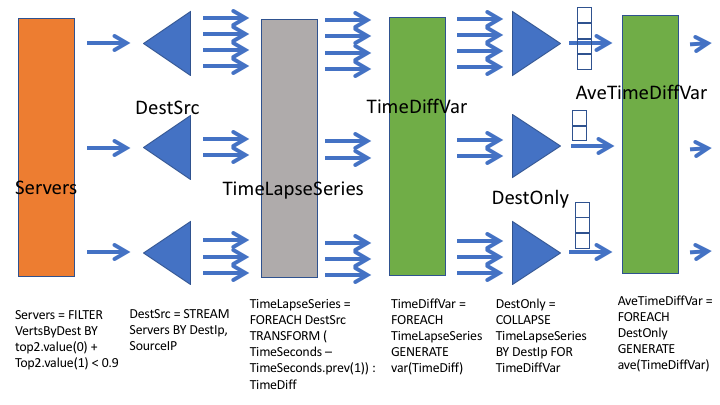
Figure 2: This figure demonstrates the use of the TRANSFORM and COLLAPSE BY statements to define parts of the Disclosure pipeline.

Besides features based on flow size, Disclosure also computes features on client access patterns. The hypothesis is that all the bots accessing a particular C&C server will exhibit very similar behavior, while the behavior of clients accessing benign servers will not be so uniform. Disclosure defines a time series for each server-client pair by calcuating the inter-arrival times between consecutive connections. For example, if we had $n$ netflows that occurred at times $t_{0}$, $t_{1}$, … $t_{n}$, then the series would be $t_{1}-t_{0}$, $t_{2}-t_{1}$, …,$t_{n}-t_{n-1}$. To specify this time series in SAL, one uses the TRANSFORM statement. The TRANSFORM statement allows one to transform from one tuple representation to another.

For this example, we need to transform from the original netflow tuple representation to a tuple that has three values: the SrcIp, DestIp, and the inter-arrival time. In the listing below, we first use the STREAM BY statement to further seprate the stream of netflows into source-destination IP pairs. Then we follow that with the the TRANSFORM statement that calculates the inter-arrival time. Since SourceIp and DestIp are the keys defined by the STREAM BY statement, those values are included by default as the first two values of the newly defined tuple. This part of the pipeline is represented in the left side of Figure 2.

In the example below, we introduce the $prev(i)$ function. The $prev(i)$ function returns the value of the related field $i$ items back in time. $TimeSeconds.prev(1)$ returns the value of $TimeSeconds$ in the tuple that occurred previous to the current tuple, thus giving us the inter-arrival time. The colon followed by TimeDiff gives a label to the tuple value and can be referred to in later SAL statements.

⬇

DestSrc = STREAM Servers BY DestIp, SourceIp;

TimeLapseSeries = FOREACH DestSrc TRANSFORM

(TimeSeconds - TimeSeconds.prev(1)) : TimeDiff

Now that we have the time series expressed in SAL, we can then add the feature extraction methods that Disclosure performs on the inter-arrival times. Disclosure calculates the minimum, maximum, median, and standard deviation. The median and standard deviation can be expressed in SAL below:

⬇

TimeDiffVar = FOREACH TimeLapseSeries GENERATE var(TimeDiff);

TimeDiffMed = FOREACH TimeLapseSeries GENERATE median(TimeDiff);

However, maximum and minimum are not currently supported in SAL. The reason is that max and min require $O(n)$ space where $n$ is the size of the window when computing over a sliding window [8]. When computing over the entire data stream, to compute the max/min one can keep track of one number, but the sliding window adds complexity as the max/min expires. Perhaps some mixture between the two models, over the entire stream and sliding windows, would be sufficient for creating features. Also, as with autocorrelation, if space is not an issue, adding max and min is an easy extension.

For the features derived from the time series to be applicable to classifying servers, we need to combine the features from all the clients. To do so, we no longer use SourceIp as one of the keys to separate the data flow by using the COLLAPSE BY statement. The BY clause contains a list of keys that are kept. Unspecified keys are removed from the key set. Below, DestIp is kept while SourceIp is not specified, meaning that it is no longer a key to separate the data.

⬇

DestOnly = COLLAPSE TimeLapseSeries BY DestIp FOR TimeDiffVar,

TimeDiffMed;

There are different possibilities for the semantics of the COLLAPSE BY statement. The one that we have implemented is the following: Let $k_{+}$ be the tuple elements that are kept by COLLAPSE, and let $k_{-}$ be the tuple elements that are no longer used as a key. For each tuple $t$ that appears in the stream $S$ of data, let $k_{+}(t)$ be the subtuple with only tuple elements from $k_{+}$, and let $k_{-}(t)$ be the subtuple with only tuple elements from $k_{-}$. Also, let $r(t)$ be the subtuple with remaining elements that are neither in $k_{+}(t)$ nor in $k_{-}(t)$. Define $L$ to be the set of unique $k_{+}(t)$ for all $t\in S$, i.e. $L=\bigcup_{t\in S}k_{+}(t)$ For each $l\in L$, we define another set, $M_{l}$: $M_{l}=\bigcup_{t\in S,k_{+}(t)=l}k_{-}(t)$ COLLAPSE BY creates a mapping for each set $M_{l}$, mapping the elements of $M_{l}$ to the most recently seen $r(t)$ associated with each $m\in M_{l}$. These mappings can then be operated on by the FOREACH GENERATE statement.

Once we have collapsed back to DestIp, we can then calculate statistics across the set of clients for each server. The Disclosure paper does not specify which statistics are calculated, but below we give some examples.

⬇

AveTimeDiffVar = FOREACH DestOnly GENERATE ave(TimeDiffVar);

VarTimeDiffVar = FOREACH DestOnly GENERATE var(TimeDiffVar);

That concludes our exploration of how SAL can be used to express concepts from a real pipeline defined in another paper. While there are some operations that are not supported, e.g. the autocorrelation features and max/min, most of the features could be expressed in SAL. We believe SAL provides a succinct way to express streaming machine learning pipelines. In the next sections we discuss how SAL is interpreted with a specific implementation.

3 Implementation

Here we discuss how SAL runs in parallel across a cluster. We translate SAL with the Scala Parser Combinator Library [26]. We express SAL’s grammar and map those elements to C++ code that utilizes a prototype parallel library that we wrote to execute SAL programs called the Streaming Analytics Machine, or SAM. For the Disclosure pipeline, SAL uses 20 lines of code while SAM needs 520 lines. For another pipeline we discuss in Section 4, SAL requires 34 lines while SAM needs 520. Overall, SAL uses 10-25 times fewer lines.

SAM is architected so that each node in the cluster receives tuple data. Right now for the prototype, the only ingest method is a simple socket layer. In maturing SAM, other options such as Kafka [14] is an obvious alternative. We then use ZeroMQ [1] to distribute the tuples across the cluster.

For each tuple that a node receives, it performs a hash for each key specified in the PARTITION statement, and sends the tuple to the node assigned that key. For our experiments we partition on both source IP and dest IP, meaning that for each netflow a node receives over the socket layer, it sends the same netflow twice over ZeroMQ (if the netflow is not kept locally). Many different messaging styles can be expressed by ZeroMQ. We make use of the push/pull paradigm of ZeroMQ. Each node creates $n-1$ push sockets and $n-1$ pull sockets, where $n$ is the size of the cluster.

Conceptually, many of the statements and operators map to either consumers and/or producers, which we implement with C++ classes. The prototype implementation reads netflow data from a socket, so the class ReadSocket reads from the socket and is considered the original source of the stream. A ZeroMQPushPull instance, acting as a consumer, takes the data from the ReadSocket and distributes the netflow data across the cluster using the push sockets. The same ZeroMQPushPull instance uses the pull sockets to collect the netflows destined for it. It then collects those netflows in a queue and once full, calls a parallel feed method. The feed method provides the contents of the queue to all registered consumers in parallel.

Often consumers generate features. Each node creates a thread-safe feature map to collect features that are generated. The function signatures is as follows:

⬇

updateInsert(string key, string featureName, Feature f)

The key is generated by the key fields specified in the STREAM BY statement. The featureName comes from the identifier specified in the FOREACH GENERATE statement. For example, in the below SAL snippet, the key is created by using a string hash function on the concatenation of the source IP and destination IP. The identifier is Feature1 as specified in the FOREACH GENERATE statement. The scheme for ensuring thread-safety in the feature map comes from Goodman et al. [16].

⬇

DestSrc = STREAM Netflows BY SourceIp, DestIp;

Feature1 = FOREACH DestSrc GENERATE ave(SrcTotalBytes);

The Project class provides the functionality of the COLLPASE statement. The Project class creates features similar to the Feature Creator classes, but they cannot be accessed directly through the API. The features are Map features, in other words the sets $M_{l}$ using the terminology from Section 2.1. These Map features are added to the same feature map used for all other generated features. These Map features can then be used by the CollapsedConsumer class, which can be specified to calculate statistics on the map for each kept key in the stream.

4 Classifier Results

To validate the value of SAL in expressing pipelines and in filtering out benign data, we used a simple program where we separate the netflows two ways, by destination IP and by source IP. Then we create features based on the $ave$ and $var$ streaming operators for each of the fields: $SrcTotalBytes$, $DestTotalBytes$, $DurationSeconds$, $SrcPayloadBytes$, $DestPayloadBytes$, $SrcPacketCount$ and $DestPacketCount$. This results in 28 total features.

We apply this pipeline to CTU-13 [13]. CTU-13 has nice characteristics, including: 1) Real botnet attacks: Virtual machines were created and infected. 2) Real background traffic: Traffic from their university router was captured at the same time as the botnet traffic. The botnet traffic was bridged into the university network. 3) A variety of protocols and behaviors: The scenarios cover a range of protocols that were used by the malware such as IRC, P2P, and HTTP. Also some scenarios sent spam, others performed click-fraud, port scans, DDoS attacks, or Fast-Flux. 4) A variety of bots: The 13 scenarios use 7 different bots.

SAL program inherently encodes historical information. As such we can’t treat each netflow independently and thus can’t create random subsets of the data as is usual in a cross-validation approach. We instead split each scenario into two parts. We want to keep the number of malicious netflows about the same in each part (we need enough examples to train on), so we find the point in the scenario timewise where the malicious examples are balanced. Namely we have two sets, $P_{1}$ and $P_{2}$, where $\forall n_{1}\in P_{1},\forall n_{2}\in P_{2},TimeSeconds(n_{1})<TimeSeconds(n_{2})$ and $|Malicious(P_{1})|\approx|Malicious(P_{2})|$, where $TimeSeconds$ returns the time in seconds of the netflow and $Malicious$ returns a subset of the provided set of all the malicious netflows in the provided set. With each scenario split into two parts, we train on the first part and test on the second part. Then we switch: train on the second and test on the first. We make use of a Random Forest Classifier as implemented in scikit-learn [24].

After generating the 28 features, we performed a greedy search over them to down-select to the most important ones. We added features one at a time until no improvement is found in the average AUC over the 13 scenarios. The following eight features provided the best performance across the 13 scenarios. They are listed in the order they were added using the greedy approach above: 1) Average DestPayloadBytes, 2) Variance DestPayloadBytes, 3) Average DestPacketCount, 4) Variance DestPacketCount, 5) Average SrcPayloadBytes, 6) Average SrcPacketCount, 7) Average DestTotalBytes, and 8) Variance SrcTotalBytes.

Using the above eight features, Figure 3 shows the AUC of the ROC for each of the 13 scenarios. In four scenarios, 1, 3, 6, and 11, training on either half was sufficient for the other half, with AUCs between 0.926 and 0.998. Some scenarios, namely 2, 5, 8, 12, and 13, the first half was sufficient to obtain AUCs between 0.922 and 0.992 on the second half, but the reverse was not true. For scenario 10, training on the second half was predictive of the first half, but not the other way. Scenario 9 had AUCs of 0.820 and 0.887, which is decent, but lackluster compared to the other scenarios. The classifier had issues with scenarios 4 and 7. Scenario 7 did not perform well, probably because there were only 63 malicious netflows. We are not sure why the classifier struggled with scenario 4.

5 Scaling

For our scaling experiments, we use Cloudlab [25], a set of clusters distributed across three sites, Utah, Wisconsin, and South Carolina, where researchers can provision a set of nodes to their specifications. We created an image where our code, SAM, was deployed and working, and then replicated that image to a cluster size of our choice. In particular we make use of the Clemson system in South Carolina. The Clemson system has 16 cores per node, 10 Gb/s Ethernet and 256 GB of memory. We were able to allocate a cluster with 64 nodes.

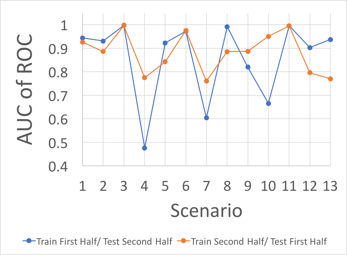
Figure 3: AUC of the ROC

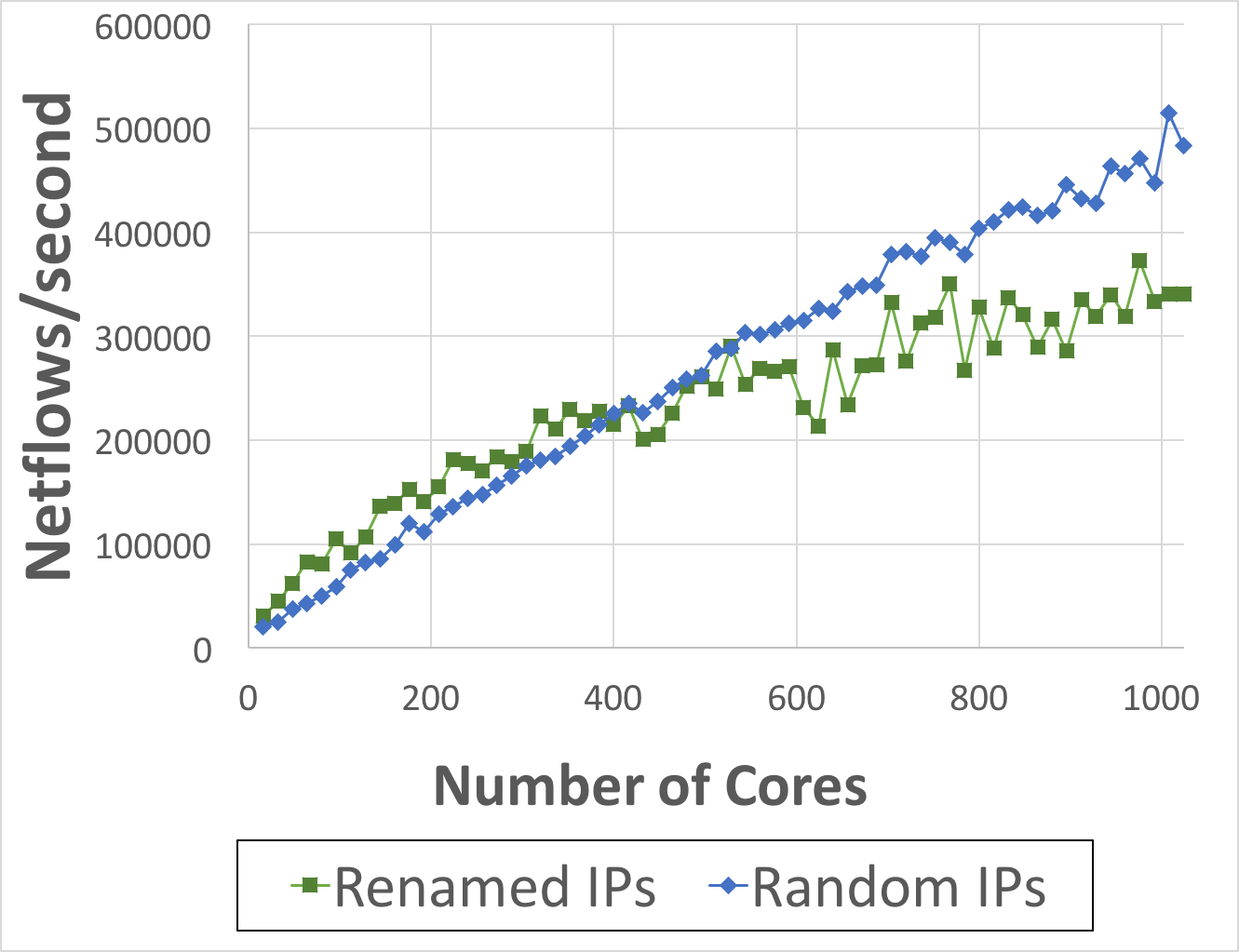
Figure 4: Weak Scaling Results

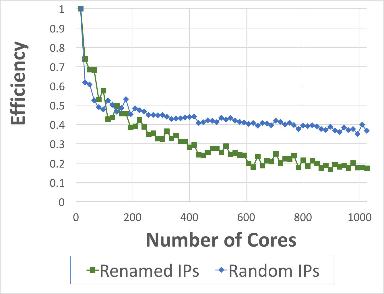
Figure 5: Weak Scaling Efficiency.

Figure 4 shows the weak scaling results. Weak scaling examines the solution time where the problem size scales with the number of nodes, i.e. there is a fixed problem size per node. For our experiments, each node was fed one million netflows. Thus, for $n$ nodes, the total problem size is $n$ million netflows. Each node had available the entire CTU dataset concatenated into one file. Then we randomly selected for each node a contiguous chunk of one million netflows. For each chunk, we renamed the IP addresses to simulate a larger network instead of replaying the same IP addresses, just from different time frames. For comparison we also ran another round with completely random IP addresses, such that an IP address had very little chance of being in multiple netflows. This helped us determine if scaling issues on realistic data were from load balancing problems or some other issue. Each point is the average of three runs.

In Figure 4 we see the renamed IP set of runs peaks out at 61 nodes or 976 cores where we obtain a throughput of 373,000 netflows per second or 32.2 billion per day. For the randomized IP set of runs, the scaling is noticeably steeper, reaching a peak throughput of 515,000 netflows per second (44.5 billion per day) with 63 nodes. Figure 5 takes a look at the weak scaling efficiency. This is defined as $E(n)=T_{1}/T_{n}$, where $T_{i}$ is the time taken by a run with $i$ nodes. Efficiency degrades quicker for the renamed IP set of runs while the randomized IP runs hover close to 0.4. We believe the difference is due to load balance issues. For the randomized IP set of runs, the work is completely balanced between all 64 nodes. The renamed IP runs are more realistic, akin to a power law distribution, where a small set of nodes account for most of the traffic. In this situation, it becomes difficult to partition the work evenly across all the nodes.

As far as we know, we are the first to show scalable distributed network analysis on a cluster of size 64 nodes. The most direct comparison in terms of scaling is Bumgardner and Marek [6]. In this work, they funnel netflows through a 10 node cluster running Storm [30]. They call their approach a hybrid stream/batch system because it uses Storm to stream netflow data into a batch system, Hadoop [17], for analysis. The stream portion is what is most similar to our work. Over the Storm pipeline, they achieve a rate of 234,000 netflows per second, or about 23,400 netflows per second, per node. Our pipeline with ten nodes achieved a rate of 13,900 netflows per second, per node. However, their pipeline is much simpler. They do not partition the netflows by IP and calculate features. The only processing they undergo during streaming is adding subnet information to the netflows, which does not require partitioning across the cluster.

In terms of botnet identification, Botfinder [31] and Disclosure [5] report single node batch performance numbers. Our approach on a single 16-core node achieved a rate of 30,500 netflows per second. For Botfinder, they extract 5 features on a 12 core Intel Core i7 chip, achieving a rate of 46,300 netflows per second. Disclosure generates greater than nine features (the text is ambiguous) on a 16 core Intel Xeon CPU E5630. They specify that they run the feature extraction for one day’s worth of data in 10 hours and 53 minutes, but they do not clearly state if that is on both data sets they chose to evaluate or just one. If it is both, the rate is roughly 40,000 netflows per second.

6 Related Work

There are many frameworks that provide streaming APIs. Prominent among them are Apache Storm [30], Apache Spark [29], Apache Flink [2], and Apache Heron [18]. Each has different advantages and short comings. Many perform checkpointing to allow for replay in case of failure. However, the price of checkpointing may be too significant a cost to justify for our application. Our streaming calculations are by definition approximations, so some lost data may be acceptable. Zhang et al. [33] report success in adapting Storm as the backend of a streaming C-SPARQL engine [12], while Spark has significantly longer latencies. In our own experiments, we found Spark Streaming to have trouble scaling to the node counts we used. We have also experimented with Flink, which has a wealth of implemented streaming concepts that are a natural fit for SAL. So far we’ve found mixed results SAM vs Flink, but that is outside the current scope of this paper will be reported in future work. In any case, our main contribution in this paper is the domain specific language for expressing cyber queries. The underlying implementation can be changed and adapted as technology evolves.

In terms of domain specific languages, there are several graph-related DSL’s that allow for vertex-centric computations, similar to our feature calculations on a per vertex basis. DSL’s like Green-Marl [19] and Ligra [27] provide succint ways to express graph computations, but they are limited to shared-memory infrastructures. Other approaches like Gluon [10] provide a mechanism for converting shared-memory approaches to distributed settings. Regardless of whether these DLS approaches are computationally distributable, a fundamental difference between this set of work and our own is the streaming aspect of our aproach and domain. The algorithmic solutions, partitioning, operation scheduling, and data processing of these graph DSL’s rely upon the assumption of static data. Also, these approaches do not have a way of expressing machine learning pipelines.

7 Conclusions

We have presented a new domain specific language, the Streaming Analytics Language, or SAL, that is designed to easily express analytical pipelines on streaming data. We specifically examined the case of cyber data and showed how it can extract features from netflow data which can then be used to train a classifier using labeled data. Using the CTU-13 dataset as an example, we were able to train classifiers on streaming features that on average obtained an AUC of 0.87. In an operational setting, this could be used to greatly reduce the amount of traffic needing to be analyzed. SAL can be used as a first pass over the data using space and temporally-efficient streaming algorithms. After down-selecting, more expensive algorithms can be applied to the remaining data.

In addition to SAL, we also presented the results of our scalable interpreter of SAL, which we call the Streaming Analytics Machine, or SAM. On real data, we are able to scale to 61 nodes and 976 cores, obtaining a throughput of 373,000 netflows per second or 32.2 billion per day. On completely load-balanced data, we obtain greater efficiency out to 64 nodes than the real data, indicating that SAM could be improved with a more intelligent partitioning strategy. In the end, we have an easy to use domain specific language and a scalable implementation to back it that has good accuracy on the target problem.

References

- [1] Akgul, F.: ZeroMQ. Packt Publishing (2013)
- [2] Apache: Apache flink. flink.apache.org (2018), [Online; accessed June-2018]
- [3] Arasu, A., Manku, G.S.: Approximate counts and quantiles over sliding windows. In: Proceedings of the Twenty-third ACM SIGMOD-SIGACT-SIGART Symposium on Principles of Database Systems. pp. 286–296. PODS ’04, ACM, New York, NY, USA (2004). https://doi.org/10.1145/1055558.1055598, http://doi.acm.org/10.1145/1055558.1055598
- [4] Babcock, B., Datar, M., Motwani, R., O’Callaghan, L.: Maintaining variance and k-medians over data stream windows. In: Proceedings of the Twenty-second ACM SIGMOD-SIGACT-SIGART Symposium on Principles of Database Systems. pp. 234–243. PODS ’03, ACM, New York, NY, USA (2003). https://doi.org/10.1145/773153.773176, http://doi.acm.org/10.1145/773153.773176
- [5] Bilge, L., Balzarotti, D., Robertson, W., Kirda, E., Kruegel, C.: Disclosure: Detecting botnet command and control servers through large-scale netflow analysis. In: Proceedings of the 28th Annual Computer Security Applications Conference. pp. 129–138. ACSAC ’12, ACM, New York, NY, USA (2012). https://doi.org/10.1145/2420950.2420969, http://doi.acm.org/10.1145/2420950.2420969
- [6] Bumgardner, V.K., Marek, V.W.: Scalable hybrid stream and hadoop network analysis system. In: Proceedings of the 5th ACM/SPEC International Conference on Performance Engineering. pp. 219–224. ICPE ’14, ACM, New York, NY, USA (2014). https://doi.org/10.1145/2568088.2568103, http://doi.acm.org/10.1145/2568088.2568103
- [7] Clifford, P., Cosma, I.A.: A statistical analysis of probabilistic counting algorithms. ArXiv e-prints (Jan 2008)
- [8] Datar, M., Gionis, A., Indyk, P., Motwani, R.: Maintaining stream statistics over sliding windows: (extended abstract). In: Proceedings of the Thirteenth Annual ACM-SIAM Symposium on Discrete Algorithms. pp. 635–644. SODA ’02, Society for Industrial and Applied Mathematics, Philadelphia, PA, USA (2002), http://dl.acm.org/citation.cfm?id=545381.545466
- [9] Datar, M., Muthukrishnan, S.: Estimating Rarity and Similarity over Data Stream Windows, pp. 323–335. Springer Berlin Heidelberg, Berlin, Heidelberg (2002)
- [10] Dathathri, R., Gill, G., Hoang, L., Dang, H.V., Brooks, A., Dryden, N., Snir, M., Pingali, K.: Gluon: A communication-optimizing substrate for distributed heterogeneous graph analytics. In: Proceedings of the 39th ACM SIGPLAN Conference on Programming Language Design and Implementation. pp. 752–768. PLDI 2018, ACM, New York, NY, USA (2018). https://doi.org/10.1145/3192366.3192404, http://doi.acm.org/10.1145/3192366.3192404
- [11] Feigenbaum, J., Kannan, S., McGregor, A., Suri, S., Zhang, J.: On graph problems in a semi-streaming model. Theor. Comput. Sci. 348(2), 207–216 (Dec 2005). https://doi.org/10.1016/j.tcs.2005.09.013, http://dx.doi.org/10.1016/j.tcs.2005.09.013
- [12] Francesco Barbieri, D., Braga, D., Ceri, S., Della Valle, E., Grossniklaus, M.: C-sparql: A continuous query language for rdf data streams. International Journal of Semantic Computing 4, 487 (03 2010)
- [13] García, S., Grill, M., Stiborek, J., Zunino, A.: An empirical comparison of botnet detection methods. Computers & Security 45(Supplement C), 100 – 123 (2014). https://doi.org/https://doi.org/10.1016/j.cose.2014.05.011, http://www.sciencedirect.com/science/article/pii/S0167404814000923
- [14] Garg, N.: Apache Kafka. Packt Publishing (2013)
- [15] Golab, L., DeHaan, D., Demaine, E.D., Lopez-Ortiz, A., Munro, J.I.: Identifying frequent items in sliding windows over on-line packet streams. In: Proceedings of the 3rd ACM SIGCOMM Conference on Internet Measurement. pp. 173–178. IMC ’03, ACM, New York, NY, USA (2003). https://doi.org/10.1145/948205.948227, http://doi.acm.org/10.1145/948205.948227
- [16] Goodman, E., Lemaster, M.N., Jimenez, E.: Scalable hashing for shared memory supercomputers. In: Proceedings of 2011 International Conference for High Performance Computing, Networking, Storage and Analysis. pp. 41:1–41:11. SC ’11, ACM, New York, NY, USA (2011). https://doi.org/10.1145/2063384.2063439, http://doi.acm.org/10.1145/2063384.2063439
- [17] Hadoop. hadoop.apache.org (2019)
- [18] Heron. https://github.com/apache/incubator-heron (2019)
- [19] Hong, S., Chafi, H., Sedlar, E., Olukotun, K.: Green-marl: A dsl for easy and efficient graph analysis. In: Proceedings of the Seventeenth International Conference on Architectural Support for Programming Languages and Operating Systems. pp. 349–362. ASPLOS XVII, ACM, New York, NY, USA (2012). https://doi.org/10.1145/2150976.2151013, http://doi.acm.org/10.1145/2150976.2151013
- [20] M. Henzinger, P.R., Rajagopalan, S.: Computing on data stream (May 1998)
- [21] Manku, G.S., Motwani, R.: Approximate frequency counts over data streams. In: Proceedings of the 28th International Conference on Very Large Data Bases. pp. 346–357. VLDB ’02, VLDB Endowment (2002), http://dl.acm.org/citation.cfm?id=1287369.1287400
- [22] Metwally, A., Agrawal, D., Abbadi, A.E.: Why go logarithmic if we can go linear?: Towards effective distinct counting of search traffic. In: Proceedings of the 11th International Conference on Extending Database Technology: Advances in Database Technology. pp. 618–629. EDBT ’08, ACM, New York, NY, USA (2008). https://doi.org/10.1145/1353343.1353418, http://doi.acm.org/10.1145/1353343.1353418
- [23] Muthukrishnan, S.: Data streams: Algorithms and applications. Found. Trends Theor. Comput. Sci. 1(2), 117–236 (Aug 2005). https://doi.org/10.1561/0400000002, http://dx.doi.org/10.1561/0400000002
- [24] Pedregosa, F., Varoquaux, G., Gramfort, A., Michel, V., Thirion, B., Grisel, O., Blondel, M., Prettenhofer, P., Weiss, R., Dubourg, V., Vanderplas, J., Passos, A., Cournapeau, D., Brucher, M., Perrot, M., Duchesnay, E.: Scikit-learn: Machine learning in Python. Journal of Machine Learning Research 12, 2825–2830 (2011)
- [25] Ricci, R., Eide, E., The CloudLab Team: Introducing CloudLab: Scientific infrastructure for advancing cloud architectures and applications. USENIX ;login: 39(6) (Dec 2014), https://www.usenix.org/publications/login/dec14/ricci
- [26] Scala parser combinator. https://github.com/scala/scala-parser-combinators (2017), [Online; accessed October-2017]
- [27] Shun, J., Blelloch, G.E.: Ligra: A lightweight graph processing framework for shared memory. SIGPLAN Not. 48(8), 135–146 (Feb 2013). https://doi.org/10.1145/2517327.2442530, http://doi.acm.org/10.1145/2517327.2442530
- [28] Silva, S.S., Silva, R.M., Pinto, R.C., Salles, R.M.: Botnets: A survey. Computer Networks 57(2), 378 – 403 (2013). https://doi.org/https://doi.org/10.1016/j.comnet.2012.07.021, http://www.sciencedirect.com/science/article/pii/S1389128612003568, botnet Activity: Analysis, Detection and Shutdown
- [29] Spark. spark.apache.org (2019), spark.apache.org
- [30] Storm. storm.apache.org (2019), storm.apache.org
- [31] Tegeler, F., Fu, X., Vigna, G., Kruegel, C.: Botfinder: Finding bots in network traffic without deep packet inspection. In: Proceedings of the 8th International Conference on Emerging Networking Experiments and Technologies. pp. 349–360. CoNEXT ’12, ACM, New York, NY, USA (2012). https://doi.org/10.1145/2413176.2413217, http://doi.acm.org/10.1145/2413176.2413217
- [32] VAST: Vast challenge 2013: Mini-challenge 3. http://vacommunity.org/VAST+Challenge+2013[Online; accessed October-2017]
- [33] Zhang, Y., Chen, R., Chen, H.: Sub-millisecond stateful stream querying over fast-evolving linked data. In: Proceedings of the 26th Symposium on Operating Systems Principles. pp. 614–630. SOSP ’17, ACM, New York, NY, USA (2017). https://doi.org/10.1145/3132747.3132777, http://doi.acm.org/10.1145/3132747.3132777
- [34] Zhu, Y., Shasha, D.: Statstream: Statistical monitoring of thousands of data streams in real time. In: Proceedings of the 28th International Conference on Very Large Data Bases. pp. 358–369. VLDB ’02, VLDB Endowment (2002), http://dl.acm.org/citation.cfm?id=1287369.1287401