Enhanced Convolutional Neural Tangent Kernels††thanks: The first three authors contribute equally.
Abstract
Recent research shows that for training with loss, convolutional neural networks (CNNs) whose width (number of channels in convolutional layers) goes to infinity correspond to regression with respect to the CNN Gaussian Process kernel (CNN-GP) if only the last layer is trained, and correspond to regression with respect to the Convolutional Neural Tangent Kernel (CNTK) if all layers are trained. An exact algorithm to compute CNTK (Arora et al., 2019) yielded the finding that classification accuracy of CNTK on CIFAR-10 is within - of that of the corresponding CNN architecture (best figure being around %) which is interesting performance for a fixed kernel.
Here we show how to significantly enhance the performance of these kernels using two ideas. (1) Modifying the kernel using a new operation called Local Average Pooling (LAP) which preserves efficient computability of the kernel and inherits the spirit of standard data augmentation using pixel shifts. Earlier papers were unable to incorporate naive data augmentation because of the quadratic training cost of kernel regression. This idea is inspired by Global Average Pooling (GAP), which we show for CNN-GP and CNTK is equivalent to full translation data augmentation. (2) Representing the input image using a pre-processing technique proposed by Coates et al. (2011), which uses a single convolutional layer composed of random image patches.
On CIFAR-10, the resulting kernel, CNN-GP with LAP and horizontal flip data augmentation, achieves accuracy, matching the performance of AlexNet (Krizhevsky et al., 2012). Note that this is the best such result we know of for a classifier that is not a trained neural network. Similar improvements are obtained for Fashion-MNIST.
1 Introduction
Recent research shows that for training with loss, convolutional neural networks (CNNs) whose width (number of channels in convolutional layers) goes to infinity, correspond to regression with respect to the CNN Gaussian Process kernel (CNN-GP) if only the last layer is trained, and correspond to regression with respect to the Convolutional Neural Tangent Kernel (CNTK) if all layers are trained (Jacot et al., 2018). An exact algorithm was given (Arora et al., 2019) to compute CNTK for CNN architectures, as well as those that include a Global Average Pooling (GAP) layer (defined below). This is a fixed kernel that inherits some benefits of CNNs, including exploitation of locality via convolution, as well as multiple layers of processing. For CIFAR-10, incorporating GAP into the kernel improves classification accuracy by up to compared to pure convolutional CNTK.
While this performance is encouraging for a fixed kernel, the best accuracy is still under , which is disappointing even compared to AlexNet. One hope for improving the accuracy further is to somehow capture modern innovations such as batch normalization, data augmentation, residual layers, etc. in CNTK. The current paper shows how to incorporate simple data augmentation. Specifically, the idea of creating new training images from existing images using pixel translation and flips, while assuming that these operations should not change the label. Since deep learning uses stochastic gradient descent (SGD), it is trivial to do such data augmentation on the fly. However, it’s unclear how to efficiently incorporate data augmentation in kernel regression, since training time is quadratic in the number of training images.
Thus somehow data augmentation has to be incorporated into the computation of the kernel itself. The main observation here is that the above-mentioned algorithm for computing CNTK involves a dynamic programming whose recursion depth is equal to the depth of the corresponding finite CNN. It is possible to impose symmetry constraints at any desired layer during this computation. In this viewpoint, it can be shown that prediction using CNTK/CNN-GP with GAP is equivalent to prediction using CNTK/CNN-GP without GAP but with full translation data augmentation with wrap-around at the boundary. The translation invariance property implicitly assumed in data augmentation is exactly equivalent to an imposed symmetry constraint in the computation of the CNTK which in turn is derived from the pooling layer in the CNN. See Section 4 for more details.
Thus GAP corresponds to full translation data augmentation scheme, but in practice such data augmentation creates unrealistic images (cf. Figure 1) and training on them can harm performance. However, the idea of incorporating symmetry in the dynamic programming leads to a variant we call Local Average Pooling (LAP). This implicitly is like data augmentation where image labels are assumed to be invariant to small translation, say by a few pixels. This operation also suggests a new pooling layer for CNNs which we call BBlur and also find it beneficial for CNNs in experiments.
Experimentally, we find LAP significantly enhances the performance as discussed below.
-
•
In extensive experiments on CIFAR-10 and Fashion-MNIST, we find that LAP consistently improves performance of CNN-GP and CNTK. In particular, we find CNN-GP with LAP achieves on CIFAR-10 dataset, outperforming the best previous kernel predictor by .
-
•
When using the technique proposed by Coates et al. (2011), which uses randomly sampled patches from training data as filters to do pre-processing,111See Section 6.2 for the precise procedure. CNN-GP with LAP and horizontal flip data augmentation achieves accuracy on CIFAR-10, matching the performance of AlexNet (Krizhevsky et al., 2012) and is the strongest classifier that is not a trained neural network.222 https://benchmarks.ai/cifar-10
-
•
We also derive a layer for CNN that corresponds to LAP and observe that it improves the performance on certain architectures.
2 Related Work
Data augmentation has long been known to improve the performance of neural networks and kernel methods (Sietsma and Dow, 1991; Schölkopf et al., 1996). Theoretical study of data augmentation dates back to Chapelle et al. (2001). Recently, Dao et al. (2018) proposed a theoretical framework for understanding data augmentation and showed data augmentation with a kernel classifier can have feature averaging and variance regularization effects. More recently, Chen et al. (2019) quantitatively shows in certain settings, data augmentation provably improves the classifier performance. For more comprehensive discussion on data augmentation and its properties, we refer readers to Dao et al. (2018); Chen et al. (2019) and references therein.
CNN-GP and CNTK correspond to infinitely wide CNN with different training strategies (only training the top layer or training all layers jointly). The correspondence between infinite neural networks and kernel machines was first noted by Neal (1996). More recently, this was extended to deep and convolutional neural networks (Lee et al., 2018; Matthews et al., 2018; Novak et al., 2019; Garriga-Alonso et al., 2019). These kernels correspond to neural networks where only the last layer is trained. A recent line of work studied overparameterized neural networks where all layers are trained (Allen-Zhu et al., 2018; Du et al., 2019b, 2018; Li and Liang, 2018; Zou et al., 2018). Their proofs imply the gradient kernel is close to a fixed kernel which only depends the training data and the neural network architecture. These kernels thus correspond to neural networks where are all layers are trained. Jacot et al. (2018) named this kernel neural tangent kernel (NTK). Arora et al. (2019) formally proved polynomially wide neural net predictor trained by gradient descent is equivalent to NTK predictor. Recently, NTKs induced by various neural network architectures are derived and shown to achieve strong empirical performance (Arora et al., 2019; Yang, 2019; Du et al., 2019a).
Global Average Pooling (GAP) is first proposed in Lin et al. (2013) and is common in modern CNN design (Springenberg et al., 2014; He et al., 2016; Huang et al., 2017). However, current theoretical understanding on GAP is still rather limited. It has been conjectured in Lin et al. (2013) that GAP reduces the number of parameters in the last fully-connected layer and thus avoids overfitting, and GAP is more robust to spatial translations of the input since it sums out the spatial information. In this work, we study GAP from the CNN-GP and CNTK perspective, and draw an interesting connection between GAP and data augmentation.
3 Preliminaries
3.1 Notation
We use bold-faced letters for vectors, matrices and tensors. For a vector , we use to denote its -th entry. For a matrix , we use to denote its -th entry. For an order tensor , we use to denote its -th entry. For an order tensor, wet use to denote . For an order tensor and an integer , we use to denote the order tensor formed by fixing the coordinate of the last dimension to be .
3.2 CNN, CNN-GP and CNTK
In this section we give formal definitions of CNN, CNN-GP and CNTK that we study in this paper. Throughout the paper, we let be the width and be the height of the image. We use to denote the filter size. In practice, , , or .
Padding Schemes.
In the definition of CNN, CNTK and CNN-GP, we may use different padding schemes. Let be an image. For a given index pair with , , or , different padding schemes define different value for . For circular padding, we define to be . For zero padding, we simply define to be . Note the difference between circular padding and zero padding occurs only on the boundary of images. We will prove our theoretical results for the circular padding scheme to avoid boundary effects.
CNN.
Now we describe CNN with and without GAP. For any input image , after intermediate layers, we obtain where is the number of channels of the last layer. See Section A for the definition of . For the output, there are two choices: with and without GAP.
-
•
Without GAP: the final output is defined as
where , and is the weight of the last fully-connected layer.
-
•
With GAP: the final output is defined as
where is the weight of the last fully-connected layer.
CNN-GP and CNTK.
Now we describe CNN-GP and CNTK. Let be two input images. We denote the -th layer’s CNN-GP kernel as and the -th layer’s CNTK kernel as . See Section A for the precise definitions of and . For the output kernel value, again, there are two choices, without GAP (equivalent to using a fully-connected layer) or with GAP.
-
•
Without GAP: the output of CNN-GP is
and the output of CNTK is
-
•
With GAP: the output of CNN-GP is
and the output of CNTK is
Kernel Prediction.
Lastly, we recall the formula for kernel regression. For simplicity, throughout the paper, we will assume all kernels are invertible. Given a kernel and a dataset with data , define to be . The prediction for an unseen data is where
3.3 Data Augmentation Schemes
In this paper we consider two types of data augmentation schemes: translation and horizontal flip.
Translation.
Given , we define the translation operator as follow. For an image ,
for . Here the precise definition of depends on the padding scheme. Given a dataset , the full translation data augmentation scheme creates a new dataset and training is performed on .
Horizontal Flip.
For an image , the flip operator is defined to be
for . Given a dataset , the horizontal flip data augmentation scheme creates a new dataset of the form and training is performed on .
4 Equivalence Between Augmented Kernel and Data Augmentation
In this section, we demonstrate the equivalence between data augmentation and augmented kernels. To formally discuss the equivalence, we use group theory to describe translation and horizontal flip operators. We provide the definition of group in Section B for completeness.
It is easy to verify that , , are groups, where is the identity map. From now on, given a dataset with data and a group , the augmented dataset is defined to be . The prediction for an unseen data on the augmented dataset is where
To proceed, we define the concept of augmented kernel. Let be a finite group. Define the augmented kernel as
where are two inputs images and is drawn from uniformly at random. A key observation is that for CNTK and CNN-GP, when circular padding and GAP is adopted, the corresponding kernel is the augmented kernel of the group . Formally, we have
and
which can be seen by checking the formula of these kernels and using definition of circular padding. Similarly, the following equivariance property holds for and , under all groups mentioned above, including and .
Definition 4.1.
A kernel is equivariant under a group if and only if for any , .
The following theorem formally states the equivalence between using an augmented kernel on the dataset and using the kernel on the augmented dataset.
Theorem 4.1.
Given a group and a kernel such that is equivariant under , then the prediction of augmented kernel with dataset is equal to that of kernel and augmented dataset . Namely, for any , where .
Corollary 4.1.
For , for any given dataset , the prediction of (or ) with dataset is equal to the prediction of (or ) with augmented dataset .
Corollary 4.2.
For , for any given dataset , the prediction of (or ) with dataset is equal to the prediction of (or ) with augmented dataset .
Now we discuss implications of Theorem 4.1 and its corollaries. Naively applying data augmentation, with full translation on CNTK or CNN-GP for example, one needs to create a much larger kernel matrix since there are translation operators, which is often computationally infeasible. Instead, one can directly use the augmented kernel ( or for the case of full translation on CNTK or CNN-GP) for prediction, for which one only needs to create a kernel matrix that is as large as the original one. For horizontal flip, although the augmentation kernel can not be conveniently computed as full translation, Corollary 4.2 still provides a more efficient method for computing kernel values and solving kernel regression, since the augmented dataset is twice as large as the original dataset, while the kernel matrix of the augmented kernel is as large as the original one.
5 Local Average Pooling
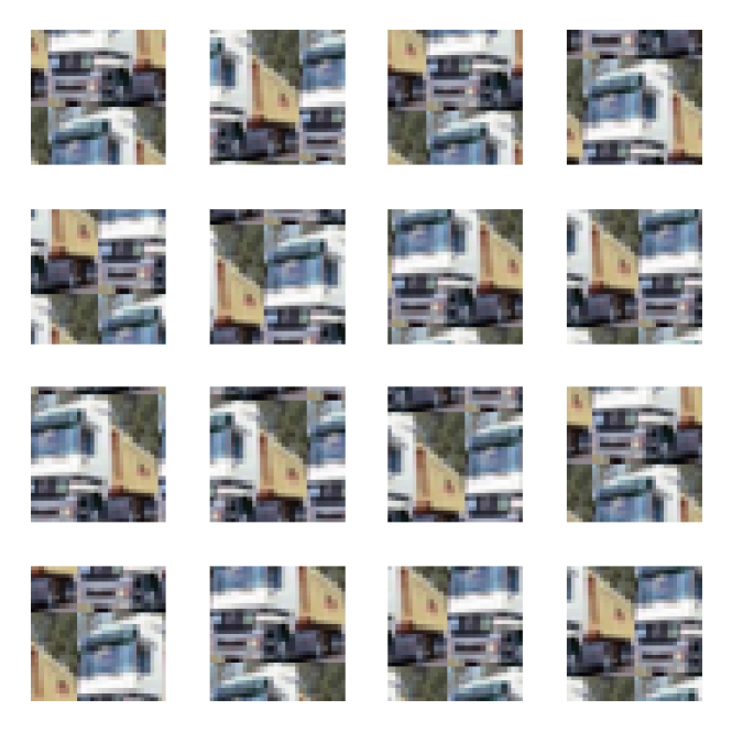
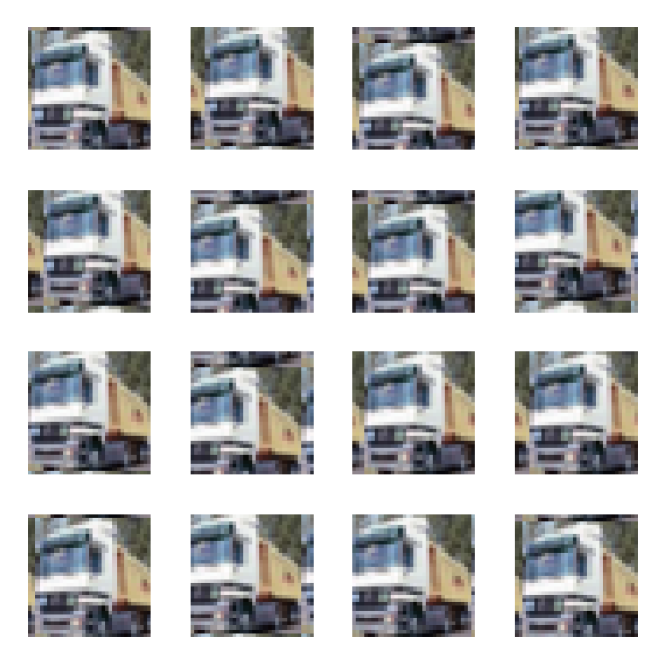
In this section, we introduce a new operation called Local Average Pooling (LAP). As discussed in the introduction, full translation data augmentation may create unrealistic images. A natural idea is to do local translation data augmentation, i.e., restricting the distance of translation. More specifically, we only allow translation operations (cf. Section 3.3) for where is a parameter to control the amount of allowed translation. With a proper choice of the parameter , translation data augmentation will not create unrealistic images (cf. Figure 1). However, naive local translation data augmentation is computationally infeasible for kernel methods, even for moderate choice of . To remedy this issue, in this section we introduce LAP, which is inspired by the connection between full translation data augmentation and GAP on CNN-GP and CNTK. Here, for simplicity, we assume and derive the formula only for CNTK. Our formula can be generalized to CNN-GP in a straightforward manner.
Recall that for two given images and , without GAP, the formula for output of CNTK is . With GAP, the formula for output of CNTK is
With circular padding, the formula can be rewritten as
which is again equal to
We ignore the scaling factor since it plays no role in kernel regression.
Now we consider restricted translation operations with and derive the formula for LAP. Assuming circular padding, we have
| (1) |
Now we have derived the formula for LAP, which is the RHS of Equation 1. Notice that the formula in the RHS of Equation 1 is a well-defined quantity for all padding schemes. In particular, assuming zero padding, when , LAP is equivalent to GAP. When , LAP is equivalent to no pooling layer. Another advantage of LAP is that it does not incur any extra computational cost, since the formula in Equation 1 can be rewritten as
where each entry in the weight tensor can be calculated in constant time.
Note that the GAP operation in CNN-GP and CNTK corresponds to the GAP layer in CNNs. Here we observe that the following box blur layer corresponds to LAP in CNNs. Box blur layer (BBlur) is a function such that
This is in fact the standard average pooling layer with pooling size and stride . We prove the equivalence between LAP and box blur layer in Appendix C. In Section 6.3, we verify the effectiveness of BBlur on CNNs via experiments.
6 Experiments
In this section we present our empirical findings on CIFAR-10 (Krizhevsky, 2009) and Fashion-MNIST (Xiao et al., 2017).
Experimental Setup.
For both CIFAR-10 and Fashion-MNIST we use the full training set and report the test accuracy on the full test set. Throughout this section we only consider convolutional filters with stride and no dilation. In the convolutional layers in CNTK and CNN-GP, we use zero padding with pad size to ensure the input of each layer has the same size. We use zero padding for LAP throughout the experiment. We perform standard preprocessing (mean subtraction and standard deviation division) for all images.
In all experiments, we perform kernel ridge regression to utilize the calculated kernel values333We also tried kernel SVM but found it significantly degrading the performance, and thus do not include the results.. We normalize the kernel matrices so that all diagonal entries are ones. Equivalently, we ensure all features have unit norm in RKHS. Since the resulting kernel matrices are usually ill-conditioned, we set the regularization term , to make inverting kernel matrices numerically stable. We use one-hot encodings of the labels as regression targets. We use scipy.linalg.solve to solve the corresponding kernel ridge regression problem.
The kernel value of CNTK and CNN-GP are calculated using the CuPy package. We write native CUDA codes to speed up the calculation of the kernel values. All experiments are performed on Amazon Web Services (AWS), using (possibly multiple) NVIDIA Tesla V100 GPUs. For efficiency considerations, all kernel values are computed with 32-bit precision.
One unique advantage of the dynamic programming algorithm for calculating CNTK and CNN-GP is that we do not need repeat experiments for, say, different values of in LAP and different depths. With our highly-optimized native CUDA codes, we spend roughly 1,000 GPU hours on calculating all kernel values for each dataset.
6.1 Ablation Study on CIFAR-10 and Fashion-MNIST
We perform experiments to study the effect of different values of the parameter in LAP and horizontal flip data argumentation on CNTK and CNN-GP. For experiments in this section we set the bias term in CNTK and CNN-GP to be (cf. Section A). We use the same architecture for CNTK and CNN-GP as in Arora et al. (2019). I.e., we stack multiple convolutional layers before the final pooling layer. We use to denote the number of convolutions layers, and in our experiments we set to be , , or , to study the effect of depth on CNTK and CNN-GP. For CIFAR-10, we set the parameter in LAP to be , while for Fashion-MNIST we set the parameter in LAP to be . Notice that when for CIFAR-10 or for Fashion-MNIST, LAP is equivalent to GAP, and when , LAP is equivalent to no pooling layer. Results on CIFAR-10 are reported in Tables 1 and 2, and results on Fashion-MNIST are reported in Tables 3 and 4. In each table, for each combination of and , the first number is the test accuracy without horizontal flip data augmentation (in percentage), and the second number (in parentheses) is the test accuracy with horizontal flip data augmentation.
| 0 | ||||
|---|---|---|---|---|
| 4 | ||||
| 8 | ||||
| 12 | ||||
| 16 | ||||
| 20 | ||||
| 24 | ||||
| 28 | ||||
| 32 |
| 0 | ||||
|---|---|---|---|---|
| 4 | ||||
| 8 | ||||
| 12 | ||||
| 16 | ||||
| 20 | ||||
| 24 | ||||
| 28 | ||||
| 32 |
| 0 | ||||
|---|---|---|---|---|
| 4 | ||||
| 8 | ||||
| 12 | ||||
| 16 | ||||
| 20 | ||||
| 24 | ||||
| 28 |
| 0 | ||||
|---|---|---|---|---|
| 4 | ||||
| 8 | ||||
| 12 | ||||
| 16 | ||||
| 20 | ||||
| 24 | ||||
| 28 |
We made the following observations regarding our experimental results.
-
•
LAP with a proper choice of the parameter significantly improves the performance of CNTK and CNN-GP. On CIFAR-10, the best-performing value of is or , while on Fashion-MNIST the best-performing value of is . We suspect this difference is due to the nature of the two datasets: CIFAR-10 contains real-life images and thus allow more translation, while Fashion-MNIST contains images with centered clothes and thus allow less translation. For both datasets, the best-performing value of is consistent across all settings (depth, CNTK or CNN-GP) that we have considered.
-
•
Horizontal flip data augmentation is less effective on Fashion-MNIST than on CIFAR-10. There are two possible explanations for this phenomenon. First, most images in Fashion-MNIST are nearly horizontally symmetric (e.g., T-shirts and bags). Second, CNTK and CNN-GP have already achieved a relatively high accuracy on Fashion-MNIST, and thus it is reasonable for horizontal flip data augmentation to be less effective on this dataset.
-
•
Finally, for CNTK, when (no pooling layer) and (GAP) our reported test accuracies are close to those in Arora et al. (2019) on CIFAR-10. For CNN-GP, when (no pooling layer) our reported test accuracies are close to those in Novak et al. (2019) on CIFAR-10 and Fashion-MNIST. This suggests that we have reproduced previous reported results.
6.2 Improving Performance on CIFAR-10 via Additional Pre-processing
Finally, we explore another interesting question: what is the limit of non-deep-neural-network methods on CIFAR-10? To further improve the performance, we combine CNTK and CNN-GP with LAP, together with the previous best-performing non-deep-neural-network method Coates et al. (2011). Here we use the variant implemented in Recht et al. (2019)444https://github.com/modestyachts/nondeep. More specifically, we first sample 2048 random image patches with size from all training images. Then for the sampled images patches, we subtract the mean of the patches, then normalize them to have unit norm, and finally perform ZCA transformation to the resulting patches. We use the resulting patches as 2048 filters of a convolutional layer with kernel size , stride and no dilation or padding. For an input image , we use to denote the output of the convolutional layer. As in the implementation in Recht et al. (2019), we use and as the input feature for CNTK and CNN-GP. Here we fix as in Recht et al. (2019), and set the bias term in CNTK and CNN-GP to be , which is the filter size used in CNTK and CNN-GP. To make the equivariant under horizontal flip (cf. Defintion 4.1), for each image patch, we horizontally flip it and add the flipped patch into the convolutional layer as a new filter. Thus, for an input CIFAR-10 image of size , the dimension of the output feature is . To isolate the effect of randomness in the choices of the image patches, we fix the random seed to be 0 throughout the experiment. In this experiment, we set the value of the parameter in LAP to be to avoid small and large values of . The results are reported in Tables 5 and 6. In each table, for each combination of and , the first number is the test accuracy without horizontal flip data augmentation (in percentage), and the second number (in parentheses) is the test accuracy with horizontal flip data augmentation (again in percentage).
| 4 | ||||
|---|---|---|---|---|
| 8 | ||||
| 12 | ||||
| 16 | ||||
| 20 |
| 4 | ||||
|---|---|---|---|---|
| 8 | ||||
| 12 | ||||
| 16 | ||||
| 20 |
From our experimental results, it is evident that combining CNTK or CNN-GP with additional pre-processing can significantly improve upon the performance of using solely CNTK or CNN-GP, and that of using solely the approach in Coates et al. (2011). Previously, it has been reported in Recht et al. (2019) that using solely the approach in Coates et al. (2011) (together with appropriate pooling layer) can only achieve a test accuracy of 84.2% using 256, 000 image patches, or 83.3% using 32, 000 image patches. Even with the help of horizontal flip data augmentation, the approach in Coates et al. (2011) can only achieve a test accuracy of 85.6% using 256, 000 image patches, or 85.0% using 32, 000 image patches. Here we use significantly less image patches (only 2048) but achieve a much better performance, with the help of CNTK and CNN-GP. In particular, we achieve a performance of 88.92% on CIFAR-10, matching the performance of AlexNet on the same dataset. In the setting reported in Coates et al. (2011), increasing the number of sampled image patches will further improve the performance. Here we also conjecture that in our setting, further increasing the number of sampled image patches can improve the performance and get close to modern CNNs. However, due the limitation on computational resources, we leave exploring the effect of number of sampled image patches as a future research direction.
6.3 Experiments on CNN with BBlur
In Figure 2, we verify the effectiveness of BBlur on a 10-layer CNN (with Batch Normalization) on CIFAR-10. The setting of this experiment is reported in Appendix D. Our network structure has no pooling layer except for the BBlur layer before the final fully-connected layer. The fully-connected layer is fixed during the training. Our experiment illustrates that even with a fixed final FC layer, using GAP could improve the performance of CNN, and challenges the conjecture that GAP reduces the number of parameters in the last fully-connected layer and thus avoids overfitting. Our experiments also show that BBlur with appropriate choice of achieves better performance than GAP.
7 Conclusion
In this paper, inspired by the connection between full translation data augmentation and GAP, we derive a new operation, LAP, on CNTK and CNN-GP, which consistently improves the performance on image classification tasks. Combining CNN-GP with LAP and the pre-processing technique proposed by Coates et al. (2011), the resulting kernel achieves 89% accuracy on CIFAR-10, matching the performance of AlexNet and is the strongest classifier that is not a trained neural network.
Here we list a few future research directions. Is that possible to combine more modern techniques on CNN, such as batch normalization and residual layers, with CNTK or CNN-GP, to further improve the performance? Moreover, it is an interesting direction to study other components in modern CNNs through the lens of CNTK and CNN-GP.
Acknowledgements
S. Arora, W. Hu, Z. Li and D. Yu are supported by NSF, ONR, Simons Foundation, Schmidt Foundation, Amazon Research, DARPA and SRC. S. S. Du is supported by National Science Foundation (Grant No. DMS-1638352) and the Infosys Membership. R. Salakhutdinov and R. Wang are supported in part by NSF IIS-1763562, Office of Naval Research grant N000141812861, and Nvidia NVAIL award. Part of this work was done while R. Wang was visiting Princeton University. The authors would like to thank Amazon Web Services for providing compute time for the experiments in this paper.
References
- Allen-Zhu et al. (2018) Zeyuan Allen-Zhu, Yuanzhi Li, and Zhao Song. A convergence theory for deep learning via over-parameterization. arXiv preprint arXiv:1811.03962, 2018.
- Arora et al. (2019) Sanjeev Arora, Simon S Du, Wei Hu, Zhiyuan Li, Ruslan Salakhutdinov, and Ruosong Wang. On exact computation with an infinitely wide neural net. arXiv preprint arXiv:1904.11955, 2019.
- Chapelle et al. (2001) Olivier Chapelle, Jason Weston, Léon Bottou, and Vladimir Vapnik. Vicinal risk minimization. In Advances in neural information processing systems, pages 416–422, 2001.
- Chen et al. (2019) Shuxiao Chen, Edgar Dobriban, and Jane H Lee. Invariance reduces variance: Understanding data augmentation in deep learning and beyond. arXiv preprint arXiv:1907.10905, 2019.
- Coates et al. (2011) Adam Coates, Andrew Ng, and Honglak Lee. An analysis of single-layer networks in unsupervised feature learning. In Proceedings of the fourteenth international conference on artificial intelligence and statistics, pages 215–223, 2011.
- Dao et al. (2018) Tri Dao, Albert Gu, Alexander J Ratner, Virginia Smith, Christopher De Sa, and Christopher Ré. A kernel theory of modern data augmentation. arXiv preprint arXiv:1803.06084, 2018.
- Du et al. (2018) Simon S Du, Jason D Lee, Haochuan Li, Liwei Wang, and Xiyu Zhai. Gradient descent finds global minima of deep neural networks. arXiv preprint arXiv:1811.03804, 2018.
- Du et al. (2019a) Simon S. Du, Kangcheng Hou, Barnabás Póczos, Ruslan Salakhutdinov, Ruosong Wang, and Keyulu Xu. Graph neural tangent kernel: Fusing graph neural networks with graph kernels. ArXiv, abs/1905.13192, 2019a.
- Du et al. (2019b) Simon S. Du, Xiyu Zhai, Barnabas Poczos, and Aarti Singh. Gradient descent provably optimizes over-parameterized neural networks. In International Conference on Learning Representations, 2019b.
- Garriga-Alonso et al. (2019) Adrià Garriga-Alonso, Carl Edward Rasmussen, and Laurence Aitchison. Deep convolutional networks as shallow gaussian processes. In International Conference on Learning Representations, 2019. URL https://openreview.net/forum?id=Bklfsi0cKm.
- He et al. (2016) Kaiming He, Xiangyu Zhang, Shaoqing Ren, and Jian Sun. Deep residual learning for image recognition. In Proceedings of the IEEE conference on computer vision and pattern recognition, pages 770–778, 2016.
- Huang et al. (2017) Gao Huang, Zhuang Liu, Laurens Van Der Maaten, and Kilian Q Weinberger. Densely connected convolutional networks. In Proceedings of the IEEE conference on computer vision and pattern recognition, pages 4700–4708, 2017.
- Jacot et al. (2018) Arthur Jacot, Franck Gabriel, and Clément Hongler. Neural tangent kernel: Convergence and generalization in neural networks. arXiv preprint arXiv:1806.07572, 2018.
- Krizhevsky (2009) Alex Krizhevsky. Learning multiple layers of features from tiny images. 2009.
- Krizhevsky et al. (2012) Alex Krizhevsky, Ilya Sutskever, and Geoffrey E Hinton. Imagenet classification with deep convolutional neural networks. In Advances in neural information processing systems, pages 1097–1105, 2012.
- Lee et al. (2018) Jaehoon Lee, Jascha Sohl-dickstein, Jeffrey Pennington, Roman Novak, Sam Schoenholz, and Yasaman Bahri. Deep neural networks as gaussian processes. In International Conference on Learning Representations, 2018. URL https://openreview.net/forum?id=B1EA-M-0Z.
- Li and Liang (2018) Yuanzhi Li and Yingyu Liang. Learning overparameterized neural networks via stochastic gradient descent on structured data. arXiv preprint arXiv:1808.01204, 2018.
- Lin et al. (2013) Min Lin, Qiang Chen, and Shuicheng Yan. Network in network. arXiv preprint arXiv:1312.4400, 2013.
- Matthews et al. (2018) Alexander G de G Matthews, Mark Rowland, Jiri Hron, Richard E Turner, and Zoubin Ghahramani. Gaussian process behaviour in wide deep neural networks. arXiv preprint arXiv:1804.11271, 2018.
- Neal (1996) Radford M Neal. Priors for infinite networks. In Bayesian Learning for Neural Networks, pages 29–53. Springer, 1996.
- Novak et al. (2019) Roman Novak, Lechao Xiao, Yasaman Bahri, Jaehoon Lee, Greg Yang, Daniel A. Abolafia, Jeffrey Pennington, and Jascha Sohl-dickstein. Bayesian deep convolutional networks with many channels are gaussian processes. In International Conference on Learning Representations, 2019. URL https://openreview.net/forum?id=B1g30j0qF7.
- Recht et al. (2019) Benjamin Recht, Rebecca Roelofs, Ludwig Schmidt, and Vaishaal Shankar. Do imagenet classifiers generalize to imagenet? arXiv preprint arXiv:1902.10811, 2019.
- Schölkopf et al. (1996) Bernhard Schölkopf, Chris Burges, and Vladimir Vapnik. Incorporating invariances in support vector learning machines. In International Conference on Artificial Neural Networks, pages 47–52. Springer, 1996.
- Sietsma and Dow (1991) Jocelyn Sietsma and Robert JF Dow. Creating artificial neural networks that generalize. Neural networks, 4(1):67–79, 1991.
- Springenberg et al. (2014) Jost Tobias Springenberg, Alexey Dosovitskiy, Thomas Brox, and Martin Riedmiller. Striving for simplicity: The all convolutional net. arXiv preprint arXiv:1412.6806, 2014.
- Xiao et al. (2017) Han Xiao, Kashif Rasul, and Roland Vollgraf. Fashion-mnist: a novel image dataset for benchmarking machine learning algorithms, 2017.
- Yang (2019) Greg Yang. Scaling limits of wide neural networks with weight sharing: Gaussian process behavior, gradient independence, and neural tangent kernel derivation. arXiv preprint arXiv:1902.04760, 2019.
- Zou et al. (2018) Difan Zou, Yuan Cao, Dongruo Zhou, and Quanquan Gu. Stochastic gradient descent optimizes over-parameterized deep ReLU networks. arXiv preprint arXiv:1811.08888, 2018.
Appendix A Formal Definitions of CNN, CNN-GP and CNTK
In this section we use the following additional notations. Let be the identity matrix, and . Let be an indicator vector with -th entry being and other entries being , and let denote the all-one vector. We use to denote the pointwise product and to denote the tensor product. We use to transform a vector to a diagonal matrix. We use to denote the activation function, such as the rectified linear unit (ReLU) function: , and to denote the derivative of . Moreover, is a fixed constant. Denote by the Gaussian distribution with mean and covariance .
We first define the convolution operation. For a convolutional filter and an image , the convolution operator is defined as
| (2) |
Here the precise definition of and depends on the padding scheme (cf. Section 3.2). Notice that in Equation 2, the value of depends on . Thus, for , we define
Now we formally define CNN, CNN-GP and CNTK.
CNN.
-
•
Let be the input image where is the initial number of channels.
-
•
For , , the intermediate outputs are defined as
where each is a filter with Gaussian initialization, is a bias term with Gaussian initialization, and is the scaling factor for the bias term.
CNN-GP and CNTK.
-
•
For , , define
-
•
For ,
-
–
For , define
-
–
For , define
(3) (4) -
–
For , define
-
–
Note that the definition of and share similar patterns as their NTK counterparts [Jacot et al., 2018]. The only difference is that we have one more step, taking the trace over patches. This step represents the convolution operation in the corresponding CNN. Now we can define the kernel value recursively.
-
1.
First, we define .
-
2.
For and , we define
-
3.
Finally, define
Appendix B Additional Definitions and Proof of Theorem 4.1
Definition B.1 (Group of Operators).
is a group of operators, if and only if
-
1.
Each element is an operator: ;
-
2.
, where is defined as .
-
3.
, such that , .
-
4.
, , such that . We say is the inverse of , namely, .
Proof of Theorem 4.1.
Since we assume and are invertible, both and are uniquely defined. Now we claim is equal to for all .
By the equivariance of under , for all and ,
Note that is defined as the unique solution of .
Similarly, we have
∎
Appendix C Equivalence Between LAP and Box Blur Layer.
For a CNN with a box blur layer before the final fully-connected layer, the final output is defined as , where , and is the weight of the last fully-connected layer.
Now we establish the equivalence between BBlur and LAP on CNTK. The equivalence on CNN-GP can be derived similarly. Let be the CNTK kernel of . Since BBlur is just a linear operation, we have
By the formula of the output kernel value for CNTK without GAP, we obtain
Appendix D Setting of the Experiment in Section 6.3
The total number of training epochs is 80, and the learning rate is 0.1 initially, decayed by 10 at epoch 40 and 60 respectively. The momentum is 0.9 and the weight decay factor is 0.0005. In Figure 2, the blue line reports the average test accuracy of the last 10 epochs, while the red line reports the best test accuracy of the total 80 epochs. Each experiment is repeated for 3 times. We use circular padding for both convolutional layers and the BBlur layer. The last data point with largest -coordinate reported in Figure 2 corresponds to GAP.