Superfield Component Decompositions and the Scan for Prepotential Supermultiplets in 10D Superspaces
S. James Gates, Jr.111sylvester-gates@brown.edu,a,b, Yangrui Hu222yangrui-hu@brown.edua,b, and S.-N. Hazel Mak333sze-ning-mak@brown.edua,b
aBrown Theoretical Physics Center,
Box S, 340 Brook Street, Barus Hall,
Providence, RI 02912-1843, USA
bDepartment of Physics, Brown University,
Box 1843, 182 Hope Street, Barus & Holley,
Providence, RI 02912, USA
ABSTRACT
The first complete and explicit SO(1,9) Lorentz descriptions of all component fields contained in the , A, and B unconstrained scalar 10D superfields are presented. These are made possible by a discovery of the dependence of the superfield component expansion on the branching rules of irreducible representations in one ordinary Lie algebra into one of its Lie subalgebras. Adinkra graphs for ten dimensional superspaces are defined for the first time, whose nodes depict spin bundle representations of SO(1,9). A consequential deliverable of this advance is it provides the first explicit, in terms of component fields, examples of all the off-shell 10D Nordström SG theories relevant to string theory, without off-shell central charges that are reducible but with finite numbers of fields. An analogue of Breitenlohner’s approach is implemented to scan for superfields that contain graviton(s) and gravitino(s), which are the candidates for the superconformal prepotential superfields of 10D off-shell supergravity theories and Yang-Mills theories.
PACS: 11.30.Pb, 12.60.Jv
Keywords: supersymmetry, super gauge theories, supergravity, superfield, off-shell, branching rules
1 Introduction
On the basis of superspace geometry, recently a study [?] of the problem of describing scalar gravitation at the linearized level within the context of eleven and ten dimensional superspaces was completed. The results of this effort showed with regards to supergeometical concepts there were no significant differences (nor more importantly obstructions) between this problem in the high dimensional superspaces than in a four dimensional superspace. Though one important distinction was noted… there is a long standing lack of a general theory of irreducibility in the area of scalar superfield representations. Related to this is the problem of defining a superconformal multiplet in these regimes. We were thus re-energized to look at these problems.
One of the longest unsolved problems in the study of supersymmetry is the fact that an irreducible off-shell formulation containing a finite number of component fields for the ten dimensional (along with the extended and eleven dimensional ones) supergravity multiplet has not been presented. This statement accurately describes the current state-of-the-art of the field well after thirty years since it began. An even simpler problem is to give a detailed component level presentation of a reducible off-shell formulation explicitly showing a finite number of component fields. It is the purpose of this work to report on new techniques for the second of these problems. Though more work will need to be done to find these.
In this work we have new developed techniques, both algorithmic and analytical, that allow the first complete and explicit SO(1,9) Lorentz descriptions of all component fields contained in 10D, , , and unconstrained scalar superfields. They form the maximal reducible and relevant supermultiplets. For the case of the theory, our results agree with the first report on this topic [?] given by Bergshoeff and de Roo. These authors took as their starting point an analysis of the “supercurrent corresponding to the supersymmetic Maxwell theory in ten dimensions.” An approach of this type is tied to making an initial assumption about the dynamics of some supersymmetrical system, i.e. the choice of the energy-momentum tensor.
The previous sentence illustrates a peculiarity of the study of spacetime supersymmetry in comparison to other symmetries. Namely, almost all studies of the representations of spacetime supersymmetry take as a starting a set of assumptions related to some dynamic system. This is shared by no other symmetry known to these authors. Thus, there is a possibility by exploring avenues that depart from dynamical assumptions, a resolution to the puzzles may be found.
We will present the maximal reducible relevant representations of supergravity in 10D related to unconstrained scalar superfields by “tensoring” them with different representations of the SO(1,9) Lorentz group and search for graviton(s) and gravitino(s). To achieve this goal, we borrow Breitenlohner’s approach [?], which gave the first off-shell 4D, supergravity description. It utilized the known off-shell structure of the 4D, vector supermultiplet . Since the structure of off-shell supermultiplets in ten dimensions is poorly understood, we implement the approach of Breitenlohner by use of a 10D scalar superfield in place of the vector supermultiplet. This will ensure an off-shell supersymmetry realization.
There are three guiding principles implied by the Breitenlohner appoaoch that
are implemented in our discussion, use: (a.) no dynamical assumptions in
the derivation of representation
theory results,
(b.) only conventional Wess-Zumino superspaces, and
(c.) superfields that admit an unconstrained prepotential formulation.
These are the principles that allowed for the complete off-shell superspace descriptions of
supergravity in 4D, = 1 theories. Our current investigation looks to extend these
beyond the lower dimensional context and into the domain of the 10D theories. The operational steps to implement the paradigm of the approach include
(a.) identify an appropriate scalar supermultipet free of dynamical
assumptions with regards to the
closure of the superalgebra,
(b.) tensor the scalar supermultiplet with representations of
the
Lorentz algebra, and
(c.) among the results found by the
tensoring operation, search
for components that align with the Lorentz representations of
conformal graviton and gravitino.
As this approach is independent of any assumptions about dynamics of the component fields contained in supermultiplets, there should be an expectation of differences in comparison with any past results derived from an analysis where dynamics are built into a conceptual foundation.
It is known that when a supersymmetrical theory is expressed in terms of prepotentials, the reasons for many unexpected enhancement of vanishing quantum corrections become obvious. So we restrict our considerations to formulations that are consistent with prepotentials. This further restricts our considerations to solely theories that demonstrate an absence of “off-shell central charges” [?,?,?,?,?].
The keys to our progress in this realm are higher dimensional adinkras (built upon the well established foundation of one dimensional ones [?,?,?,?,?,?,?,?,?,?,?,?,?]) and advanced computational tools. These techniques are derived via properties of representation theory and thus are independent of assumptions about dynamics.
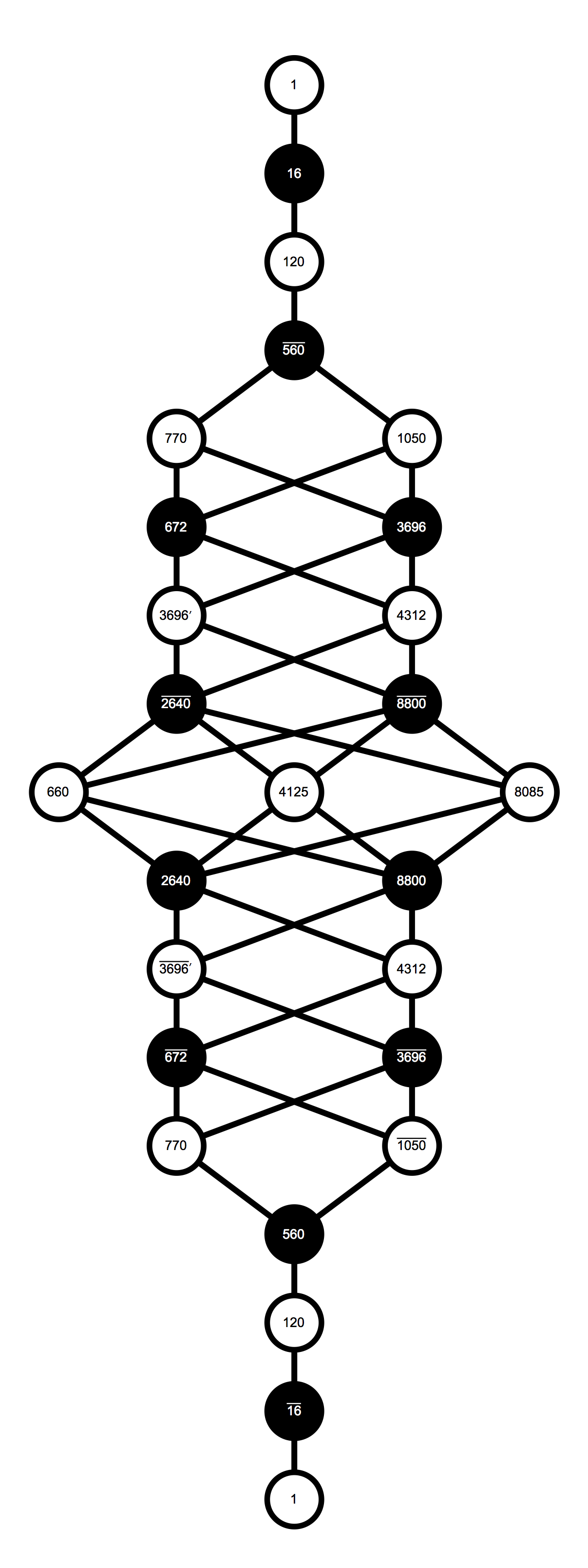
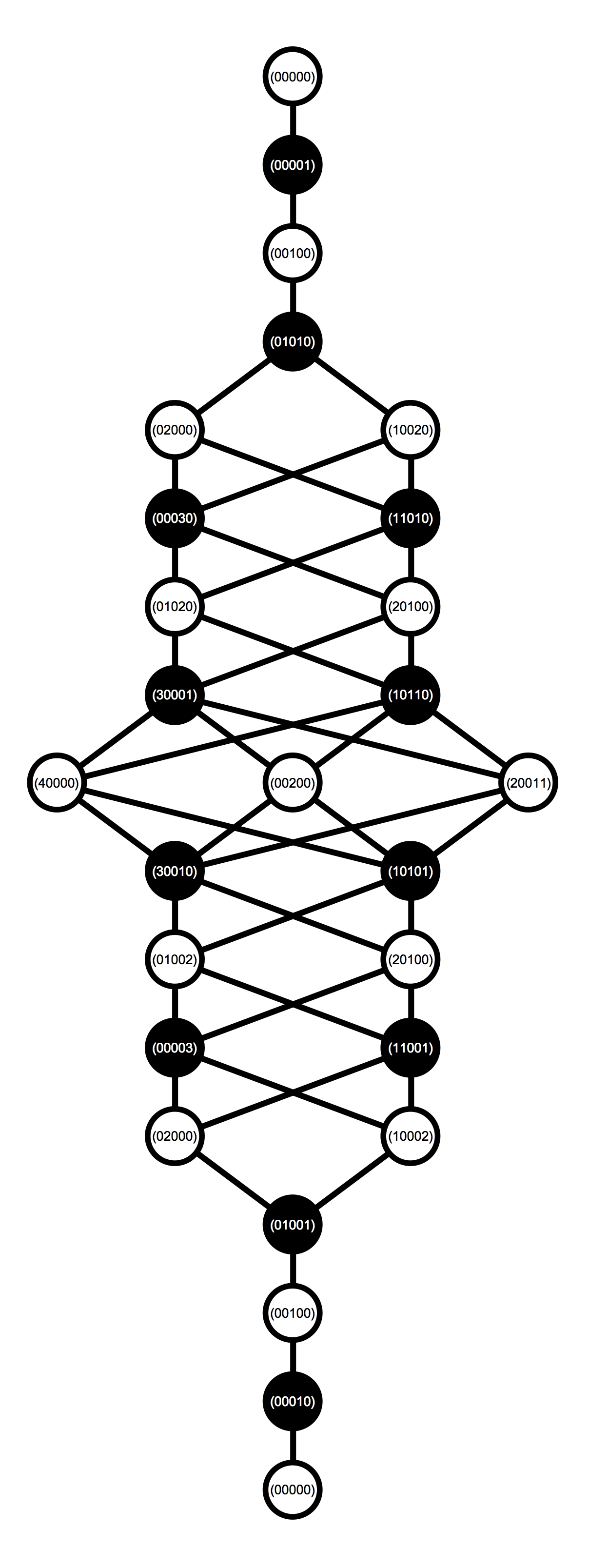
For the first of these keys, we have built upon efforts that began in the work of [?] wherein the first two images shown in Figure 1.1 were presented.
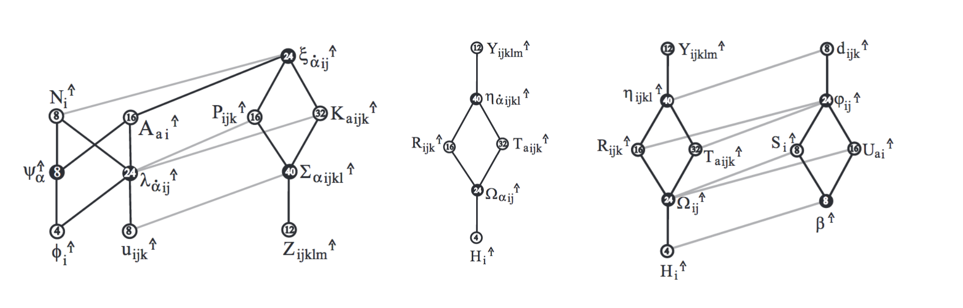
More recently Faux [?] introduced the third image in Figure 1.1. All the supermultiplets depicted are “off-shell,” i.e. the closure of the supersymmetry algebra does not require the use of the equation of motion for any component field.
The graphs from [?] are among the first in the literature where the individual nodes of one dimensional adinkras are “aggregated” together into structures that carry non-trivial representations of the Lorentz group. Furthermore, the links in this class of diagrams are also “aggregations” of the links that appear in the one dimensional adinkras. Both of these attributes pointed to the possibility of constructing adinkras in higher dimensions where both nodes and links can be regarded as aggregations of the one-dimensional concepts.
The important principle established by the explicit demonstration of these graphs is that it is a priori possible to construct adinkras in greater than one dimensional contexts. This is not, however, an “organic” constructive process. Namely, these structures were obtained by first completing a component-level analytical construction of the supermultiplet. An “organic” process would dispense with any component-level lead-in. Instead on the basis of a set of principles and tools, there should be a way to construct such adinkras in higher dimensions. This is the primary goal of this current work.
Also on the analytical side, our efforts will build upon a class of works [?,?,?] wherein the concept of the “Tableaux calculus” was discussed by Howe, Stelle, and Townsend. To our knowledge, these were the first works that explicitly discussed the use of Young Tableaux as applied to problems in the representation theory of spacetime supersymmetry.
The supermultiplets illustrated in Figure 1.1 are constrained, i.e. subject to supercovariant derivative differential equations. This is also the case of the works by Howe, Stelle, and Townsend. In particular, these authors proposed to use Young Tableaux that are associated with the superspace covariant derivative operators acting on constrained supermultiplets. The concept of associating the superspace covariant derivative operators with Tableaux images will be important in our work. In our exploration, we also find it useful to utilize the more conventional class of Tableaux that are associated with bosonic Lorentz indices carried by fields. We will call the former of these Young Tableaux “fermionic Young Tableaux” (FYT) while distinguishing the latter by the term “bosonic Young Tableaux” (BYT). An important distinction of our work is the supermultiplets are unconstrained.
Our work is also a beneficiary of a report undertaken by N. Yamatsu [?] who presented results for grand unified model-building based on finite-dimensional Lie algebras. In this work, the reader can find results for projection matrices and branching rules between Lie algebras and their subalgebras up to high ranks, as well as Dynkin labels and Weyl dimensional formulae of irreducible representations, and much more. The results we have explicitly called out in the last sentence have proven to be particularly useful when applied to the SO(1,9) representation theory we consider. It is of historical note, that the work by Yamatsu falls among the path of earlier explorations [?,?,?].
The final enabling tool for our work is based on algorithmic efficiency and here the work by Feger and Kephart [?] played an important role. These authors developed and presented a Mathematica application - Lie Algebras and Representation Theory (LieART) which carries out computations typically occurring in the context of Lie algebras and representation theory. This provides a robust algorithm that enables the study of weight systems. One of its features that enhances its efficiency is the use of Dynkin labels for irreducible representations. It is thus ideal for specializing to SO(1,9) representation theory.
We organize this current paper in the manner described below. In Chapter two we discuss the numbers of independent bosonic and fermionic components in a scalar superfield. Chapter three is a transitional one where we review the expansion of a real scalar superfield in 4D, theory and introduce the higher dimensional adinkra technology. In Chapter four, we present the component decomposition result of the scalar superfield in 10D, theory. Two different approaches that lead to the same result are presented. One we call the “handicraft approach,444The term “handicraft approach” comes for P. van Nieuwenhuizen who coined it to refer to a mathematical “Rube Goldberg” type of approach that nevertheless yields a correct result in the context of supersymmetry calculations. ” where we introduce Bosonic and Fermionic Young Tableaux. The other is the application of branching rules, the restrictions of representations from a Lie algebra to one of its subalgebra . The complete ten dimensional adinkra is drawn. In Chapter five, we start from the well-studied off-shell description of 4D, supergravity established by Breitenlohner and show how to apply his idea to carry out constructions of candidates for the prepotential and Yang-Mills supermultiplets in 10D, theory. In Chapter six, we present the methodology and results of constructing the 10D, A scalar superfield from the 10D, scalar superfield, as well as the discussion of the search of prepotential supermultiplet in Type IIA superspace. The ten dimensional IIA adinkra diagram is shown at low orders. However, its complete structure is given in the form of a list of the component field representations it contains. These same steps are repeated in chapter seven that gives the methodology and explicit decomposition results as well as the discussion of constructing prepotential supermultiplet in Type IIB superspace. The ten dimensional IIB adinkra diagram is also shown at low orders.
We follow the presentation of our work with conclusions, three appendices, and the bibliography. The first appendix gives detailed discussions about chiral and vector supermultiplets obtained from 4D, = 1 unconstrained scalar superfield. The second appendix contains tables of SO(1,9) representations drawn from the work of Yamatsu. The third appendix presents the results of “tensoring” low order bosonic representations of SO(1,9) with the basic unconstrained 10D, = 1 scalar superfield. Finally, the fourth appendix presents the results of “tensoring” low order fermionic representations of SO(1,9) with the basic unconstrained 10D, = 1 scalar superfield.
2 Superfield Diophantine Considerations
Via the use of simple toroidal compactification, one can count the numbers of independent bosonic and fermionic component fields that occur in a scalar superfield. As a fermionic coordinate cannot be squared, this means in the Grassmann coordinate expansion of a superfield, any one specific fermionic coordinate can only occur to the zeroth power or the first power. As component fields occur as coefficients of monomials in superspace Grassmann coordinates, counting the latter is the same as the former… as long as the superfield is not subject to any spinorial “supercovariant derivative” constraints.
Each higher dimensional superspace with bosonic dimensions, for purposes of counting is equivalent to some value of , where is the number of independent equivalent real one-dimensional fermionic coordinates on which the superfield depends. The total number of independent monomials is given by . Next, to count the total number of bosonic components in the scalar superfield, we simply divide by a factor of two. This same argument applies to the total number of fermionic components in the scalar superfield. Thus we have = = . A few cases are shown in the table below.
| 4 | 4 | 16 | 8 | 8 |
| 5 | 8 | 256 | 128 | 128 |
| 10 | 16 | 65,536 | 32,768 | 32,768 |
| 11 | 32 | 4,294,967,296 | 2,147,483,648 | 2,147,483,648 |
spacetime
While superfields easily provide a methodology for finding collections of component fields that are representations of spacetime supersymmetry, one thing that superfields do not yield so easily is a theory of the constraints that provides irreducible representations. For any constrained superfield, it must be the case that the number of component fields does not depend solely on the parameter . This is most certainly true for the maximally constrained and therefore minimal irreducible representations. This is illustrated by comparing the final two columns of the first three rows in Tables 1 and 2 that = = .
| 4D Minimal Off-Shell Supermultiplet | ||||
|---|---|---|---|---|
| = 1 Chiral | 4 | 8 | 4 | 4 |
| = 2 Vector | 8 | 128 | 8 | 8 |
| = 4 SG | 16 | 32,768 | 128 | 128 |
In this paper, we will decompose the 10D unconstrained scalar superfields into component fields that transform under the Lorentz group SO(1,9).
3 4D Scalar Superfield Decomposition
The off-shell four dimensional vector supermultiplet is well understood now to be a part of the unconstrained superfield as given below. In 4D, real superspace, the spinor index (the Greek index) on runs from 1 to 4, and we have 8 bosons and 8 fermions, as counted in Table 1. The expansion of a scalar superfield is
| (3.1) |
where , , , , and are bosonic component fields with 8 d.o.f.555We use the notation d.o.f to indicate “degrees of freedom.” in total; and are fermionic component fields with 8 d.o.f. in total. We will discuss this expansion result from different perspectives.
3.1 Group Theory Perspective
From the perspective of group theory, we can translate the scalar superfield decomposition problem to the irreducible decomposition problem of representations in . First, we can write the general expression of the expansion of a superfield
| (3.2) |
Due to the antisymmetric property of the Grassmann coordinates , the quantities , , , and have 4, 6, 4, and 1 degrees of freedom, respectively. They can be interpreted as representations of with 4, 6, 4, and 1 dimensions. We use level- to denote the monomial with s. The problem is reduced to do the irreducible decompositions of these representations and the results can be listed as
| (3.3) |
Note that level-4 and 3 are conjugate to level-0 and 1, respectively, while level-2 is self-conjugate. The conjugates of and are still and . Level-2 has two ’s666If one is exercising extra care, the ’s at level-2 are not identical. In fact, one of these corresponds to a scalar field while the other corresponds to a pseudoscalar. However, for our purposes, we can neglect this difference. This distinction is shown in Table 3 where the “count” is the same for both, but their projections to -matrices are distinct.. Although in the group theory context, only has one , here two ’s represent two different monomials as you will see shortly.
In order to distinguish between bosonic irreps and fermionic irreps, we color their dimensions: blue if bosonic and red if fermionic. In the rest of the paper, we will use these conventions.
Recall that in 4D, real superspace, we can create the covariant gamma matrices which are real matrices. The basis of the space of matrices over these spinors is summarized in Table 3.
| Basis | |||||
|---|---|---|---|---|---|
| Sym/Antisym | A | S | S | A | A |
| Count | 1 | 4 | 6 | 1 | 4 |
3.2 Graph Theory Perspective: Adinkra
From the perspective of graph theory, particularly adinkra diagrams, we can define a four dimensional adinkra based on Equation (3.3). First of all, the adinkra diagram carries information about component fields rather than monomials, so we need to translate Equation (3.3) to field variable language. Consider a variable with one upstairs spinor index and assign irrep to this field. What is the irrep corresponding to the variable with one downstairs spinor index ? Since
| (3.6) |
where is the spinor metric, the irrep of is still . Generally speaking, in 4D, = 1 real notation, the irreps corresponding to component fields are the same as their monomials.
Then we can use open nodes to denote bosonic component fields and put the dimensions of their corresponding irreps in the centers of the open nodes. For fermionic component fields, we use closed nodes with a similar convention for dimensionality. The level number represents the height assignment and it increases with height. Black edges connect nodes in adjacent levels and represent supersymmetric transformation operations on the component fields. We can also interpret the adinkra using the idea in [?] (i.e. adinkra nodes are the 0 limit of superfields), as illustrated in the following table.
| Level | Adinkra nodes | Component fields | Irrep(s) in |
|---|---|---|---|
| 0 | |||
| 1 | |||
| 2 | , , | , , | |
| 3 | |||
| 4 |
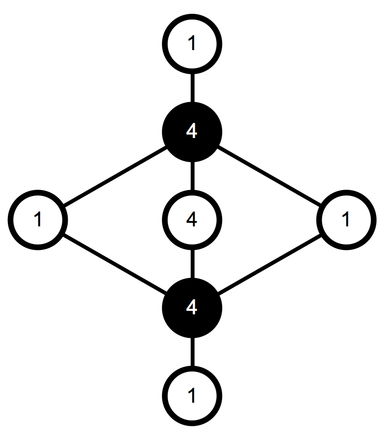
Since the physical d.o.f. of is , the height assignment describes the the physical d.o.f. of component fields as well. The corresponding adinkra diagram is Figure 3.1. The graph shows the “” bosonic component field at the lowest level, the “” fermionic field at level one, the “,” “,” and “” bosonic component fields at level two, the “” fermionic field at level three, and finally the “” bosonic component field at level four.
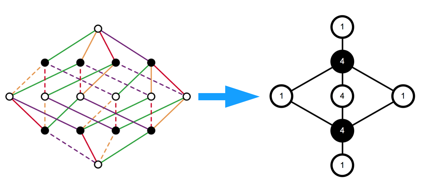
Since the 4D, = 1 theory can be truncated to a 1D, = 4 theory, we can discuss the relation between the 4D, = 1 adinkra and the 1D, = 4 adinkra as shown in Figure 3.2. The 1D, = 4 maximal supermultiplet and the corresponding adinkras are well-studied. The graph shown to the left graph in Figure 3.2 illustrates the 1D = 4 system.
By comparison, we see that starting from the 1D, = 4 adinkra, if we aggregate a set of bosons or fermions into a single node, then a set of corresponding links will be merged (we use black links to replace them), and thus emerges the 4D, = 1 adinkra. Of course, to reach this goal we must decide to enforce some rules. Four and only four black nodes are merged at the first and third levels. At the second level, the only merging choices are either one or four nodes as permitted in an “aggregated” node. From this procedure, although we have a large number of different 1D, adinkras, they all collapse into the same 4D, version. It is useful to also recall that the aggregation of nodes leads to “dimensional enhancement” [?,?,?] that allows the adinkra nodes to carry representations of the four dimensional Lorentz group.
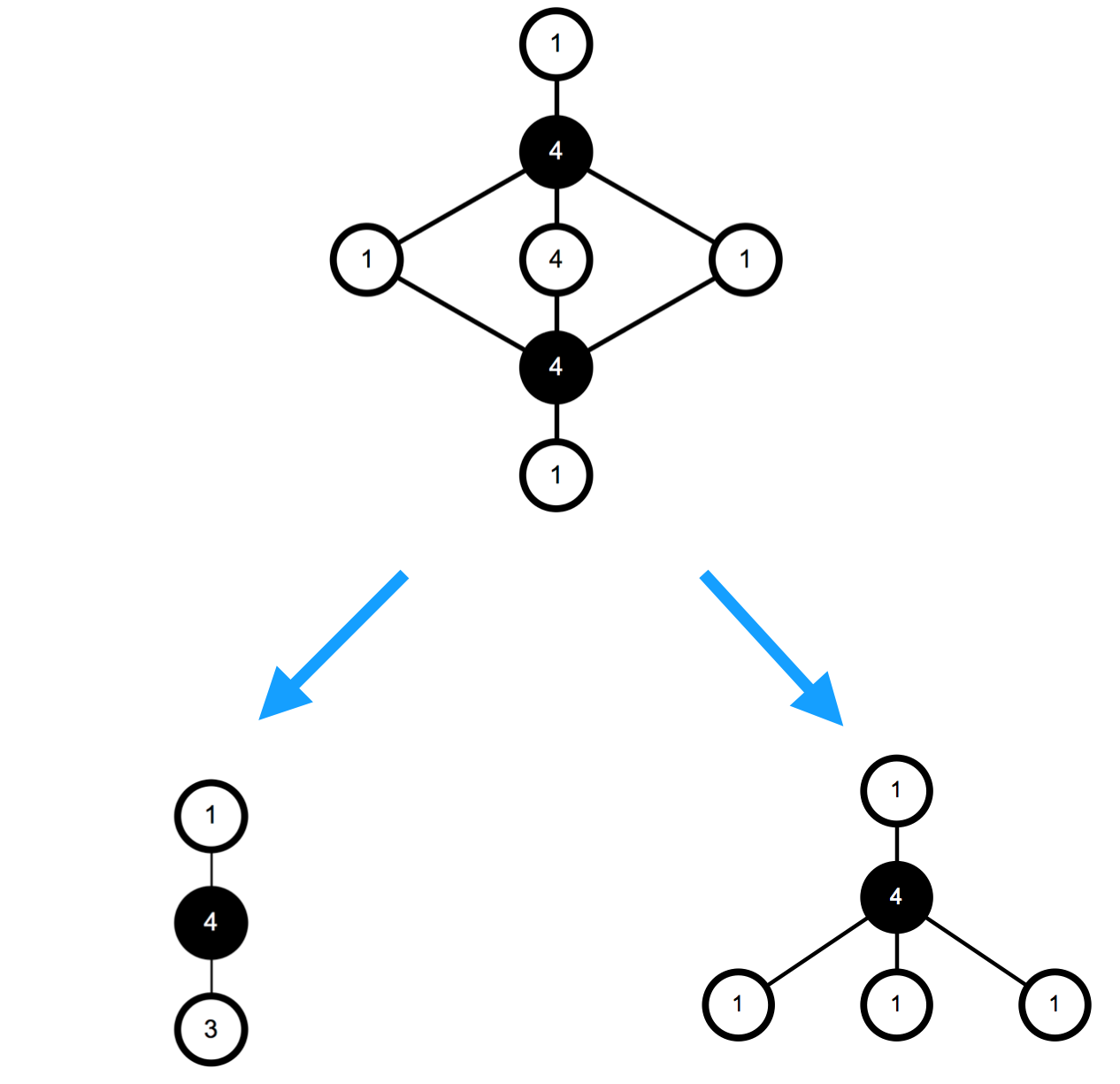
Before we leave this section, there is another relevant comment. Figure 3.1 provides a representation of the data needed to construct the component field description of the 4D, unconstrained superfield . However, this superfield is well known to provide a reducible representation of 4D, supersymmetry. The irreducible representations contained in are the two adinkra diagrams on the bottom of Figure 3.3.
It is useful to know one of the nodes at the lowest level of the bottom right graph in Figure 3.3 (i.e. chiral supermultiplet) must be regarded as the spacetime integral of a spin-0 field. The origin of this field was from the initial starting point as being one of the aggregated part of the “4” at the middle level of the adinkra. The bottom left graph in Figure 3.3 has nodes associated with the component fields of the vector supermultiplet where the gauge field is restricted to the Coulomb gauge. Refer to Appendix A for details.
In 4D, there is a comprehensive understanding of how to start with a reducible representation such as the real scalar superfield and “break” it apart into its irreducible components. However, the extension of such a procedure is totally unknown for the cases of 10D superfields.
For a general representation of spacetime supersymmetry, there is currently no understanding of how to carry out the process which has been accomplished in the realm of the 4D, = 1 supersymmetry. Resolving this class of problems in the realm of supersymmetric representation theory is a primary motivation for the adinkra approach to the study of superfields.
If we borrow the language of genetics, adinkras play the role of genomes for superfields. The problem of finding the irreducible off-shell representations of all superfields is equivalent to a genome-editing problem. We are still without the mathematical analog of a Cas9777Cas9 (CRISPR associated protein 9) is a protein which plays a vital role in the immunological defense of certain bacteria against DNA viruses, and its main function is to cut DNA and therefore alter a cell’s genome. See for the Wikipedia - Cas9, https://en.wikipedia.org/wiki/Cas9. capable of beginning with a reducible graph, that is a viable off-shell representation of spacetime supersymmetry, and ending with off-spring irreducible graphs that also provides viable off-shell representations of spacetime supersymmetry. An example of the content of the preceding sentence is shown in Figure (4.3) above.
4 10D Scalar Superfield Decomposition
In the case of the 10D, = 1 theory, the number of independent Grassmann coordinates is due to the Majorana-Weyl condition. Then the superspace has coordinates , where and . Hence, the -expansion of the ten dimensional scalar superfield begins at Level-0 and continues to Level-16, where Level- corresponds to the order . The unconstrained real scalar superfield contains bosonic and fermionic components, as counted in Table 1. Let’s express the 10D, scalar superfield as
| (4.1) |
We can decompose -monomials into a direct sum of irreducible representations of Lorentz group SO(1,9). With the antisymmetric property of Grassmann coordinates, we have
| (4.2) |
All even levels are bosonic representations, while all odd levels are fermionic representations. Note that in a 16-dimensional Grassmann space, the Hodge-dual of a -form is a -form. Therefore, level- is the dual of level- for , and they have the same dimensions. By simple use of the values of the function “16 choose n,” these dimensions are found to be the ones that follow,
| (4.3) |
The monomials contained within the 10D scalar superfield can be specified by the irreducible representations of as follows. In Appendix B, the irreps with small dimensions are listed.
| (4.4) |
Note that Level-16 to Level-9 are the conjugates of Level-0 to Level-7 respectively, and Level-8 is self-conjugate. That’s the meaning of the duality mentioned above. It is also clear that the dimensions given by the binomial coefficient “align” with the order of irreducible SO(1,9) representations for the first four levels (and the corresponding dual levels) of the 10D, = 1 scalar superfield . When the dimension of the wedge product described by the binomial coefficient does not align with the dimension of a SO(1,9) irreducible representation, it must be the case that a judiciously chosen sum of irreducible SO(1,9) representations is equal to at the -th level.
Stated in the form of an equation the content of the last paragraph takes the form
| (4.5) |
which is satisfied at any even level of the superfield for some choice of coefficients and representations . Furthermore in this equation denotes the dimensionality of the representation .
One may wonder why “bar” representations occur in 10D, theory with the absence of dotted spinor indices. Let us turn to the and representations. If we define as the representation, then it follows that is the representation. They both have upper spinor indices. However, it is important to keep in mind that the spinor metric for 10D takes the form and this means that it is possible to define another spinor that has a subscript index via the equation
| (4.6) |
where obviously has a subscript undotted spinor index. So if we define with a superscript as the representation, then it follows that with a subscript is the representation!
This provides a way to understand the meaning of the “bar” representations shown in the studies of the ten dimensional superfield. This also tells us the irreps corresponding to the component fields are nothing but the conjugate of the irreps corresponding to the monomials.
We can also rewrite the scalar superfield decomposition result in Equation (4.4) in Dynkin labels as follows.
| (4.7) |
In the following subsections, we will present two different approaches to obtain the result in Equation (4.4). We will also draw the 10D, adinkra diagram as we did in the 4D, case.
In the discussion above, it was noted that the problem of finding a judicious choice of irreducible representations of the Lorentz group appropriate for level- of the superfield is at the crux of identifying what component fields actually appear at the level-. In the following discussions we will show two ways to carry out this process.
4.1 Handicraft Approach: Fermionic Young Tableaux
In this section, we will utilize the fermionic Young Tableau (FYT) and its application to obtaining the irreducible Lorentz decompositions of the component fields appearing in the -expansion of the ten dimensional scalar superfield888As we noted in our introduction, the use of Young Tableaux for supersymmetric representation theory was pioneered in the literature [?,?,?] some years ago. . Since in superspace, there are not only spacetime coordinates but also Grassmann coordinates, we introduce the fermionic Young Tableau as an extension of the normal (bosonic) Young Tableau. In order to distinguish the bosonic Young Tableaux from the fermionic Young Tableaux, we use different colored boxes: Young Tableaux with blue boxes are bosonic and the ones with red boxes are fermionic. Namely, when calculating the dimension of a representation associated with a Young Tableau, we put “10” into the first box if it is bosonic and “16” if it is fermionic in 10D.
One can start with the quadratic level. In , we can use Young Tableaux to denote reducible representations. The rules of tensor product of two Young Tableaux are still valid. Thus, we have
| (4.8) |
where entries in are completely symmetric in a corresponding set of spinor indices and entries in are completely antisymmetric in these same spinor indices. Therefore, the dimensions of these two representations are 136 and 120 respectively. Moreover, and are the only Young Tableaux that contain two boxes. By using the Mathematica package LieART [?], one obtains999Of course simply ways can be used to find these results also. the following results about tensor product decomposition in :
| (4.9) |
Then we know the decompositions of and
| (4.10) | ||||
| (4.11) |
entirely from dimensionality. This exercise also teaches the lesson that
| (4.12) |
Note that the sigma matrices with five vector indices satisfy the self-dual / anti-self-dual identities
| (4.13) | ||||||
Thus, the degrees of freedom is halved. We denote the 5-forms satisfying the self-dual condition as , and the 5-forms satisfying the anti-self-dual condition as . Then we have . This discussion reveals that the reducible may be graphically reduced according to
| (4.14) |
as an image. The level-2 result that we need for the scalar superfield is , which is the totally antisymmetric piece .
Next we go to the cubic level. The tensor product of three is
| (4.15) |
Therefore we obtain
| (4.16) | ||||
| (4.17) |
To solve for , first note that
| (4.18) |
where “” means complement including duplicates if we treat each direct sum of irreps as a set of irreps. Now note that the dimension of is exactly 560. Therefore, we can solve for all the decompositions in cubic level,
| (4.19) | ||||
| (4.20) | ||||
| (4.21) |
When we look at the quartic level, we find
| (4.22) |
By the hook dimension formula, the tensors with four spinorial indices above have dimensions 3876, 9180, 5440, 7140 and 1820 respectively. It is more useful to express these in terms of tensors with vector indices. By using the second line of Equation (4.22), from Equations (4.10) and (4.11), we find
| (4.23) |
However, the r.h.s. of Equation (4.22) and (4.23) are not irreducible representations! By LieART, we obtain the irreducible decomposition
| (4.24) |
In subsequent work, we will develop graphical techniques to get from Equation (4.22) and (4.23) to Equation (4.24).
Similar to Equations (4.16) and (4.17), we have 4 independent equations with 5 different Fermionic Young Tableaux with 4 boxes. Note that in level-, the number of Young Tableaux with -boxes is the number of integer partition of , . In level-5, 6, 7 and 8, there are 7, 11, 15 and 22 different types of Young Tableaux respectively. The number of independent equations in level- is . This method becomes increasingly tedious. We won’t go through the details of the subsequent levels. Although the systems of equations always seem underconstrained, in all levels the restrictions from dimensionality are able to nail down all the solutions in the 10D, case, and give us back the scalar superfield decomposition in Equation (4.4). Thus we call this as a handicraft approach.
4.2 Branching Rules for
At level- of the 10D, scalar superfield, we want to decompose the totally antisymmetric product to irreps. We are essentially looking at all the one-column Young Tableaux with 16 filled at the first box,
| (4.25) |
They have dimensions , . One natural way is to interpret these Young Tableaux as irreps (while they do not correspond to irreps when interpreted in the context), and consider how they branch into irreps. We summarize the relevant branching rules in the following table. They give us the decomposition in Equation (4.4).
| Level | Irrep in | Irrep(s) in |
|---|---|---|
| 0 | ||
| 1 | ||
| 2 | ||
| 3 | ||
| 4 | ||
| 5 | ||
| 6 | ||
| 7 | ||
| 8 |
To our knowledge, the expansion of component fields of a off-shell superfield arising
by using the branching rules of one ordinary Lie algebra over one of its Lie subalge-
bra has never been noted in any of the prior literature concerning superfields or super-
symmetry. However, in the work of [?], one can find the same
technique pioneered
by application of this idea to the on-shell component fields in the twelve dimensional
context.
This is one of the major discoveries we are reporting in this research paper. It provides a clean, precise, and new way to define the component fields in superfields. It is very satisfying also from the point of view of our use of the “handicraft” techniques discussed in the last section. The two methods yield the same conclusions in all levels. However, the method in this section is both labor-saving and in a sense more mathematically rigorous.
4.3 10D, Adinkra Diagram
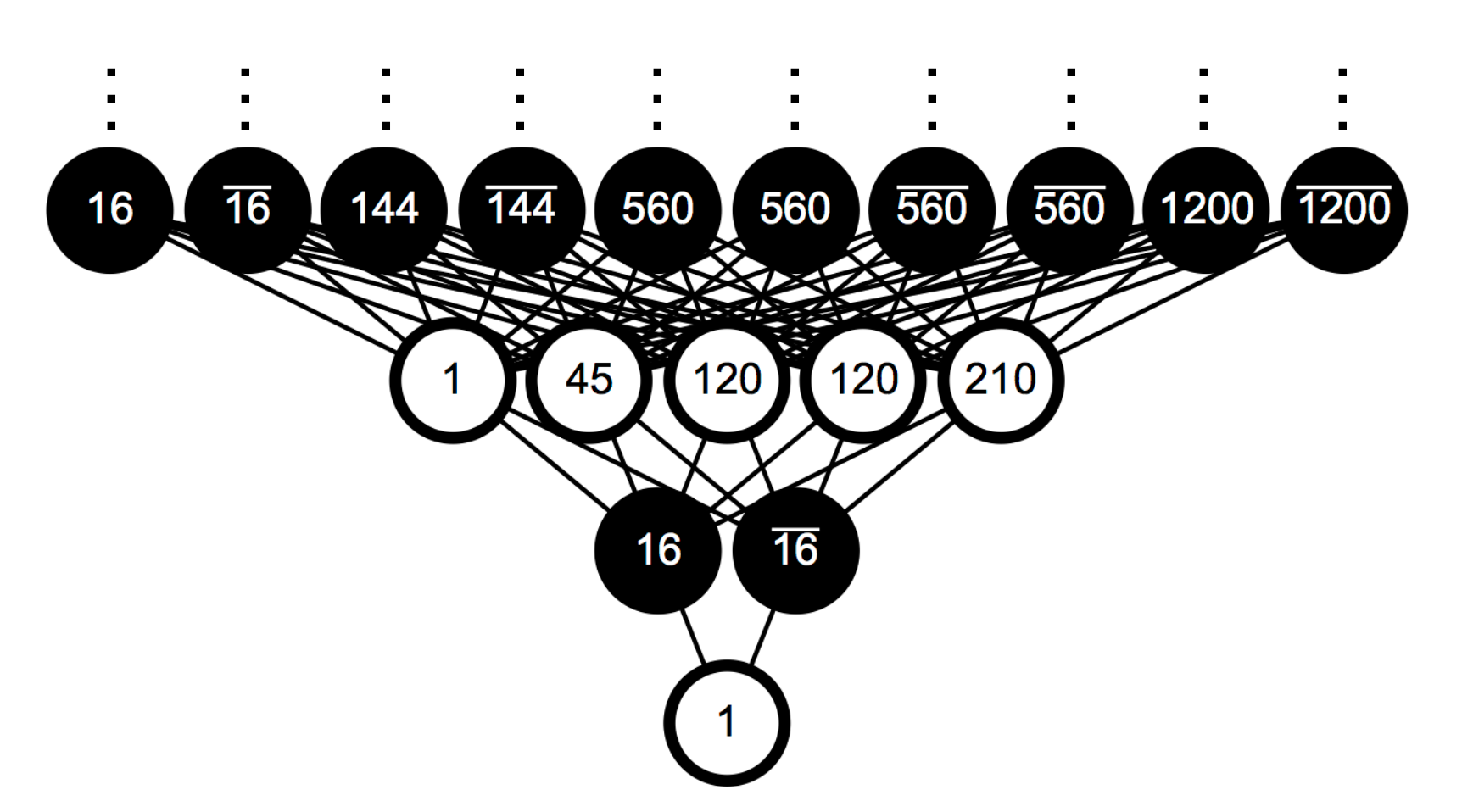
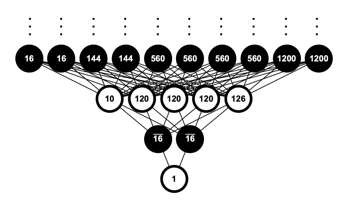
In a manner similar to how we drew the 4D, adinkra, we are now in position to explicitly demonstrate the 10D, adinkra by the same process. The adinkra with irrep dimensionality shown in each node is drawn in Figure 4.2, while the one with the corresponding Dynkin labels appears in Figure 4.2.
Indicated In Nodes
Indicated In Nodes
With this result, we have achieved two advances we believe to be significant.
(1.)
The graphs shown in Figure 4.2 and Figure 4.2 mark the first appearance
of ten dimensional adinkras in the literature.
(2.)
The graphs shown in Figure 4.2 and Figure 4.2 mark an independent con-
firmation of the component-level Lorentz representation
content of a 10D,
= 1 scalar superfield given by Bergshoeff and de Roo
[?].
Considering the case of 4D, = 1 supersymmetry, the graphs shown in Figure 4.2 and Figure 4.2 for the 10D, = 1 scalar superfield should be considered as the equivalents to the graph shown in Figure 3.1 for the 4D, = 1 scalar superfield. The obvious difference in “heights” was to be expected. However, a surprising feature is the maximum width of the 10D, = 1 scalar superfield adinkra is exactly the same as that of the 4D, = 1 scalar superfield, namely only three bosonic nodes. Another surprising feature of the 10D, = 1 scalar superfield is its economy. It only contains 15 independent bosonic field representations and 12 independent fermionic field representations.
A great and obvious challenge here is to discover the analog of the rules that govern the splitting that was described as to how 4D, = 1 chiral (irreducible) and 4D, = 1 vector (irreducible) adinkras can be obtained from a 4D, = 1 real scalar (reducible) adinkra.
4.4 The 10D, Adinkra & Nordström SG Components
In our previous work of [?], we found that the construction of 10D, supergravitation at the level of superfields and in terms of linearized supergeometry is very direct and without obstructions. It involved the introduction of a 10D, scalar superfield that appears in linearized frame operators in the forms
| (4.26) | ||||
| (4.27) |
Taking the 0 limit to the second of these equations implies that
| (4.28) |
where is a notation used to indicate the taking of the limit. The left hand side of this equation can be defined as
| (4.29) |
with describing the 10D graviton (expressed as a frame field) and describing the 10D gravitino. Combining the last two equations yields
| (4.30) |
In Nordström theory, only the non-conformal spin- part of graviton described by a scalar component field and the non-conformal spin- part of the gravitino
| (4.31) |
which is described by a component field show up. Both of these are appropriate for a Nordström-type theory.
Two of the results in the work of [?] take the respective forms
| (4.32) |
and
| (4.33) |
where . In the 0 limit, the first two terms of each of these equations involve the spacetime derivative of the scalar graviton in the theory. The final two terms in each of these equations involve the quantity corresponding to the Level-2 component field node shown in either of the adinkras shown in Figure 4.2 or Figure 4.2. It is the lowest dimensional auxiliary field of Nordström SG.
Application of a spinorial derivative to (i.e. ) yields the Level-3 fermionic component field node. Application of two spinorial derivatives to (i.e. ) yields the Level-4 and bosonic component field nodes. Application of three spinorial derivatives to (i.e. ) yields the Level-5 and fermionic component field nodes. Application of four spinorial derivatives to (i.e. ) yields the Level-6 and bosonic component field nodes. Application of five spinorial derivatives to (i.e. ) yields the Level-7 and fermionic component field nodes. Application of six spinorial derivatives to (i.e. ) yields the Level-8 , , and bosonic component field nodes.
From the form of the adinkras, we know that application of more than six fermionic derivatives to (or eight to ) only leads to the dual representations occurring. So for example seven fermionic derivatives applied to (or nine to ) must lead to the dual representations of those that occurred with the application of five fermionic derivatives (or seven to ). Thus, all the component fields of 10D, = 1 Nordström SG are obtained from (4.30) as well as applying all possible spinorial derivatives to the superspace covariant supergravity field strength followed by taking the 0 limit.
Thus, the knowledge of the 10D, = 1 scalar superfield adinkras provides an avenue to the complete component field description of the corresponding reducible Nordström supergravity theory derived from superspace geometry [?]. In particular, the knowledge that we know explicitly what representations can appear above the determines (up to some constants) the form of the solution of the superspace Bianchi Identities for the Nordström theory. When this is explicitly carried out, it opens the pathway to begin an exploration of dynamics in this context. However, this route to dynamics is similar in spirit to that of 10D, = 2B SG [?,?,?] where there is no action, but the equations for the dynamical fields in the supermultiplet are derived from analysis of the superspace Bianchi Identities alone. There is no a priori action required.
This is work for the future.
5 10D Breitenlohner Approach
In this chapter, we will apply the Breitenlohner approach to construct candidates for the 10D Type I superconformal multiplet. The principle of this approach is to attach bosonic and fermionic indices on the 10D scalar superfield, and search for the traceless graviton and the traceless gravitino.
Recall that the first off-shell description of 4D, = 1 supergravity was actually carried out by Breitenlohner [?], who took an approach equivalent to starting with the component fields of the Wess-Zumino gauge 4D, = 1 vector supermultiplet together with their familiar SUSY transformation laws
|
|
(5.1) |
followed by choosing as the gauge group the spacetime translations, SUSY generators, and the spin angular momentum generators as well as allowing additional internal symmetries. For the spacetime translation, this requires a series of replacements of the fields according to
|
|
(5.2) |
(in the notation in [?], is ). Because the vector supermultiplet is off-shell (up to WZ gauge transformations), the resulting supergravity theory is off-shell and includes a redundant set of auxiliary component fields, i. e. this is not an irreducible description of supergravity. But as seen from (5.2), the supergravity fields are all present, and together with the remaining component fields a complete superspace geometry can be constructed.
The key of this process is that if you look at Equation (3.3), there is a irrep (which is a vector gauge field) in level-2. When you consider the expansion of the superfield with one vector index which is also called the prepotential, you will find
| (5.3) |
where is the traceless graviton, as the degree of freedom is .
In 10D, theory, we want to search for the traceless graviton and the traceless gravitino . Let us first figure out which to which irreducible representations they correspond. The graviton has two symmetric vector indices, which corresponds to , and can be decomposed into the traceless part and the trace,
| (5.4) |
where both and are SO(1,9) irreps, while is not. In the following, we will denote the traceless graviton irrep to be , where the green color is added just to highlight this irrep. To determine the irreducible representations corresponding to the gravitino , first note that it has one vector index which corresponds to and one upper spinor index which corresponds to . We can then decompose the gravitino into its traceless part and its -trace part by the tensor product of these two irreps,
| (5.5) |
where the non-conformal spin- -trace part is defined in Equation (4.31). The traceless part of the gravitino is conformal, and this is what we should search for in the superconformal prepotential multiplet.
Now, if we hope to follow the exact same method in Equation (5.3), we would immediately confront the problem of the lacking of in the expansion in Equation (4.4). Therefore, we cannot introduce the 10D vector superfield as the prepotential and construct the off-shell conformal supergravity supermultiplet in the 10D, case right away. Instead, we attach other combinations of bosonic and fermionic indices onto the scalar superfields and search for traceless gravitons and gravitinos directly.
Given the Lorentz component content of a scalar superfield, how do we know the components of the superfields with various bosonic (or fermionic) indices? Let’s write out the scalar superfield expansion in Equation (4.1) again,
| (5.6) |
Attaching indices onto the scalar superfield would mean
| (5.7) |
where [indices] could be any combination of bosonic and/or fermionic indices, and it would correspond to a (sum of) bosonic or fermionic irreducible representation(s) in SO(1,9). If we let the level- monomial decompositions of 10D, scalar superfield be for , the level- component field content would be . For simplicity, consider only the [indices] that corresponds to one and only one irreducible representation {irrep}. Then the level- component field content of would be {irrep}. We denote the component content of the entire superfield by the expression {irrep}, which we will use throughout the following sections.
In the following two sections, we will study the expansions of some bosonic and fermionic superfields respectively to see whether we can identify possible off-shell supergravity supermultiplet(s). This is the meaning of the term “scanning.” Once more we emphasize that our arguments are totally group theoretical and therefore do not rely on dynamical assumptions.
5.1 Bosonic Superfields
We will start by attaching bosonic indices on the 10D, = 1 scalar superfield, which is equivalent to tensoring the corresponding bosonic irreps to the component decomposition of the scalar superfield. Here we explicitly study these bosonic irreps: , , , , , , , , , and . The summary of their expansions is listed in Table 6. The third column shows which tensor product contributes to , and the decomposition results show that each one only provides one .
| Dynkin Label | Irrep | Is there ? |
| no | ||
| no | ||
| level-0: | ||
| level-4: | ||
| level-8: | ||
| level-2: | ||
| level-6: | ||
| no | ||
| no | ||
| level-4: | ||
| level-8: | ||
| no | ||
| level-2: | ||
| level-6: | ||
| level-8: | ||
| level-4: | ||
| level-8: |
Of course, the result for is not surprising and can be removed as a candidate for a conformal 10D, = 1 supergravity prepotential. All of the other entries in the table do provide candidate prepotentials. It is noticeable that several of these candidates ( , , and ) allow conformal graviton embeddings at the eighth level. If Wess-Zumino gauges exist to eliminate lower order bosons, these imply “short” supergravity multiplets.
Now, one can look into one of those bosonic superfields with traceless gravitons in detail as an example. The irreps shown here are component fields. The reader can find other bosonic superfields with traceless gravitons in Appendix C.
| (5.8) |
where Level-9 to Level-16 are conjugate of Level-7 to Level-0 respectively.
The superfield can be interpreted as , a three form (three totally antisymmetric Lorentz indices). It provides four possibilities for the embedding of traceless gravitons (at level-2, level-6, level-10, and level-14). Note that if one finds a in level-, one finds a at level-. This holds for all bosonic superfields listed in Table 6. We can see this relation between graviton and gravitino clearly by considering the SUSY transformation law of the graviton in 10D theory. We know the undotted D-operator acting on the graviton represented by gives a term proportional to the undotted gravitino in the on-shell case (in the off-shell case, there are several auxiliary fields showing up in the r.h.s. besides the undotted gravitino)
| (5.9) |
Note that the undotted spinor index on the gravitino is a superscript. According to our convention, corresponds to the irrep . Recall that acting the D-operator once will add one to the level. Thus, Equation (5.9) is exactly the mathematical expression of the statement that if you find a in level-, you will find a in level-.
Based on Equation (5.8), we can see four possible embeddings for the graviton, ten possible embeddings for the gravitino, along with a number of auxiliary fields. The superfield is also the simplest nontrivial bosonic superfield that contains traceless gravitons and gravitinos and can be used as the starting point to construct supergravity. In fact, as long ago as 1982, Howe, Nicolai, and Van Proeyen [?] had suggested this particular superfield might be an appropriate point from which to construct a prepotential for 10D, = 1 supergravity.
However, our more general study provides the basis for constructing possible viable theories. It also provides new insights into the origin of constraints in these systems.
Notice that has one and only one conformal graviton candidate at level-8. In recalling the structure of 4D, = 1 supergravity theory, there it was seen the supergravity prepotential contained only a single field of the appropriate Lorentz representation to be identified with a conformal graviton and that was precisely at the “middle level” of the -expansion. This immediately implies a question. One can ask the question of how unique is this occurence? To answer this, we created a search routine to explore other possible “external tensor indices” in addition to the above bosonic irreps. Table 7 shows all the irreps up to dimension 73710, that when tensored on a scalar superfield, gives a bosonic superfield that have this property. These irreps all have congruency class (00).
| Dynkin Label | Irrep |
|---|---|
From this investigation it is obvious that the frequency of occurence of possessing a single graviton within a supermultiplet that occurs at the middle level in the -expansion of superfield is not a rare event.
We know the representation possesses a graviton condidate at Level-0 while the representation possesses a graviton candidate at Level-8. The interesting thing about the representation is that it may regarded as part of the linearization of the full 10D, frame field . This means one can write an equation of the form
| (5.10) |
which has the effect of implying that the graviton condidate at Level-0 in and the graviton candidate at Level-8 in the representation are one and the same field. In this equation, the quantity are a set of quantities chosen so that the equation is consistent with SO(1,9) Lorentz symmetry.
Without this equation, is unconstrained. However, when this equation is imposed, it causes constraints that involve the operator to be imposed on . This is the origin of SG constraints for the perspective of adinkras. Of course, the example we chose is only one possibility. One could make other choices in place of the representation. This would require using other orders of the operator and an appropriate replacement of the -tensor. This is determined by where the candidate representation occurs in final superfield in the equation. Finally, though we only considered bosonic superfields above, with further appropriate modifications the can be replaced by fermionic superfields.
5.2 Fermionic Superfields
Now we investigate fermionic superfields by attaching spinor indices onto the scalar superfield. Here are the spinorial irreps we will explicitly explore: , , , , , , , , , and . Before we present our results, some words of motivation will likely serve the cause of explaining the purpose of doing so.
Ever since the work of [?], it has been known that the prepotential superfield description of 4D, = 2 supergravity is described by a fundamental dynamical entity that is fermionic. As a 4D, = 2 supersymmetrical theory can be descended from a 6D minimally supersymmetrical one, this clearly points out the possibility that higher dimensional theories can possess fermionic supergravity prepotentials.
There is a second reason why the study of fermionic superfields is suggested. Some time ago [?], efforts were undetaken to investigate the structure of 1-form 10D, = 1 gauge theories as theories involving superspace superconnections over fiber bundles. This study reached a conclusion that all off-shell theories of this type must include a bosonic component field . This observation was later confirmed by a number of subsequent studies [?,?,?,?]. This leads to a powerful restriction if the scanning process is applied to the 1-form 10D, = 1 gauge theories. At the same level in the expansion in Grassmann coordinates, both the and the SO(1,9) representations must be present. In addition, there must also occur the at one level higher in the expansion to accommodate an accompanying gaugino. In a subsequent section we will discuss the relevance of the features uncovered to the case of the 1-form 10D, = 1 gauge theory. Furthermore, in order to reach the maximal level of simplication in our presentation, we will only consider the abelian case for the 1-form 10D, = 1 gauge theory.
We will begin by only considering the feature revealed by our tensoring that are relevant to the case of 10D, = 1 supergravity theory. The summary of the expansions for the fermionic cases is listed in Table 8. The third column shows which tensor product contributes and the decomposition results show that each one only contributes one .
| Dynkin Label | Irrep | Is there ? |
| no | ||
| no | ||
| level-1: | ||
| level-5: | ||
| level-3: | ||
| level-7: | ||
| level-5: | ||
| level-3: | ||
| level-7: | ||
| no | ||
| no | ||
| level-1: | ||
| level-5: | ||
| level-3: | ||
| level-7: |
Now, one can look at one of those fermionic superfields with traceless gravitons in some detail as an example. The cases of other fermionic superfields with embeddings for traceless gravitons are given in Appendix D. Generally for , here we only list level-0 to level-8 results, and its level-9 to level-16 are conjugate of level-7 to level-0 of .
can be interpreted as , a fermionic superfield with two antisymmetric bosonic indices and one spinor index satisfying
| (5.11) |
It provides three possible embeddings for traceless gravitons in total (in level-5, level-9, and level-13). Note that if you find a in level-, you can find a in level-. This holds for all fermionic superfields listed in Table 8, which is consistent with Equation (5.9).
There exists a work [?] in the literature from 1987, where the proposal for the use of a fermionic 10D, = 1 supergravity prepotential was first given. However, the proposed prepotential was of the form which is equivalent to .
Based on Equation (5.12), we see three possible embeddings for gravitons, fifteen possible embeddings for gravitinos, and auxiliary fields. The superfield is also the simplest nontrivial fermionic superfield that contains traceless gravitons and gravitinos and can be used to construct supergravity.
| (5.12) |
5.3 10D, Yang-Mills Supermultiplet
The work previously described in this chapter on fermionic superfields also opens the doorway for using the techniques developed so far in this paper to the issue of scanning the component level description of a superspace connection used to define a 1-form U(1) superspace covariant derivatives
| (5.13) |
where denotes the U(1) generator and is a coupling constant. The commutators of two covariant derivatives take the forms [?]
| (5.14) | |||
| (5.15) | |||
| (5.16) | |||
| (5.17) |
The equations below are consistent with the solutions of Bianchi identities [?]
| (5.18) |
and
| (5.19) |
The results immediately above are the most important. They show that if the component field variable is set to zero on the RHS of these equations, then the spinorial photino field and the bosonic Maxwell field must both satisfy their equations of motion. Stated another way, for these two component fields to be off-shell, it requires the presence of the condition 0.
In the work of [?], the structures of the spinorial gauge connection superfield and its gauge parameter up to level-4 in are given by
| (5.20) | ||||
| (5.21) | ||||
respectively. The irreducible component fields in Figure 4.2 and Figure 4.2 are contained in in the following way. The component fields in at levels 0, 1, 2, and 3 in the -expansion correspond to the nodes at the same height assignments in the adinkra. The component field at level-4 in the -expansion of is to be expanded solely over the the irreducible representations shown at the fourth level of the adinkra. The component content of the connection superfield is encoded by tensoring the components of the scalar superfield with a lower spinor index, i.e. .
| (5.22) |
By comparing this with Equation (5.20), we read that in level-0 corresponds to ; level-1 , and correspond to , and ; level-2 corresponds to which is exactly the decomposition at level-2 of (5.22), where is the level-2 monomial of the scalar superfield. One point to note is that is but not . This is because it is contracted with which a self-dual 5-form by Equation (4.13). The conditions for embedding the component fields into requires at some level- (here ) there must occur and the while at the level- there must occur a , as we noted earlier.
Now, if we want to put the gauge fields to the middle level and apply Wess-Zumino gauge, we look for superfields that have gauge fields and at level-8, and the gaugino at the next level, i.e. level-9. And we want the triplet (, , and ) to show up at level-8 and 9 only. Table 9 shows all the irreps (up to dimension 73710) that when tensored into the scalar superfield, would give us the superfields with that property. It also shows the numbers of gauge 1-form(s), gauge 5-form(s) and gaugino(s) in level-8 and 9 that appear in each superfield listed. We denote them by . All these irreps have conjugacy class (02).
| Dynkin Label | Irrep | |
|---|---|---|
| (1,1,1) | ||
| (1,2,2) | ||
| (1,1,1) | ||
| (1,2,1) | ||
| (1,2,1) | ||
| (1,2,1) | ||
| (1,2,1) | ||
| (1,3,1) |
All the remarks that were made at the end of the discussion regarding the possibility of the conformal supergravity theory apply with minor modifications here.
6 10D, A Scalar Superfield Decomposition and Superconformal Multiplet
6.1 Methodology for 10D, A Scalar Superfield Construction
One can introduce two sets of 10D spinor coordinates denoted by and so that a 10D, superfield can be expressed in the form . It is possible to organize the expansion so that it takes the form
| (6.1) |
and the point is that each of the expansion coefficients , , is a 10D, superfield. More explicitly, from Equation (4.1) one can write
| (6.2) |
Attaching totally antisymmetric dotted ’s to an undotted monomial corresponds to tensoring the representation on it, i.e. tensoring the conjugate of the th level of the monomial of the 10D, scalar superfield on it. Therefore, if we denote level- monomial of 10D, scalar superfield as , we can obtain the 10D, A scalar superfield monomial decomposition by
| (6.3) |
and level-17 to 32 are the conjugates of level-15 to 0 respectively. From Equation (6.3), it’s clear that each level is self-conjugate and therefore level-17 to 32 are the same as level-15 to 0. Moreover, the decompositions of component fields are the same as that of the monomials.
6.2 10D, A Scalar Superfield Decomposition Results and Superconformal Multiplet
Based on Equations (4.4) and (6.3), one can directly obtain the scalar superfield decomposition in 10D, A. The results from level-0 to level-16 are listed below. We use green color to highlight the irrep which corresponds to the traceless graviton in 10D. Unlike in 10D, theory, one can find possible embeddings for gravitons and gravitinos in the expansion of the scalar 10D, A superfield. As discussed in chapter 3, we can translate irreps into component fields and see 72 graviton embeddings, 280 gravitino embeddings, and associated hosts of auxiliary fields. The scalar superfield is the simplest superfield that contains traceless gravitons and gravitinos and can be used to construct supergravity.
Note that if you find a in level-, you can find and in level-. This is also consistent with SUSY transformation laws of the graviton in 10D, A theory. Acting the undotted D-operator on the graviton gives a term proportional to the undotted gravitino in the on-shell case (in the off-shell case, there are several auxiliary fields showing up in the r.h.s. besides the undotted gravitino)
| (6.4) |
Note that the gravitino here has an undotted superscript spinor index and hence corresponds to irrep in our convention. Meanwhile the dotted D-operator acting on the graviton satisfies
| (6.5) |
which gives a term proportional to the dotted gravitino in the on-shell case. The superscript dotted spinor index on the gravitino indicates that it corresponds to irrep in our convention.
-
•
Level-0:
-
•
Level-1:
-
•
Level-2:
-
•
Level-3:
-
•
Level-4:
-
•
Level-5:
-
•
Level-6:
-
•
Level-7:
-
•
Level-8:
-
•
Level-9:
-
•
Level-10:
-
•
Level-11:
-
•
Level-12:
-
•
Level-13:
-
•
Level-14:
-
•
Level-15:
-
•
Level-16:
6.3 Adinkra Diagram for 10D, A Superfield
In this section, we present the ten dimensional A adinkra diagram up to the cubic level. Based on the results listed in Section 6.2, we can draw the complete adinkra diagram in principle: use open nodes to denote bosonic component fields and put their corresponding irreps in the center. For fermionic component fields, use closed nodes. The number of level represents the height assignment. Black edges connect nodes in the adjacent levels, meaning SUSY transformations. Due to the limited space of the paper, we only draw the adinkra up to the cubic level.
7 10D, B Scalar Superfield Decomposition and Superconformal Multiplet
7.1 Methodology for 10D, B Scalar Superfield Construction
The Type IIB theory means , i.e. we have two sets of spinor coordinates denoted by and . Following the same logic as in Type IIA, one can organize the B scalar superfield as
| (7.1) |
where the expansion coefficients , , are 10D, superfields. Attaching another copy of totally antisymmetric undotted ’s to an undotted monomial corresponds to tensoring the representation on it, i.e. the th level of the monomial of the 10D, superfield itself, without any conjugate. Therefore, the B scalar superfield monomial decomposition can be summarized as
| (7.2) |
and level-17 to 32 are the conjugates of level-15 to 0 respectively. The irreps corresponding to the component fields are the conjugates of the monomials at each level.
7.2 10D, B Scalar Superfield Decomposition Results and Superconformal Multiplet
Based on Equations (4.4) and (7.2), we can directly obtain the scalar superfield decomposition in 10D, B. The results for monomials from level-0 to level-16 are listed below. Same as in the Type IIA case, we can find graviton embeddings and gravitino embeddings in the expansion of the scalar superfield. We use green color to highlight the irrep which corresponds to the traceless graviton in 10D as well. We can translate irreps into component fields and see 72 graviton embeddings, 280 gravitino embeddings, and accompanying auxiliary fields. The scalar superfield is the simplest superfield that contains traceless graviton and gravitino embeddings that can be used as a starting point to construct supergravity. The numbers of gravitons and gravitinos are the same as those in Type IIA case.
Note that if one find a in level-, one can find in level-, which can be interpreted by SUSY transformation laws of the graviton in 10D, B theory. Since in Type IIB theory we have two copies of rather than and , we have D-operators where . Acting the D-operators on the graviton gives a term proportional to the gravitino in the on-shell case (in the off-shell case, there are several auxiliary fields showing up in the r.h.s. besides the undotted gravitino)
| (7.3) |
Note that the spinor indices on the gravitinos are superscript. It suggests that the gravitinos correspond to irrep in our convention for both and . In the context of monomials, the conjugate of is still , and the conjugate of is .
-
•
Level-0:
-
•
Level-1:
-
•
Level-2:
-
•
Level-3:
-
•
Level-4:
-
•
Level-5:
-
•
Level-6:
-
•
Level-7:
-
•
Level-8:
-
•
Level-9:
-
•
Level-10:
-
•
Level-11:
-
•
Level-12:
-
•
Level-13:
-
•
Level-14:
-
•
Level-15:
-
•
Level-16:
7.3 Adinkra Diagram for 10D, B Superfield
Here we draw the ten dimensional B adinkra diagram up to the cubic level.
8 Conclusion
This work gives a new group-theoretic free-of-dynamics method for the complete decompositions of scalar superfields to irreducible component field representations of the 10D Lorentz group, and a proposal for identifying the corresponding superconformal multiplets by applying the Breitenlohner approach in , A, and B superspaces. The new results here provide a foundation for future extensions. Our efforts also mark a new beginning for the search for irreducible off-shell formulations of the 10D Yang-Mills supermultiplet derived from superfields.
We believe it is important to comment on the graphs shown in Figure 1.1 in comparisons to those shown in Figure 4.2, Figure 4.2, Figure 6.1, and Figure 7.1. While the latter two of these are incomplete101010The only reason for their incompleteness is convenience of presentation., they share an attribute with those in Figure 4.2 and Figure 4.2. The graphs in Figure 1.1 were constructed by starting from an off-shell component formulation. In contrast, the graphs in Figure 4.2, Figure 4.2, Figure 6.1, and Figure 7.1 were constructed without any information from a component formulation. The presentations of the latter four graphs provide demonstrations that with this work a new level of completeness has been achieved about the structure of superfields in high dimensions.
There is a certain tension in the path we are pursuing with the use of adinkras and superfields in comparison with the well established results in the literature. Many years ago, Nahm [?] pointed out the absence of a superconformal current above six dimensions. This most certainly suggests an obstruction may exist.
On the other hand, in works going back decades [?,?,?,?,?], there have been increasing explorations of the concepts of conformal symmetry within the context of 10D superspaces. Our scans suggest the possibilities of a number of superfields for embedding the component-level conformal gravitons into 10D superfields. This supports the idea of the eventual success of these efforts. Though we do not understand how this tension will be resolved… if it can… we would point the reader to what may prove to be a similar situation.
In the works of [?,?], the Witt algebra (i.e. the “centerless Virasoro algebra”) was investigated. It was found that the form of the Witt algebra undergoes a radical change dependent on the number of supercharges under investigation. When the number of supercharges is four or less, the form of the Witt algebra is simple and uniform. However, when the number of supercharges exceeds four, the form of the Witt algebra changes dramatically with the appearance of new generators that are not present for the cases when the number of supercharges is less than four. It seems likely to us this phenomenon may provide a route by which these embeddings that are obvious from the supergeometrical side could lead to conformal supergravity theories in higher dimensions.
In a future work, we will also dive far more deeply into the relations between analytical expressions of the irreducible monomials, Young Tableaux, and Dynkin labels. Along a different direction of future activities lies the extension of our results to the case of 11D, = 1 supergravity. The results in this work regarding the case of the 10D, = 2A supergravity theory already contain a lot of information about the eleven dimensional theory as it is equivalent upon toroidal compactification to the 10D, = 2A supergravity theory. In principle, it is straightforward to construct the component level contents from our approach that uses branching rules. However, in practice this is considerably more computationally challenging than the equivalent work in the 10D, = 2A supergravity theory. Currently the work on this is underway.
We end by concisely summarizing a surprising and heretofore unknown result discovered in this work and cast it into the form of a conjecture.
Consider a Lorentz superspace of signature SO(1, D - 1) and let denote the dimension of the smallest spinor representation consistent with this signature. Furthermore, let , and denote a set of non-negative integers. Finally, let , and respectively denote the dimensionality of some bosonic and fermionic representations of the SO(1, D - 1) Lorentz algebra. For a scalar superfield in this superspace, the number of bosonic degrees of freedom at the -th level of the corresponding adinkra is given by for even values of and the number of fermionic degrees of freedom at the -th level of the corresponding adinkra is given by for odd values of .
Conjecture:
Let denote a scalar superfield in
a Lorentz superspace of signature SO(1, D - 1),
then at each even level of the superfield the equation
| (8.1) |
and at each odd level of the superfield the equation
| (8.2) |
are both determined by the
branching rules of the totally antisymmetric representa-
tions of series of the Cartan classification of compact Lie algebras
under the
projection to its SO(1, D - 1) subalgebra.
“Our knowledge can only be finite, while our ignorance
must necessarily be infinite.”
- Karl Popper
Acknowledgements
This research of S. J. G., Y. Hu, and S.-N. Mak is supported in part by the
endowment of the Ford Foundation Professorship of Physics at Brown University.
S. J. G. makes an additional acknowledgment to the National Science
Foundation grant PHY-1620074 and all the authors gratefully acknowledge
the support of the Brown Theoretical Physics Center. Additionally, we acknowledge
the referee whose critique spurred expanded historical and content additions
to the final version of this work.
Appendix A Chiral and Vector Supermultiplets from the 4D, Unconstrained Scalar
Superfield
In this appendix, we present an expanded discussion of the mathematical structures that support the validity of the “splitting” of the adinikras presented in Figure 3.3. The vector supermultiplet shown in the figure is well familiar, but this is not so for the chiral supermultiplet shown. We will begin with the vector supermultiplet. The notational conventions used in the following discussion are those of Superspace [?].
The vector supermultiplet contains a 1-form gauge potential that is part of a super 1-form with different sectors given by
| (A.1) |
The vector supermultiplet field strength superfield is determined in terms of an unconstrained real scalar superfield by
| (A.2) |
The definition of is invariant under gauge transformations with a chiral parameter that takes the form
| (A.3) |
The components of the prepotential superfield can be defined by the projection method
| (A.4) |
All the components of can be gauged away by nonderivative gauge transformations except for , , , and , where the vector and spinor are the physical components and is auxiliary component. We find the action to be
| (A.5) |
However, a superfield with the same structure as can also be used to describe an entirely different supermultiplet. To distinguish this second supermultiplet from the first, we will use the symbol to denote its prepotential. This second supermultiplet contains a 3-form gauge potential that is part of a super 3-form with different sectors given by
| (A.6) |
This super 3-form theory has been discussed previously in the works of [?,?] and more recently in [?] in terms of component fields.
The chiral supermultiplet that is contained in a real unconstrained scalar superfield has a gauge invariant superfield field strength of the form
| (A.7) |
where the prepotential has gauge transformations
| (A.8) |
The physical component fields of this gauge 3-form multiplet are
| (A.9) |
The quantity is the field strength of the component gauge 3-form , so that the field strength is invariant. Interpreted the other way, the chiral supermultiplet is that with component content , and the supermultiplet corresponding to the bottom right diagram of Figure 3.3 is one of the Hodge-dual variants111111There are three of them. Two of them can correspond to Figure 3.3 with one of the auxiliary fields replaced by its Hodge-dual - see equations (3.6) and (3.7) in [?]. The third one is obtained by replacing both of the auxiliary fields to their Hodge-duals, as shown in (3.8) in the reference. of the chiral supermultiplet with component content . This is done by taking one of the auxiliary fields to its Hodge-dual gauge 3-form as shown in the last line of (A.9).
The action for this supermultiplet is given by
| (A.10) |
and when this is evaluated at the level of component fields, this action contains the d’Alembertian for the complex component scalar field , the Dirac operator for the component spinor , the square of - the kinetic term for the component 3-form and the square of - real spin-0 auxiliary field.
Appendix B SO(10) Irreducible Representations
Here we list the SO(10) irreducible representations by Dynkin labels and dimensions [?].
| Dynkin label | Dimension |
|---|---|
| (00000) | |
| (10000) | |
| (00001) | |
| (00010) | |
| (01000) | |
| (20000) | |
| (00100) | |
| (00020) | |
| (00002) | |
| (10010) | |
| (10001) | |
| (00011) | |
| (30000) | |
| (11000) | |
| (01001) | |
| (01010) | |
| (40000) | |
| (00030) | |
| (00003) | |
| (20001) | |
| (20010) | |
| (02000) | |
| (10100) | |
| (10020) | |
| (10002) | |
| (00110) | |
| (00101) | |
| (21000) | |
| (00012) | |
| (00021) | |
| (10011) | |
| (50000) | |
| (30010) | |
| (30001) | |
| (00040) | |
| (00004) |
| Dynkin label | Dimension |
|---|---|
| (01100) | |
| (11010) | |
| (11001) | |
| (01020) | |
| (01002) | |
| (00200) | |
| (60000) | |
| (20100) | |
| (12000) | |
| (31000) | |
| (20020) | |
| (20002) | |
| (10003) | |
| (10030) | |
| (01011) | |
| (00120) | |
| (00102) | |
| (00031) | |
| (00013) | |
| (03000) | |
| (40001) | |
| (40010) | |
| (02001) | |
| (02010) | |
| (20011) | |
| (10101) | |
| (10110) | |
| (00022) | |
| (70000) | |
| (00005) | |
| (00050) | |
| (00111) |
Appendix C Bosonic Superfield Decompositions
In this appendix, we list a few bosonic superfields that contain the traceless graviton and the traceless gravitino and . Here every irrep corresponds to a component field.
| (C.1) |
| (C.2) |
| (C.3) |
| (C.4) |
| (C.5) |
Appendix D Fermionic Superfield Decompositions
In this appendix, we list a few fermionic superfields that contain the traceless graviton and the traceless gravitino and . Here every irrep corresponds to a component field.
| (D.1) |
| (D.2) |
| (D.3) |
| (D.4) |
| (D.5) |
References
- [1] S.J. Gates, Jr., Y. Hu, H. Jiang, and S.-N. Hazel Mak, “A codex on linearized Nordstršm supergravity in eleven and ten dimensional superspaces,” JHEP 1907 (2019) 063, DOI: 10.1007/JHEP07(2019)063, e-Print: arXiv:1812.05097 [hep-th]
- [2] E. Bergshoeff, and M. de Roo, “The Supercurrent in Ten Dimensions,” Phys. Lett. 112B (1982) 53, DOI: 10.1016/0370-2693(82)90904-2.
- [3] P. Breitenlohner, “A Geometric Interpretation of Local Supersymmetry,” Phys. Lett. 67B (1977) 49, DOI: 10.1016/0370-2693(77)90802-4.
- [4] M.F. Sohnius, “Supersymmetry and Central Charges,” Nucl. Phys. B138, 109 (1978) doi:10.1016/0550-3213(78)90159-1.
- [5] M.F. Sohnius, K.S. Stelle, and P.C. West, “Dimensional Reduction By Legendre Transformation Generates Off-Shell Yang-Mills Theories,” Nucl. Phys. B173, 127 (1980) DOI:10.1016/0550-3213(80)90447-2.
- [6] J.D. Taylor, “Off-Shell Central Charges and Linearized N = 8 Supergravity,” Phys. Lett. 107B, 217 (1981) DOI:10.1016/00370-2693(81)90815-7.
- [7] R. D’Auria, P. Fré, and A.J. da Silva, “Geometric Structure of N=1,D=10 and N=4,D=4 Super yang-mills Theory,” Nucl. Phys. B196, 205 (1982) DOI: 10.1016/0550-3213(82)90036-0.
- [8] H. Nicolai, and A. Van Proeyen, “Off-shell Representations With Central Charges For Ten-dimensional Super Yang-mills Theory,” Nucl. Phys. B203, 510 (1982) DOI: 10.1016/0550-3213(82)90328-5.
- [9] M. Faux, S. J. Gates Jr., “Adinkras: A Graphical Technology for Supersymmetric Representation Theory,” Phys. Rev. D71 (2005) 065002, e-Print: arXiv:1812.05097 [hep-th] [hep-th/0408004].
- [10] C. F. Doran, K. Iga, and G. Landweber, “An application of Cubical Cohomology to Adinkras and Supersymmetry Representations,” July 2012, 1207.6806, e-Print: arXiv:1207.6806 [hep-th], (unpublished).
- [11] Yan X. Zhang, “Adinkras for Mathematicians,” Transactions of the American Mathematical Society, Vol. 366, No. 6, June 2014, Pages 3325-355, DOI: 10.1090/S0002-9947-2014-06031-5.
- [12] C. F. Doran, M. G. Faux, S. J. Gates, Jr., T. Hübsch, K. M. Iga, and G. D. Landweber, “On Graph-Theoretic Identifications of Adinkras, Supersymmetry Representations and Superfield,” Int. J. Mod. Phys. A22 (2007) 869-930, DOI: 10.1142/S0217751X07035112, e-Print: math-ph/0512016.
- [13] S. J. Gates, Jr. and S. Vashakidze, “On , Supersymmetry, Superspace Geometry and Superstring Effects,” Nucl. Phys. B 291, 172 (1987). doi:10.1016/0550-3213(87)90470-6.
- [14] C. F. Doran, M. G. Faux, S. J. Gates, Jr., T. Hübsch, K. M. Iga, G. D. Landweber, and R. L. Miller, “Topology Types of Adinkras and the Corresponding Representations of N-Extended Supersymmetry,” UMDEPP-08-010, SUNY-O-667, e-Print: arXiv:0806.0050 [hep-th].
-
[15]
C. F. Doran, M. G. Faux, S. J. Gates, Jr., T. Hübsch, K. M. Iga, and
G. D. Landweber, “Re-
lating Doubly-Even Error-Correcting Codes, Graphs, and Irreducible Representations of N-
Extended Supersymmetry,” UMDEPP-07-012 SUNY-O-663, e-Print: arXiv:0806.0051 [hep-th]. - [16] C. F. Doran, M. G. Faux, S. J. Gates, Jr., T. Hübsch, K. M. Iga, G. D. Landweber, and R. L. Miller, “Codes and Supersymmetry in One Dimension,” Adv. Theor. Math. Phys. 15 (2011) 6, 1909-1970; e-Print: arXiv:1108.4124.
- [17] C. Doran, K. Iga, J. Kostiuk, G. Landweber, and S. Mendez-Diez, “Geometrization of N-extended 1-dimensional supersymmetry algebras, I,” Adv. Theor. Math. Phys. 19 (2015) 1043-1113, DOI: 10.4310/ATMP.2015.v19.n5.a4. e-Print: arXiv:1311.3736 [hep-th].
- [18] C. Doran, K. Iga, J. Kostiuk, G. Landweber, and S. Mendez-Diez, “Geometrization of N-Extended 1-Dimensional Supersymmetry Algebras II,” Adv.Theor.Math.Phys. 22 (2018) 565-613, DOI: 10.4310/ATMP.2018.v22.n3.a2, e-Print: arXiv:1610.09983 [hep-th].
- [19] S. J. Gates. Jr., T. Hübsch, and K. Stiffler, “On Clifford-algebraic ‘Holoraumy’, dimensional extension and SUSY holography,” Int. J. Mod. Phys. A30 (2015) no.09, 1550042, DOI: 10.1142/S0217751X15500426, e-Print: arXiv:1409.4445 [hep-th].
- [20] M. Calkins, D. E. A. Gates, S. J. Gates. Jr., and K. Stiffler, “Adinkras, 0-branes, Holoraumy and the SUSY QFT/QM Correspondence,” Int. J. Mod. Phys.A30 (2015) no.11, 1550050, DOI: 10.1142/S0217751X15500505, e-Print: arXiv:1501.00101 [hep-th].
- [21] S.J. Gates, Jr. and , S.-N. Hazel Mak, “Examples of 4D, N = 2 holoraumy,” Int.J.Mod.Phys. A34 (2019) no.17, 1950081 e-Print: arXiv:1808.07946 [hep-th] DOI: 10.1142/S0217751X19500817.
- [22] S. J. Gates, Jr., Y. Hu, and K. Stiffler, “Adinkra Height Yielding Matrix Numbers: Eigenvalue Equivalence Classes for Minimal Four-Color Adinkras,” Int.J.Mod.Phys. A34 (2019) no.18, 1950085 e-Print: arXiv:1904.01738 [hep-th], DOI: 10.1142/S0217751X19500854.
- [23] C. F. Doran, M. G. Faux, S. J. Gates, Jr., T. Hubsch, K. M. Iga, G. D. Landweber, “On the Matter of N=2 Matter,” Phys.Lett.659B: 441-446,2008, DOI: 10.1016/j.physletb.2007.11.001.
- [24] M. Faux, “The Conformal Hyperplet,” Int.J.Mod.Phys. A32 (2017) no.14, 1750079, DOI: 10.1142/S0217751X17500798, e-Print: arXiv:1610.07822 [hep-th].
- [25] P,S. Howe, K.S. Stelle, P.K. Townsend, “Superactions,” Nucl. Phys. B191 (1981) 445-464 DOI: 10.1016/0550-3213(81)90308-4.
- [26] P,S. Howe, K.S. Stelle, P.K. Townsend, “Supercurrents,” Nucl. Phys. B192 (1981) 332-352 DOI: 10.1016/0550-3213(81)90429-6.
- [27] P,S. Howe, K.S. Stelle, P.K. Townsend, “The Relaxed Hypermultiplet: An Unconstrained N=2 Superfield Theory,” Nucl. Phys. B214 (1983) 519-531, DOI: 10.1016/0550-3213(83)90249-3.
- [28] N. Yamatsu, “Finite-dimensional Lie algebras and their representations for unified model building,” arXiv:1511.08771 (2015) (unpublished).
- [29] R. Slansky, “Group theory for unified model building,” Phys. Reports. 79 (1981) 1-128, DOI: 10.1016/0370-1573(81)90092-2.
- [30] D.E, Littlewood, “The Theory of group characters,” 2nd Ed. (Oxford U.P., Oxford, 1950).
- [31] F.D. Murnaghan, “The theory of group representations,” (The Johns Hopkins Press, Baltimore, 1938).
- [32] R. Feger and T. W. Kephart, “LieART—A Mathematica application for Lie algebras and representation theory,” Comput. Phys. Commun. 192, 166 (2015) doi:10.1016/j.cpc.2014.12.023 [arXiv:1206.6379 [math-ph]].
- [33] C. F. Doran, M. G. Faux, S. J. Gates, Jr., T. Hubsch, K. M. Iga and G. D. Landweber, “Adinkras and the Dynamics of Superspace Prepotentials,” hep-th/0605269. (unpublished).
- [34] M. G. Faux, K. M. Iga, and G. D. Landweber, “Dimensional Enhancement via Supersymmetry,” Adv. Math. Phys. 2011 (2011) 259089, DOI: 10.1155/2011/259089, e-Print: arXiv:0907.3605 [hep-th].
- [35] M. G. Faux, and G. D. Landweber, “Spin Holography via Dimensional Enhancement,” Phys. Lett. B681 (2009) 161-165, DOI: 10.1016/j.physletb.2009.10.014, e-Print: arXiv:0907.4543 [hep-th].
- [36] S. J. Gates, Jr,, “Spacetime Spin and Chirality Operators for Minimal 4D, N = 1 Supermultiplets From BC4 Adinkra-Tessellation of Riemann Surfaces,” Jan 27, 2017. 12 pp. (unpublished), UNIV.-OF-MARYLAND-PREPRINT-PP-017-019, BROWN-UNIVERSITY-PREPRINT-HET-1709 e-Print: arXiv:1701.08102 [hep-th],
- [37] T. Curtright, “Fundamental Supermultiplet In Twelve-dimensions,” Front. in Phys. 6 (2018) 137, DOI: 10.3389/fphy.2018.00137.
- [38] P. S. Howe, and P. C. West, “The Complete N = 2, D = 10 Supergravity,” Nucl. Phys. B238 (1984) 181, DOI: 10.1016/0550-3213(84)90472-3.
- [39] M. T. Grisaru, P. Howe, L. Mezincescu, B. Nilsson, and P. Townsend, “N = 2 Superstrings in a Supergravity Background,” Phys. Lett. 162B (1985) 116, DOI: 10.1016/0370-2693(85)91071-8.
- [40] S. Bellucci. S.J. Gates, Jr., B. Radak, and Sh. Vashakidze. “Improved Supergeometries for Type-II Green-Schwarz Nonlinear Model,” Mod.Phys.Lett. A4 (1989) 1985-1998, DOI: 10.1142/S0217732389002240
- [41] P,S. Howe, H. Nicolai, and A. Van Proeyen, “Auxiliary Fields and a Superspace Lagrangian for Linearized Ten-dimensional Supergravity,” Phys.Lett.B112: 446-450,1982, DOI: 10.1016/0370-2693(82)90845-0.
- [42] S.J. Gates, Jr., and W. Siegel “Linearized N=2 Superfield Supergravity,” Nucl. Phys. B195 (1982) 39-60, DOI: 10.1016/0550-3213(82)90047-5.
- [43] E. Bergshoeff, M. Rakowski, an E. Sezgin, “Higher Derivative Super Yang-mills Theories,” Phys.Lett. 185B (1987) 371-376, DOI: 10.1016/0370-2693(87)91017-3.
- [44] S.F. Kerstan, “Supersymmetric Born-Infeld from the D9-brane,” Class.Quant.Grav. 19 (2002) 4525-4536, DOI: 10.1088/0264-9381/19/17/304, e-Print: hep-th/0204225.
- [45] N. Berkovits, and P.S. Howe, “The Cohomology of superspace, pure spinors and invariant integrals,” JHEP 0806 (2008) 046, DOI: 10.1088/1126-6708/2008/06/046, e-Print: arXiv:0803.3024.
- [46] P.S. Howe, U. Lindstrom, and L. Wulff, “D=10 supersymmetric Yang-Mills theory at ,” JHEP 1007 (2010) 028, DOI: 10.1007/JHEP07(2010)028, e-Print: arXiv:1004.3466.
- [47] W. Nahm, “Supersymmetries and their representations,” Nucl. Phys. B135 (1978) 149. DOI: 10.1016/0550-3213(78)90218-3.
- [48] E. Bergshoeff, M. de Roo, B. de Wit, P. van Nieuwenhuizen, “Ten-Dimensional Maxwell-Einstein Supergravity, Its Currents, and the Issue of Its Auxiliary Fields,” Nucl.Phys. B195 (1982) 97-136, DOI: 10.1016/0550-3213(82)90050-5.
- [49] E. Bergshoeff, M. de Roo, and B. de Wit, “Conformal Supergravity in Ten-dimensions,” Nucl.Phys. B217 (1983) 489, DOI: 10.1016/0550-3213(83)90159-1.
- [50] S.J. Gates, Jr., and H. Nishino, “Realization of space-time conformal symmetry in D = 10, N=1 superspace,” Phys.Lett. 266B (1991) 14-20 DOI: 10.1016/0370-2693(91)90737-B.
- [51] M. de Roo, “The R2-action in d=10 conformal supergravity,” Nucl. Phys. B372, (1992) 243-269, DOI: 10.1016/0550-3213(92)90319-7.
- [52] S.J, Gates, Jr., and L. Rana “Superspace geometrical representations of extended super Virasoro algebras,” Phys.Lett. B438 (1998) 80-88, DOI: 10.1016/S0370-2693(98)00937-X e-Print: hep-th/9806038.
- [53] S. J. Gates, Jr., W. D. Linch, III, J. Philips, and V.G.J. Rodgers “Short Distance Expansion from the Dual Representation of Infinite Dimensional Lie Algebras,” Commun.Math.Phys. 246 (2004) 333, DOI: 10.1007/s00220-004-1048-0 e-Print: hep-th/0211021.
- [54] S. J. Gates, Jr., M. T. Grisaru, M. Roček, and W. Siegel, “Superspace Or One Thousand and One Lessons in Supersymmetry,” Front. Phys. 58 (1983) 1-548, e-Print: hep-th/0108200.
- [55] S. J. Gates, Jr. “Super P Form Gauge Superfields,” Nucl. Phys. B184 (1981) 381-390 DOI: 10.1016/0550-3213(81)90225-X.
- [56] W. Caldwell, A. N. Diaz, I. Friend, S. J. Gates, Jr., S. Harmalkar, T. Lambert-Brown, D. Lay, K. Martirosova , V. A. Meszaros, M. Omokanwaye, S. Rudman, D. Shin, and A. Vershov, “On the four-dimensional holoraumy of the 4D, N = 1 complex linear supermultiplet,” Int. J. Mod. Phys. A33 (2018) no.12, 1850072, DOI: 10.1142/S0217751X18500720. e-Print: arXiv:1702.05453 [hep-th].