Abstract

The integrated nested Laplace approximation (INLA) for Bayesian inference is an efficient approach to estimate the posterior marginal distributions of the parameters and latent effects of Bayesian hierarchical models that can be expressed as latent Gaussian Markov random fields (GMRF). The representation as a GMRF allows the associated software R-INLA to estimate the posterior marginals in a fraction of the time as typical Markov chain Monte Carlo algorithms. INLA can be extended by means of Bayesian model averaging (BMA) to increase the number of models that it can fit to conditional latent GMRF. In this paper we review the use of BMA with INLA and propose a new example on spatial econometrics models.

xx 1 5 Received: date; Accepted: date; Published: date Bayesian model averaging with the integrated nested Laplace approximation Virgilio Gómez-Rubio, ^1,†,‡*, Roger S. Bivand ^2,‡ and Håvard Rue^3,‡ Virgilio Gómez-Rubio, Roger S. Bivand and Håvard Rue Correspondence: Virgilio.Gomez@uclm.es; Tel.: +34-967-59-92-00, ext. 8291 Current address: Department of Mathematics, School of Industrial Engineering, Universidad de Castilla-La mancha, Avda. España s/n, 02071 Albacete (Spain) These authors contributed equally to this work.

1 Introduction

Bayesian model averaging (BMA, see, for example, Hoeting et al., 1999) is a way to combine different Bayesian hierarchical models that can be used to estimate highly parameterized models. By computing an average model, the uncertainty about the model choice is taken into account when estimating the uncertainty of the model parameters.

As BMA often requires fitting a large number of models, this can be time consuming when the time required to fit each of the models is large. The integrated nested Laplace approximation (INLA, Rue et al., 2009) offers an alternative to computationally intensive Markov chain Monte Carlo (MCMC, Gilks et al., 1996) methods. INLA focuses on obtaining an approximation of the posterior marginal distributions of the models parameters of latent GMRF models (Rue and Held, 2005). Hence, BMA with INLA is based on combining the resulting marginals from all the models averaged.

Bivand et al. (2014, 2015) use this approach to fit some spatial econometrics models by fitting conditional models on some of the hyperparameters of the original models. The resulting models are then combined using BMA to obtain estimates of the marginals of the hyperparameters of the original model. Gómez-Rubio and Rue (2018) have embedded INLA within MCMC so that the joint posterior distribution of a subset of the model parameters is estimated using the Metropolis-Hastings algorithm (Metropolis et al., 1953; Hastings, 1970). This requires fitting a model with INLA (conditional on some parameters) at each step, so that the resulting models can also be combined to obtain the posterior marginals of the remainder of the model parameters.

BMA with INLA relies on a weighted sum of the conditional marginals obtained from a family of conditional models on some hyperparameters. Weights are computed by using Bayes’ rule and they depend on the marginal likelihood of the conditional model and the prior distribution of the conditioning hyperparameters. This new approach is described in detail in Section 4. We will illustrate how this works by developing an example on spatial econometrics models described in Section 2.

This paper is organized as follows. Spatial econometrics models are summarized in Section 2. Next, an introduction to INLA is given in Section 3. This is followed by a description of Bayesian model averaging (with INLA) in Section 4. An example is developed in Section 5. Finally, Section 6 gives a summary of the paper and includes a discussion on the main results.

2 Spatial econometrics models

Spatial econometrics models (LeSage and Pace, 2009) are often employed to account for spatial autocorrelation in the data. Usually, these models include one or more spatial autoregressive terms. Manski (1993) propose a model that includes an autoregressive term on the response and another one in the error term:

$$y=\rho Wy+X\beta+WX\gamma+u$$

Here, $y$ is the response, $X$ a matrix of covariates with coefficients $\beta$, $W$ an adjacency matrix and $WX$ are lagged covariates with coefficients $\gamma$. Finally, $u$ is an error term. This error term is often modeled to include spatial autocorrelation:

$$u=\lambda Wu+e$$

Here, $e$ is a vector of Gaussian observations with zero mean and precision $\tau$.

The previous model can be rewritten as

$$y=(I-\rho W)^{-1}(\beta X)+u^{{}^{\prime}}$$

with $u^{{}^{\prime}}$ an error term with a Gaussian distribution with zero mean and precision matrix

$$\tau(I-\rho W^{\top})(I-\lambda W^{\top})(I-\lambda W)(I-\rho W)$$

Note that here the same adjacency matrix $W$ has been used for the two autocorrelated terms, but different adjacency matrices could be used. The range of $\rho$ and $\lambda$ is determined by the eigenvalues of $W$. When $W$ is taken to be row-standardized, the range is the interval $(1/m,1))$, where $m$ is the minimum eigenvalue of $W$ (see, for example, Haining, 2003). In this case, the lagged covariates $WX$ represent the average value at the neighbors, which is useful when interpreting the results.

In a Bayesian context, a prior needs to be set on every model parameter. For the spatial autocorrelation parameter a uniform in the interval $(-1,1)$ will be used. For the coefficients of the covariates, a Normal with zero mean and precision 1000 is used, and for precision $\tau$ Gamma with parameters $0.01$ and $0.01$.

This model is often referred to as spatial autoregressive combined (SAC) model. Other important models in spatial econometrics appear when some of the terms in the SAC model are dropped. See, for example, Gómez-Rubio et al. (2017) and how these models are fit with INLA.

In spatial econometrics models it is of interest how changes in the value of the covariates affect the response in neighboring regions. These spill-over effects or impacts (LeSage and Pace, 2009) are caused by the term $(I-\rho W)^{-1}$ that multiplies the covariates and they are defined as

$$\frac{\partial y_{i}}{\partial x_{jk}},\ i,j=1,\ldots,n;\ k=1,\ldots,p$$

where $n$ is the number of observations and $p$ the number of covariates and $x_{jk}$ is the value of covariate $k$ in region $j$.

Hence, for each covariate $k$ there will be an associated matrix of impacts. The diagonal values are known as direct impacts as they measure the effect of changing a covariate on the same areas. The off-diagonal values are known as indirect impacts as they measure the change of the response at neighboring areas when covariate $k$ changes. Finally, total impacts are the sum of direct and indirect impacts.

Gómez-Rubio et al. (2017) describe how the impacts are for different spatial econometrics models. For the SAC model, the impacts matrix for covariate $k$ are

$$S_{r}(W)=(I-\rho W)^{-1}I\beta_{r}$$

In practice, average impacts are reported as a summary of the direct, indirect and total impacts (for details see, for example, LeSage and Pace, 2009; Gómez-Rubio et al., 2017). In particular, the average direct impact is the trace of $S_{r}(W)$ divided by $n$, the average indirect impact is defined as the sum of the off-diagonal elements divided by $n$ and the average total impact is the sum of all elements of $S_{r}(W)$ divided by $n$. Average total impact is also the sum of the average direct and average indirect impacts.

For the SAC model, the average total impact is $\beta_{r}/(1-\rho)$ and the average direct impact is $n^{-1}tr((I-\rho W)^{-1})\beta_{r}$. The average indirect impact can be computed as the difference between the average total and average direct impacts, $[1/(1-\rho)-n^{-1}tr((I-\rho W)^{-1})]\beta_{r}$, or by computing the sum of the off-diagonal elements of $S_{r}(W)$ divided by $n$.

Note that computing the impacts depends on parameters $\rho$ and $\beta_{r}$. For this reason, the joint posterior distribution of both parameters would be required. A explained below, this is not a problem because it can be rewritten as $\pi(\beta_{r},\rho\mid\mathbf{y})=\pi(\beta_{r}\mid\mathbf{y},\rho)\pi(\rho\mid\mathbf{y})$.

3 The integrated nested Laplace approximation

Markov chain Monte Carlo algorithms (see, for example, Brooks et al., 2011) are typically used to estimate the joint posterior distribution of the ensemble of parameters and latent effects of a hierarchical Bayesian model. However, these algorithms are often slow when dealing with high parameterized models.

Recently Rue et al. (2009), have proposed a computationally efficient numerical to estimate the posterior marginals of the hyperparameters and latent effects. This method is called integrated nested Laplace approximation (INLA) because it is based on repeatedly using the Laplace approximation to estimate the posterior marginals. In addition, INLA focuses on models that can be expressed as a latent Gaussian Markov random files (GMRF, Rue and Held, 2005).

In this context, the model is expressed as follows. For each observation $y_{i}$ in the ensemble of observations $y$, its likelihood is defined as

$$y_{i}|\bm{\theta},\mathbf{x}\sim f(y_{i}|\bm{\theta},\mathbf{x}),\ i=1,\ldots,n$$

For each observation $y_{i}$, its mean $\mu_{i}$ will be conveniently linked to the linear predictor $\eta_{i}$ using the appropriate function (which will depend on the likelihood used). The linear predictor will include different additive effects such as fixed effects and random effects.

Next, the vector of latent effects $\mathbf{x}$ is defined as a GMRF with zero mean and precision matrix $\Sigma$ (which may depend on the vector of hyperparameters $\bm{\theta}$):

$$\mathbf{x}\sim GMRF(0,\Sigma(\bm{\theta}))$$

Finally, the hyperparameters are assigned a prior distribution. This is often done assuming prior independence. Without loss of generality, this can be represented as

$$\bm{\theta}\sim\pi(\bm{\theta})$$

Note that $\pi(\bm{\theta})$ is a multivariate distribution but that in many cases it can be expressed as the product of several univariate (or small dimension) prior distributions.

Hence, if $\bm{\theta}$ represents the vector of $h$ hyperparameters and $\bm{x}$ the vector of $l$ latent effects, INLA provides the posterior marginals

$$\{\pi(\theta_{i}|\mathcal{D})\}_{i=1}^{h}$$

and

$$\{\pi(x_{i}|\mathcal{D})\}_{i=1}^{l}$$

Note that $\mathcal{D}$ represents the observed data, and it includes response $y$, covariates $\mathbf{X}$ and any other known quantities required for model fitting.

In addition to the marginals, INLA can be used to estimate other quantities of interest. See, for example, Rue et al. (2017) for a recent review.

INLA can provide accurate approximations to the marginal likelihood of a model, which are computed as

$$\tilde{\pi}(\mathcal{D})=\int\frac{\pi(\bm{\theta},\mathbf{x},\mathcal{D})}{\tilde{\pi}_{\mathrm{G}}(\mathbf{x}|\bm{\theta},\mathcal{D})}\bigg{\lvert}_{\mathbf{x}=\mathbf{x^{*}}(\bm{\theta})}d\bm{\theta}.$$

Here, $\tilde{\pi}_{\mathrm{G}}(\mathbf{x}|\bm{\theta},\mathcal{D})$ is a Gaussian approximation to the distribution of $\mathbf{x}\mid\bm{\theta},\mathcal{D}$, and $\mathbf{x^{*}}(\bm{\theta})$ is the posterior mode of $\mathbf{x}$ for a given value of $\bm{\theta}$. This approximation seems to be accurate in a wide range of examples (Hubin and Storvik, 2016; Gómez-Rubio and Rue, 2018).

As described in Section 4, the marginal likelihood plays a crucial role in BMA as it determines the weights, together with the prior distribution of some of the hyperparameters in the model.

As stated above, INLA approximates the posterior marginals of the parameters of latent GMRF models. Hence, an immediate question is whether INLA will work for different models. Gómez-Rubio and Rue (2018) introduce the idea of using INLA to fit conditional latent GMRF models by conditioning on some of the hyperparameters. In this context, the vector of hyperparameters $\bm{\theta}$ is split into $\bm{\theta}_{c}$ and $\bm{\theta}_{-c}$, so that models are fit with INLA conditional on $\bm{\theta}_{c}$ and the posterior marginals of the elements of $\bm{\theta}_{-c}$ and latent effects $\mathbf{x}$ are obtained, i.e., $\pi(\theta_{-c,i}\mid\mathcal{D},\bm{\theta}_{c})$ and $\pi(x_{j}\mid\mathcal{D},\bm{\theta}_{c})$, respectively. Here, $\theta_{-c,i}$ represents any element in $\bm{\theta}_{-c}$ and $x_{j}$ any element in $\mathbf{x}$.

In practice, this involves setting hyperparameters $\bm{\theta}_{c}$ to some value, so that the model becomes a latent GMRF that INLA can tackle. Gómez-Rubio and Rue (2018) provide some ideas on how these can be chosen. Gómez-Rubio and Palmí-Perales (2019) propose setting these values to maximum likelihood estimates (for example) and other options and provide examples that show that this may still provide good approximations to the posterior marginal distributions of the remainder of the parameters in the model.

4 Bayesian model averaging with INLA

As stated above, fitting conditional models by setting some hyperparameters ($\bm{\theta}_{c}$) to fixed values can be a way to use INLA to fit wider classes of models. However, this ignores the uncertainty about these hyperparameters $\bm{\theta}_{c}$ and makes inference about them impossible. However, BMA may help to fit the complete model, even if it cannot be fit with INLA initially.

First of all, it is worth noting that the posterior marginals (of the hyperparameters $\bm{\theta}_{-c}$ and latent effects $\mathbf{x}$) can be written as

$$\pi(\cdot\mid\mathcal{D})=\int\pi(\cdot,\bm{\theta}_{c}\mid\mathcal{D})d\bm{\theta}_{c}=\int\pi(\cdot\mid\mathcal{D},\bm{\theta}_{c})\pi(\bm{\theta}_{c}\mid\mathcal{D})d\bm{\theta}_{c}$$

The first term in the integrand, $\int\pi(\cdot\mid\mathcal{D},\bm{\theta}_{c})$, is the conditional posterior marginals given $\bm{\theta}_{c}$, while the second term is the joint posterior distribution of $\bm{\theta}_{c}$ and it can be expressed as

$$\pi(\bm{\theta}_{c}\mid\mathcal{D})\propto\pi(\mathcal{D}\mid\bm{\theta}_{c})\pi(\bm{\theta}_{c})$$

The first term is the conditional (on $\bm{\theta}_{c}$) marginal likelihood which can be approximated with INLA. The second term is the prior for $\bm{\theta}_{c}$, which is known. Hence, the posterior distribution of $\bm{\theta}_{c}$ could be computed by re-scaling the previous expression.

Bivand et al. (2014) show that when $\bm{\theta}_{c}$ is unidimensional, numerical integration can be used to estimate the posterior marginal. This is done by using a regular grid of $K$ values $\{\theta^{(i)_{c}}\}_{i=1}^{K}$ of fixed step $h$.

Hence, the posterior marginals of the remainder of hyperparameters and latent effects can be estimated as

$$\pi(\cdot\mid\mathcal{D})\simeq\sum_{i=1}^{K}\pi(\cdot\mid\mathcal{D},\theta_{c}^{(i)})\ w_{i}$$

with weights $w_{i}$ defined as

$$w_{i}=\frac{\pi(\mathcal{D}\mid\theta^{(i)}_{c})\pi(\theta_{c}^{(i)})}{\sum_{i=1}^{K}\pi(\mathcal{D}\mid\theta^{(i)}_{c})\pi(\theta_{c}^{(i)})}$$

Note how the posterior marginal $\pi(\cdot\mid\mathcal{D})$ is expressed as a BMA using the conditional posterior marginals of all the fit models.

Inference on $\bm{\theta}_{c}$ is based on the values $\{\theta^{(i)_{c}}\}_{i=1}^{K}$ and weights $\{w_{i}\}^{K}$. For example, the posterior mean of the element $j$-th in $\bm{\theta}_{c}$ could be computed as $\sum_{i=1}^{K}\theta_{c,j}w_{i}$. Other posterior quantities could be computed similarly. Note that this also allows for multivariate posterior inference on the elements of $\bm{\theta}_{c}$.

This can be easily extended to higher dimensions by considering that the proposed values of $\bm{\theta}_{c}$ fill the space in subsets of equal volume. In practice, it is not necessary to consider the complete space (as it is not feasible) but the region of posterior high probability of $\bm{\theta}_{c}$. This may be obtained by, for example, maximizing $\pi(\mathcal{D}\mid\bm{\theta}_{c})\pi(\bm{\theta}_{c})$, which can be easily computed with INLA or by using a maximum likelihood estimate if available (as discussed, for example, in Gómez-Rubio and Palmí-Perales, 2019).

5 Example: turnover in Italy

In order to provide an example of the methodology presented in previous sections we will take the turnover dataset described in Ward and Gleditsch (2008), which is available from website http://ksgleditsch.com/srm_book.html. This dataset records the turnover in the 2001 Italian elections, as well as GDP per capita (GDPCAP) in 1997 (in million Lire). The data comprises 477 areas, which represent collegi or single member districts (SDM). Adjacency has been defined so that regions whose centroids are 50 km or less away are neighbors to ensure that all regions have neighbors, contiguous regions are neighbors, and Elba is joined to the closest mainland region. In order to assess the impact of the GDP per capita in the estimation of the spatial autocorrelation parameters, two models with and without the covariate will be fit.

Figure 1 shows the spatial patterns of these two variables. As it can be seen, there is a clear south-north pattern for both variables. Hence, we are interested in fitting spatial econometrics models on turnover in 2011 using GDP per capita in 1997 as predictor so that residual spatial autocorrelation is captured by the two autoregressive terms in the model.

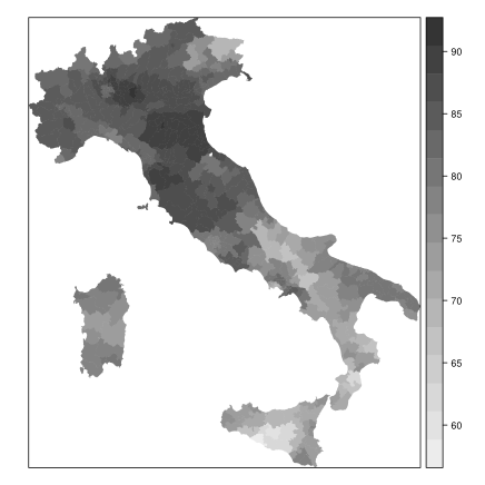
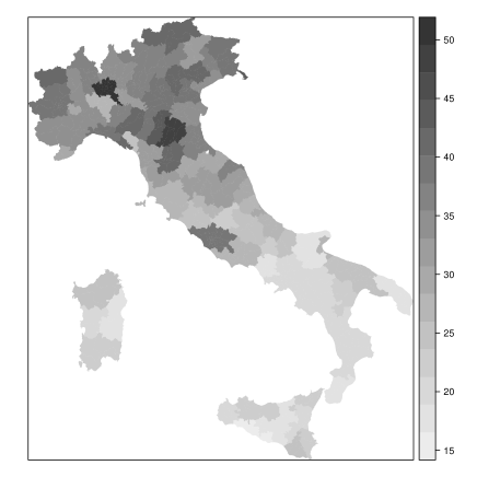
Figure 1: Spatial distribution of turnover in 2011 (left) and GDP per capita in 1997 (right) in Italy at the collegi level.

The SAC model will be fit with INLA by conditioning on the values of the two spatial autocorrelation parameters. As described in Section 2, after conditioning the resulting model is a typical mixed-effects model with a particular matrix of covariates and a known structure for the precision matrix of the random effects. Hence, we are considering $\bm{\theta}_{c}=(\rho,\lambda)$.

Both autocorrelation parameters are given values in the range (-1, 1). Note that, because the same adjacency matrix is used, the actual domain for both parameters is $(1/\lambda_{min},1)$, with $\lambda_{min}$ the minimum eigenvalue of the adjacency matrix $W$. In this case, $\lambda_{min}=-0.82$ so taking the range $(-1,1)$ will be enough.

Maximum likelihood estimates of the models will be obtained with package spdep (Bivand et al., 2013), and MCMC estimates will be obtained with package spatialreg (Bivand and Piras, 2015; Bivand et al., 2013). For MCMC, we used 10000 burn-in iterations, plus another 90000 iterations for inference, of which only one in ten was kept to reduce autocorrelation. To speed up convergence, the initial values of $\rho$ and $\lambda$ were set to their maximum likelihood estimates. BMA with INLA estimates will be obtained as explained next.

A regular grid about the posterior mode of $(\rho,\lambda)$ will be created for each model using the maximum likelihood estimates. The grid is defined in an internal scale to have unbounded variables using the transformation $\gamma_{1}=\log(\frac{1+\rho}{1-\rho})$ and $\gamma_{2}=\log(\frac{1+\lambda}{1-\lambda})$. The variance of $\gamma_{1}$ and $\gamma_{2}$ can be derived using Delta method (see Appendix A for details), and it can be computed using the ML standard error estimate of $\rho$ and $\lambda$. In particular, each interval is centered at the transformed ML estimate and a semi-amplitude of three standard errors of the variables in the internal scale. See Table 1 for the actual values of the ML estimates. Furthermore, a grid of $160\times 40$ points was used to represent the search space and fit the conditional models with R-INLA for the model without the covariate and a grid of $40\times 20$ for the model with GDPCAP. A different grid was used because the model without the covariate required a thinner grid.

Table 1 provides a summary of the estimates of the model parameters using different inference methods. First of all, maximum likelihood (ML) estimates (computed with function sacsarlm in the spdep package). Next, $\rho$ and $\lambda$ have been fixed at their ML estimates and the model has been fit with INLA. Next, the posterior marginals of the model parameters using BMA with INLA and MCMC are shown. In general, point estimates obtained with the different methods provide very similar values. MCMC and maximum likelihood also provide very similar estimates of the uncertainty of the point estimates (when available for maximum likelihood). BMA with INLA seems to provide very similar results to MCMC for both models.

		Max. lik.		INLA - Max. lik.		BMA		MCMC
Model	Parameter	Mean	St. error	Mean	St. dev.	Mean	St. dev.	Mean	St. error
No covariates	$\beta_{0}$	5.86	1.54	5.88	0.10	6.39	1.59	6.56	1.95
	$\rho$	0.93	0.02	0.93	–	0.92	0.02	0.92	0.02
	$\lambda$	0.09	0.10	0.09	–	0.12	0.10	0.12	0.10
	$\tau^{-1}$	3.66	–	3.68	0.24	3.71	0.25	3.75	0.28
Covariates	$\beta_{0}$	8.33	2.46	8.33	0.37	9.46	2.44	9.53	3.04
	$\beta_{1}$	0.05	0.02	0.05	0.01	0.05	0.02	0.05	0.02
	$\rho$	0.88	0.03	0.88	–	0.86	0.03	0.86	0.04
	$\lambda$	0.17	0.11	0.17	–	0.22	0.11	0.21	0.12
	$\tau^{-1}$	3.77	–	3.79	0.24	3.82	0.26	3.89	0.31

Table 1: Summary statistics of the model parameters.

Note the positive coefficient of GDP per capita, which means a positive association with turnout. Furthermore, the spatial autocorrelation $\rho$ has a higher value than $\lambda$, which indicates higher autocorrelation on the response than on the error term.

Figure 2 shows the values of the marginal log-likelihoods of all the conditional models fit as well as the weights used in BMA. Note the wide variability of the marginal log-likelihoods that makes the weights to be very small. Weights are almost zero for most models but a few of them. Note that this is good because it indicates that the search space for $\rho$ and $\lambda$ is adequate and that the region of high posterior density has been explored.

Figure 2: Weights and marginal likelihoods for the model with no covariates (top row) and with covariates (bottom row).

Figure 3 shows the posterior marginals of the spatial autocorrelation parameters using kernel smoothing (Venables and Ripley, 2002). For the BMA output weighted kernel smoothing, has been used. In general, there is good agreement between BMA with INLA and MCMC. The ML estimates are also very close to the posterior modes.

Figure 3: Posterior marginals of the spatial autocorrelation parameters for the model with no covariates (top row) and with covariates (bottom row).

Similarly, Figure 4 shows the joint posterior distribution of the autocorrelation parameters obtained using two-dimensional kernel smoothing. For the BMA output this has been obtained using two-dimensional weighted kernel smoothing with function kde2d.weighted in package ggtern (Hamilton and Ferry, 2018). The ML estimate has also been added (as a black dot). As with the posterior marginals, the joint distribution is close between MCMC and BMA with INLA. The posterior mode is also close to the ML estimate. The plots show a negative correlation between the spatial autocorrelation parameters, which may indicate that they struggle to explain spatial correlation in the data (see also Gómez-Rubio and Palmí-Perales, 2019). Furthermore, BMA with INLA is a valid approach to make joint posterior inference on a subset of hyperparameters in the model.

Figure 4: Joint posterior distribution of the spatial autocorrelation parameters for the model with no covariates (top row) and with covariates (bottom row). The black dot represents the maximum likelihood estimate.

These results shows the validity of relying on BMA with INLA to fit highly parameterized models. This approach also accounts for the uncertainty of all model parameters and should be preferred to other inference methods based on plugging-in or fixing some of the models parameters. In our case, we have relied on BMA with INLA so that conditional sub-models are fit and then combined. This has two main benefits. First of all, allows for full inference on all model parameters and, secondly, uncertainty about all parameters is taken into account.

Figure 5 shows the posterior marginals of the coefficients and the variance of the models. In general, BMA with INLA and MCMC show very similar results for all parameters The posterior modes of MCMC and BMA with INLA are very close to the ML estimates. Marginals provided by INLA with ML estimates are very narrow for the fixed effects, which is probably due to ignoring the uncertainty about the spatial autocorrelation parameters.

Figure 5: Posterior marginal distributions of the coefficients and variances for the model with no covariates (top row) and with covariates (bottom row).

Computation of the impacts is important because they measure how changes in the values of the covariates reflect on changes of the response variable in the current area (direct impacts) and neighboring areas (indirect impacts). Note that impacts are only computed for the model with the covariate included. Table 2 shows the estimates of the different average impacts. In general, all estimation methods provide very similar values of the point estimates, and BMA with INLA and MCMC estimates are very close. Figure 6 displays the posterior marginal distributions of the average impacts. Again, these estimates are very similar among estimation methods.

	Max. lik.		INLA - Max. lik.		BMA		MCMC
Impact	Mean	St. dev.	Mean	St. dev.	Mean	St. dev.	Mean	St. dev.
Direct	0.07	–	0.07	0.02	0.07	0.02	0.07	0.02
Indirect	0.32	–	0.33	0.08	0.32	0.08	0.31	0.09
Total	0.39	–	0.40	0.09	0.39	0.09	0.38	0.10

Table 2: Average impacts estimated with the different methods.

Figure 6: Posterior marginals of the average direct (left), indirect (middle) and total (right) impacts of the GDP per capita.

6 Discussion

Bayesian model averaging with the integrated nested Laplace approximation has been illustrated to make inference about the parameters and latent effects of highly parameterized models. The appeal of this methodology is that it relaxes the constraints on the model that does not need to be latent GMRF anymore but conditional latent GMRF. This has been laid out with an example based on spatial econometrics models.

Cheaper alternatives to BMA include setting the values of a subset of the hyperparameters to their posterior modes or maximum likelihood estimates. This can still produce accurate estimates of the posterior marginals of the remainder of the parameters in the model (Gómez-Rubio and Palmí-Perales, 2019) but ignores the uncertainty about some parameters in the model as well as any posterior inference about them.

Although we have used numerical integration methods to estimate the joint posterior distribution of the conditioning hyperparameters, this is limited to low dimensions and it may not scale well. However, other approaches could be used such as MCMC algorithms (Gómez-Rubio and Rue, 2018).

Finally, BMA with INLA makes inference about a small subset of hyperparameters in the mode possible. This is an interesting feature as INLA focuses on marginal inference and joint posterior analysis require sampling from the internal representation of the latent field (Gómez-Rubio, 2019), which can be costly. We have also shown how this can be used to compute the posterior marginals distribution of derived quantities (i.e., the impacts) that depend on a small subset of hyperparameters. Our results with BMA with INLA are very close to those obtained with MCMC, which supports the use of BMA with INLA as a feasible alternative for multivariate posterior inference.

Appendix A Implementation details

A.1 Model fitting

Implementation of the SAC model with INLA is done in two steps. First, the model is fit given $\rho$ and $\lambda$. Given these values, the model is a linear mixed-effects model with design matrix of the fixed effects equal to

$$(I-\rho W)^{-1}X$$

and the vector of random effects has mean zero and precision matrix

$$\tau\Sigma,$$

where $\tau$ is a precision parameter to be estimated. Matrix $\Sigma$ is a precision matrix fully determined (given that $\rho$ and $\lambda$ are known) and it is

$$\Sigma=(I-\rho W^{\top})(I-\lambda W^{\top})(I-\lambda W)(I-\rho W).$$

This model can be fit with the R-INLA package using a Gaussian likelihood, and a design matrix for the fixed effects $(I-\rho W)^{-1}X$ and latent random effects with zero mean and precision matrix $\tau\Sigma$. In particular, the latent random effects can be defined using effect generic0. Furthermore, the precision of the Gaussian likelihood is set to $\exp(15)$ to remove the error term. Otherwise, the model would include another error term in the linear predictor in addition to fixed and random effects. Higher values of the precision led to unstable estimates of the model and the marginal likelihood.

The generic0 latent effects is a multivariate Gaussian distribution with zero mean and precision matrix $\tau\Sigma$. Because $\Sigma$ is known, its determinant is ignored by R-INLA when computing the log-likelihood. For this reason, we have added $+\frac{1}{2}\log(|\Sigma|)$ to the computation of the marginal likelihood reported by R-INLA, with $|\Sigma|$ the determinant of $\Sigma$.

Once the different models have been fit, weights $w_{i}$ are computed as in Section 4. Models are merged using function inla.merge, that takes the list of models fit and the vector of weights.

A.2 Grid definition

As stated in Section 5 the grid to explore the values of $(\rho,\lambda)$ is a regular grid defined in an internal scale to make the internal parameters unbounded. The estimate of the variance of the parameters in the internal scale can be obtained by using the Delta method. The transformation used is $\gamma_{1}=\log(\frac{1+\rho}{1-\rho})$ and $\gamma_{2}=\log(\frac{1+\lambda}{1-\lambda})$. If we consider $g(x)=\log(\frac{1+x}{1-x})$, then $\gamma_{1}=g(\rho)$ and $\gamma_{2}=g(\lambda)$. Hence, the inverse transformation can be considered if we take function $f(x)=2\frac{\exp(x)}{1+\exp(x)}-1$, and the original parameters are defined as $\rho=f(\gamma_{1})$ and $\lambda=f(\gamma_{2})$.

The Delta method states that if $\sigma^{2}$ is the variance of a variable $x$, then an estimate of the variance of $g(x)$ is $\sigma^{2}(g^{{}^{\prime}}(x))^{2}$, with $g^{{}^{\prime}}(x)$ the first derivative of $g(x)$. In our case, we have that

$$g^{{}^{\prime}}(x)=\frac{2}{(1+x)(1-x)}.$$

Using ML estimation, for both $\rho$ and $\lambda$ an estimate of the variance is provided by their respective squared standard errors. Hence, the estimate of the variance of $\gamma_{1}$ is

$$se_{\rho}^{2}(\frac{2}{(1+\rho)(1-\rho)})^{2}$$

Here, $se_{\rho}$ is the standard error of $\rho$ and $\rho$ represents the ML estimate. Similarly, an estimate of the variance of $\gamma_{2}$ is developed.

Note that because the regular grid is defined in the internal scale, the prior should be on $\gamma_{1}$ and $\gamma_{2}$. This can be derived (Chapter 5, Gómez-Rubio, 2019) by considering a correction due to the transformation. For example, the prior on $\rho$ is a uniform in the interval $(-1,1)$ which has a constant density in that interval. The prior on $\gamma_{1}$, $\pi(\gamma_{1})$, is $\pi(\rho)|\frac{\partial\rho}{\partial\gamma_{1}}|$, with

$$\frac{\partial\rho}{\partial\gamma_{1}}=\frac{\partial(f(\gamma_{1}))}{\partial\gamma_{1}}=2\frac{\exp(\gamma_{1})}{(1+\exp(\gamma_{1}))^{2}}$$

Hence, the prior on $\gamma_{1}$ is

$$\pi(\gamma_{1})=\frac{1}{2}2\frac{\exp(\gamma_{1})}{(1+\exp(\gamma_{1}))^{2}}=\frac{\exp(\gamma_{1})}{(1+\exp(\gamma_{1}))^{2}}.$$

The prior on $\gamma_{2}$ is derived in a similar way, and it is

$$\pi(\gamma_{2})=\frac{\exp(\gamma_{2})}{(1+\exp(\gamma_{2}))^{2}}.$$

A.3 Impacts

Computation of the impacts is done by exploiting that models are fit conditional on $\rho$. For example, to compute the average total impact, the posterior marginal of $\beta_{r}/(1-\rho)$ is computed given $\rho$. This is easy as $\pi(\beta_{r}\mid\mathbf{y},\rho)$ is estimated by INLA and the posterior of $\beta_{r}/(1-\rho)$ can be easily obtained by transforming the posterior marginal of $\beta_{r}$. Then, all the conditional marginals of the average total impacts are combined using BMA and associated weights $w_{i}$. Posterior marginals for average direct and indirect impacts can be computed in a similar way.

A.4 Final remarks

It is worth stressing that model fit is done in parallel, which means that BMA with INLA scale wells when the number of grid points or hyperparameters increases. In our case, we have used function mclapply to fit all the models required by BMA with INLA.

R code to run all the models shown in this paper with the different methods is available from GitHub at https://github.com/becarioprecario/SAC_INLABMA.

This is a collaborative project. All authors contributed to the paper equally.

Virgilio Gómez-Rubio was funded by Consejería de Educación, Cultura y Deportes (JCCM, Spain) and FEDER, grant number SBPLY/17/180501/000491, and by Ministerio de Economía y Competitividad (Spain), grant number MTM2016-77501-P.