Performance of Single and Double-Integrator Networks over Directed Graphs

Abstract

This paper provides a framework to evaluate the performance of single and double integrator networks over arbitrary directed graphs. Adopting vehicular network terminology, we consider quadratic performance metrics defined by the $\mathcal{L}_{2}$-norm of position and velocity based response functions given impulsive inputs to each vehicle. We exploit the spectral properties of weighted graph Laplacians and output performance matrices to derive a novel method of computing the closed-form solutions for this general class of performance metrics, which include $\mathcal{H}_{2}$-norm based quantities as special cases. We then explore the effect of the interplay between network properties (such as edge directionality and connectivity) and the control strategy on the overall network performance. More precisely, for systems whose interconnection is described by graphs with normal Laplacian $L$, we characterize the role of directionality by comparing their performance with that of their undirected counterparts, represented by the Hermitian part of $L$. We show that, for single-integrator networks, directed and undirected graphs perform identically. However, for double-integrator networks, graph directionality -expressed by the eigenvalues of $L$ with nonzero imaginary part- can significantly degrade performance. Interestingly, in many cases, well-designed feedback can also exploit directionality to mitigate degradation or even improve the performance to exceed that of the undirected case. Finally we focus on a system coherence metric -aggregate deviation from the state average- to investigate the relationship between performance and degree of connectivity, leading to somewhat surprising findings. For example, increasing the number of neighbors on a $\omega$-nearest neighbor directed graph does not necessarily improve performance. Similarly, we demonstrate equivalence in performance between all-to-one and all-to-all communication graphs.

I Introduction

Conditions for reaching consensus -achieving a synchronized steady state- have been widely studied for networked dynamical systems, see e.g. [1, 2, 3]. A related and equally important question is how the system performs in its effort to restore and/or maintain synchrony in the face of disturbances. This synchronization performance can be interpreted as a measure of efficiency or robustness, and has been evaluated, for example, in terms of the lack of coherence or the degree of disorder in first order (single-integrator) [4, 5, 6, 7, 8, 9, 10] and second order (double-integrator) [6, 11, 12, 13, 14, 15, 16] consensus networks. Robustness metrics in power systems (e.g. transient real power losses or phase/frequency incoherency) have been assessed in transmission and inverter-based networks [17, 18, 19, 20, 21, 22, 23, 24, 25]. Controllers that have been proposed to improve these types of performance include dynamic feedback [20, 21, 22, 12] and optimization based approaches [23, 24].

A widely utilized approach to quantify performance in systems subjected to distributed disturbances is to select a system output such that the desired metric is defined through the input-output $\mathcal{H}_{2}$ norm of the system. Certain $\mathcal{H}_{2}$ based performance metrics for systems whose underlying graphs are undirected can be obtained in closed form, e.g. [6, 11, 18, 24, 21]. Related performance metrics have also been evaluated in terms of the effective resistance of undirected graphs [11, 26, 27], which allows for efficient computational approaches [28]. The notion of effective resistance has been extended to directed graphs [29, 30], however its application to performance analysis remains an open question.

Much of the existing literature on evaluating the performance in systems with directed interconnection topologies considers restrictive scenarios on the graph topology (e.g. spatially invariant [31] and nearest-neighbor type interactions [15]; or systems with normal Laplacian matrices [5, 7, 16]) with closed-form solutions obtained only for specific metrics (full state [32], degrees of disorder [6], etc.). Closed-form expressions for more general quadratic performance metrics of double-integrator networks over undirected graphs formulated in terms of the $\mathcal{L}_{2}$ norm of the system output have also been obtained [33, 34, 35]. An extension to directed graphs with diagonalizable Laplacian matrices was provided for $\mathcal{H}_{2}$ based metrics [36], however a precise understanding of the role that the underlying network architecture plays is still lacking. Although the results described above represent progress into a wide range of special cases, a unified treatment of general performance metrics over arbitrary directed graphs has yet to be developed. This paper aims to lay the foundations for such a framework via the following contributions:

1. We provide a novel unifying approach to compute a general class of quadratic performance metrics for single and double integrator systems defined over directed graphs that have at least one globally reachable node.

2. We use the closed-form solutions resulting from this approach to demonstrate that overall network performance is determined by an interaction between network topological characteristics (e.g. edge directionality and connectivity) and the control strategy. In particular, we show that

   1. The effect of edge directionality on performance can be characterized by the respective spectral structures of Laplacian and output matrices, which needs to be accounted for in judicious feedback design.

   2. While performance is sensitive to the degree of connectivity in directed graphs, the relationship is not monotonic.

We develop the framework outlined above by formulating the performance metrics through the $\mathcal{L}_{2}$ norm of the system response due to distributed impulse disturbances. Adopting the terminology from vehicular networks, the metrics are defined in terms of either the position or the velocity states of agents. Our novel method of computing these metrics in closed-form stems from exploiting the spectral properties of weighted graph Laplacians and output performance matrices. These newly derived closed-form expressions pave the way for our analytical findings. By focusing on the subclass of directed graphs emitting diagonalizable Laplacians, we first show that the closed-form solutions for the performance metrics simplify for this family of graphs, allowing for the investigation of the interplay between the network topology and control strategy.

Using systems with normal Laplacian matrices as an example, we present a comparative analysis between directed graphs and their undirected counterparts represented by the Hermitian part of the graph Laplacian. In this setting, we show that directed graphs and their undirected counterparts provide identical performance for single integrator networks. In the case of double-integrator networks, we demonstrate that the presence of observable Laplacian eigenvalues with nonzero imaginary part (i.e. the observability of modes associated with directed paths) can significantly degrade both position and velocity based performance compared to the undirected topology. Nevertheless, this degradation can be eliminated for velocity-based metrics using absolute position feedback. On the other hand, for the case of position-based metrics a proper combination of relative position and velocity feedback can, not only mitigate this degradation, but also lead to improved performance over systems with the undirected topology.

We then investigate the role of the degree of connectivity in system performance. We first focus on the class of systems that we term $\omega$-nearest neighbor networks, which have a cyclic and directed communication structure with each agent admitting uniformly weighted uni-directional state measurements from $\omega$ consecutive neighbors. For the special case of the metric quantifying the aggregate state deviation from the average, we show that performance does not monotonically improve by increasing $\omega$. We also show an equivalence between uniformly weighted, directed all-to-one (imploding star) and all-to-all networks for the same performance metric.

The remainder of the paper is organized as follows. In Section II, the system models and the performance metrics are introduced. In Section III, we block-diagonalize the closed-loop dynamics and discuss the stability of the input-output system, facilitating the analysis in the following sections. In Section IV, the closed-form solution for the general class of output $\mathcal{L}_{2}$ norm based performance metrics is provided for both single and double-integrator networks over arbitrary directed graphs that have at least one globally reachable node. In Section V, we show that the performance computation simplifies for the case of the diagonalizable weighted graph Laplacian matrices. In Section VI, the role of communication directionality is studied through systems with normal graph Laplacians. In Section VII, all-to-one and $\omega$-nearest neighbor networks are analyzed. Section VIII concludes the paper.

II System Models and Performance Metrics

II-A Single and Double-Integrator Networks

Consider $n$ dynamical systems that communicate over a weighted digraph $\mathcal{G}=\{\mathcal{N},\mathcal{E},\mathcal{W}\}$ that have at least one globally reachable node. Here, $\mathcal{N}=\{1,...,n\}$ is the set of nodes and $\mathcal{E}=\{(i,j)\mid i,j\in\mathcal{N},\,i\neq j\}$ is the set of edges with weights $\mathcal{W}=\{b_{ij}>0\mid(i,j)\in\mathcal{E}\}$. In the following $b_{ij}=0$ if and only if $(i,j)\notin\mathcal{E}$.

We consider two types of nodal dynamics. Single integrator systems of the form

$$\dot{x}_{i}=-\sum_{j=1}^{n}b_{ij}(x_{i}-x_{j})+w_{i},$$

at each $i\in\mathcal{N}$, where $w_{i}$ denotes the disturbance to the $i^{th}$ agent. This results in the well-known consensus network

$$\mathbb{\dot{x}}=-L\mathbb{x}+\mathbb{w},$$ (1)

where $L$ denotes the weighted graph Laplacian matrix given by $[L]_{ii}=\sum_{j=1}^{n}b_{ij}$, and $[L]_{ij}=-b_{ij}$ if $i\neq j$, $\forall i,j\in\mathcal{N}$. The second type of system is governed by double-integrator dynamics of the form

$$\ddot{x}_{i}+k_{d}\dot{x}_{i}+k_{p}x_{i}=-u_{i}+w_{i},$$

where $u_{i}=\gamma_{p}\sum_{j=1}^{n}b_{ij}(x_{i}-x_{j})+\gamma_{d}\sum_{j=1}^{n}b_{ij}(\dot{x}_{i}-\dot{x}_{j})$ $\forall i\in\mathcal{N}$. Here, $k_{p},k_{d},\gamma_{p},\gamma_{d}\geq 0$, and $w_{i}$ denotes the disturbance to the $i^{th}$ system. Defining $\mathbb{v}:=\mathbb{\dot{x}}$, the double-integrator dynamics can be expressed in matrix form as

$$\begin{bmatrix}\mathbb{\dot{x}}\\ \mathbb{\dot{v}}\end{bmatrix}=\begin{bmatrix}0&I\\ -k_{p}I-\gamma_{p}L&-k_{d}I-\gamma_{d}L\end{bmatrix}\begin{bmatrix}\mathbb{x}\\ \mathbb{v}\end{bmatrix}+\begin{bmatrix}0\\ I\end{bmatrix}\mathbb{w}.$$ (2)

A necessary condition for (2) to reach consensus without disturbance ($\mathbb{w}=0$) is that at least one of $(k_{p},\gamma_{p})$ and at least one of $(k_{d},\gamma_{d})$ are non-zero [16, Lemma 3]. To ensure that this condition is met, we impose the following assumption throughout the paper.

Assumption 1.

System (2) has feedback in both state variables (position and velocity), i.e. at least one of $(k_{p},\gamma_{p})$ and at least one of $(k_{d},\gamma_{d})$ are non-zero.

II-B Performance Metrics

Performance metrics that are quadratic in the state variables are widely used in control synthesis problems, especially paired with $\mathcal{H}_{2}$ or $\mathcal{H}_{\infty}$ criteria. In this work we focus on the analysis of such metrics through a more general output norm based approach in order to gain insight into how directed communication affects performance.

For $C\in\mathbb{R}^{q\times n}$, the performance output

$$\mathbb{y}=C\mathbb{x}$$ (3)

will be used to quantify the performance of the single-integrator network (1) and the double-integrator network (2) for metrics related to the position state $\mathbb{x}$. For the double-integrator network (2), the performance output

$$\mathbb{y}=C\mathbb{v},$$ (4)

which quantifies performance metrics related to the velocity state $\mathbb{v}$, will also be considered.

We are interested in performance metrics of the form

$$P=\lVert\mathbb{y}\rVert_{\mathcal{L}_{2}}^{2}=\int_{0}^{\infty}\mathbb{y}(t)^{*}\mathbb{y}(t)dt$$ (5)

for an impulse input

$$\mathbb{w}(t)=\mathbb{w}_{0}\delta(t)$$ (6)

with an arbitrary direction vector $\mathbb{w}_{0}\in\mathbb{R}^{n}$. Similar metrics appear in [33] for networks over undirected graphs. Denoting the impulse response function from $\mathbb{w}(t)$ to $\mathbb{y}(t)$ by $T(t)$, the performance output can be written as

$$\mathbb{y}(t)=\int_{0}^{t}T(t-\tau)\mathbb{w}(\tau)d\tau.$$ (7)

Substitution of (6) and (7) into (5) gives

$$P=\int_{0}^{\infty}\mathbb{w}_{0}^{*}T(t)^{*}T(t)\mathbb{w}_{0}dt.$$ (8)

Therefore, (8) is finite if and only if $T(t)$ is input-output (IO) stable. We will later discuss conditions that guarantee the IO stability of $T(t)$.

We now show that for a special case of the impulse input (6), the performance metric (8) can be computed using the $\mathcal{H}_{2}$ norm of $T(t)$. Although this connection is standard in the literature [17], for completeness we provide a short proof below. This relationship will be used in the upcoming sections.

Proposition 1.

Consider a general MIMO system $G(t)$ from $\mathbb{w}$ to $\mathbb{y}$ . Assume a random impulse input (6) with $E\left[\mathbb{w}_{0}\mathbb{w}_{0}^{*}\right]=I$ and zero initial condition. Then $\lVert G\rVert_{\mathcal{H}_{2}}^{2}=E\left[\lVert\mathbb{y}\rVert_{\mathcal{L}_{2}}^{2}\right].$

Proof.

Assuming zero initial condition, the output is given by $\mathbb{y}(t)=Ce^{At}B\mathbb{w}_{0}.$ Then

$$E\left[\lVert\mathbb{y}(t)\rVert_{\mathcal{L}_{2}}^{2}\right]\ =\ E\left[\mathrm{tr}\!\int_{0}^{\infty}\!\!Ce^{At}B\mathbb{w}_{0}\mathbb{w}_{0}^{*}B^{*}e^{A^{*}t}C^{*}dt\right]$$

$$=\ \mathrm{tr}\!\int_{0}^{\infty}\!\!Ce^{At}BB^{*}e^{A^{*}t}C^{*}dt\ =\ \lVert G\rVert_{\mathcal{H}_{2}}^{2}.\ \!\!\!\!\!\mbox{\qed}$$

III Block-diagonalization of the Closed-loop Dynamics

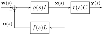
Figure 1: Block diagram of the closed-loop system $T(s)$ from the disturbance input $\mathbb{w}(s)$ to the performance output $\mathbb{y}(s)$ and the closed-loop system $H_{\mathbb{x}\mathbb{w}}(s)$ from $\mathbb{w}(s)$ to the position state $\mathbb{x}(s)$. The performance output $\mathbb{y}(s)$ is given by (3) if $r(s)=1$ and by (4) if $r(s)=s$.

In this section, we express the dynamics given in (1) and (2) in the frequency domain using an approach based on [33]. The framework, denoted in Figure 1, describes identical systems $g(s)$ receiving feedback that depends on an arbitrary transfer function $f(s)$ and the weighted graph Laplacian $L$ emitted by the network interconnection. Assuming that $\mathbb{x}(0)=\mathbb{v}(0)=0$ (we consider perturbations to the equilibrium), the closed-loop system from the input $\mathbb{w}$ to the position state $\mathbb{x}$ is given by

$$\left[(g(s)^{-1}I+f(s)L\right]\mathbb{x}(s)=\mathbb{w}(s),$$

which leads to

$$\mathbb{x}(s)=\left[(I+g(s)f(s)L\right]^{-1}g(s)\mathbb{w}(s)=:H_{\mathbb{x}\mathbb{w}}(s)\mathbb{w}(s),$$ (9)

where $H_{\mathbb{x}\mathbb{w}}(s)$ denotes the transfer function from the input $\mathbb{w}$ to the position state $\mathbb{x}$.

$L$ can be decomposed as $L=RJR^{-1}$, where $R\in\mathbb{C}^{n\times n}$ is invertible and $J\in\mathbb{C}^{n\times n}$ is in Jordan Canonical Form (JCF). This decomposition transforms (9) into

$$\mathbb{x}(s)=R\left[(I+g(s)f(s)J\right]^{-1}g(s)R^{-1}\mathbb{w}(s),$$

as shown by the block diagram in Figure 2. Defining $\mathbb{\tilde{x}}:=R^{-1}\mathbb{x}$ and $\mathbb{\tilde{w}}:=R^{-1}\mathbb{w}$, the transfer function from $\mathbb{\tilde{w}}$ to $\mathbb{\tilde{x}}$ is

$$H_{\mathbb{\tilde{x}}\mathbb{\tilde{w}}}(s)=\left[(I+g(s)f(s)J\right]^{-1}g(s),$$ (10)

where the following relationship holds

$$H_{\mathbb{x}\mathbb{w}}=RH_{\mathbb{\tilde{x}}\mathbb{\tilde{w}}}R^{-1}.$$ (11)

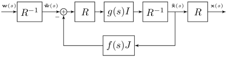
Figure 2: Application of a change of basis given by the Jordan decomposition $L=RJR^{-1}$ to the closed-loop system $H_{\mathbb{x}\mathbb{w}}(s)$. The feedback loop gives the closed-loop system $H_{\mathbb{\tilde{x}}\mathbb{\tilde{w}}}(s)$.

$J$ is composed of Jordan blocks $J_{k}$ associated with the eigenvalues $\lambda_{k}\in\mathbb{C}$ of $L$ for $k=1,\dots,m$:

$$J=\operatorname{blockdiag}{\left(J_{k}\right)_{1\leq k\leq m}},$$ (12)

where $J_{k}\in\mathbb{C}^{n_{k}\times n_{k}}$ and $\sum_{k=1}^{m}n_{k}=n$. Since $L$ is a Laplacian matrix, $L\mathbb{1}=\mathbb{0}$ with $\mathbb{1}$ denoting the vector of all ones therefore $J_{1}=\lambda_{1}=0$. Also $\operatorname{Re}\left[\lambda_{k}\right]>0$ for $k=2,\dots,m$ due to the fact that $\mathcal{G}$ has a globally reachable node [37, Theorem 7.4]. So (10) can be written as

$$H_{\mathbb{\tilde{x}}\mathbb{\tilde{w}}}(s)=\operatorname{blockdiag}{\left(H_{\mathbb{\tilde{x}}_{k}\mathbb{\tilde{w}}_{k}}(s)\right)_{1\leq k\leq m}},$$ (13)

where

$$H_{\mathbb{\tilde{x}}_{k}\mathbb{\tilde{w}}_{k}}(s)=\left[(I+g(s)f(s)J_{k}\right]^{-1}g(s).$$ (14)

Here, the vectors $\mathbb{\tilde{x}}_{k}=[\tilde{x}_{d_{k}+1},\dots,\tilde{x}_{d_{k}+n_{k}}]^{\intercal}$ and $\mathbb{\tilde{w}}_{k}~{}=~{}[\tilde{w}_{d_{k}+1},\dots,\tilde{w}_{d_{k}+n_{k}}]^{\intercal}$ respectively denote the position state and the input to the associated subsystem, with $d_{1}=0$ and $d_{k}=\sum_{i=1}^{k-1}n_{i}$ for $k=2,\dots,m$. An equivalent representation of the transfer function in (14) is given by the block diagram in Figure 3.

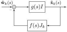
Figure 3: Block diagram of each subsystem $H_{\mathbb{\tilde{x}}_{k}\mathbb{\tilde{w}}_{k}}$ for $k=1,\dots,m$.

The following lemma describes the form of the transfer function in (14) which will be used to compute the performance metric (8) in what follows.

Lemma 1.

$H_{\mathbb{\tilde{x}}_{k}\mathbb{\tilde{w}}_{k}}(s)$ in (14) is an upper triangular Toeplitz matrix given by

$$H_{\mathbb{\tilde{x}}_{k}\mathbb{\tilde{w}}_{k}}(s)=\frac{1}{f(s)}\begin{bmatrix}h_{k}(s)&\dots&(-1)^{n_{k}-1}h_{k}(s)^{n_{k}}\\ &\ddots&\vdots\\ &&h_{k}(s)\end{bmatrix},$$

where $h_{k}(s)=\frac{g(s)f(s)}{1+\lambda_{k}g(s)f(s)}$.

Proof.

Using (14) and the definition of $J_{k}$

$$H_{\mathbb{\tilde{x}}_{k}\mathbb{\tilde{w}}_{k}}(s)=\begin{bmatrix}\frac{1+\lambda_{k}g(s)f(s)}{g(s)}&f(s)&&\\ &\ddots&\ddots&\\ &&\ddots&f(s)\\ &&&\frac{1+\lambda_{k}g(s)f(s)}{g(s)}\end{bmatrix}^{-1},$$

where factoring out $g(s)f(s)$ gives

$$H_{\mathbb{\tilde{x}}_{k}\mathbb{\tilde{w}}_{k}}(s)=\frac{1}{f(s)}\begin{bmatrix}h_{k}(s)^{-1}&1&&\\ &\ddots&\ddots&\\ &&\ddots&1\\ &&&h_{k}(s)^{-1}\end{bmatrix}^{-1}.$$ (15)

Using the inverse of the JCF in (15) yields the result. ∎

Remark 1.

The form of the closed-loop transfer function in Lemma 1 holds for arbitrary open-loop and feedback transfer functions $g(s)$ and $f(s)$, and therefore applies to a general class of networked dynamical systems.

We next apply Lemma 1 to the special cases of the single and double-integrator networks.

Corollary 1.

Consider the single-integrator network (1). Then, $H_{\mathbb{\tilde{x}}_{k}\mathbb{\tilde{w}}_{k}}(s)$ in (14) is an upper triangular Toeplitz matrix

$$H_{\mathbb{\tilde{x}}_{k}\mathbb{\tilde{w}}_{k}}(s)=\begin{bmatrix}h_{k}(s)&\dots&(-1)^{n_{k}-1}h_{k}(s)^{n_{k}}\\ &\ddots&\vdots\\ &&h_{k}(s)\end{bmatrix},$$

where $h_{k}(s)=\frac{1}{s+\lambda_{k}}$.

Proof.

Taking the Laplace transform of (1) leads to $g(s)=\frac{1}{s}$ and $f(s)=1$. Evaluating the result of Lemma 1 at these values gives the desired result. ∎

Corollary 2.

Consider the double-integrator network (2). Then, $H_{\mathbb{\tilde{x}}_{k}\mathbb{\tilde{w}}_{k}}(s)$ in (14) is an upper triangular Toeplitz matrix

$$H_{\mathbb{\tilde{x}}_{k}\mathbb{\tilde{w}}_{k}}(s)=\frac{1}{\gamma_{p}+s\gamma_{d}}\begin{bmatrix}h_{k}(s)&\dots&(-1)^{n_{k}-1}h_{k}(s)^{n_{k}}\\ &\ddots&\vdots\\ &&h_{k}(s)\end{bmatrix},$$

where $h_{k}(s)=\frac{\gamma_{p}+s\gamma_{d}}{s^{2}+(k_{d}+\gamma_{d}\lambda_{k})s+k_{p}+\gamma_{p}\lambda_{k}}$.

Proof.

Taking the Laplace transform of (2) leads to $g(s)~{}=~{}\frac{1}{s^{2}+k_{d}s+k_{p}}$ and $f(s)~{}=~{}\gamma_{p}+s\gamma_{d}$. Evaluating the result of Lemma 1 at these values gives the desired result. ∎

The transfer function from the input $\mathbb{w}$ to the velocity state $\mathbb{v}$ is given by $H_{\mathbb{v}\mathbb{w}}(s):=sH_{\mathbb{x}\mathbb{w}}(s)$ since $\mathbb{v}(s)=s\mathbb{x}(s)=sH_{\mathbb{x}\mathbb{w}}(s)\mathbb{w}(s).$ Therefore, the closed-loop transfer function $T(s)$ from the input $\mathbb{w}$ to the output $\mathbb{y}$ can be written as

$$T(s)=Cr(s)H_{\mathbb{x}\mathbb{w}}(s),$$ (16)

using the notation in Figure 1 and specifying $r(s)$ such that

$$T(s)= CH_{\mathbb{x}\mathbb{w}}(s), r(s)=1$$ (17)

$$T(s)= CH_{\mathbb{v}\mathbb{w}}(s), r(s)=s$$ . (18)

The cases (17) and (18) correspond to the outputs (3) and (4), respectively. We next provide necessary and sufficient conditions for the input-output stability of (17) and (18), which ensure the finiteness of the performance metric (8).

III-A Input-Output Stability

In this subsection we state necessary and sufficient conditions for the input-output stability of (17) and (18). The following assumption will be imposed throughout the paper to eliminate the unstable consensus mode of the Laplacian from the performance output.

Assumption 2.

The output matrix $C$ satisfies $C\mathbb{1}=\mathbb{0}$.

First, we apply the change of basis in (11) to the closed-loop system (16). Since $L\mathbb{1}=\mathbb{0}$, we can apply the partitioning

$$R=\begin{bmatrix}\alpha\mathbb{1}&\tilde{R}\end{bmatrix}\ \text{and}\ R^{-1}=\begin{bmatrix}\mathbb{q}_{1}&\tilde{Q}^{*}\end{bmatrix}^{*},$$ (19)

where $\alpha\in\mathbb{C}$, $\mathbb{q}_{1}^{*}\in\mathbb{C}^{1\times n}$ is the left eigenvector of $\lambda_{1}=0$, $\tilde{R}\in\mathbb{C}^{n\times n-1}$ and $\tilde{Q}\in\mathbb{C}^{n-1\times n}$. Substituting (11), (13) and (19) into (16) we obtain

$$T(s) =C\left(\alpha r(s)H_{\mathbb{\tilde{x}}_{1}\mathbb{\tilde{w}}_{1}}(s)\mathbb{1}\mathbb{q}_{1}^{*}+\tilde{R}\,\tilde{H}(s)\tilde{Q}\right)$$

$$=C\tilde{R}\,\tilde{H}(s)\tilde{Q},$$ (20)

where

$$\!\tilde{H}(s)\!=\!\operatorname{blockdiag}{(\tilde{H}_{k}(s))}\!:=\!r(s)\operatorname{blockdiag}{\left(H_{\mathbb{\tilde{x}}_{k}\mathbb{\tilde{w}}_{k}}(s)\right)},\!\!\!\!\!\!\!\!$$ (21)

for $k=2,\dots,m$ and we have used Assumption 2 and the fact that $H_{\mathbb{\tilde{x}}_{1}\mathbb{\tilde{w}}_{1}}(s)$ is a scalar. We can partition $\tilde{R}$ in (19) as

$$\tilde{R}=\begin{bmatrix}\tilde{R}_{2}&\dots&\tilde{R}_{m}\end{bmatrix},$$ (22)

which is in a form that conforms to (12). Then the columns of $\tilde{R}_{k}~{}\in~{}\mathbb{C}^{n\times n_{k}}$ are the right generalized eigenvectors associated with the Jordan block $J_{k}$ in (12) for $k=2,\dots,m$. This partitioning leads to the following useful definition.

Definition 1.

The set of observable indices $\mathcal{N}_{obsv}$ is given by

$$\mathcal{N}_{obsv}=\left\{k\in\{2,\dots,m\}\mid C\tilde{R}_{k}\neq 0\right\}.$$ (23)

We now state the stability conditions. We begin with the system $T$ in (17) for the single-integrator network (1).

Proposition 2.

Consider the single-integrator network (1). The system $T$ in (17) is input-output stable if and only if Assumption 2 holds [37, Theorem 7.4].

As we show next for the double-integrator network (2), stability of the observable modes is necessary and sufficient for the input-output stability of the system $T$ given by (17) or (18). For simplicity, we assume $L$ to be diagonalizable; the result can be extended by relaxing this assumption.

Proposition 3.

Consider the double-integrator network (2) and suppose that $L$ is diagonalizable and assumptions 1 and 2 hold. The system $T$ given by (17) or (18) is input-output stable if and only if

$$s^{2}+(k_{d}+\gamma_{d}\lambda_{k})s+k_{p}+\gamma_{p}\lambda_{k}=0$$ (24)

has solutions that satisfy $\operatorname{Re}(s)<0$ for all $k\in\mathcal{N}_{obsv}$.

Proof.

Using the block diagram in Figure 3 and the fact that $J_{k}=\lambda_{k}$ leads to the following realization for $H_{\mathbb{\tilde{x}}_{k}\mathbb{\tilde{w}}_{k}}$

$$\begin{bmatrix}\mathbb{\dot{\tilde{x}}}_{k}\\ \mathbb{\dot{\tilde{v}}}_{k}\end{bmatrix} =\underbrace{\begin{bmatrix}0&1\\ -k_{p}-\gamma_{p}\lambda_{k}&-k_{d}-\gamma_{d}\lambda_{k}\end{bmatrix}}_{\Lambda_{k}}\begin{bmatrix}\mathbb{\tilde{x}}_{k}\\ \mathbb{\tilde{v}}_{k}\end{bmatrix}+\begin{bmatrix}0\\ 1\end{bmatrix}\mathbb{\tilde{w}}_{k}$$

$$\mathbb{\tilde{y}}_{k} =\begin{bmatrix}1&0\end{bmatrix}\begin{bmatrix}\mathbb{\tilde{x}}_{k}\\ \mathbb{\tilde{v}}_{k}\end{bmatrix}=\mathbb{\tilde{x}}_{k}.$$ (25)

Since $L$ is diagonalizable, the partitioning of $\tilde{R}$ in (22) becomes $\tilde{R}=\begin{bmatrix}\mathbb{r}_{2}&\dots&\mathbb{r}_{n}\end{bmatrix}$. Using the block-diagonal form of $\tilde{H}(s)$ in (21) and the conformal partitioning $\tilde{Q}~{}=~{}\begin{bmatrix}\mathbb{q}_{2}&\dots&\mathbb{q}_{n}\end{bmatrix}^{*}$, (20) can be expressed in time-domain as

$$T(t)\ =\ C\sum_{k=2}^{n}\mathbb{r}_{k}\tilde{H}_{k}(t)\mathbb{q}_{k}^{*}\ =C\!\sum_{k\in\mathcal{N}_{obsv}}\!\!\!\!\mathbb{r}_{k}\tilde{H}_{k}(t)\mathbb{q}_{k}^{*}.$$

For (17), we can use (21) and the realization for $H_{\mathbb{\tilde{x}}_{k}\mathbb{\tilde{w}}_{k}}$ in (25) to re-write the equation above as

$$T(t)\ = \sum_{k\in\mathcal{N}_{obsv}}\!\!\!\!\begin{bmatrix}C\mathbb{r}_{k}&0\end{bmatrix}e^{\Lambda_{k}t}\begin{bmatrix}0\\ \mathbb{q}_{k}^{*}\end{bmatrix},$$

which has a realization

$$T(t)=\left(\begin{array}[]{c|c}\left[\begin{smallmatrix}\ddots&&\\ &\Lambda_{k}&\\ &&\ddots\end{smallmatrix}\right]&\left[\begin{smallmatrix}\vdots\\ \left[\begin{smallmatrix}0\\ \mathbb{q}_{k}^{*}\end{smallmatrix}\right]\\ \vdots\end{smallmatrix}\right]\\ \hline\cr\left[\begin{smallmatrix}\dots&\left[\begin{smallmatrix}C\mathbb{r}_{k}&0\end{smallmatrix}\right]&\dots\end{smallmatrix}\right]&0\end{array}\right),\quad k\in\mathcal{N}_{obsv}.$$ (26)

The associated observability matrix is given by

$$\mathcal{O}=\left[\begin{array}[]{c}\left[\begin{smallmatrix}\dots&\left[\begin{smallmatrix}C\mathbb{r}_{k}&0\end{smallmatrix}\right]&\dots\end{smallmatrix}\right]\\ \left[\begin{smallmatrix}\dots&\left[\begin{smallmatrix}C\mathbb{r}_{k}&0\end{smallmatrix}\right]\Lambda_{k}&\dots\end{smallmatrix}\right]\\ \vdots\\ \left[\begin{smallmatrix}\dots&\left[\begin{smallmatrix}C\mathbb{r}_{k}&0\end{smallmatrix}\right]\Lambda_{k}^{2|\mathcal{N}_{obsv}|-1}&\dots\end{smallmatrix}\right]\end{array}\right],$$ (27)

where $k\in\mathcal{N}_{obsv}$ and $|\mathcal{N}_{obsv}|$ denotes the cardinality of $\mathcal{N}_{obsv}$. Due to the form of $\Lambda_{k}$ in (25), we can see that $\begin{bmatrix}C\mathbb{r}_{k}&0\end{bmatrix}\Lambda_{k}=\begin{bmatrix}0&C\mathbb{r}_{k}\end{bmatrix}$. Then the first two block-rows of (27) imply that $\mathcal{O}$ is full rank if the vectors $C\mathbb{r}_{k}$ are linearly independent for $k\in\mathcal{N}_{obsv}$. For a proof by contradiction, assume that $C\mathbb{r}_{k}$ are linearly dependent, i.e. $\sum_{k\in\mathcal{N}_{obsv}}\alpha_{k}C\mathbb{r}_{k}=0$ where $\alpha_{k}$ is non-zero for some $k$. This implies that $\sum_{k\in\mathcal{N}_{obsv}}\alpha_{k}\mathbb{r}_{k}\in\ker\{C\}$, which can be expressed as a linear combination of the vectors that span $\ker\{C\}$. Then

$$\sum_{k\in\mathcal{N}_{obsv}}\alpha_{k}\mathbb{r}_{k}=-\!\!\sum_{k\in\{1,\dots,n\}\setminus\mathcal{N}_{obsv}}\!\!\alpha_{k}\mathbb{r}_{k}\Rightarrow\sum_{k=1}^{n}\alpha_{k}\mathbb{r}_{k}=0,$$

which would contradict the fact that $R$ is invertible. Therefore, $\mathcal{O}$ in (27) is full rank, so the realization in (26) is observable. By a similar argument we can prove the controllability, hence the minimality of (26). Therefore, the poles of $T(s)$ in (17) are given precisely by the eigenvalues of the system matrix in (26), which are determined by (24). Then $T(s)$ is input-output stable if and only if its poles are on the open left half-plane.

We now repeat the argument for (18) which is given by

$$T(t)\ = \sum_{k\in\mathcal{N}_{obsv}}\!\!\!\!\begin{bmatrix}0&C\mathbb{r}_{k}\end{bmatrix}e^{\Lambda_{k}t}\begin{bmatrix}0\\ \mathbb{q}_{k}^{*}\end{bmatrix}$$

in time-domain with a realization

$$T(t)=\left(\begin{array}[]{c|c}\left[\begin{smallmatrix}\ddots&&\\ &\Lambda_{k}&\\ &&\ddots\end{smallmatrix}\right]&\left[\begin{smallmatrix}\vdots\\ \left[\begin{smallmatrix}0\\ \mathbb{q}_{k}^{*}\end{smallmatrix}\right]\\ \vdots\end{smallmatrix}\right]\\ \hline\cr\left[\begin{smallmatrix}\dots&\left[\begin{smallmatrix}0&C\mathbb{r}_{k}\end{smallmatrix}\right]&\dots\end{smallmatrix}\right]&0\end{array}\right),\quad k\in\mathcal{N}_{obsv}.$$ (28)

The associated observability matrix is given by

$$\mathcal{O}=\left[\begin{array}[]{c}\left[\begin{smallmatrix}\dots&\left[\begin{smallmatrix}0&C\mathbb{r}_{k}\end{smallmatrix}\right]&\dots\end{smallmatrix}\right]\\ \left[\begin{smallmatrix}\dots&\left[\begin{smallmatrix}0&C\mathbb{r}_{k}\end{smallmatrix}\right]\Lambda_{k}&\dots\end{smallmatrix}\right]\\ \vdots\\ \left[\begin{smallmatrix}\dots&\left[\begin{smallmatrix}0&C\mathbb{r}_{k}\end{smallmatrix}\right]\Lambda_{k}^{2|\mathcal{N}_{obsv}|-1}&\dots\end{smallmatrix}\right]\end{array}\right],$$ (29)

where $k\in\mathcal{N}_{obsv}$. Since

$$\begin{bmatrix}0&C\mathbb{r}_{k}\end{bmatrix}\Lambda_{k}=C\mathbb{r}_{k}\begin{bmatrix}-k_{p}-\gamma_{p}\lambda_{k}&-k_{d}-\gamma_{d}\lambda_{k}\end{bmatrix},$$

and assumption 1 holds, (29) is full rank and (28) is observable, hence minimal. Therefore, the poles of $T(s)$ in (18) are given precisely by the eigenvalues of the system matrix in (28), which are determined by (24). Then $T(s)$ is input-output stable if and only if its poles are on the open left half-plane. ∎

Remark 2.

Assumption 2 can be relaxed for specific values of $k_{p}$ and $k_{d}$ for which the consensus modes become Hurwitz. If $k_{p}\neq 0$ and $k_{d}\neq 0$, the assumption can be relaxed for both (17) and (18) since $H_{\mathbb{\tilde{x}}_{1}\mathbb{\tilde{w}}_{1}}(s)=\frac{h_{1}(s)}{f(s)}=g(s)=\frac{1}{s^{2}+k_{d}s+k_{p}}$ and $H_{\mathbb{\tilde{v}}_{1}\mathbb{\tilde{w}}_{1}}(s)=sH_{\mathbb{\tilde{x}}_{1}\mathbb{\tilde{w}}_{1}}(s)=\frac{s}{s^{2}+k_{d}s+k_{p}}$ have stable poles by the Routh-Hurwitz criterion.

Similarly, one can relax the assumption for (18) but not for (17) if $k_{p}=0$ and $k_{d}\neq 0$ since $H_{\mathbb{\tilde{x}}_{1}\mathbb{\tilde{w}}_{1}}(s)=\frac{1}{s^{2}+k_{d}s}$ has a pole at $s=0$ but $H_{\mathbb{\tilde{v}}_{1}\mathbb{\tilde{w}}_{1}}(s)=\frac{s}{s^{2}+k_{d}s}=\frac{1}{s+k_{d}}$ has a stable pole. However for the sake of simplicity, we only consider performance metrics such that Assumption 2 is satisfied for both (17) and (18).

The stability condition in Proposition 3 can be restated as follows.

Proposition 4.

Consider the double-integrator network (2) and suppose that $L$ is diagonalizable and assumptions 1 and 2 hold. The system $T$ given by (17) or (18) is input-output stable if and only if

$$\alpha_{k}\phi_{k}^{2}+\beta_{k}\xi_{k}\phi_{k}-\beta_{k}^{2}>0\ \text{and}\ \phi_{k}>0,\ \ k\in\mathcal{N}_{obsv},$$ (30)

where $\alpha_{k}=k_{p}+\gamma_{p}\operatorname{Re}[\lambda_{k}]$, $\phi_{k}=k_{d}+\gamma_{d}\operatorname{Re}[\lambda_{k}]$, $\beta_{k}=\gamma_{p}\operatorname{Im}[\lambda_{k}]$ and $\xi_{k}=\gamma_{d}\operatorname{Im}[\lambda_{k}]$.

Proof.

The result follows from applying [38, Lemma 4] to Proposition 3. ∎

IV Performance over Arbitrary Digraphs

In this section, we use the block-diagonalization procedure outlined in Section III to derive closed-form expressions for the performance of the single and double-integrator networks (1) and (2) over arbitrary directed graphs that have at least one globally reachable node. Throughout the discussion we use both time and frequency domain representations, which simplifies the analysis.

First, we simplify (8) using the block-diagonal form of (13) and show that performance can be quantified as a linear combination of scalar integrals. These integrals can be interpreted as $\mathcal{L}_{2}$ scalar products of the elements of the closed-loop impulse response function matrix blocks $H_{\mathbb{\tilde{x}}_{k}\mathbb{\tilde{w}}_{k}}(t)$ and $H_{\mathbb{\tilde{v}}_{k}\mathbb{\tilde{w}}_{k}}(t)$.

Combining (8) and (20), the performance metric in (8) can be written as

$$P=\int_{0}^{\infty}\mathbb{w}_{0}^{*}\tilde{Q}^{*}\tilde{H}(t)^{*}\tilde{N}\tilde{H}(t)\tilde{Q}\mathbb{w}_{0}dt,$$ (31)

where $\tilde{N}=\tilde{R}^{*}C^{*}C\tilde{R}$ and $\tilde{H}$ is defined as in (21) with

$$\tilde{H}_{k}(s)=\begin{bmatrix}\tilde{h}_{11}^{(k)}(s)&\dots&\tilde{h}_{1,n_{k}}^{(k)}(s)\\ &\ddots&\vdots\\ &&\tilde{h}_{n_{k},n_{k}}^{(k)}(s)\end{bmatrix}$$ (32)

for $k=2,\dots,m$. The upper triangular form of (32) is given in Lemma 1. Since

$$M:=C^{*}C$$ (33)

is a symmetric matrix, it is unitarily diagonalizable, i.e.

$$\!M=\Theta W\Theta^{*},\ \ W=\operatorname{diag}{(\mu_{i})_{1\leq i\leq n}}\in\mathbb{R}^{n\times n}\!,\ \ \text{and}\ \ \Theta\Theta^{*}=I,$$

therefore $\tilde{N}=\tilde{R}^{*}\Theta W\Theta^{*}\tilde{R}$. Using Assumption 2 and assuming without loss of generality that $\mu_{1}=0$ is associated with the eigenvector $\boldsymbol{\theta}_{1}=\frac{1}{\sqrt{n}}\mathbb{1}$, we can state $\tilde{N}$ element-wise as

$$(\tilde{N})_{\eta-1,\kappa-1}=\sum_{l=2}^{n}\langle\boldsymbol{\theta}_{l},\mathbb{r}_{\eta}\rangle\langle\mathbb{r}_{\kappa},\boldsymbol{\theta}_{l}\rangle\mu_{l}=:\nu_{\eta,\kappa}$$ (34)

for $\eta,\kappa=2,\dots,n$, where $\langle\boldsymbol{\theta}_{l},\mathbb{r}_{\eta}\rangle=\mathbb{r}_{\eta}^{*}\boldsymbol{\theta}_{l}$, $\mathbb{r}_{\kappa}$ and $\boldsymbol{\theta}_{l}$ denote respectively the columns $\kappa$ and $l$ of $\tilde{R}$ and $\Theta$.

Using this notation, (31) can be written in terms of the scalar products between the elements of $\tilde{H}_{k}(t)$, which are given by the element-wise inverse Laplace transforms of (32).

Lemma 2.

The performance metric $P$ in (31) is given by

$$P=\operatorname{tr}{(\Sigma_{Q}\Psi)},$$ (35)

where

$$\Sigma_{Q}=\tilde{Q}\Sigma_{0}\tilde{Q}^{*},\,\Sigma_{0}=\mathbb{w}_{0}\mathbb{w}_{0}^{*},$$ (36)

and the matrix $\Psi$ is partitioned as $\Psi=\left[\Psi_{kl}\right]_{2\leq k,l\leq m}.$

Furthermore, the entry $(q,b)$ of the matrix $\Psi_{kl}$ for $k,l~{}=~{}2,\dots,m$ is given by

$$\left[\Psi_{kl}\right]_{qb}=\sum_{p=1}^{q}\sum_{a=1}^{b}\nu_{d_{k}+p,d_{l}+a}\left\langle\tilde{h}_{ab}^{(l)}(t),\tilde{h}_{pq}^{(k)}(t)\right\rangle_{\mathcal{L}_{2}},$$ (37)

where

$$\left\langle\tilde{h}_{ab}^{(l)}(t),\tilde{h}_{pq}^{(k)}(t)\right\rangle_{\mathcal{L}_{2}}=\int_{0}^{\infty}\overline{\tilde{h}_{pq}^{(k)}(t)}\tilde{h}_{ab}^{(l)}(t)dt.$$ (38)

Here the indices $q=1,\dots,n_{k}$ and $b=1,\dots,n_{l}$ are determined by the Jordan block sizes $n_{k}$ and $n_{l}$. Terms of the form in (34) appear in the summand of (37) and their indices take values larger than the sum of the previous Jordan block sizes, namely $d_{k}=\sum_{i=1}^{k-1}n_{i}$ and $d_{l}=\sum_{i=1}^{l-1}n_{i}$.

Remark 3.

For the special case in which $L$ is diagonalizable each Jordan block is a scalar, i.e. $n_{k}=1$, and (37) leads to

$$\Psi_{kl}=\nu_{kl}\left\langle\tilde{h}^{(l)}(t),\tilde{h}^{(k)}(t)\right\rangle_{\mathcal{L}_{2}}.$$

Here we dropped the subscripts of $\tilde{h}_{pq}^{(k)}$ for simplicity. The case with diagonalizable $L$ was studied in [33, 34] and Lemma 2 provides a generalization to the case of arbitrary Jordan block size $n_{k}$ for $k=2,\dots,m$.

Proof of Lemma 2.

Taking the trace of both sides of (31) and using the permutation property of the trace, we have $P=\operatorname{tr}\left(\tilde{Q}\mathbb{w}_{0}\mathbb{w}_{0}^{*}\tilde{Q}^{*}\Psi\right),$ where $\Psi(t)=\int_{0}^{\infty}\tilde{H}(t)^{*}\tilde{N}\tilde{H}(t)dt$. Partitioning $\tilde{N}$ conformally so that its $(k,l)$ block is given by $\tilde{N}_{kl}$, one can write

$$\Psi_{kl}=\int_{0}^{\infty}\tilde{H}_{k}(t)^{*}\tilde{N}_{kl}\tilde{H}_{l}(t)dt,$$ (39)

for $k,l=2,\dots,m$. Direct multiplication of the matrices in the integral argument and interchanging the order of integration with the summation gives the desired result. ∎

Remark 4.

Since $\tilde{N}=\tilde{N}^{*}$, i.e. $\tilde{N}_{kl}=\tilde{N}_{lk}^{*}$, (39) leads to $\Psi_{kl}=\Psi_{lk}^{*}$, therefore $\Psi$ is Hermitian. The fact that $\Sigma_{Q}$ in (36) is also Hermitian leads to $\operatorname{tr}{(\Sigma_{Q}\Psi)}=\operatorname{tr}{\left[(\Sigma_{Q}\Psi)^{*}\right]}=\overline{\operatorname{tr}{(\Sigma_{Q}\Psi)}},$ which verifies that $P$ in (35) is real as expected.

As Lemma 2 indicates, (35) can be expressed in closed-form if the integral in (38) can be evaluated. In what follows, we derive time-domain realizations for the transfer functions $\tilde{h}_{pq}^{(k)}(s)$ in (32), which enables the evaluation of this integral. This leads to our first major contribution, which we state next for single and double-integrator networks (1) and (2).

IV-A Performance of Single-Integrator Networks

We now present the main result of this section for the single-integrator network (1). The following result provides a closed-form solution for the performance metric $P$ in (5).

Theorem 1.

Consider the single-integrator network (1). The performance metric $P$ in (5) for the system $T$ given by (17) is $P=\operatorname{tr}{(\Sigma_{Q}\Psi)}.$ The elements of $\Psi$ are defined in (37) and the scalar product in (38) is given by

$$\left\langle\tilde{h}_{ab}^{(l)}(t),\tilde{h}_{pq}^{(k)}(t)\right\rangle_{\mathcal{L}_{2}}=\frac{{(-1)}^{b-a+q-p}\Phi}{{\left(\overline{\lambda_{k}}+\lambda_{l}\right)}^{b-a+q-p+1}},$$ (40)

where $\Phi=\frac{(b-a+q-p)!}{(b-a)!(q-p)!}$.

Proof.

Using the result of Corollary 1 and the notation in (32)

$$\tilde{h}_{pq}^{(k)}(s)={(-1)}^{q-p}\frac{1}{{\left(s+\lambda_{k}\right)}^{q-p+1}}.$$

Here, $\frac{1}{{\left(s+\lambda_{k}\right)}^{q-p+1}}$ has the following realization $\left(\mathcal{A}_{k,\delta},\mathcal{B}_{k,\delta},\mathcal{C}_{k,\delta}\right)$ in JCF

$$\mathcal{A}_{k,\delta}=\mathcal{J}(-\lambda_{k},\delta),$$ (41)

$$\mathcal{B}_{k,\delta}=\bigg{[}\underbrace{\begin{matrix}0&\dots&1\end{matrix}}_{1\times\delta}\bigg{]}^{\intercal},\mathcal{C}_{k,\delta}=\bigg{[}\underbrace{\begin{matrix}1&\dots&0\end{matrix}}_{1\times\delta}\bigg{]},$$

where $\mathcal{J}(-\lambda_{k},\delta)$ denotes the size-$\delta$ Jordan block with the eigenvalue $-\lambda_{k}$ and $\delta=q-p+1$. Then, $\tilde{h}_{pq}^{(k)}(t)$ is given by

$$\tilde{h}_{pq}^{(k)}(t)={(-1)}^{q-p}C_{k,\delta}e^{A_{k,\delta}t}B_{k,\delta}.$$ (42)

where

$$e^{A_{k,\delta}t}=e^{\mathcal{J}(-\lambda_{k},\delta)t}=e^{-\lambda_{k}t}\begin{bmatrix}1&t&\dots&\frac{t^{(\delta-1)}}{(\delta-1)!}\\ &\ddots&\ddots&\vdots\\ &&&t\\ &&&1\end{bmatrix}.$$ (43)

Combining (41) and (42) leads to

$$\tilde{h}_{pq}^{(k)}(t)={(-1)}^{q-p}e^{-\lambda_{k}t}\frac{t^{q-p}}{(q-p)!}.$$

The proof is completed by evaluating the integral in (38) using the fact that $\int_{0}^{\infty}t^{n}e^{-\lambda t}dt=\frac{n!}{\lambda^{n+1}}$ for $\lambda\in\mathbb{C}$, $\operatorname{Re}[\lambda]>0$. ∎

The denominator of the right-hand side of (40) is given by a power of the sum of the graph Laplacian eigenvalues that are associated with possibly distinct Jordan blocks $k$ and $l$. The power of this term depends on the Jordan block sizes $n_{k}$ and $n_{l}$ through the indices $q$ and $b$ and it increases as the Jordan block size increases. This indicates that performance is affected not only by the network size, but also by the graph Laplacian spectrum and the size of the individual Jordan blocks.

We next present the analogous result for the double-integrator network (2).

IV-B Performance of Double-Integrator Networks

We now provide the closed-form solution for the performance metric $P$ in (5) for the double-integrator network (2). A similar approach to the one in Theorem 1 is taken but the computation of the impulse response functions $\tilde{h}_{pq}^{(k)}(t)$ is more involved. We compute these functions through Lemmas 6 and 7 in the Appendix. Then by evaluating the integral in (38), the result of this subsection is stated as follows.

Theorem 2.

Consider the double-integrator network (2). Let $\rho_{1}^{(k)}$ and $\rho_{2}^{(k)}$ denote the roots of

$$s^{2}+(k_{d}+\gamma_{d}\lambda_{k})s+k_{p}+\gamma_{p}\lambda_{k}=0.$$ (44)

The performance metric $P$ in (5) for the system $T$ given by (17) or (18) is $P=\operatorname{tr}{(\Sigma_{Q}\Psi)}$, where $\Psi$ is given element-wise by (37) and the scalar product in (38) is as follows:

If $\rho_{1}^{(k)}\neq\rho_{2}^{(k)}$ and $\rho_{1}^{(l)}\neq\rho_{2}^{(l)}$

$$\left\langle\tilde{h}_{ab}^{(l)}(t),\tilde{h}_{pq}^{(k)}(t)\right\rangle_{\mathcal{L}_{2}}=\sum_{\zeta=1}^{\sigma}\sum_{r=1}^{\upsilon}\frac{\Phi_{\zeta r}(\sigma,\upsilon)\overline{c_{\zeta}^{(k)}}c_{r}^{(l)}}{{\left(\overline{\rho_{1}^{(k)}}+\rho_{1}^{(l)}\right)}^{\sigma+\upsilon-\zeta-r+1}}$$

$$+\frac{\Phi_{\zeta r}(\sigma,\upsilon)\overline{c_{\zeta}^{(k)}}c_{r+\upsilon}^{(l)}}{{\left(\overline{\rho_{1}^{(k)}}+\rho_{2}^{(l)}\right)}^{\sigma+\upsilon-\zeta-r+1}}\ +\ \frac{\Phi_{\zeta r}(\sigma,\upsilon)\overline{c_{\zeta+\sigma}^{(k)}}c_{r}^{(l)}}{{\left(\overline{\rho_{2}^{(k)}}+\rho_{1}^{(l)}\right)}^{\sigma+\upsilon-\zeta-r+1}}$$

$$+\frac{\Phi_{\zeta r}(\sigma,\upsilon)\overline{c_{\zeta+\sigma}^{(k)}}c_{r+\upsilon}^{(l)}}{{\left(\overline{\rho_{2}^{(k)}}+\rho_{2}^{(l)}\right)}^{\sigma+\upsilon-\zeta-r+1}},$$ (45)

If $\rho_{1}^{(k)}\neq\rho_{2}^{(k)}$ and $\rho_{1}^{(l)}=\rho_{2}^{(l)}=\rho^{(l)}$

$$\!\!\!\!\left\langle\tilde{h}_{ab}^{(l)}(t),\tilde{h}_{pq}^{(k)}(t)\right\rangle_{\mathcal{L}_{2}} =\sum_{\zeta=1}^{\sigma}\sum_{r=1}^{2\upsilon}\frac{{(-1)}^{\upsilon}\Phi_{\zeta r}(\sigma,2\upsilon)\overline{c_{\zeta}^{(k)}}c_{r}^{(l)}}{{\left(\overline{\rho_{1}^{(k)}}+\rho^{(l)}\right)}^{\sigma+2\upsilon-\zeta-r+1}}$$

$$+\frac{{(-1)}^{\upsilon}\Phi_{\zeta r}(\sigma,2\upsilon)\overline{c_{\zeta+\sigma}^{(k)}}c_{r}^{(l)}}{{\left(\overline{\rho_{2}^{(k)}}+\rho^{(l)}\right)}^{\sigma+2\upsilon-\zeta-r+1}},$$ (46)

If $\rho_{1}^{(k)}=\rho_{2}^{(k)}=\rho^{(k)}$ and $\rho_{1}^{(l)}=\rho_{2}^{(l)}=\rho^{(l)}$

$$\!\!\left\langle\tilde{h}_{ab}^{(l)}(t),\tilde{h}_{pq}^{(k)}(t)\right\rangle_{\mathcal{L}_{2}}\!=\!\sum_{\zeta=1}^{2\sigma}\sum_{r=1}^{2\upsilon}\frac{{(-1)}^{\sigma+\upsilon}\Phi_{\zeta r}(2\sigma,2\upsilon)\overline{c_{\zeta}^{(k)}}c_{r}^{(l)}}{{\left(\overline{\rho^{(k)}}+\rho^{(l)}\right)}^{2\sigma+2\upsilon-\zeta-r+1}}\!,$$ (47)

where $\sigma=q-p+1$, $\upsilon=b-a+1$ and $\Phi_{\zeta r}(\sigma,\upsilon)~{}=~{}{(-1)}^{1-\zeta-r}\frac{(\sigma+\upsilon-\zeta-r)!}{(\sigma-\zeta)!(\upsilon-r)!}$.

The coefficients $c_{\zeta}^{(k)}$ are given in the Appendix by Lemma 6 if $\rho_{1}^{(k)}\neq\rho_{2}^{(k)}$ and by Lemma 7 if $\rho_{1}^{(k)}=\rho_{2}^{(k)}$.

Remark 5.

For double-integrator networks, the scalar products in (2) - (47) depend on both the control gains and the eigenvalues of $L$, via the roots of (44) and the coefficients $c_{\zeta}^{(k)}$. In contrast, for single-integrator networks, eigenvalues of $L$ appear explicitly in the analogous expression in (40).

Proof of Theorem 2.

Using the result of Corollary 2, the notation in (32) and (90), $\tilde{h}_{pq}^{(k)}(t)$ is given by

$$\tilde{h}_{pq}^{(k)}(t)={(-1)}^{\sigma-1}\Omega_{k,\sigma}(t).$$ (48)

If $\rho_{1}^{(k)}\neq\rho_{2}^{(k)}$, the realization in (91) can be used to calculate

$$\Omega_{k,\sigma}(t)=C_{k,\sigma}e^{A_{k,\sigma}t}B_{k,\sigma},\\$$

where $e^{A_{k,\sigma}t}=\operatorname{blockdiag}{\left(e^{\mathcal{J}(\rho_{i}^{(k)},\,\sigma)t}\right)}_{i=1,2}$ and $e^{\mathcal{J}(\rho_{i}^{(k)},\,\sigma)t}$ can be expanded as in (43). Then, using (48) and the definitions of $C_{k,\sigma}$ and $B_{k,\sigma}$ in (91)

$$\tilde{h}_{pq}^{(k)}(t)={(-1)}^{\sigma-1}\sum_{\zeta=1}^{\sigma}\left(c_{\zeta}^{(k)}e^{\rho_{1}^{(k)}t}+c_{\zeta+\sigma}^{(k)}e^{\rho_{2}^{(k)}t}\right)\frac{t^{\sigma-\zeta}}{(\sigma-\zeta)!}.$$

If $\rho_{1}^{(k)}=\rho_{2}^{(k)}=\rho^{(k)}$, a similar argument combined with (100) leads to

$$\tilde{h}_{pq}^{(k)}(t)={(-1)}^{\sigma-1}\sum_{\zeta=1}^{2\sigma}c_{\zeta}^{(k)}e^{\rho^{(k)}t}\frac{t^{2\sigma-\zeta}}{(2\sigma-\zeta)!}.$$

The proof is completed by evaluating the integral in (38) using the fact that $\int_{0}^{\infty}t^{n}e^{\lambda t}dt={(-1)}^{n+1}\frac{n!}{\lambda^{n+1}}$ for $\lambda\in\mathbb{C}$, $\operatorname{Re}[\lambda]~{}<~{}0$. ∎

Theorems 1 and 2 provide closed-form solutions for the performance metric (5) which consist of terms that: (a) are geometric, i.e. terms that depend on the input direction, the eigenvalues and the eigenvectors of $M$ in (33) and the eigenvectors of $L$ as in (34) and (36); and (b) terms that depend on the closed-loop dynamics of the system, as in (38). Overall, performance is given by a linear combination of the entries of the matrix $\Psi$ in (37), weighted by the entries of the matrix $\Sigma_{Q}$ in (36). Therefore, in the most general case, it is not straightforward to deduce the individual effect of properties such as network size, graph topology and the spectrum of the output matrix for an arbitrary system.

In the next section, we study special cases to provide insight on the effect of edge directionality on performance.

V Digraphs with Diagonalizable Laplacian Matrices

We now consider the class of graphs that emit diagonalizable Laplacian matrices; and its subclass of normal Laplacian matrices. The closed-form solutions derived here will be used in sections VI and VII to provide further insights on the results of the last section. Namely, we will show that performance is determined by the interplay between edge directionality and control strategy (judicious selection of control gains).

V-A Single-Integrator Networks

The following theorem provides the main result of this section for the single-integrator network (1).

Theorem 3 (Single-Integrator, Diagonalizable Laplacian).

Consider the single-integrator network (1) and suppose that $L$ is diagonalizable. Then, the metric $P$ in (5) for the system $T$ given by (17) is $P=\operatorname{tr}{(\Sigma_{Q}\Psi)}$, where $\mathbb{j}^{2}=-1$ and

$$\Psi_{kl}=\nu_{kl}\frac{\operatorname{Re}[\lambda_{k}]+\operatorname{Re}[\lambda_{l}]+\mathbb{j}(\operatorname{Im}[\lambda_{k}]-\operatorname{Im}[\lambda_{l}])}{(\operatorname{Re}[\lambda_{k}]+\operatorname{Re}[\lambda_{l}])^{2}+(\operatorname{Im}[\lambda_{k}]-\operatorname{Im}[\lambda_{l}])^{2}}.$$ (49)

Proof.

The fact that $L$ is diagonalizable leads to $m=n$, i.e. all Jordan blocks are scalars. Then using (37) from Lemma 2, we have $\Psi_{kl}=\nu_{kl}\left\langle\tilde{h}_{11}^{(l)}(t),\tilde{h}_{11}^{(k)}(t)\right\rangle_{\mathcal{L}_{2}}$. Also, (40) from Theorem 1 gives $\left\langle\tilde{h}_{11}^{(l)}(t),\tilde{h}_{11}^{(k)}(t)\right\rangle_{\mathcal{L}_{2}}=\frac{1}{\overline{\lambda_{k}}+\lambda_{l}}.$ Combining these facts and re-arranging terms yields the result. ∎

Note that the diagonal terms $\Psi_{kk}$ are real and the cross-terms $\Psi_{kl}$ for $k\neq l$ are possibly imaginary in (49). However, $P$ is guaranteed to be real due to Remark 4.

Normal Laplacian Matrices

We next focus on systems over digraphs that emit normal weighted Laplacian matrices. First recall Definition 1, which introduced the set of observable indices $\mathcal{N}_{obsv}$ in (23). If $L$ is normal therefore diagonalizable, we can re-state this set as

$$\mathcal{N}_{obsv}=\left\{k\in\{2,\dots,n\}\mid C\mathbb{r}_{k}\neq 0\right\},$$

recalling that $\mathbb{r}_{k}$ denote the right eigenvectors of $L$ as defined in (19). We now present two lemmas that will be useful in proving the upcoming results.

Lemma 3.

For $k\in\{2,\dots,n\}$, the eigenvalue-eigenvector pair $(\mu_{k},\boldsymbol{\theta}_{k})$ of $M$ in (33) satisfies $\mu_{k}=0$ if and only if $C\boldsymbol{\theta}_{k}=0$.

Proof.

Assume for any $k\in\{2,\dots,n\}$ that $\mu_{k}=0$. Then $0=M\boldsymbol{\theta}_{k}=C^{T}C\boldsymbol{\theta}_{k}$. This implies that the vector $C\boldsymbol{\theta}_{k}$ is in the left nullspace of $C$, therefore is orthogonal to the column space of $C$. But $C\boldsymbol{\theta}_{k}$ also has to be in the column space of $C$ therefore $C\boldsymbol{\theta}_{k}=0$.

Conversely, if $C\boldsymbol{\theta}_{k}=0$ for any $k\in\{2,\dots,n\}$, then $0~{}=~{}M\boldsymbol{\theta}_{k}=\mu_{k}\boldsymbol{\theta}_{k}$ which gives $\mu_{k}=0$ since $\boldsymbol{\theta}_{k}\neq 0$. ∎

Lemma 4.

Suppose that $L$ is normal. For $k\in\{2,\dots,n\}$, $\nu_{kk}$ in (34) satisfies

1. $\nu_{kk}=0$ if and only if $k\notin\mathcal{N}_{obsv}$.

2. $\nu_{kk}>0$ if and only if $k\in\mathcal{N}_{obsv}$.

Proof.

Normality of $L$ means that it is unitarily diagonalizable, therefore $R^{-1}={R}^{*}$. We also recall that $M$ in (33) is symmetric, therefore unitarily diagonalizable. Therefore $\mathbb{r}_{1}=\boldsymbol{\theta}_{1}=\frac{1}{\sqrt{n}}\boldsymbol{1}$ and it holds that $\mathbb{r}_{k},\boldsymbol{\theta}_{l}\in\operatorname{span}\{\boldsymbol{1}\}^{\bot}\subset\mathbb{C}^{n}$ for $k,l\in~{}\{2,\dots,n\}$. So, we have $\mathbb{r}_{k}=\sum_{i=2}^{n}\chi_{i}^{k}\boldsymbol{\theta}_{i}$ with constants $\chi_{i}^{k}\in~{}\mathbb{C}$ for $k\in\{2,\dots,n\}$.

Given any $k\in\{2,\dots,n\}$, it follows from (34) and Lemma 3 that $\nu_{kk}=0$ if and only if $\left\langle\boldsymbol{\theta}_{l},\mathbb{r}_{k}\right\rangle=0$ for all $l\in~{}\{2,\dots,n\}$ such that $C\boldsymbol{\theta}_{l}\neq 0$. Combining the preceding arguments leads to

$$\nu_{kk}=0\ \Leftrightarrow\ \left(\sum_{i=2}^{n}\overline{\chi_{i}^{k}}\boldsymbol{\theta}_{i}^{*}\right)\boldsymbol{\theta}_{l}=0,\ l\in\{2,\dots,n\},\ C\boldsymbol{\theta}_{l}\neq 0,$$

which is equivalent to having $\chi_{l}^{k}=0$ for such $l$, due to the orthonormality of $\boldsymbol{\theta}_{l}$. In other words, $\nu_{kk}=0\ \Leftrightarrow\ \mathbb{r}_{k}\!\!~{}=~{}\!\!\!\!\sum\limits_{\begin{subarray}{c}C\boldsymbol{\theta}_{i}=0,\ i\in\{2,\dots,n\}\end{subarray}}\!\!\chi_{i}^{k}\boldsymbol{\theta}_{i}\ \Leftrightarrow\ C\mathbb{r}_{k}=0,$ which proves the first result. Since $M$ in (33) is postive semi-definite, $\nu_{kk}$ for $k\in\{2,\dots,n\}$ is given by a summation in (34) with each summand being non-negative. So, $\nu_{kk}\geq 0$ and the first result implies the second result. ∎

Theorem 3 leads to the following result for normal Laplacian matrices.

Corollary 3 (Single-Integrator, Normal Laplacian).

Consider the single-integrator network (1). Suppose that $L$ is normal and the input $\mathbb{w}_{0}$ has unit covariance, i.e. $E\left[\Sigma_{0}\right]=I$. Then, the expectation of the metric $P$ in (5) for the system $T$ given by (17) is

$$E\left[P\right]=\lVert T\rVert_{\mathcal{H}_{2}}^{2}=\sum_{k\in\mathcal{N}_{obsv}}\nu_{kk}\frac{1}{2\operatorname{Re}[\lambda_{k}]}.$$ (50)

Proof.

Orthonormality of $\mathbb{r}_{j}$ for $j=1,\dots,n$ yields $E\left[\Sigma_{Q}\right]~{}=~{}I$ and leads to $E\left[P\right]=\sum_{k=2}^{n}\Psi_{kk}$ due to Theorem 3. We note that this simplifies to (50) by using (49), Proposition 1 and Lemma 4. ∎

Although Corollary 3 is a special case of Theorem 3, and consequently Theorem 1, it generalizes [5, Proposition 1] to performance metrics with arbitrary output matrices.

V-B Double-Integrator Networks

Next we present the main result of this section for the double-integrator network (2).

Theorem 4 (Double-Integrator, Diagonalizable Laplacian).

Consider the double-integrator network (2). Suppose that $L$ is diagonalizable. The performance metric $P$ in (5) is $P=\operatorname{tr}{(\Sigma_{Q}\Psi)}$, where

$$\Psi_{kk}=\nu_{kk}\frac{\phi_{k}}{2(\alpha_{k}\phi_{k}^{2}+\beta_{k}\xi_{k}\phi_{k}-\beta_{k}^{2})}$$ (51)

for the position-based output, i.e. system $T$ given by (17) and

$$\Psi_{kk}=\nu_{kk}\frac{\xi_{k}\beta_{k}+\phi_{k}\alpha_{k}}{2(\alpha_{k}\phi_{k}^{2}+\beta_{k}\xi_{k}\phi_{k}-\beta_{k}^{2})}$$ (52)

for the velocity-based output, i.e. system $T$ given by (18); where $\alpha_{k}=k_{p}+\gamma_{p}\operatorname{Re}[\lambda_{k}]$, $\phi_{k}=k_{d}+\gamma_{d}\operatorname{Re}[\lambda_{k}]$, $\beta_{k}~{}=~{}\gamma_{p}\operatorname{Im}[\lambda_{k}]$ and $\xi_{k}=\gamma_{d}\operatorname{Im}[\lambda_{k}]$.

Remark 6.

Here, the cross-terms $\Psi_{kl}$ for $k\neq l$ are not given explicitly for brevity. A Gramian computation as in [33, 34] would give $\Psi_{kl}$ in closed-form for $k\neq l$, which is not tractable due to the number of terms involved. To gain some insight from the computation, we focus on the diagonal terms which are the only required ones when $\Sigma_{Q}$ in (36) is diagonal.

Proof of Theorem 4.

The fact that $L$ is diagonalizable leads to $m=n$, i.e. all Jordan blocks are scalars. Then, using (37) from Lemma 2 we have $\Psi_{kl}=\nu_{kl}\left\langle\tilde{h}_{11}^{(l)}(t),\tilde{h}_{11}^{(k)}(t)\right\rangle_{\mathcal{L}_{2}}.$ First consider the position-based performance metric, i.e. the system $T$ given by (17). Due to (48) from the proof of Theorem 2 and (90), $\tilde{h}_{11}^{(k)}(s)=\frac{1}{s^{2}+(k_{d}+\gamma_{d}\lambda_{k})s+k_{p}+\gamma_{p}\lambda_{k}}$, which has the realization $\left(\mathcal{A}_{k},\mathcal{B}_{k},\mathcal{C}_{k}\right)$ in controllable canonical form given by $\mathcal{A}_{k}=\left[\begin{smallmatrix}0&1\\ -k_{p}-\gamma_{p}\lambda_{k}&-k_{d}-\gamma_{d}\lambda_{k}\end{smallmatrix}\right]$, $\mathcal{B}_{k}=\begin{bmatrix}0&1\end{bmatrix}^{\intercal}$ and $\mathcal{C}_{k}=\begin{bmatrix}1&0\end{bmatrix}$. If $k=l$, performing a standard computation, $\left\langle\tilde{h}_{11}^{(k)}(t),\tilde{h}_{11}^{(k)}(t)\right\rangle_{\mathcal{L}_{2}}=\mathcal{B}_{k}^{\intercal}\mathcal{X}_{k}\mathcal{B}_{k}$, where $\mathcal{X}_{k}$ satisfies the Lyapunov equation $\mathcal{A}_{k}^{*}\mathcal{X}_{k}+\mathcal{X}_{k}\mathcal{A}_{k}=-\mathcal{C}_{k}^{*}\mathcal{C}_{k}$. Then we get

$$\left\langle\tilde{h}_{11}^{(k)}(t),\tilde{h}_{11}^{(k)}(t)\right\rangle_{\mathcal{L}_{2}}=\frac{\phi_{k}}{2(\alpha_{k}\phi_{k}^{2}+\beta_{k}\xi_{k}\phi_{k}-\beta_{k}^{2})}.$$

Considering the velocity-based performance metric, i.e. the system $T$ given by (18) and using (48) and (90) we have $\tilde{h}_{11}^{(k)}(s)=\frac{s}{s^{2}+(k_{d}+\gamma_{d}\lambda_{k})s+k_{p}+\gamma_{p}\lambda_{k}}$, so that $\mathcal{A}_{k}$ and $\mathcal{B}_{k}$ are the same but $\mathcal{C}_{k}=\begin{bmatrix}0&1\end{bmatrix}$. If $k=l$, solving the Lyapunov equation leads to

$$\left\langle\tilde{h}_{11}^{(k)}(t),\tilde{h}_{11}^{(k)}(t)\right\rangle_{\mathcal{L}_{2}}=\frac{\xi_{k}\beta_{k}+\phi_{k}\alpha_{k}}{2(\alpha_{k}\phi_{k}^{2}+\beta_{k}\xi_{k}\phi_{k}-\beta_{k}^{2})}.\quad\mbox{\qed}\!\!\!\!\!\!\!\!\!\!\!\!$$

If we further assume real eigenvalues, we obtain a result similar to the one in [33, 34] for diagonalizable Laplacians.

Corollary 4 (Double-Integrator, Diagonalizable Laplacian with Real Eigenvalues).

Consider the double-integrator network (2). Suppose that $L$ is diagonalizable and has real eigenvalues. Then

$$\Psi_{kl}=\nu_{kl}\frac{2k_{d}+\gamma_{d}(\lambda_{k}+\lambda_{l})}{\Psi_{kl}^{denom}},$$ (53)

for the position-based output, i.e. system $T$ given by (17) and

$$\Psi_{kl}=\nu_{kl}\frac{(k_{p}+\gamma_{p}\lambda_{l})(k_{d}+\gamma_{d}\lambda_{k})+(k_{p}+\gamma_{p}\lambda_{k})(k_{d}+\gamma_{d}\lambda_{l})}{\Psi_{kl}^{denom}}$$ (54)

for the velocity-based output, i.e. system $T$ given by (18), where

$$\Psi_{kl}^{denom}\,\, =\,\,(k_{d}+\gamma_{d}\lambda_{k})(k_{d}+\gamma_{d}\lambda_{l})(2k_{p}+\gamma_{p}(\lambda_{k}+\lambda_{l}))\,\,+$$

$$\gamma_{p}^{2}(\lambda_{k}-\lambda_{l})^{2}+ (k_{p}+\gamma_{p}\lambda_{k})(k_{d}+\gamma_{d}\lambda_{l})^{2}+(k_{p}+\gamma_{p}\lambda_{l})(k_{d}+\gamma_{d}\lambda_{k})^{2}.$$

Proof.

By the argument used in the proof of Theorem 4 we have $\Psi_{kl}=\nu_{kl}\left\langle\tilde{h}_{11}^{(l)}(t),\tilde{h}_{11}^{(k)}(t)\right\rangle_{\mathcal{L}_{2}}$ and $\left\langle\tilde{h}_{11}^{(l)}(t),\tilde{h}_{11}^{(k)}(t)\right\rangle_{\mathcal{L}_{2}}=\mathcal{B}_{k}^{\intercal}\mathcal{X}_{kl}\mathcal{B}_{l}$, where $\mathcal{X}_{kl}$ satisfies the Sylvester equation $\mathcal{A}_{k}^{*}\mathcal{X}_{kl}+\mathcal{X}_{kl}\mathcal{A}_{l}=-\mathcal{C}_{k}^{*}\mathcal{C}_{l}$ [33, 34]. Considering (17) and (18) individually and solving for $\mathcal{X}_{kl}$ in each case leads to respectively (53) and (54). ∎

The real and imaginary parts of the Laplacian eigenvalues, and the control gains appear explicitly in the solutions for the performance metrics in Theorem 4 and Corollary 4. However, these solutions are still given by a weighted linear combination of $\Psi_{kl}$, therefore analyzing the dependence of the performance metrics on network topological characteristics as well as control strategy will require further simplifying assumptions.

Normal Laplacian Matrices

As in the case of single-integrator network (1), this class of graphs provides an insightful example for the upcoming sections.

Corollary 5 (Double-Integrator, Normal Laplacian).

Consider the double-integrator network (2). Suppose that $L$ is normal and the input $\mathbb{w}_{0}$ has unit covariance, i.e. $E[\Sigma_{0}]=I$. Then, the expectation of the performance metric $P$ in (5) is

$$E\left[P\right]=\lVert T\rVert_{\mathcal{H}_{2}}^{2}=\!\!\sum_{k\in\mathcal{N}_{obsv}}\!\nu_{kk}\frac{\phi_{k}}{2(\alpha_{k}\phi_{k}^{2}+\beta_{k}\xi_{k}\phi_{k}-\beta_{k}^{2})},\!$$ (55)

for the position-based output, i.e. system $T$ given by (17) and

$$E\left[P\right]=\lVert T\rVert_{\mathcal{H}_{2}}^{2}=\!\!\sum_{k\in\mathcal{N}_{obsv}}\!\nu_{kk}\frac{\xi_{k}\beta_{k}+\phi_{k}\alpha_{k}}{2(\alpha_{k}\phi_{k}^{2}+\beta_{k}\xi_{k}\phi_{k}-\beta_{k}^{2})},\!$$ (56)

for the velocity-based output, i.e. system $T$ given by (18); where $\alpha_{k}=k_{p}+\gamma_{p}\operatorname{Re}[\lambda_{k}]$, $\phi_{k}=k_{d}+\gamma_{d}\operatorname{Re}[\lambda_{k}]$, $\beta_{k}~{}=~{}\gamma_{p}\operatorname{Im}[\lambda_{k}]$ and $\xi_{k}=\gamma_{d}\operatorname{Im}[\lambda_{k}]$.

Proof.

By (51) and (52) and the same argument used in the proof of Corollary 3, we reach the desired result. ∎

Note that per Lemma 4 all $\nu_{kk}$ in (55) and (56) are positive. In addition, stability guarantees that the numerators and the denominators in (55) and (56) are positive due to Proposition 4. Therefore the performance metrics are guaranteed to be positive quantities as expected. This result generalizes the result given in [16, Corollary 2] to position and velocity based performance metrics with arbitrary output matrices.

In the next section, we study the effect of communication directionality on performance through the example of normal Laplacian matrices.

VI The Role of Communication Directionality

In this section, we focus on a special class of graphs that emit normal weighted Laplacian matrices and use the respective results from Section V to investigate the effect of directed feedback. This class of graphs can for example arise in spatially invariant systems [6, 12]. Given any normal weighted Laplacian matrix $L$, we extract its Hermitian part as

$$L^{\prime}:=\frac{L+L^{*}}{2}.$$ (57)

Since $L$ is weight-balanced [5, Lemma 4], (57) gives the Laplacian matrix of an undirected graph $\mathcal{G}^{\prime}=\{\mathcal{N},\mathcal{E}^{\prime},\mathcal{W}^{\prime}\}$, where $\mathcal{E}^{\prime}=\mathcal{E}\cup\{(j,i)\mid(i,j)\in\mathcal{E}\}$ and $\mathcal{W}^{\prime}=\{\frac{b_{ij}+b_{ji}}{2}\mid b_{ij}\in\mathcal{W}\}$. Put another way, $\mathcal{G}^{\prime}$ is the undirected counterpart of $\mathcal{G}$ resulting from creating reverse edges in $\mathcal{G}$ and re-defining edge weights such that both graphs have the same nodal out-degree.

Normality of $L$ and (57) imply that the spectrum of $L^{\prime}$,

$$\operatorname{spec}(L^{\prime})=\{\operatorname{Re}[\lambda_{i}]|\lambda_{i}\in\operatorname{spec}(L),i=1,\dots,n\}.$$ (58)

In addition, since $L$ is normal, it has eigenvalues with non-zero imaginary parts if and only if its graph $\mathcal{G}$ is directed. For disturbance inputs that are uniform and uncorrelated across the network, we observe that both the position and velocity based performance metrics (55) and (56) depend on both the real and imaginary parts of the Laplacian eigenvalues. Therefore, comparison of directed graphs $\mathcal{G}$ and their undirected counterparts $\mathcal{G}^{\prime}$ can reveal the interplay between the imaginary parts, i.e. edge directionality and control strategy (judicious selection of control gains) that determines overall performance.

VI-A Position based Performance

VI-A1 Single-Integrator Networks

The following theorem provides a comparison of the single-integrator systems with respective Laplacians $L$ and $L^{\prime}$ in terms of the performance metric given in (50).

Theorem 5 (Equal Performance with Directed Networks and Undirected Counterparts).

Consider the single-integrator network (1) and the performance metric $P$ in (5). Let $T$ and $T^{\prime}$ be two systems given by (17) with weighted Laplacian matrices $L$ and $L^{\prime}$. Suppose $L$ is normal and $L^{\prime}$ is given by (57). Then $\lVert T\rVert_{\mathcal{H}_{2}}^{2}~{}=~{}\lVert T^{\prime}\rVert_{\mathcal{H}_{2}}^{2}$.

Proof.

The result follows from (50) and (58). ∎

As Theorem 5 indicates, directed and associated undirected single-integrator systems perform identically for any output matrix $C$ satisfying Assumption 2. This implies that the same level of performance can be achieved either using directed paths in the commmunication graph or using the corresponding undirected graph per (57). The directed system might be preferable in certain cases due to reduced communication requirements (e.g. uni-directional vs. bi-directional paths).

Theorem 5 also provides a generalization of previous results obtained for this class of directed and undirected single-integrator systems. For example, performance of directed systems can be bounded by functions of the spectrums of output performance matrices and associated undirected system Laplacians (see e.g. [32, Theorem 5]). Here, we provide exact solutions in Corollary 3 by additionally accounting for the eigenvectors of these matrices, which lead to the equivalence between directed and associated undirected systems as shown by Theorem 5.

VI-A2 Double-Integrator Networks

We now provide a comparison of the double-integrator systems with respective Laplacians $L$ and $L^{\prime}$ for the performance metric given in (55).

Remark 7.

The performance metric in (55) simplifies to an expression that does not explicitly depend on $\operatorname{Im}[\lambda_{k}]$ if $\beta_{k}\xi_{k}\phi_{k}-\beta_{k}^{2}=0$ for $k\in\mathcal{N}_{obsv}$. This holds if $\operatorname{Im}[\lambda_{k}]=0$ for $k\in\mathcal{N}_{obsv}$ or $L$ is symmetric or $\gamma_{p}=0$. If $\beta_{k}\xi_{k}\phi_{k}-\beta_{k}^{2}=0$ for $k\in\mathcal{N}_{obsv}$, (55) reduces to

$$\lVert T\rVert_{\mathcal{H}_{2}}^{2}\!=\!\!\!\!\sum_{k\in\mathcal{N}_{obsv}}\!\!\nu_{kk}\frac{1}{2(k_{p}+\gamma_{p}\operatorname{Re}[\lambda_{k}])(k_{d}+\gamma_{d}\operatorname{Re}[\lambda_{k}])},\!\!$$ (59)

when the stability condition (30) from Proposition 4 holds.

Depending on the values of $k_{p},k_{d},\gamma_{p}$ and $\gamma_{d}$ in (59), the denominator in (55) can be quadratic in $\operatorname{Re}[\lambda_{k}]$, which could indicate a smaller $\mathcal{H}_{2}$ norm for sufficiently large $\operatorname{Re}[\lambda_{k}]$, hence better performance compared to the performance of the first order system given by (50).

The following Lemma shows the effect of the imaginary parts of the weighted Laplacian eigenvalues on the position based performance (55) of the double-integrator network (2).

Lemma 5 (Characterization of Position based Performance via the Observable Eigenvalues).

Consider the double-integrator network (2) and the performance metric $P$ in (5). Let $T$ and $T^{\prime}$ be two systems given by (17) with weighted Laplacian matrices $L$ and $L^{\prime}$. Suppose $L$ is normal and $L^{\prime}$ is given by (57). Then the following hold:

1. $\lVert T\rVert_{\mathcal{H}_{2}}^{2}=\lVert T^{\prime}\rVert_{\mathcal{H}_{2}}^{2}$ if $\operatorname{Im}[\lambda_{k}]=0\,\,\forall k\in\mathcal{N}_{obsv}$.

2. $\lVert T\rVert_{\mathcal{H}_{2}}^{2}\leq\lVert T^{\prime}\rVert_{\mathcal{H}_{2}}^{2}$ if

   $$\!\gamma_{d}(k_{d}+\gamma_{d}\operatorname{Re}[\lambda_{k}])-\gamma_{p}\geq 0,\ \ \forall k\in\mathcal{N}_{obsv}.$$ (60)

   Furthermore, $\lVert T\rVert_{\mathcal{H}_{2}}^{2}<\lVert T^{\prime}\rVert_{\mathcal{H}_{2}}^{2}$ if in addition at least one of the inequalities in (60) strictly holds for some $k\in\mathcal{N}_{obsv}$ such that $\operatorname{Im}[\lambda_{k}]\neq 0$ and relative position feedback is present, i.e. $\gamma_{p}\neq 0$.

   Similarly, $\lVert T\rVert_{\mathcal{H}_{2}}^{2}\geq\lVert T^{\prime}\rVert_{\mathcal{H}_{2}}^{2}$ if

   $$\!\gamma_{d}(k_{d}+\gamma_{d}\operatorname{Re}[\lambda_{k}])-\gamma_{p}\leq 0,\ \ \forall k\in\mathcal{N}_{obsv}.$$ (61)

   Furthermore $\lVert T\rVert_{\mathcal{H}_{2}}^{2}~{}>~{}\lVert T^{\prime}\rVert_{\mathcal{H}_{2}}^{2}$ if in addition at least one of the inequalities in (61) strictly holds for some $k\in\mathcal{N}_{obsv}$ such that $\operatorname{Im}[\lambda_{k}]\neq 0$ and relative position feedback is present, i.e. $\gamma_{p}\neq 0$.

Proof.

Invoking Remark 7 and using (58), both $\lVert T\rVert_{\mathcal{H}_{2}}^{2}$ and $\lVert T^{\prime}\rVert_{\mathcal{H}_{2}}^{2}$ are given by (59) which leads to Item 1). Condition (60) implies that $\beta_{k}\xi_{k}\phi_{k}-\beta_{k}^{2}\geq 0$ for $k\in\mathcal{N}_{obsv}$ therefore

$$\frac{\phi_{k}}{2(\alpha_{k}\phi_{k}^{2}+\beta_{k}\xi_{k}\phi_{k}-\beta_{k}^{2})}\leq\frac{1}{2\alpha_{k}\phi_{k}},\ \ k\in\mathcal{N}_{obsv}.\!$$ (62)

Since $\nu_{kk}>0$ for $k\in\mathcal{N}_{obsv}$ due to Lemma 4, multiplication of both sides of (62) by $\nu_{kk}$ and summation of the inequalities gives $\lVert T\rVert_{\mathcal{H}_{2}}^{2}\leq\lVert T^{\prime}\rVert_{\mathcal{H}_{2}}^{2}$. If in addition to (60) at least one of these inequalities strictly holds for some $k\in\mathcal{N}_{obsv}$ such that $\operatorname{Im}[\lambda_{k}]\neq 0$ and $\gamma_{p}\neq 0$, then $\lVert T\rVert_{\mathcal{H}_{2}}^{2}<\lVert T^{\prime}\rVert_{\mathcal{H}_{2}}^{2}$. The reverse inequalities follow from (61) using a similar argument. ∎

Note that the results in Lemma 5 hold for any output matrix $C$ satisfying Assumption 2. It is necessary that at least one observable eigenvalue does not lie on the real line for the performance of the directed and undirected systems to differ, and the gains need to be tuned based on these eigenvalues to improve performance. We next use this result to characterize the position-based performance of directed and undirected double-integrator systems in terms of relative feedback.

Theorem 6 (Characterization of Position based Performance via Relative Feedback).

Consider the double-integrator network (2) and the performance metric $P$ in (5). Let $T$ and $T^{\prime}$ be two systems given by (17) with weighted Laplacian matrices $L$ and $L^{\prime}$. Suppose that $L$ is normal and $L^{\prime}$ is given by (57). Then the following hold:

1. If relative position feedback is absent, i.e. $\gamma_{p}=0$, then $\lVert T\rVert_{\mathcal{H}_{2}}^{2}=\lVert T^{\prime}\rVert_{\mathcal{H}_{2}}^{2}$.

2. If relative position feedback is present and relative velocity feedback is absent, i.e. $\gamma_{p}\neq 0$ and $\gamma_{d}=0$, and $\operatorname{Im}[\lambda_{k}]\neq 0$ for some $k\in\mathcal{N}_{obsv}$, then $\lVert T\rVert_{\mathcal{H}_{2}}^{2}~{}>~{}\lVert T^{\prime}\rVert_{\mathcal{H}_{2}}^{2}$.

3. If both relative position and velocity feedback are present, i.e. $\gamma_{p}\neq 0$ and $\gamma_{d}\neq 0$, and $\operatorname{Im}[\lambda_{k}]\neq 0$ for some $k\in\mathcal{N}_{obsv}$, then there exists $\underline{\gamma}_{p}$ and $\overline{\gamma}_{p}$ that satisfy

   $$\min\limits_{\begin{subarray}{c}k\in\mathcal{N}_{obsv},\\ \operatorname{Im}[\lambda_{k}]\neq 0\end{subarray}}\!\!\operatorname{Re}[\lambda_{k}]\,\,\leq\,\,\frac{\underline{\gamma}_{p}}{\gamma_{d}^{2}}-\frac{k_{d}}{\gamma_{d}}\,\,\leq\,\,\frac{\overline{\gamma}_{p}}{\gamma_{d}^{2}}-\frac{k_{d}}{\gamma_{d}}\,\,\leq\,\,\max\limits_{\begin{subarray}{c}k\in\mathcal{N}_{obsv},\\ \operatorname{Im}[\lambda_{k}]\neq 0\end{subarray}}\!\!\operatorname{Re}[\lambda_{k}],$$

   such that $\lVert T\rVert_{\mathcal{H}_{2}}^{2}<\lVert T^{\prime}\rVert_{\mathcal{H}_{2}}^{2}$ if $\gamma_{p}<\underline{\gamma}_{p}$ and $\lVert T\rVert_{\mathcal{H}_{2}}^{2}>\lVert T^{\prime}\rVert_{\mathcal{H}_{2}}^{2}$ if $\gamma_{p}>\overline{\gamma}_{p}$.

   Proof.

   Invoking Remark 7 and using (58) leads to Item 1). Item 2) follows from Lemma 5 by setting $\gamma_{p}\neq 0$ and $\gamma_{d}=0$ in (61). To prove Item 3) we observe from Lemma 5 that

   $$\gamma_{p}>\max\limits_{\begin{subarray}{c}k\in\mathcal{N}_{obsv},\\ \operatorname{Im}[\lambda_{k}]\neq 0\end{subarray}}\gamma_{d}(k_{d}+\gamma_{d}\operatorname{Re}[\lambda_{k}])=:\gamma_{u}\Rightarrow\lVert T\rVert_{\mathcal{H}_{2}}^{2}>\lVert T^{\prime}\rVert_{\mathcal{H}_{2}}^{2},$$

   $$\gamma_{p}<\min\limits_{\begin{subarray}{c}k\in\mathcal{N}_{obsv},\\ \operatorname{Im}[\lambda_{k}]\neq 0\end{subarray}}\gamma_{d}(k_{d}+\gamma_{d}\operatorname{Re}[\lambda_{k}])=:\gamma_{l}\Rightarrow\lVert T\rVert_{\mathcal{H}_{2}}^{2}<\lVert T^{\prime}\rVert_{\mathcal{H}_{2}}^{2}.$$

   So $\lVert T\rVert_{\mathcal{H}_{2}}^{2}=\lVert T^{\prime}\rVert_{\mathcal{H}_{2}}^{2}$ if $\gamma_{p}=\underline{\gamma}_{p}$ and $\lVert T\rVert_{\mathcal{H}_{2}}^{2}<\lVert T^{\prime}\rVert_{\mathcal{H}_{2}}^{2}$ if $\gamma_{p}<\underline{\gamma}_{p}$ for some $\underline{\gamma}_{p}\in[\gamma_{l},\gamma_{u}]$, since $\lVert T\rVert_{\mathcal{H}_{2}}^{2}$ and $\lVert T^{\prime}\rVert_{\mathcal{H}_{2}}^{2}$ are continuous in $\gamma_{p}$. Similarly, $\lVert T\rVert_{\mathcal{H}_{2}}^{2}=\lVert T^{\prime}\rVert_{\mathcal{H}_{2}}^{2}$ if $\gamma_{p}=\overline{\gamma}_{p}$ and $\lVert T\rVert_{\mathcal{H}_{2}}^{2}>\lVert T^{\prime}\rVert_{\mathcal{H}_{2}}^{2}$ if $\gamma_{p}>\overline{\gamma}_{p}$ for some $\overline{\gamma}_{p}\in[\gamma_{l},\gamma_{u}]$. Finally we note that $\underline{\gamma}_{p}\leq\overline{\gamma}_{p}$, because otherwise $\gamma_{p}=\underline{\gamma}_{p}>\overline{\gamma}_{p}$ would imply that $\lVert T\rVert_{\mathcal{H}_{2}}^{2}=\lVert T^{\prime}\rVert_{\mathcal{H}_{2}}^{2}$ and $\lVert T\rVert_{\mathcal{H}_{2}}^{2}>\lVert T^{\prime}\rVert_{\mathcal{H}_{2}}^{2}$ must simultaneously hold, which is a contradiction. ∎

Directed communication degrades performance for metrics that capture some of the modes resulting from the directed paths (i.e. $\operatorname{Im}[\lambda_{k}]\neq 0$ for some $k\in\mathcal{N}_{obsv}$) if relative position feedback is used without relative velocity feedback. For such metrics, this issue can be addressed in several ways depending on the available feedback. For example, omitting relative position feedback (which requires absolute position feedback due to Assumption 1) can mitigate this degradation. In this case, the directionality of relative velocity feedback does not affect performance since directed and undirected systems perform identically.

It is when both types of relative feedback are used that tuning their respective gains properly can, not only mitigate the performance degradation, but also lead to the directed system outperforming its undirected counterpart. Therefore, it is critical to have relative velocity feedback in addition to relative position feedback. Namely, the directed system performs better than its undirected counterpart for sufficiently small relative position gain (the converse is true for sufficiently large relative position gain). This sufficient magnitude is determined by the velocity gains as well as the magnitude of the real parts of the observable eigenvalues that have non-zero imaginary parts. As a consequence, a judicious control strategy depends on the topological characteristics of the network.

VI-B Velocity based Performance

This subsection provides a comparison of the double integrator systems with respective Laplacians $L$ and $L^{\prime}$ in terms of the performance metric given in (56).

Remark 8.

The performance metric in (56) simplifies to an expression that does not explicitly depend on $\operatorname{Im}[\lambda_{k}]$ if $\beta_{k}=0$  for $k\in\mathcal{N}_{obsv}$. This holds if $\operatorname{Im}[\lambda_{k}]=0$ for $k\in\mathcal{N}_{obsv}$ or $L$ is symmetric or $\gamma_{p}=0$. If $\beta_{k}=0$ for $k\in\mathcal{N}_{obsv}$, (56)  reduces to

$$\lVert T\rVert_{\mathcal{H}_{2}}^{2}=\sum_{k\in\mathcal{N}_{obsv}}\nu_{kk}\frac{1}{2(k_{d}+\gamma_{d}\operatorname{Re}[\lambda_{k}])},$$ (63)

when the stability condition (30) from Proposition 4 holds.

In contrast to the position based performance metric in (59), the velocity based performance in (63) depends only on absolute or relative velocity feedback and its denominator is affine in $\operatorname{Re}[\lambda_{k}]$. So, absolute or relative position feedback does not affect velocity based performance if $\mathcal{G}$ is undirected.

The following theorem demonstrates that if the velocity based performance of the system given by $\eqref{H_cases_2}$ is considered and its directed graph emits a normal weighted Laplacian, its $\mathcal{H}_{2}$ norm is lower bounded by the $\mathcal{H}_{2}$ norm of the corresponding undirected system whose interconnection is defined by (57). This result highlights the inability of standard feedback schemes to mitigate velocity-based performance degradation.

Theorem 7 (Characterization of Velocity based Performance).

Consider the double-integrator network (2) and the performance metric $P$ in (5). Let $T$ and $T^{\prime}$ be two systems given by (18) with weighted Laplacian matrices $L$ and $L^{\prime}$. Suppose that $L$ is normal and $L^{\prime}$ is given by (57). Then the following hold:

1. $\lVert T\rVert_{\mathcal{H}_{2}}^{2}\geq\lVert T^{\prime}\rVert_{\mathcal{H}_{2}}^{2}$.

2. $\lVert T\rVert_{\mathcal{H}_{2}}^{2}>\lVert T^{\prime}\rVert_{\mathcal{H}_{2}}^{2}$ if and only if $\operatorname{Im}[\lambda_{k}]\neq 0$ for some $k\in\mathcal{N}_{obsv}$ and relative position feedback is present, i.e. $\gamma_{p}~{}\neq~{}0$.

3. $\lVert T\rVert_{\mathcal{H}_{2}}^{2}\!=\lVert T^{\prime}\rVert_{\mathcal{H}_{2}}^{2}$ if and only if $\operatorname{Im}[\lambda_{k}]=0\,\,\forall k\in\mathcal{N}_{obsv}$ or relative position feedback is absent, i.e. $\gamma_{p}=0$.

Proof.

Since $-\beta_{k}^{2}=-\gamma_{p}^{2}\operatorname{Im}[\lambda_{k}]^{2}\leq 0$, it holds that

$$\alpha_{k}\phi_{k}^{2}+\beta_{k}\xi_{k}\phi_{k}-\beta_{k}^{2}\leq\alpha_{k}\phi_{k}^{2}+\beta_{k}\xi_{k}\phi_{k},\ \ k\in\mathcal{N}_{obsv}.$$ (64)

Stability condition (30) from Proposition 4 states that

$$\alpha_{k}\phi_{k}^{2}+\beta_{k}\xi_{k}\phi_{k}-\beta_{k}^{2}>0\ \text{and}\ \phi_{k}>0,\ \ k\in\mathcal{N}_{obsv}.$$ (65)

Therefore, (64) can be re-arranged as

$$\frac{\xi_{k}\beta_{k}+\phi_{k}\alpha_{k}}{\alpha_{k}\phi_{k}^{2}+\beta_{k}\xi_{k}\phi_{k}-\beta_{k}^{2}}\geq\frac{1}{\phi_{k}},\ \ k\in\mathcal{N}_{obsv}.$$ (66)

Since $\nu_{kk}>0$ for $k\in\mathcal{N}_{obsv}$ as shown in Lemma 4,

$$\nu_{kk}\frac{\xi_{k}\beta_{k}+\phi_{k}\alpha_{k}}{2(\alpha_{k}\phi_{k}^{2}+\beta_{k}\xi_{k}\phi_{k}-\beta_{k}^{2})}\geq\nu_{kk}\frac{1}{2\phi_{k}},\ \ k\in\mathcal{N}_{obsv}.$$ (67)

Summation of the inequalities given in (67) and using (56) and (63) leads to Item 1).

To prove the necessity part of Item 2), we observe that $-\beta_{k}^{2}=-\gamma_{p}^{2}\operatorname{Im}[\lambda_{k}]^{2}<0$ for some $k\in\mathcal{N}_{obsv}$ therefore (64) strictly holds for such $k$. Then by a similar argument to the one used above, (67) strictly holds for such $k$ as well, which leads to $\lVert T\rVert_{\mathcal{H}_{2}}^{2}>\lVert T^{\prime}\rVert_{\mathcal{H}_{2}}^{2}$. To prove sufficiency suppose that $\lVert T\rVert_{\mathcal{H}_{2}}^{2}>\lVert T^{\prime}\rVert_{\mathcal{H}_{2}}^{2}$. Using (56) and (63), this implies that (67) strictly holds for some $k\in\mathcal{N}_{obsv}$ (otherwise $\lVert T\rVert_{\mathcal{H}_{2}}^{2}=\lVert T^{\prime}\rVert_{\mathcal{H}_{2}}^{2}$). Since $\nu_{kk}>0$ for $k\in\mathcal{N}_{obsv}$, (66) strictly holds for some $k\in\mathcal{N}_{obsv}$ as well. Using (65) and re-arranging terms leads to $\beta_{k}^{2}=\gamma_{p}^{2}\operatorname{Im}[\lambda_{k}]^{2}>0$ for some $k\in\mathcal{N}_{obsv}$ implying that $\operatorname{Im}[\lambda_{k}]\neq 0$ for some $k\in\mathcal{N}_{obsv}$ and $\gamma_{p}\neq 0$. Finally we note that items 1) and 2) imply Item 3). ∎

Unlike position based performance, there does not exist a choice of control gains for the directed system that can result in better velocity based performance compared to its undirected counterpart for any output matrix $C$ satisfying Assumption 2. Furthermore, when relative position feedback is used, the directed system performs strictly worse compared to its undirected counterpart for metrics capturing the effect of the directed interconnection. They perform identically without relative position feedback or if metrics do not capture the edge directionality.

When the overall system performance is considered in terms of both position and velocity based metrics, a trade-off emerges. For systems with observable directed paths, it is possible to have equal performance to that of their undirected counterparts in the case of both position and velocity based metrics by omitting relative position feedback. But this is true only if absolute position feedback is used, as it is required for stability (Assumption 1). Therefore, unless absolute position measurements are available, the directed system requires well-tuned gains to prevent degradation of the position-based performance (or to possibly improve it) while it will always have worse velocity-based performance compared to the undirected system. For directed systems with absolute position feedback, improving position-based performance comes at the expense of the velocity-based performance.

Remark 9.

For the particular metric defined as the variance of the full-state, the $\mathcal{H}_{2}$ norm of a linear system can be upper bounded by the $\mathcal{H}_{2}$ norm of a system whose dynamics emit the Hermitian part of the original state matrix [32, Theorem 2]. In the case of double-integrator networks, this comparison does not explicitly account for the Laplacian eigenvalues, i.e. communication directionality. In contrast, we have studied communication directionality for general quadratic metrics by comparing directed graphs and their undirected counterparts represented by the Hermitian part of the Laplacian (57). Our results characterize performance as an aggregate outcome of judicious control strategy and network topology.

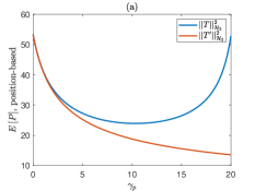
(a)

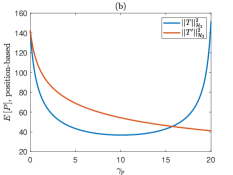
(b)

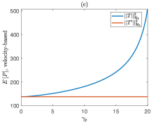
(c)

Figure 4: The expectation of the position-based performance of the double-integrator system (2) given by $\eqref{H_cases_1}$, for $E\left[\Sigma_{0}\right]=I$ and the gains (a) $k_{p}=3,k_{d}=5,\gamma_{d}=0$, (b) $k_{p}=1,k_{d}=2,\gamma_{d}=6.5$. (c) The expectation of the velocity-based performance of the double-integrator system (2) given by $\eqref{H_cases_2}$, for $E\left[\Sigma_{0}\right]=I$ and the gains $k_{p}=1,k_{d}=2,\gamma_{d}=7$.

VI-C Example: Position and Velocity based Performance with Uni-directional vs. Bi-directional Feedback

We now consider a cyclic digraph in which each node has uniform out-degree $d$ and the uniformly weighted edges that start at each node reach $\omega$ succeeding nodes. This results in ‘look-ahead’ type state measurements through $\omega$ communication hops. The respective weighted Laplacian is given by

$$\!\,L^{cyc}(d,\omega)\!=\!d\!\times\!\operatorname{circ}{\left(\begin{bmatrix}1&-\frac{1}{\omega}&\dots&-\frac{1}{\omega}&0&\dots&0\end{bmatrix}\right)}\!,\!\!\!\!\!$$ (68)

where $d\in\mathbb{R}^{+}$, $\omega\in\mathbb{Z}^{+}$, $\omega\leq n-1$ and $\operatorname{circ}(\cdot)$ denotes the circulant matrix generated by permuting the row vector in the argument. The Jordan decomposition of $L=L^{cyc}$ gives [39]

$$J_{k}=\lambda_{k}=d\left(1-\frac{1}{\omega}\sum_{i=1}^{\omega}e^{-\mathbb{j}\frac{2\pi}{n}i(k-1)}\right),$$ (69)

for $k=1,\dots,n$. Choosing $\alpha=\frac{1}{\sqrt{n}}$ in (19), the columns of $\tilde{R}$ are given by

$$\mathbb{r}_{l} =\frac{1}{\sqrt{n}}\begin{bmatrix}1&e^{\mathbb{j}\frac{2\pi}{n}(l-1)}&\dots&e^{\mathbb{j}\frac{2\pi}{n}(l-1)(n-1)}\end{bmatrix}^{*},$$ (70)

for $l=2,\dots,n$. For the special case of uni-directional feedback, we set $d=1$ and $\omega=1$ in (68) therefore

$$L=L^{cyc}(1,1)\quad\text{and}\quad L^{\prime}=\frac{L^{cyc}(1,1)+L^{cyc}(1,1)^{*}}{2},$$

where we have used (57) to also define the corresponding bi-directional feedback. We consider the respective systems $T$ and $T^{\prime}$ with an arbitrary output matrix $C\in\mathbb{R}^{n\times n}$ that satisfies Assumption 2, for $n=50$.

For the double-integrator network (2) given by $\eqref{H_cases_1}$ (position based performance), Figure 4a shows that, as suggested by Item 2) of Theorem 6, using relative position feedback without relative velocity feedback ($\gamma_{p}\neq 0$ and $\gamma_{d}=0$) leads to worse performance with directed interconnection. It is when both relative position and velocity measurements are used ($\gamma_{p}\neq 0$ and $\gamma_{d}\neq 0$) that the directed cycles can be utilized for better performance by tuning the gains. Per Item 3) of Theorem 6, sufficiently small $\gamma_{p}$ (i.e. sufficiently large velocity gains $k_{d}$ and $\gamma_{d}$) improves the performance of the directed interconnection relative to its undirected counterpart; but the performance degrades for sufficiently large $\gamma_{p}$, as shown in Figure 4b. Directed cycles require less communication thus can be preferable, provided the gains are carefully selected.

For the double-integrator network (2) given by $\eqref{H_cases_2}$ (velocity based performance), Figure 4c shows that relative position feedback degrades performance if the cycles are directed. But the performance becomes comparable to that of the undirected system for sufficiently small $\gamma_{p}$, equaling it at $\gamma_{p}=0$. This supports the findings of Theorem 7.

VII All-to-One vs. $\omega$-Nearest Neighbor Networks

In this section, we compare two different relative feedback schemes. The first one is called an all-to-one network, which designates a ‘leader’ node that receives no relative feedback, where the remaining nodes have access to uniformly weighted uni-directional state measurements relative to the leader only. The second one is referred to as an $\omega$-nearest neighbor network, which is based on uniformly weighted uni-directional state measurements of each node relative to $\omega$ succeeding nodes. We consider performance metrics that have circulant output matrices $C$, which arise in many applications such as quantifying lack of coherence in a system in terms of global or local disorder [6, 12, 31].

VII-A Imploding Star Graph: All-to-One Networks

All-to-one networks can be modeled as the imploding star graph whose edge weights are normalized such that the out-degree of each node is $\frac{n}{n-1}$. The corresponding weighted Laplacian is given by

$$L=\frac{n}{n-1}\begin{bmatrix}I_{n-1}&-\mathbb{1}\\ \mathbb{0}^{\intercal}&0\end{bmatrix},$$ (71)

with total out-degree $n$. The Jordan decomposition gives

$$J=\frac{n}{n-1}\begin{bmatrix}0&\mathbb{0}^{\intercal}\\ \mathbb{0}&I_{n-1}\end{bmatrix}.$$ (72)

Choosing $\alpha=1$ in (19), the matrices $\tilde{R}$ and $\tilde{Q}$ are given by

$$\tilde{R}=\begin{bmatrix}I_{n-1}\\ \mathbb{0}^{\intercal}\end{bmatrix}\ \text{and}\ \tilde{Q}=\begin{bmatrix}I_{n-1}&-\mathbb{1}\end{bmatrix}.$$ (73)

VII-A1 Single-Integrator Networks

The next theorem provides the solution for (5) for the single-integrator network (1) using Theorem 3 and the decomposition given by (72) and (73).

Theorem 8.

Consider the single-integrator network (1). Suppose that $\mathcal{G}$ is an imploding star graph with the weighted Laplacian (71), $C$ is circulant and the disturbance has unit covariance, i.e. $E[\Sigma_{0}]=I$. Then the expectation of the performance metric (5) for the system $T$ given by (17) is

$$\!E\left[P\right]\!=\lVert T\rVert_{\mathcal{H}_{2}}^{2}=\,\frac{n-1}{n^{2}}\sum_{i=2}^{n}\, \mu_{i}\Bigg{(}\!n-1\,\,+$$ (74)

$$+ \!\!\!\!\!\!\sum_{\begin{subarray}{c}l>k,\\ k,l\in\{2,\dots,n\}\end{subarray}}\!\!\!\!\!\!\!\!\cos\left(\!\frac{2\pi}{n}(i-1)(l-k)\!\right)\!\!\Bigg{)}\!.\!\!\!$$

Proof.

Using the fact that $E\left[\Sigma_{0}\right]=I$, we have $E\left[P\right]=\operatorname{tr}(\tilde{Q}\tilde{Q}^{*}\Psi)$. (73) leads to $\tilde{Q}\tilde{Q}^{*}=I_{n-1}+\mathbb{1}\mathbb{1}^{\intercal}$ which gives

$$E\left[P\right]=\sum_{k=2}^{n}\Psi_{kk}+\sum_{k=2}^{n}\sum_{l=2}^{n}\Psi_{kl}.$$ (75)

The matrix $M$ in (33) has the eigenvectors

$$\boldsymbol{\theta}_{l}=\frac{1}{\sqrt{n}}\begin{bmatrix}1&e^{\mathbb{j}\frac{2\pi}{n}(l-1)}&\dots&e^{\mathbb{j}\frac{2\pi}{n}(l-1)(n-1)}\end{bmatrix}^{*}$$ (76)

for $l=2,\dots,n$. Using (76) and the columns of $\tilde{R}$ given in (73), the scalar products in (34) are obtained as

$$\left\langle\boldsymbol{\theta}_{i},\mathbb{r}_{k}\right\rangle=\frac{1}{\sqrt{n}}e^{-\mathbb{j}\frac{2\pi}{n}(i-1)(k-2)},\quad k=2,\dots,n.$$ (77)

By (49) and the fact that $\lambda_{i}=\frac{n}{n-1}$ for $i=2,\dots,n$ we have $\Psi_{kl}=\frac{n-1}{2n}\nu_{kl}$, therefore using (34) and (77) results in

$$\small E\left[P\right]=\frac{n-1}{2n^{2}}\!\left(\sum_{k=2}^{n}\sum_{i=2}^{n}\mu_{i}+\sum_{k=2}^{n}\sum_{l=2}^{n}\sum_{i=2}^{n}e^{\mathbb{j}\frac{2\pi}{n}(i-1)(l-k)}\mu_{i}\right)\!\!.\!\!$$ (78)

Rearranging the terms in (78) and using Proposition 1 gives the result. ∎

We now consider a special case of circulant output matrices $C$, which leads to a global measure of disorder that quantifies the aggregate state deviation from the average through

$$C=I-\frac{1}{n}\mathbb{1}\mathbb{1}^{\intercal}=L^{cyc}\left(\frac{n-1}{n},n-1\right).$$ (79)

This metric will be denoted by $P_{dav}$.

Relationship to Previous Results

For $P_{dav}$, the following proposition shows that the result in [5] can be reproduced as a special case of Theorem 8.

Proposition 5.

Consider the single-integrator network (1) and the output matrix (79), i.e. the performance metric $P_{dav}$. Suppose that $\mathcal{G}$ is an imploding star graph with the weighted Laplacian (71), and the disturbance has unit covariance, i.e. $E[\Sigma_{0}]=I$. Then the expectation of the performance metric (5) for the system $T$ given by (17) is

$$E\left[P_{dav}\right]=\lVert T\rVert_{\mathcal{H}_{2}}^{2}=\frac{(n-1)^{2}}{2n}.$$ (80)

Proof.

The fact that $\mu_{i}=1\ \forall i$ and (78) gives

$$E\left[P_{dav}\right]=\frac{n-1}{2n^{2}}\bigg{(}2(n-1)^{2}+\sum_{k\neq l}\sum_{i=2}^{n}e^{\mathbb{j}\frac{2\pi}{n}(i-1)(l-k)}\bigg{)}.$$

Since $\sum_{i=1}^{n}e^{\mathbb{j}\frac{2\pi}{n}(i-1)(l-k)}\!=\!0$ for $l-k\!=\!\pm 1,\dots,\pm(n-2)$,

$$E\left[P_{dav}\right]=\frac{n-1}{2n^{2}}\bigg{(}2(n-1)^{2}-\underbrace{\sum_{k\neq l}e^{\mathbb{j}\frac{2\pi}{n}0(l-k)}}_{=(n-1)(n-2)}\bigg{)}.\quad\mbox{\qed}\!\!\!\!\!\!\!\!\!\!\!\!\!$$

VII-A2 Double-Integrator Networks

Using Corollary 4 from Section V, the following theorem characterizes performance metric (5) for all-to-one networks with double-integrator dynamics (2).

Theorem 9.

Consider the double-integrator network (2). Suppose that $\mathcal{G}$ is an imploding star graph with the weighted Laplacian (71), the output matrix $C$ is circulant and the disturbance has unit covariance, i.e. $E[\Sigma_{0}]=I$. Then the expectation of the performance metric (5) is

$$E\left[P\right]=\lVert T\rVert_{\mathcal{H}_{2}}^{2}=P_{0}\frac{1}{2(k_{p}+\gamma_{p}\frac{n}{n-1})(k_{d}+\gamma_{d}\frac{n}{n-1})}$$ (81)

for the system $T$ given by (17) and

$$E\left[P\right]=\lVert T\rVert_{\mathcal{H}_{2}}^{2}=P_{0}\frac{1}{2(k_{d}+\gamma_{d}\frac{n}{n-1})}$$ (82)

for the system $T$ given by (18), where

$$P_{0}=\frac{1}{n}\left(\sum_{k=2}^{n}\sum_{i=2}^{n}\mu_{i}+\sum_{k=2}^{n}\sum_{l=2}^{n}\sum_{i=2}^{n}e^{\mathbb{j}\frac{2\pi}{n}(i-1)(l-k)}\mu_{i}\right).$$

Furthermore, if the output matrix is given by (79), then

$$E\left[P_{dav}\right]=\lVert T\rVert_{\mathcal{H}_{2}}^{2}=\frac{n-1}{2(k_{p}+\gamma_{p}\frac{n}{n-1})(k_{d}+\gamma_{d}\frac{n}{n-1})}$$ (83)

for the system $T$ given by (17) and

$$E\left[P_{dav}\right]=\lVert T\rVert_{\mathcal{H}_{2}}^{2}=\frac{n-1}{2(k_{d}+\gamma_{d}\frac{n}{n-1})}$$ (84)

for the system $T$ given by (18).

Proof.

Substitution of $\lambda_{k}=\frac{n}{n-1}$ for $k=2,\dots,n$ into (53) and (54) gives $\Psi_{kl}=\nu_{kl}\frac{1}{2(k_{p}+\gamma_{p}\frac{n}{n-1})(k_{d}+\gamma_{d}\frac{n}{n-1})}$ for the system $T$ given by (17) and $\Psi_{kl}=\nu_{kl}\frac{1}{2(k_{d}+\gamma_{d}\frac{n}{n-1})}$ for the system $T$ given by (18). By the argument given in the proof of Theorem 8, using the expressions above and (75) leads to (81) and (82). The argument given in the proof of Proposition 5 combined with (81) and (82) yields (83) and (84). ∎

When $P_{dav}$ is considered, Proposition 5 and Theorem 9 show that the performance metric grows unboundedly with the network size. Next we study $\omega$-nearest neighbor networks.

VII-B Cyclic Digraphs: $\omega$-Nearest Neighbor Networks

The cyclic digraph defined by the weighted Laplacian (68) can be used to model $\omega$-nearest neighbor networks. In order to normalize the edge weights of the digraphs with different number of communication hops we choose the out-degree of each node as $d=1$ in (68), which leads to

$$L=L^{cyc}\left(1,\omega\right)$$ (85)

so that the total out-degree in the graph is $n$. Since we consider circulant output matrices $C$, the eigenvectors of $M$ in (33) are given by (76). Combining this with (70), the scalar products in (34) are obtained as

$$\left\langle\boldsymbol{\theta}_{l},\mathbb{r}_{k}\right\rangle=\begin{cases}1&k=l\\ 0&k\neq l\end{cases},\ k=2,\dots,n,$$ (86)

therefore (34) leads to

$$\nu_{kk}=\mu_{k}.$$ (87)

This means that the dependence of (50), (55) and (56) on the output matrix $C$ is only through the eigenvalues $\mu_{k}$ of $M$.

Then performance is given by (50) for the single-integrator system, and by (55) or (56) for the double-integrator system, where due to (69) the eigenvalues of $L$ satisfy

$$\lambda_{k}=1-\frac{1}{\omega}\sum_{i=1}^{\omega}e^{-\mathbb{j}\frac{2\pi}{n}i(k-1)},\ k=1,\dots,n.$$ (88)

Next we present two examples to demonstrate the effect of the number of communication hops $\omega$ on the performance of $\omega$-nearest neighbor networks and to investigate the relationship between all-to-one and all-to-all communication structures.

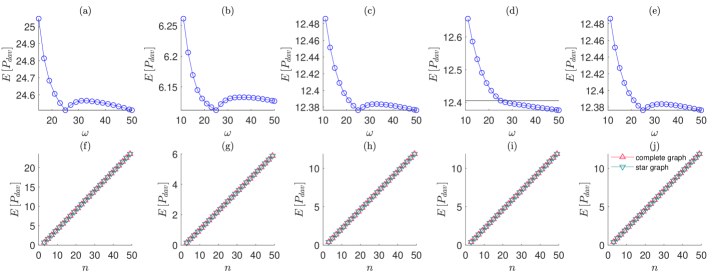
Figure 5: (Top) The expectation of $P_{dav}$ defined by (79) versus the number of communication hops $\omega$ of the $\omega$-nearest neighbor networks given by (85) where the network size is $n=51$. (Bottom) The expectation of $P_{dav}$ versus the network size $n$ for the imploding star graph and the complete graph given by (71) and (89). The disturbance has unit covariance, i.e. $E[\Sigma_{0}]=I$. Plots respectively illustrate the cases of: (a, f) single-integrator (1) given by $\eqref{H_cases_1}$, (b, g) double-integrator (2) given by $\eqref{H_cases_1}$ (position-based performance), $k_{p}=k_{d}=\gamma_{p}=\gamma_{d}=1$, (c, h) double-integrator (2) given by $\eqref{H_cases_1}$ (position-based performance), $k_{p}=k_{d}=\gamma_{d}=1,\gamma_{p}=0$, (d, i) double-integrator (2) given by $\eqref{H_cases_2}$ (velocity-based performance), $k_{p}=k_{d}=\gamma_{p}=\gamma_{d}=1$, (e, j) double-integrator (2) given by $\eqref{H_cases_2}$ (velocity-based performance), $k_{p}=k_{d}=\gamma_{d}=1,\gamma_{p}=0$.

VII-C Example: Number of Communication Hops

In the following we investigate how performance changes with respect to $\omega$. We first show that performance does not necessarily improve by increasing $\omega$, i.e. through communication with a larger number of nearest neighbors.

For convenience suppose that $n$ is odd. Consider the case where $\omega=\frac{n-1}{2}$ such that $L=L^{cyc}(1,\frac{n-1}{2})$. Using the definition given by (57)

$$L^{\prime}=\frac{L^{cyc}(1,\frac{n-1}{2})+L^{cyc}(1,\frac{n-1}{2})^{*}}{2}=L^{cyc}(1,n-1),$$ (89)

i.e. $L^{\prime}$ is the weighted Laplacian associated with the complete graph with uniform edge weights $\frac{1}{n-1}$. Then the associated systems $T$ and $T^{\prime}$ have the following properties for any performance metric satisfying Assumption 2:

• $\lVert T\rVert_{\mathcal{H}_{2}}^{2}=\lVert T^{\prime}\rVert_{\mathcal{H}_{2}}^{2}$ for the single-integrator network (1) defined by $\eqref{H_cases_1}$ due to Theorem 5,

• It is possible due to Theorem 6 that $\lVert T\rVert_{\mathcal{H}_{2}}^{2}<\lVert T^{\prime}\rVert_{\mathcal{H}_{2}}^{2}$, $\lVert T\rVert_{\mathcal{H}_{2}}^{2}=\lVert T^{\prime}\rVert_{\mathcal{H}_{2}}^{2}$ or $\lVert T\rVert_{\mathcal{H}_{2}}^{2}>\lVert T^{\prime}\rVert_{\mathcal{H}_{2}}^{2}$ for the position based performance of the double-integrator network (2) defined by system (17),

• It can only hold that $\lVert T\rVert_{\mathcal{H}_{2}}^{2}=\lVert T^{\prime}\rVert_{\mathcal{H}_{2}}^{2}$ or $\lVert T\rVert_{\mathcal{H}_{2}}^{2}>\lVert T^{\prime}\rVert_{\mathcal{H}_{2}}^{2}$ for the velocity based performance of the double-integrator network (2) defined by system (18) due to Theorem 7.

As this example suggests, using half the number of communication hops as compared to the complete graph, i.e. the case in which $\omega$ is maximal, provides identical performance for the single integrator network (1). It is possible to achieve better performance using half the number of hops compared to the complete graph in the case of the position based metrics of the double integrator network (2); but this is not the case for the velocity based metrics.

The dependence of $E\left[P_{dav}\right]$ on $\omega$ is illustrated in figures 5a - 5e for a case in which $n=51$ and the disturbance has unit covariance, i.e. $E[\Sigma_{0}]=I$. For the single integrator network (1) we observe in Figure 5a that $\lVert T\rVert_{\mathcal{H}_{2}}^{2}=\lVert T^{\prime}\rVert_{\mathcal{H}_{2}}^{2}$. This is also true for the position and velocity based performance of the double-integrator network (2) if relative position feedback is absent ($k_{p}=k_{d}=\gamma_{d}=1$ and $\gamma_{p}=0$) as shown in figures 5c (due to Item 1 in Theorem 6) and 5e (due to Item 3 in Theorem 7). Conversely, using relative position feedback ($k_{p}=k_{d}=\gamma_{p}=\gamma_{d}=1$) leads to $\lVert T\rVert_{\mathcal{H}_{2}}^{2}<\lVert T^{\prime}\rVert_{\mathcal{H}_{2}}^{2}$ as shown in Figure 5b (due to Item 3 in Theorem 6) for the position based performance and to $\lVert T\rVert_{\mathcal{H}_{2}}^{2}>\lVert T^{\prime}\rVert_{\mathcal{H}_{2}}^{2}$ as shown in Figure 5d (due to Item 2 in Theorem 7) for the velocity based performance. For all cases, increasing $\omega$ up to $\omega=25$ monotonically improves performance. Compared to $\omega=25$, choosing $25<\omega<50$ degrades performance, excluding the velocity based performance with relative position feedback ($\gamma_{p}\neq 0$, Figure 5d) which improves monotonically as $\omega$ is increased. Therefore at least for $n=51$ and the cases in figures 5a-5c and 5e, $\omega=\frac{n-1}{2}$ provides the optimal performance.

The next example provides a comparison between all-to-one and all-to-all networks.

VII-D Example: All-to-One versus All-to-All Networks

For the special case of $P_{dav}$ which is determined by (79), (87) holds and we have $\mu_{k}=1$ for $k=2,\dots,n$. If all-to-all networks are considered, i.e. $L$ is given by (89), (88) reduces to $\lambda_{k}=\frac{n}{n-1}$ for $k=2,\dots,n$. Then $P_{dav}$ is given by

• (80) for the single-integrator network (1) given by (17),

• (83) for the double-integrator network (2) given by (17),

• (84) for the double-integrator network (2) given by (18),

where we respectively used (50), (59) and (63). Therefore, $\omega$-nearest neighbor networks with $\omega=n-1$ (all-to-all) and all-to-one networks perform identically if $P_{dav}$ is considered, which is illustrated in figures 5f - 5j for up to $n=49$. In conclusion, given that the total out-degree is normalized to be $n$ for each graph, the same $P_{dav}$ is achieved by using $n-1$ directed edges that follow a common leader as that of using $n(n-1)$ directed edges such that each node follows every other node. The latter feedback scheme can be interpreted as every node being a common leader in the sense of the former feedback scheme. In other words, the all-to-all network can be interpreted as the superposition of $n$ all-to-one networks with edge weights scaled by $\frac{1}{n}$. Thus the same level of deviation from the average state (position or velocity) is achieved by following a single common leader instead of using all-to-all communication, provided the edge weights are sufficiently large. As $n$ grows, the number of edges grow linearly and each edge weight $\frac{n}{n-1}$ remains bounded in all-to-one networks. In contrast, the number of edges grow quadratically and each edge weight $\frac{1}{n-1}$ decays to zero in all-to-all networks. We note for double-integrator networks (2) given by (17) that compared to both all-to-one and all-to-all communication, it is possible to achieve better position-based $P_{dav}$ with $\omega=\frac{n-1}{2}$ nearest neighbor interactions (odd $n$), if both relative position and velocity feedback are employed and the relative position feedback gain $\gamma_{p}$ is sufficiently small (e.g. Figure 5b).

VIII Conclusions

We studied the performance of single and double integrator networks over arbitrary digraphs that have at least one globally reachable node. Using a unifying framework, closed-form solutions are provided for a general class of output $\mathcal{L}_{2}$ norm based quadratic performance metrics. The special case of normal weighted Laplacian matrices reveals the importance of judicious control design for mitigating any performance degradation in directed networks, and possibly improving upon their undirected counterparts. In addition, we have demonstrated that performance is sensitive to the degree of connectivity (e.g. range of communication in $\omega$-nearest neighbor networks), but it does not depend on it monotonically. This non-monotonicity can also be deduced from the equivalence between all-to-one and all-to-all networks. That is, the same level of state deviation from the average is achieved using either network architecture.

-A Lemmas from Subsection IV-B

Lemma 6.

Consider the transfer function

$$\Omega_{k,\delta}(s)=\frac{r(s){\left(\gamma_{p}+s\gamma_{d}\right)}^{\delta-1}}{{\left[s^{2}+(k_{d}+\gamma_{d}\lambda_{k})s+k_{p}+\gamma_{p}\lambda_{k}\right]}^{\delta}}$$ (90)

for some $\delta\in\mathbb{Z}_{+}$. Suppose that $s^{2}+(k_{d}+\gamma_{d}\lambda_{k})s+k_{p}+\gamma_{p}\lambda_{k}=0$ has distinct roots $\rho_{1}^{(k)}$ and $\rho_{2}^{(k)}$, i.e. $\rho_{1}^{(k)}\neq\rho_{2}^{(k)}$. Then, $\Omega_{k,\delta}(s)$ has a realization $\left(\mathcal{A}_{k,\delta},\mathcal{B}_{k,\delta},\mathcal{C}_{k,\delta}\right)$ in Jordan canonical form given by

$$\mathcal{A}_{k,\delta}=\operatorname{blockdiag}{\left(\mathcal{J}(\rho_{i}^{(k)},\delta)\right)_{i=1,2}},$$ (91)

$\mathcal{B}_{k,\delta}=\bigg{[}\underbrace{\begin{matrix}0&\dots&1\end{matrix}}_{1\times\delta}\underbrace{\begin{matrix}0&\dots&1\end{matrix}}_{1\times\delta}\bigg{]}^{\intercal}$, $\mathcal{C}_{k,\delta}=\begin{bmatrix}c_{1}^{(k)}&\dots&c_{2\delta}^{(k)}\end{bmatrix}$, where $\mathcal{J}(\rho_{1}^{(k)},\delta)$ denotes the size-$\delta$ Jordan block with the eigenvalue $\rho_{1}^{(k)}$.

If $r(s)=1$, i.e. we consider system $T$ given by (17), the elements of $\mathcal{C}_{k,\delta}$ are given by

$$c_{l}^{(k)} =\sum_{\zeta=0}^{l-1}\tau(\zeta,l){\gamma_{d}}^{\zeta}\frac{{(\gamma_{p}+\rho_{1}^{(k)}\gamma_{d})}^{\delta-\zeta-1}}{{(\rho_{1}^{(k)}-\rho_{2}^{(k)})}^{\delta+l-\zeta-1}},$$

$$c_{l+\delta}^{(k)} =\sum_{\zeta=0}^{l-1}\tau(\zeta,l){\gamma_{d}}^{\zeta}\frac{{(\gamma_{p}+\rho_{2}^{(k)}\gamma_{d})}^{\delta-\zeta-1}}{{(\rho_{2}^{(k)}-\rho_{1}^{(k)})}^{\delta+l-\zeta-1}},$$

if $r(s)=s$, i.e. we consider system $T$ given by (18), the elements of $\mathcal{C}_{k,\delta}$ are given by

$$c_{l}^{(k)} =\sum_{\zeta=0}^{l-1}\tau(\zeta,l){\gamma_{d}}^{\zeta-1}\left(\frac{\zeta\gamma_{p}+\delta\rho_{1}^{(k)}\gamma_{d}}{\delta-\zeta}\right)\frac{{(\gamma_{p}+\rho_{1}^{(k)}\gamma_{d})}^{\delta-\zeta-1}}{{(\rho_{1}^{(k)}-\rho_{2}^{(k)})}^{\delta+l-\zeta-1}},$$

$$c_{l+\delta}^{(k)} =\sum_{\zeta=0}^{l-1}\tau(\zeta,l){\gamma_{d}}^{\zeta-1}\left(\frac{\zeta\gamma_{p}+\delta\rho_{2}^{(k)}\gamma_{d}}{\delta-\zeta}\right)\frac{{(\gamma_{p}+\rho_{2}^{(k)}\gamma_{d})}^{\delta-\zeta-1}}{{(\rho_{2}^{(k)}-\rho_{1}^{(k)})}^{\delta+l-\zeta-1}},$$

for $l=1,\dots,\delta$, where $\tau(\zeta,l)={(-1)}^{l-\zeta-1}\binom{l-1}{\zeta}\binom{\delta+l-\zeta-2}{l-1}$.

Proof.

Using the fact that the denominator of $\Omega_{k,\delta}(s)$ has distinct roots

$$\Omega_{k,\delta}(s)=\frac{\Gamma(s)}{{(s-\rho_{1}^{(k)})}^{\delta}{(s-\rho_{2}^{(k)})}^{\delta}},$$

where $\Gamma(s)=r(s){\left(\gamma_{p}+s\gamma_{d}\right)}^{\delta-1}$. Applying partial fractions, we have

$$\Omega_{k,\delta}(s)=\sum_{l=1}^{\delta}\frac{c_{l}^{(k)}}{{(s-\rho_{1}^{(k)})}^{\delta-l+1}}+\frac{c_{l+\delta}^{(k)}}{{(s-\rho_{2}^{(k)})}^{\delta-l+1}},$$ (92)

which can be represented by the Jordan canonical realization (91). Here the coefficients $c_{l}^{(k)}$ and $c_{l+\delta}^{(k)}$ are given by

$$c_{l}^{(k)} =\frac{1}{(l-1)!}\lim_{s\to\rho_{1}^{(k)}}\frac{d^{l-1}}{ds^{l-1}}\left[{(s-\rho_{1}^{(k)})}^{\delta}\Omega_{k,\delta}(s)\right],$$ (93)

$$c_{l+\delta}^{(k)} =\frac{1}{(l-1)!}\lim_{s\to\rho_{2}^{(k)}}\frac{d^{l-1}}{ds^{l-1}}\left[{(s-\rho_{2}^{(k)})}^{\delta}\Omega_{k,\delta}(s)\right].$$ (94)

The general Leibniz rule for the derivative of product yields

$$\!\!\!\!\!\!c_{l}^{(k)}\! =\!\!\lim_{s\to\rho_{1}^{(k)}}\!\sum_{\zeta=0}^{l-1}\frac{\binom{l-1}{\zeta}}{(l-1)!}\frac{d^{\zeta}\Gamma(s)}{ds^{\zeta}}\frac{d^{l-1-\zeta}}{ds^{l-1-\zeta}}\!\!\left[{(s-\rho_{2}^{(k)})}^{-\delta}\right]\!\!,\!\!$$ (95)

$$\!\!\!\!c_{l+\delta}^{(k)}\! =\!\!\lim_{s\to\rho_{2}^{(k)}}\!\sum_{\zeta=0}^{l-1}\frac{\binom{l-1}{\zeta}}{(l-1)!}\frac{d^{\zeta}}{ds^{\zeta}}\Gamma(s)\frac{d^{l-1-\zeta}}{ds^{l-1-\zeta}}\left[{(s-\rho_{1}^{(k)})}^{-\delta}\right]\!\!,\!$$ (96)

For the cases of $r(s)=1$ or $r(s)=s$, a direct calculation shows that

$$\!\frac{d^{\zeta}}{ds^{\zeta}}\left[{(\gamma_{p}+s\gamma_{d})}^{\delta-1}\right]\!\!=\!{\gamma_{d}}^{\zeta}\frac{(\delta-1)!}{(\delta-\zeta-1)!}{(\gamma_{p}+s\gamma_{d})}^{\delta-\zeta-1}\!,\!\!\!\!$$ (97)

$$\!\!\!\!\!\!\!\!\!\!\frac{d^{\zeta}}{ds^{\zeta}}\left[{s(\gamma_{p}+s\gamma_{d})}^{\delta-1}\right]\!\! =\!s{\gamma_{d}}^{\zeta}\frac{(\delta-1)!}{(\delta-\zeta-1)!}{(\gamma_{p}+s\gamma_{d})}^{\delta-\zeta-1}$$

$$+{\gamma_{d}}^{\zeta-1}\zeta\frac{(\delta-1)!}{(\delta-\zeta)!}{(\gamma_{p}+s\gamma_{d})}^{\delta-\zeta}\!,\!\!$$ (98)

$$\frac{d^{l-1-\zeta}}{ds^{l-1-\zeta}}\left[{(s-\rho_{2}^{(k)})}^{-\delta}\right]={(-1)}^{l-1-\zeta}\frac{(\delta+l-\zeta-2)!}{(\delta-1)!}{(s-\rho_{2}^{(k)})}^{-\delta-l+\zeta+1}.$$ (99)

Substituting (97), (98) and (99) into (95) and taking the limit gives the desired result. A similar procedure can be followed to evaluate the expression in (96). ∎

Lemma 7.

Consider the transfer function $\Omega_{k,\delta}(s)$ in (90) for some $\delta\in\mathbb{Z}_{+}$. Suppose that $s^{2}+(k_{d}+\gamma_{d}\lambda_{k})s+k_{p}+\gamma_{p}\lambda_{k}=0$ has repeated roots $\rho_{1}^{(k)}$ and $\rho_{2}^{(k)}$, i.e. $\rho_{1}^{(k)}=\rho_{2}^{(k)}=\rho^{(k)}$. Then, $\Omega_{k,\delta}(s)$ has a realization $\left(\mathcal{A}_{k,\delta},\mathcal{B}_{k,\delta},\mathcal{C}_{k,\delta}\right)$ in Jordan canonical form given by

$$\mathcal{A}_{k,\delta}=\mathcal{J}(\rho^{(k)},2\delta),$$ (100)

$$\mathcal{B}_{k,\delta}=\bigg{[}\underbrace{\begin{matrix}0&\dots&1\end{matrix}}_{1\times 2\delta}\bigg{]}^{\intercal},\mathcal{C}_{k,\delta}=\begin{bmatrix}c_{1}^{(k)}&\dots&c_{2\delta}^{(k)}\end{bmatrix}.$$

If $r(s)=1$, i.e. we consider system $T$ given by (17), the elements of $\mathcal{C}_{k,\delta}$ are given by

$$c_{l}^{(k)}=\begin{cases}{\gamma_{d}}^{l-1}\binom{\delta-1}{l-1}{(\gamma_{p}+\rho^{(k)}\gamma_{d})}^{\delta-l},&1\leq l\leq\delta\\ \hfil 0,&\delta+1\leq l\leq 2\delta\end{cases},$$

if $r(s)=s$, i.e. we consider system $T$ given by (18), the elements of $\mathcal{C}_{k,\delta}$ are given by

$$c_{l}^{(k)}\!=\!\begin{cases}\!\left[\frac{(l-1)\gamma_{p}+\delta\rho^{(k)}\gamma_{d}}{\delta-l+1}\right]\!{\gamma_{d}}^{l-2}\binom{\delta-1}{l-1}{(\gamma_{p}+\rho^{(k)}\gamma_{d})}^{\delta-l},&1\leq l\leq\delta\\ \hfil{\gamma_{d}}^{\delta-1},&l=\delta+1\\ \hfil 0,&\delta+2\leq l\leq 2\delta\end{cases}.$$

Proof.

Using the fact that $\Omega_{k,\delta}(s)$ has repeated roots leads to

$$\Omega_{k,\delta}(s)=\frac{r(s){\left(\gamma_{p}+s\gamma_{d}\right)}^{\delta-1}}{{(s-\rho^{(k)})}^{2\delta}}.$$

Applying partial fractions, we have

$$\Omega_{k,\delta}(s)=\sum_{l=1}^{2\delta}\frac{c_{l}^{(k)}}{{(s-\rho^{(k)})}^{2\delta-l+1}},$$

which can be represented by the Jordan canonical realization (100). Here the coefficients $c_{l}^{(k)}$ are given by

$$c_{l}^{(k)}=\frac{1}{(l-1)!}\lim_{s\to\rho^{(k)}}\frac{d^{l-1}}{ds^{l-1}}\left[r(s){\left(\gamma_{p}+s\gamma_{d}\right)}^{\delta-1}\right].$$ (101)

For the cases of $r(s)=1$ or $r(s)=s$, using respectively (97) and (98) and taking the limit in (101) gives the desired result. ∎

References

- [1] W. Ren and E. Atkins, “Second-order consensus protocols in multiple vehicle systems with local interactions,” in AIAA Guidance, Navigation, and Control Conf. and Exhibit, Aug. 2005, pp. 6238–6251.
- [2] W. Yu, G. Chen, and M. Cao, “Some necessary and sufficient conditions for second-order consensus in multi-agent dynamical systems,” Automatica, vol. 46, no. 9, pp. 1089–1095, Jun. 2010.
- [3] J. Zhu, Y. Tian, and J. Kuang, “On the general consensus protocol of multi-agent systems with double-integrator dynamics,” Linear Algebra Appl., vol. 431, no. 5-7, pp. 701–715, Aug. 2009.
- [4] M. Siami and N. Motee, “Fundamental limits and tradeoffs on disturbance propagation in linear dynamical networks,” IEEE Trans. Autom. Control, vol. 61, no. 12, pp. 4055–4062, Dec. 2016.
- [5] G. F. Young, L. Scardovi, and N. E. Leonard, “Robustness of noisy consensus dynamics with directed communication,” in Proc. of the American Ctrl. Conf., Jun. 2010, pp. 6312–6317.
- [6] B. Bamieh, M. R. Jovanović, P. Mitra, and S. Patterson, “Coherence in large-scale networks: Dimension-dependent limitations of local feedback,” IEEE Trans. Autom. Control, vol. 57, no. 9, pp. 2235–2249, Sep. 2012.
- [7] S. Dezfulian, Y. Ghaedsharaf, and N. Motee, “On performance of time-delay linear consensus networks with directed interconnection topologies,” in Proc. of the American Ctrl. Conf., Jun. 2018.
- [8] T. Sarkar, M. Roozbehani, and M. A. Dahleh, “Asymptotic robustness in consensus networks,” in 2018 Annual American Control Conference (ACC), June 2018, pp. 6212–6217.
- [9] X. Ma and N. Elia, “Mean square performance and robust yet fragile nature of torus networked average consensus,” IEEE Trans. on Ctrl. of Network Systems, vol. 2, no. 3, pp. 216–225, Sep. 2015.
- [10] F. Lin, M. Fardad, and M. R. Jovanović, “Performance of leader-follower networks in directed trees and lattices,” in in Proc. of the 51st IEEE Conf. on Dec. and Ctrl., Dec. 2012, pp. 734–739.
- [11] T. W. Grunberg and D. F. Gayme, “Performance measures for linear oscillator networks over arbitrary graphs,” IEEE Trans. on Ctrl. of Network Systems, vol. 5, no. 1, pp. 456–468, Mar. 2018.
- [12] E. Tegling, P. Mitra, H. Sandberg, and B. Bamieh, “On fundamental limitations of dynamic feedback control in regular large-scale networks,” IEEE Transactions on Automatic Control, Apr. 2019, doi: 10.1109/TAC.2019.2909811.
- [13] R. Pates, C. Lidström, and A. Rantzer, “Control using local distance measurements cannot prevent incoherence in platoons,” in In Proc. of the 56th IEEE Conf. on Dec. and Ctrl., Dec. 2017, pp. 3461–3466.
- [14] H. Hao and P. Barooah, “Stability and robustness of large platoons of vehicles with double-integrator models and nearest neighbor interaction,” International Journal of Robust and Nonlinear Control, vol. 23, no. 18, pp. 2097–2122, Dec. 2013.
- [15] F. Lin, M. Fardad, and M. R. Jovanović, “Optimal control of vehicular formations with nearest neighbor interactions,” IEEE Trans. Autom. Control, vol. 57, no. 9, pp. 2203–2218, Sep. 2012.
- [16] H. G. Oral, E. Mallada, and D. F. Gayme, “Performance of first and second order linear networked systems over digraphs,” in Proc. of the 56th IEEE Conf. on Dec. and Ctrl., Dec. 2017, pp. 1688–1694.
- [17] B. Bamieh and D. F. Gayme, “The price of synchrony: Resistive losses due to phase synchronization in power networks,” in Proc. of the American Ctrl. Conf., Jun. 2013, pp. 5815–5820.
- [18] E. Tegling, B. Bamieh, and D. F. Gayme, “The price of synchrony: Evaluating the resistive losses in synchronizing power networks,” IEEE Transactions on Control of Network Systems, vol. 2, no. 3, pp. 254–266, Sep. 2015.
- [19] E. Tegling, D. F. Gayme, and H. Sandberg, “Performance metrics for droop-controlled microgrids with variable voltage dynamics,” in Proc. of the 54th IEEE Conf. on Dec. and Ctrl., Dec. 2015, pp. 7502–7509.
- [20] E. Mallada, “iDroop: A dynamic droop controller to decouple power grid’s steady-state and dynamic performance,” in 55th IEEE Conference on Decision and Control (CDC), Dec. 2016, pp. 4957–4964.
- [21] Y. Jiang, R. Pates, and E. Mallada, “Performance tradeoffs of dynamically controlled grid-connected inverters in low inertia power systems,” in 56th IEEE Conference on Decision and Control (CDC), Dec. 2017, pp. 5098–5105.
- [22] E. Weitenberg, Y. Jiang, C. Zhao, E. Mallada, C. De Persis, and F. Dorfler, “Robust decentralized secondary frequency control in power systems: Merits and trade-offs,” IEEE Transactions on Automatic Control, Dec. 2018, doi: 10.1109/TAC.2018.2884650.
- [23] X. Wu, F. Dörfler, and M. R. Jovanović, “Input-output analysis and decentralized optimal control of inter-area oscillations in power systems,” IEEE Transactions on Power Systems, vol. 31, no. 3, pp. 2434–2444, May 2016.
- [24] J. W. Simpson-Porco, B. K. Poolla, N. Monshizadeh, and F. Dörfler, “Quadratic performance of primal-dual methods with application to secondary frequency control of power systems,” in 2016 IEEE 55th Conference on Decision and Control (CDC), Dec 2016, pp. 1840–1845.
- [25] H. G. Oral and D. F. Gayme, “Performance of droop-controlled microgrids with heterogeneous inverter ratings,” in Proc. of the European Ctrl. Conf., Jun. 2019, pp. 1398–1405.
- [26] M. Tyloo and P. Jacquod, “Global robustness versus local vulnerabilities in complex synchronous networks,” Phys. Rev. E, vol. 100, p. 032303, Sep. 2019.
- [27] S. Patterson, Y. Yi, and Z. Zhang, “A resistance-distance-based approach for optimal leader selection in noisy consensus networks,” IEEE Transactions on Control of Network Systems, vol. 6, no. 1, pp. 191–201, March 2019.
- [28] W. Ellens, F. M. Spieksma, P. V. Mieghem, A. Jamakovic, and R. E. Kooij, “Effective graph resistance,” Linear Algebra Appl., vol. 435, no. 10, pp. 2491–2506, Nov. 2011.
- [29] G. F. Young, L. Scardovi, and N. E. Leonard, “A new notion of effective resistance for directed graphs– part i: Definition and properties,” IEEE Trans. Autom. Control, vol. 61, no. 7, pp. 1727–1736, Jul. 2016.
- [30] ——, “A new notion of effective resistance for directed graphs– part ii: Computing resistances,” IEEE Trans. Autom. Control, vol. 61, no. 7, pp. 1737–1752, Jul. 2016.
- [31] H. G. Oral and D. F. Gayme, “Disorder in large-scale networks with uni-directional feedback,” in Proc. of the American Ctrl. Conf., Jul. 2019, pp. 3394–3401.
- [32] M. Siami and N. Motee, “New spectral bounds on h2-norm of linear dynamical networks,” Automatica, vol. 80, pp. 305–312, Jun. 2017.
- [33] F. Paganini and E. Mallada, “Global performance metrics for synchronization of heterogeneously rated power systems: The role of machine models and inertia,” in 2017 55th Annual Allerton Conference on Communication, Control, and Computing (Allerton), Oct 2017, pp. 324–331.
- [34] ——, “Global analysis of synchronization performance for power systems: bridging the theory-practice gap,” arXiv preprint, May 2019, arXiv:1905.06948.
- [35] T. Coletta and P. Jacquod, “Performance measures in electric power networks under line contingencies,” IEEE Transactions on Control of Network Systems, Apr. 2019, doi: 10.1109/TCNS.2019.2913554.
- [36] C. Ji, E. Mallada, and D. F. Gayme, “Evaluating robustness of consensus algorithms under measurement error over digraphs,” in 2018 IEEE Conference on Decision and Control (CDC), Dec 2018, pp. 1238–1244.
- [37] F. Bullo, “Lectures on network systems,” Online at http://motion.me.ucsb.edu/book-lns, with contributions by J. Cortes, F. Dorfler and S. Martinez, 2016.
- [38] Z. Li, Z. Duan, G. Chen, and L. Huang, “Consensus of multiagent systems and synchronization of complex networks: A unified viewpoint,” IEEE Trans. Circuits Syst. I, vol. 57, no. 1, pp. 213–224, Jan. 2010.
- [39] R. Horn and C. R. Johnson, Matrix Analysis. Cambridge University Press, 1985.