Dirac integral equations for dielectric and plasmonic scattering

Abstract.

A new integral equation formulation is presented for the Maxwell transmission problem in Lipschitz domains. It builds on the Cauchy integral for the Dirac equation, is free from false eigenwavenumbers for a wider range of permittivities than other known formulations, can be used for magnetic materials, is applicable in both two and three dimensions, and does not suffer from any low-frequency breakdown. Numerical results for the two-dimensional version of the formulation, including examples featuring surface plasmon waves, demonstrate competitiveness relative to state-of-the-art integral formulations that are constrained to two dimensions. However, our Dirac integral equation performs equally well in three dimensions, as demonstrated in a companion paper.

1. Introduction

This paper introduces a new boundary integral equation (BIE) formulation for solving the time-harmonic Maxwell transmission problem across interfaces between domains of constant and isotropic, but otherwise general complex-valued, permittivities and permeabilities. The main novelty of our BIE is that it performs well for a very wide range of materials, including metamaterials with negative permittivities. We provide not only numerical evidence of such performance, but also rigorous proofs for general Lipschitz interfaces.

We refer to our new formulation as a Dirac integral equation, since our point of departure is to embed Maxwell’s equations into a Dirac-type equation by relaxing the constraints ${\text{{\rm div}}}E=0$ and ${\text{{\rm div}}}B=0$ on the electric and magnetic fields $E$ and $B$ and introducing two auxiliary Dirac variables, which make the partial differential equation (PDE) elliptic also without these divergence-free constraints. This means that our integral equation uses eight unknown scalar densities in three dimensions (3D) and four unknown scalar densities in two dimensions (2D), where eight and four, respectively, are the dimensions of the Clifford algebra which is the algebraic structure behind the Dirac equation and which we make use of in the analysis. This idea to write Maxwell’s equations as a Dirac equation is old, and appears in the works of M. Riesz and D. Hestenes. Even Maxwell himself formulated his equations using Hamilton’s quaternions. Picard [33, 34] elliptifies Maxwell’s equations by embedding these into a Dirac equation, without using Clifford algebra but writing it as a div-curl-grad matrix system. This Picard’s extended Maxwell system is the basis for more recent works [40, 39, 38].

In harmonic analysis of non-smooth boundary value problems for Maxwell’s equations, BIEs based on the Dirac equation were developed by M. Mitrea, McIntosh et al., see [31, 5]. Building on this, the second author of the present paper further developed the theory of Dirac integral equations for solving Maxwell’s equations in his PhD work [2, 3, 1, 6, 4] with Alan McIntosh. Applications of these methods to scattering from perfect electric conductors (PEC) are found in [35, 36], and the spin integral equations there are precursors of the Dirac integral equations presented here. More recent results on Dirac equations for Maxwell scattering problems with Lipschitz interfaces are also [30, 26], which deal with the $L_{p}$ boundary topology, but only treat the case of equal wave numbers in the two domains.

The focus in the present paper is on BIEs which are numerically good for a very wide range of material combinations, including such where permittivity ratios are negative real numbers. In this case, the relevant function space is the trace space for the $L_{2}$ topology in the domains, since this is where surface plasmons waves may appear, as we approach purely negative permittivity ratios. In particular, we seek BIEs without false eigenwavenumbers in this plasmonic regime. In the simpler cases of scattering from PEC objects or from dielectric objects with less permissible restrictions on their permittivities, and also on the genus of the domains, there are many good formulations available. See, for example, [15] for a BIE with six scalar unknowns containing only weakly singular integral operators and extending results from the pioneering work [40]. However, for metamaterials in plasmonic scattering, we are only aware of two BIEs without false eigenwavenumbers, namely the Dirac integral equations presented here and the BIE in [23]. Both these works seem to indicate that eight is the number of scalar densities needed to construct a Maxwell BIE in 3D that is free from false eigenwavenumbers for all complex-valued choices of material constants.

Turning to the description of the present work, the main objective is to design the integral equations so that not only the operator has good Fredholm properties, but also so that no false eigenwavenumbers appear. This problem may be best explained by the relation

$$\text{PDE}\circ\text{Ansatz}=\text{BIE}\,.$$

The PDE problem, Helmholtz or Maxwell, is to invert a map $(F^{+},F^{-})\mapsto g$, where $g$ is boundary datum, and $F^{\pm}$ are the solutions, the sought fields in the interior domain $\Omega^{+}$ and exterior domain $\Omega^{-}$, respectively. To obtain a BIE we need to choose an appropriate ansatz, that is an integral representation $h\mapsto(F^{+},F^{-})$ of the fields in terms of a density function $h$ on the interface $\partial\Omega$ between $\Omega^{+}$ and $\Omega^{-}$. From this we obtain a BIE as the composed map $h\mapsto g$, via $(F^{+},F^{-})$. A main objective is to use an invertible ansatz with as good condition number as possible, so that the BIE is invertible whenever the PDE problem is well posed.

Our main results, the Dirac integral equations for solving Maxwell’s equations in ${\mathbf{R}}^{2}$ as well as in ${\mathbf{R}}^{3}$, are formulated in Section 2 and make use of ansatzes which are invertible for all choices of material constants. At a more technical level we make the following comments, where $k_{\pm}$ are wavenumbers in $\Omega^{\pm}$, $\text{{\rm Im}}\,k_{\pm}\geq 0$, and $\hat{k}=k_{+}/k_{-}$.

• Propositions 6.1 and 8.2 show sufficient conditions for the Helmholtz and Maxwell transmission problems to have uniqueness of solutions. For non-magnetic materials, our result is the hexagonal region shown in Figure 1, which strictly contains the regions earlier obtained for the Helmholtz transmission problem in [28, 27]. See, however, the proof of [23, Prop. 3.1] for a comment on a minor flaw in [28].

  

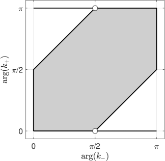
  Figure 1. The hexagonal region of $(\arg(k_{-}),\arg(k_{+}))$ where the uniqueness condition from Theorem 6.1 holds, in the case of non-magnetic materials. For such, the condition reads $\hat{k}\in\text{{\rm WP}}\,(k_{-},k_{+})$, with notation from Definition 2.1.

  When also the PDE problem defines a Fredholm map, something that can fail in the hexagon only when $|\arg(k_{+})-\arg(k_{-})|=\pi/2$, then we also have existence of solutions. Outside this region of existence and uniqueness, and for a given $k_{-}$, the uniqueness of solutions fails only for a discrete set of $k_{+}$.

• The Dirac BIE, presented in Section 2, is only one possible choice from a family of Dirac BIEs derived in Sections 7 and 8. In ${\mathbf{R}}^{2}$, these BIEs depend on four Dirac parameters $r,\beta,\alpha^{\prime},\beta^{\prime}$. The choice for $r$ is critical for numerical performance, whereas the precise choices for the other parameters seem to be of lesser importance as long as they are chosen so that no false eigenwavenumbers appear. In ${\mathbf{R}}^{3}$, there are two additional parameters $\gamma,\gamma^{\prime}$.

  The Dirac BIE is constructed in Propositions 7.3 and 8.5 using a dual PDE problem as ansatz. Our choice of dual PDE problem giving the Dirac BIEs in Section 2, has to effect that these BIEs are invertible whenever the PDE problem is well posed.

• Propositions 6.2 and 8.3 show that the PDE problem defines a Fredholm map provided that the quotient $\hat{\epsilon}$ of the permittivities is not in an interval $[-C,-1/C]$ for some $C\geq 1$ depending on the Lipschitz regularity of the interface. These estimates use Hodge potentials for the fields and concern the physical energy norm, corresponding to a boundary function space, ${\mathcal{H}}_{2}$ or ${\mathcal{H}}_{3}$, which roughly speaking is a suitable mix of the function space $H^{1/2}(\partial\Omega)\subset L_{2}(\partial\Omega)$ of traces to Sobolev $H^{1}(\Omega)$ functions and its dual space $H^{-1/2}(\partial\Omega)\supset L_{2}(\partial\Omega)$. In the case of pure metamaterials $\hat{\epsilon}<0$, the PDE problem to be solved may fail to be a Fredholm map, and hence no integral equation for solving it can be Fredholm. However, when the PDE problem has unique solution we can solve it by an injective Dirac integral equation, and when Fredholmness fails we solve the PDE problem numerically for smooth boundary data by taking a limit from $\text{{\rm Im}}\,\hat{\epsilon}>0$. Numerical experiments indicate the existence of this limit. Theoretically it should be possible to prove its existence by analyzing the problem in slightly larger fractional Sobolev spaces.

  More precisely, in ${\mathbf{R}}^{n}$, $n\geq 2$, one can show that the PDE problem (4) defines a Fredholm map when $(\hat{\epsilon}+1)/(\hat{\epsilon}-1)$ is outside the essential spectrum of the double layer potential operator

  (1) $$K_{\rm d}f(x):=\int_{\partial\Omega}\langle\nu(y),(\nabla\Phi)(y-x)\rangle f(y)d\sigma(y),\qquad x\in\partial\Omega,$$

  where $\Phi$ is the Laplace fundamental solution and $\nu$ is the outward unit normal. Another basic operator for the Maxwell problem (14) in ${\mathbf{R}}^{3}$ is the magnetic dipole operator

  (2) $$K_{\rm m}f(x):=\nu(x)\times\int_{\partial\Omega}(\nabla\Phi)(y-x)\times f(y)d\sigma(y),\qquad x\in\partial\Omega,$$

  acting on tangential vector fields $f$. Compact perturbations of the operators $K_{\rm d}$ and $K_{\rm m}$, and their adjoints $K_{\rm d}^{*}$ and $K_{\rm m}^{*}$ with respect to the standard $L_{2}$ pairing on $\partial\Omega$, appear along the diagonals of our basic Cauchy integral operators (53) and (55). In particular, the (3:4,3:4) and (7:8,7:8) size $2\times 2$ diagonal blocks in (55) are compact perturbations of $-K_{\rm m}^{*}$.

  It is important to note that in the energy norm, the essential spectra of $K_{\rm d}$ and $K_{\rm m}$ are subsets of $(-1,1)$. If considering instead the $L_{2}(\partial\Omega)$ norm, then on domains in ${\mathbf{R}}^{2}$ with one corner, the essential spectrum of $K_{\rm d}$ is a lying “figure eight”, centered around $0$. See Fabes, Jodeit and Lewis [14] and the final comments and (137) in the present paper.

• Although our main concern is wavenumbers $k_{\pm}\neq 0$, it is important to have a good behaviour of the BIEs as frequency $\omega\to 0$. Typical problems which can occur are dense-mesh low-frequency breakdown and topological low-frequency breakdown. We refer to [41, 13] for a more detailed discussion and for BIEs that are immune to such low-frequency breakdown, and remark that this immunity is shared by the Dirac BIEs presented in Section 2. One reason for this is that our four densities include the gradient of the field in ${\mathbf{R}}^{2}$ and our eight densities include the electric and the magnetic fields in ${\mathbf{R}}^{3}$, so that no numerical differentiation is needed. Moreover, if $k_{\pm}\to 0$ with $\hat{k}$ constant in (10) or (20), then $P,P^{\prime},N,N^{\prime}$ are all constant whereas the Cauchy singular integral operators $E_{k_{\pm}}$ converge to $E_{0}$ in operator norm. That the limit Dirac BIE does not have any false eigenwavenumbers, for fixed $0<|\hat{k}|<\infty$ as $k_{\pm}\to 0$, is shown in [24, Sec. 7].

  We remark that BIEs derived from the Picard system [40, 39] do not suffer from dense-mesh low-frequency breakdown, but are known to have false/near-false eigenwavenumbers. See [41, p. 163] for an excellent survey of such “charge-current formulations”. Note that the Picard equation [39, eq. (45)] is the Dirac equation (41) written in matrix form, and that the BIEs [39, eqs. (43),(44)] are $8\times 8$ systems of the second kind with single and double potential type operator blocks. Thus there is much formal resemblance with the Dirac BIE, but the real difference lies in the precise choice of parameters made in the present paper.

The paper ends with Section 9, where the numerical performance of the Dirac integral equations is studied in ${\mathbf{R}}^{2}$. Among other things, the performance is compared to that of a state-of-the-art system of integral equations of direct (Green’s theorem method) type [27, 23] which is only applicable in ${\mathbf{R}}^{2}$, which involves only two unknown scalar densities, and which for certain $k_{\pm}$ coincides with a 2D version of the classic Müller system[32, p. 319]. Not surprisingly this special-purpose system performs best, but the new $4\times 4$ Dirac system is not far behind. In particular it performs well under computationally challenging plasmonic conditions, that is when $\hat{\epsilon}$ is negative and real.

In the companion paper [24] by the authors joint with A. Karlsson, we test the new $8\times 8$ Dirac system for the Maxwell transmission problem in ${\mathbf{R}}^{3}$ using the numerical techniques in [20]. All BIE systems that we are aware of in the literature, with size less than $8\times 8$, exhibit false eigenwavenumbers – primarily at the left middle corner point in Figure 1. Our Theorem 2.3 gives very weak sufficient conditions for our Dirac integral equation (20) not to have false eigenwavenumbers. When these conditions fail, notably at the bottom middle corner point in Figure 1, it is still possible to avoid false eigenwavenumbers with other choices of Dirac parameters in Section 8.

2. Matrix Dirac integrals

This section states, in classical vector and matrix notation, the integral equations which we propose for solving the Maxwell transmission problems. The derivation of these equations in later sections makes use of multivector algebra. We consider a bounded interior domain $\Omega^{+}$, separated by the interface $\partial\Omega$ from the exterior domain $\Omega^{-}:={\mathbf{R}}^{n}\setminus\overline{\Omega^{+}}$. Fix a large $R<\infty$ and define $\Omega^{-}_{R}:=\{x\in\Omega^{-}\,\mathchar 12347\relax\,|x|<R\}$. For simplicity we assume throughout this paper that $\Omega^{-}$ is connected, although many results do not need this assumption.

The parameters that we use for problem description in the transmission problems (4) and (14), that we aim to solve, are wavenumbers $k_{+}$ and $k_{-}$ in $\Omega^{+}$ and $\Omega^{-}$ respectively, and a jump parameter $\hat{\epsilon}$. We assume that $\text{{\rm Im}}\,k_{\pm}\geq 0$, but unless otherwise stated we do not assume any relation between $k_{+},k_{-}$ and $\hat{\epsilon}$. We denote the ratio between the wavenumbers by $\hat{k}=k_{+}/k_{-}$. Our main interest is in scattering for non-magnetic materials where $\hat{\epsilon}=\hat{k}^{2}$. In applications, the parameter $\hat{\epsilon}$ appears as the ratio $\hat{\epsilon}=\epsilon_{+}/\epsilon_{-}$ of the permittivities $\epsilon_{\pm}$ in $\Omega^{\pm}$. Similarly for magnetic materials, we have a ratio $\hat{\mu}=\mu_{+}/\mu_{-}$ of the permeabilities $\mu_{\pm}$ in $\Omega^{\pm}$. In this general case, we have the relation $\hat{\epsilon}=\hat{k}^{2}/\hat{\mu}$.

We remark that in what follows, $E^{\pm}$ denotes the standard electric fields, but we have rescaled the magnetic fields $B^{\pm}$ so that what we here call $B^{\pm}$, in standard notation reads $B^{\pm}/\sqrt{\epsilon_{\pm}\mu_{\pm}}$.

To formulate our results, we need the following conical subsets of ${\mathbf{C}}$. We use the argument $-\pi<\arg(z)\leq\pi$.

Definition 2.1.

Let $k_{-},k_{+}\in{\mathbf{C}}\setminus\{0\}$ be such that $\text{{\rm Im}}\,k_{-}\geq 0$ and $\text{{\rm Im}}\,k_{+}\geq 0$. Define $\phi_{\pm}:=|\arg(k_{\pm}/i)|$. Let $\text{{\rm WP}}\,(k_{-},k_{+})\subset{\mathbf{C}}\setminus\{0\}$ be the set of $z\in{\mathbf{C}}\setminus\{0\}$ satisfying

(3) $$\begin{cases}|\arg(z)|\leq\pi-\phi_{+}-\phi_{-},&\text{if }\phi_{+}<\pi/2,\phi_{+}+\phi_{-}>0,\\ |\arg(z)|<\pi,&\text{if }\phi_{+}=\phi_{-}=0,\\ \min(|\arg(z)|,|\arg(-z)|)\leq\pi/2-\phi_{-},&\text{if }\phi_{+}=\pi/2,0<\phi_{-}\leq\pi/2,\\ \operatorname{Re}z\neq 0,&\text{if }\phi_{+}=\pi/2,\phi_{-}=0.\end{cases}$$

Our notation is to denote fields in the domains by $F,U,\ldots$, with suitable superscript $\pm$, and to write $f,u,\ldots$ for respective boundary traces. On $\partial\Omega$ we denote by $\nu$ the unit normal vector pointing into the exterior domain $\Omega^{-}$. Furthermore $\{\nu,\tau\}$ and $\{\nu,\tau,\theta\}$ denote positive ON-frames on $\partial\Omega$ depending on dimension, so that $\tau$ is the counter-clockwise tangent on curves $\partial\Omega\subset{\mathbf{R}}^{2}$. On surfaces $\partial\Omega\subset{\mathbf{R}}^{3}$, the theory we develop works for any choice of tangent ON-frame $\{\tau,\theta\}$. We denote the directional derivative in direction $v$ by $\partial_{v}$, and with slight abuse of notation , $\partial_{\nu}u$ denotes normal derivative on $\partial\Omega$ although this use values of $U$ in a neighbourhood of $\partial\Omega$.

Our main result for 2D scattering concerns the Helmholtz transmission problem

(4) $$\begin{cases}u^{+}=u^{-}+u^{0},&x\in\partial\Omega,\\ \partial_{\nu}u^{+}={\hat{\epsilon}}\partial_{\nu}(u^{-}+u^{0}),&x\in\partial\Omega,\\ \Delta U^{+}+k_{+}^{2}U^{+}=0,&x\in\Omega^{+},\\ \Delta U^{-}+k_{-}^{2}U^{-}=0,&x\in\Omega^{-},\\ \partial_{x/|x|}U^{-}-ik_{-}U^{-}=o(|x|^{-(n-1)/2}e^{\text{{\rm Im}}\,k_{-}|x|}),&x\to\infty,\end{cases}$$

where $\Omega^{+}\subset{\mathbf{R}}^{2}$, $n=2$, and with $u^{0}\in H^{1/2}(\partial\Omega)$ being the trace of an incoming wave $U^{0}$, and we want to solve for $U^{+}\in H^{1}(\Omega^{+})$ and $U^{-}\in H^{1}(\Omega^{-}_{R})$. We remark that for $\text{{\rm Im}}\,k_{-}>0$, this not so well-known sufficient radiation condition of exponential growth entails a necessary condition of exponential decay. See [37, Prop. 9.3.6] for proofs.

Let $\text{{\rm diag}}\,D$ denote the square diagonal matrix with diagonal $D$, and let $A^{\rm T}$ denote the transpose of a matrix $A$. Define

(5) $$P =\text{{\rm diag}}\,\begin{bmatrix}(\hat{k}+|\hat{k}|)^{-1/2}&(\hat{k}+|\hat{k}|)^{-1/2}&({\hat{\epsilon}}+1)^{-1}&1\end{bmatrix},$$

(6) $$P^{\prime} =\text{{\rm diag}}\,\begin{bmatrix}(\hat{k}+|\hat{k}|)^{-1/2}&(\hat{k}+|\hat{k}|)^{-1/2}&1&|\hat{k}|(\hat{k}+|\hat{k}|)^{-1}\end{bmatrix},$$

(7) $$N =\text{{\rm diag}}\,\begin{bmatrix}\hat{k}(\hat{k}+|\hat{k}|)^{-1/2}&|\hat{k}|(\hat{k}+|\hat{k}|)^{-1/2}&{\hat{\epsilon}}({\hat{\epsilon}}+1)^{-1}&1\end{bmatrix},$$

(8) $$N^{\prime} =\text{{\rm diag}}\,\begin{bmatrix}|\hat{k}|(\hat{k}+|\hat{k}|)^{-1/2}&\hat{k}(\hat{k}+|\hat{k}|)^{-1/2}&1&\hat{k}(\hat{k}+|\hat{k}|)^{-1}\end{bmatrix}.$$

Theorem 2.2.

Let $\Omega^{+}\subset{\mathbf{R}}^{2}$ be a bounded Lipschitz domain, with $\Omega^{-}$ being connected and notation as above. Then there exists a constant $1\leq C(\partial\Omega)<\infty$ depending on the Lipschitz constants of the parametrizations of $\Omega^{+}$ by smooth domains, so the following holds.

The transmission problem (4) is well posed if

(9) $${\hat{\epsilon}}\in{\mathbf{C}}\setminus[-C(\partial\Omega),-1/C(\partial\Omega)]\quad\text{and}\quad{\hat{\epsilon}}/\hat{k}\in\text{{\rm WP}}\,(k_{-},k_{+}).$$

For its solution, consider the Dirac integral equation

(10) $$(I+PE_{k_{+}}N^{\prime}-NE_{k_{-}}P^{\prime})h=2Nf^{0}$$

for four scalar functions $h=[h_{1}\;h_{2}\;h_{3}\;h_{4}]^{\rm T}$, where $E_{k}$ is the singular integral operator (53) which we introduce in Section 4, $P,P^{\prime},N,N^{\prime}$ are the constant diagonal matrices (5)–(8), and

(11) $$f^{0}=\begin{bmatrix}ik_{-}u^{0}&0&\partial_{\nu}u_{0}&\partial_{\tau}u_{0}\end{bmatrix}^{\rm T}.$$

The operator in (10) is invertible on the energy trace space ${\mathcal{H}}_{2}$ from (63), introduced in Section 7, whenever (9) holds and $\hat{k}\in{\mathbf{C}}\setminus(-\infty,0]$. Moreover, the solution to (4) in $\Omega^{\pm}$ is obtained from $h^{+}=N^{\prime}h$ and $h^{-}=P^{\prime}h$ as

(12) $$U^{\pm}=\tfrac{1}{2ik_{\pm}}\begin{bmatrix}-\tilde{K}^{\nu^{\prime}}_{k_{\pm}}&-\tilde{K}^{\tau^{\prime}}_{k_{\pm}}&\tilde{S}^{1}_{k_{\pm}}&0\end{bmatrix}h^{\pm}$$

and

(13) $$\nabla U^{\pm}=\tfrac{1}{2}\begin{bmatrix}\tilde{S}^{\nu^{\prime}}_{k_{\pm}}&\tilde{S}^{\tau^{\prime}}_{k_{\pm}}&-\tilde{K}^{I}_{k_{\pm}}&-\tilde{K}^{J}_{k_{\pm}}\end{bmatrix}h^{\pm},$$

with notation as in Section 4, where $\tilde{K}$ and $\tilde{S}$ denote layer potentials, $\nu^{\prime}$ and $\tau^{\prime}$ denote the normal and tangential vector at the point of integration $y\in\partial\Omega$, and $I=\begin{bmatrix}1&0\\ 0&1\end{bmatrix}$ and $J=\begin{bmatrix}0&-1\\ 1&0\end{bmatrix}$.

Proof.

This result is derived in Sections 6 and 7, where we arrive at equation (103) with $\alpha={\hat{\epsilon}}$. We precondition (103) by multiplying from the left by $P$ and writing $\tilde{h}=P^{\prime}h$ to obtain (10) with $N=PM$, $N^{\prime}=\hat{k}M^{\prime}P^{\prime}$ and $P(\hat{k}M^{\prime}+M)P^{\prime}=I$. We remark that the parameter ratios $\hat{k}<0$ and ${\hat{\epsilon}}=-1$ must be excluded for $P$ and $P^{\prime}$ to be well-defined. However, the only problem when $\hat{k}<0$ is that we cannot precondition (103) with $P$ and $P^{\prime}$ to achieve a non-integral term $I$ in (10).

In applications of the Dirac problem (58) to the Helmholtz problem (4), as in Example 7.1, we have $f^{0}=ik_{-}u^{0}+\nabla u^{0}$, that is (11). Equations (12) and (13) for the fields are seen from the first row and the last two rows in (53) respectively, and the expressions for $h^{\pm}$ are seen from the right and middle factors in (95). Note that $h^{-}$ happens to coincide with the density $\tilde{h}$, which is introduced in (98) in a different context. ∎

We remark that it is our experience that the precise choice of $P$ and $P^{\prime}$ for Theorem 2.2, as well as for Theorem 2.3, is less important as long as they satisfy $P(\hat{k}M^{\prime}+M)P^{\prime}=I$. With the choices made, our aim has been to minimize the growth of $P$, $P^{\prime}$, $N$ and $N^{\prime}$ as we vary $|k|$.

We next formulate the analogous result for the Maxwell transmission problem in ${\mathbf{R}}^{3}$. Our transmission problem is

(14) $$\begin{cases}\nu\times E^{+}=\nu\times(E^{-}+E^{0}),&x\in\partial\Omega,\\ \nu\times B^{+}=(\hat{k}/\hat{\epsilon})\nu\times(B^{-}+B^{0}),&x\in\partial\Omega,\\ \nabla\times E^{+}=ik_{+}B^{+},\nabla\times B^{+}=-ik_{+}E^{+},&x\in\Omega^{+},\\ \nabla\times E^{-}=ik_{-}B^{-},\nabla\times B^{-}=-ik_{-}E^{-},&x\in\Omega^{-},\\ x/|x|\times E^{-}-B^{-}=o(|x|^{-1}e^{\text{{\rm Im}}\,k_{-}|x|}),&x\to\infty,\\ x/|x|\times B^{-}-E^{-}=o(|x|^{-1}e^{\text{{\rm Im}}\,k_{-}|x|}),&x\to\infty,\\ \end{cases}$$

where $E^{0}$ and $B^{0}$ are the incoming electric and magnetic fields, and we want to solve for $E^{\pm}$ and $B^{\pm}$. All fields are assumed to be $L_{2}$ integrable in a neighbourhood of $\partial\Omega$.

Define matrices (where we write $\hat{c}=1/\hat{k}$ and $\hat{\mu}=\hat{k}^{2}/\hat{\epsilon}$)

(15) $$P =\text{{\rm diag}}\,\begin{bmatrix}\frac{1}{{\hat{c}}+1}&\frac{1}{\sqrt{{\hat{c}}+|{\hat{c}}|}}&\frac{1}{{\hat{\mu}}+1}\frac{1}{\sqrt{\hat{c}}}&\frac{1}{{\hat{\mu}}+1}\frac{1}{\sqrt{\hat{c}}}&\frac{|{\hat{c}}|}{{\hat{c}}+|{\hat{c}}|}&\frac{\hat{\epsilon}}{\hat{\epsilon}+1}&1&1\end{bmatrix},$$

(16) $$P^{\prime} =\text{{\rm diag}}\,\begin{bmatrix}1&\frac{1}{\sqrt{{\hat{c}}+|{\hat{c}}|}}&\frac{1}{\sqrt{\hat{c}}}&\frac{1}{\sqrt{\hat{c}}}&1&1&\frac{1}{{\hat{c}}+1}&\frac{1}{{\hat{c}}+1}\end{bmatrix},$$

(17) $$N =\text{{\rm diag}}\,\begin{bmatrix}\frac{{\hat{c}}}{{\hat{c}}+1}&\frac{\hat{c}}{\sqrt{{\hat{c}}+|{\hat{c}}|}}&\frac{{\hat{\mu}}}{{\hat{\mu}}+1}{\sqrt{\hat{c}}}&\frac{{\hat{\mu}}}{{\hat{\mu}}+1}{\sqrt{\hat{c}}}&\frac{{\hat{c}}}{{\hat{c}}+|{\hat{c}}|}&\frac{1}{{\hat{\epsilon}}+1}&1&1\end{bmatrix},$$

(18) $$N^{\prime} =\text{{\rm diag}}\,\begin{bmatrix}1&\frac{|{\hat{c}}|}{\sqrt{{\hat{c}}+|{\hat{c}}|}}&\sqrt{\hat{c}}&\sqrt{\hat{c}}&1&1&\frac{\hat{c}}{{\hat{c}}+1}&\frac{\hat{c}}{{\hat{c}}+1}\end{bmatrix}.$$

Theorem 2.3.

Let $\Omega^{+}\subset{\mathbf{R}}^{3}$ be a bounded Lipschitz domain, with $\Omega^{-}$ being connected and notation as above. Then there exists a constant $1\leq C(\partial\Omega)<\infty$ depending on the Lipschitz constants of the parametrizations of $\Omega^{+}$ by smooth domains, so the following holds.

The transmission problem (14) is well posed if

(19) $${\hat{\epsilon}}\in{\mathbf{C}}\setminus[-C(\partial\Omega),-1/C(\partial\Omega)]\quad\text{and}\quad{\hat{\epsilon}}/\hat{k}\in\text{{\rm WP}}\,(k_{-},k_{+}).$$

For its solution, consider the Dirac integral equation

(20) $$(I+PE_{k_{+}}N^{\prime}-NE_{k_{-}}P^{\prime})h=2Nf^{0}$$

for eight scalar functions $h=[h_{1}\;h_{2}\;h_{3}\;h_{4}\;h_{5}\;h_{6}\;h_{7}\;h_{8}]^{\rm T}$, where $E_{k}$ is the singular integral operator (55) which we introduce in Section 4, $P,P^{\prime},N,N^{\prime}$ are the constant diagonal matrices (15)–(18), and

(21) $$f^{0}=\begin{bmatrix}0&B^{0}_{\nu}&B^{0}_{\tau}&B^{0}_{\theta}&0&E^{0}_{\nu}&E^{0}_{\tau}&E^{0}_{\theta}\end{bmatrix}^{\rm T},$$

with field components in the frame $\{\nu,\tau,\theta\}$. The operator in (20) is invertible on the energy trace space ${\mathcal{H}}_{3}$ from (64), introduced in Section 8, whenever (19), ${\hat{k}}^{2}/\hat{\epsilon}\in{\mathbf{C}}\setminus[-C(\partial\Omega),-1/C(\partial\Omega)]$ and $\hat{k}\in{\mathbf{C}}\setminus(-\infty,0]$ holds. Moreover, the solution to (14) in $\Omega^{\pm}$ is obtained from $h^{+}=N^{\prime}h$ and $h^{-}=P^{\prime}h$ as

(22) $$B^{\pm}=\tfrac{1}{2}\begin{bmatrix}\tilde{K}_{k_{\pm}}^{\nu^{\prime}\times\cdot}&-\tilde{K}_{k_{\pm}}^{I}&-\tilde{K}_{k_{\pm}}^{\theta^{\prime}\times\cdot}&\tilde{K}_{k_{\pm}}^{\tau^{\prime}\times\cdot}&\tilde{S}_{k_{\pm}}^{\nu^{\prime}}&0&\tilde{S}_{k_{\pm}}^{\theta^{\prime}}&-\tilde{S}_{k_{\pm}}^{\tau^{\prime}}\end{bmatrix}h^{\pm}$$

and

(23) $$E^{\pm}=\tfrac{1}{2}\begin{bmatrix}\tilde{S}_{k_{\pm}}^{\nu^{\prime}}&0&-\tilde{S}_{k_{\pm}}^{\theta^{\prime}}&\tilde{S}_{k_{\pm}}^{\tau^{\prime}}&-\tilde{K}_{k_{\pm}}^{\nu^{\prime}\times\cdot}&-\tilde{K}_{k_{\pm}}^{I}&-\tilde{K}_{k_{\pm}}^{\theta^{\prime}\times\cdot}&\tilde{K}_{k_{\pm}}^{\tau^{\prime}\times\cdot}\end{bmatrix}h^{\pm},$$

with notation as in Section 4, where $\tilde{K}$ and $\tilde{S}$ denote layer potentials, $\nu^{\prime},\tau^{\prime},\theta^{\prime}$ denote the frame vectors at the point of integration $y\in\partial\Omega$, $I=\begin{bmatrix}1&0\\ 0&1\end{bmatrix}$, and $v\times\cdot$ denotes the map $x\mapsto v\times x$.

Proof.

This result is derived in Section 8, where we arrive at equation (133) with $\alpha=\hat{\epsilon}$. We precondition (133) by multiplying from the left by $P$ and writing $\tilde{h}=P^{\prime}h$ to obtain (20) with $N=PM$, $N^{\prime}=\hat{k}^{-1}M^{\prime}P^{\prime}$ and $P(\hat{k}^{-1}M^{\prime}+M)P^{\prime}=I$. We remark that the parameter ratios $\hat{k}<0$, $\hat{\mu}={\hat{k}}^{2}/\hat{\epsilon}=-1$ and ${\hat{\epsilon}}=-1$ must be excluded for $P$ and $P^{\prime}$ to be well-defined. However, the only problem when $\hat{k}<0$ is that we cannot precondition (133) with $P$ and $P^{\prime}$ to achieve a non-integral term $I$ in (20).

In applications of the Dirac problem (58) to the Maxwell problem (14), or in multivector notation (107), we have $F^{0}=E^{0}+B^{0}$, that is (21). Equations (22) and (23) for the fields are seen from the second to fourth rows and last three rows in (55) respectively. ∎

3. Multivector algebra

This section contains the basics of multivector algebra which we need. For a complete account of the theory of multivector algebra and Dirac equations which we use, we refer to [37]. For our purposes, multivectors are the same objects as Cartan’s alternating forms, and multivector fields are the same as differential forms, and amounts to an algebra of not only the one-dimensional vectors but also $j$-dimensional algebraic objects for $0\leq j\leq n$ in ${\mathbf{R}}^{n}$. Concretely, multivectors in ${\mathbf{R}}^{n}$ are the following type of objects, where our interest is in $n=2,3$. Denote by $\{e_{1},\ldots,e_{n}\}$ the standard vector basis for ${\mathbf{R}}^{n}$. We write $\wedge{\mathbf{R}}^{n}$ for the complex $2^{n}$ dimensional space of multivectors in ${\mathbf{R}}^{n}$, which is spanned by basis multivectors $e_{s}$, where $s\subset{\overline{n}}=\{1,2,\ldots,n\}$. We write $\wedge^{j}{\mathbf{R}}^{n}$ for the subspace spanned by those $e_{s}$ with $j$ number of elements in the index set $s$, so that

(24) $$\wedge{\mathbf{R}}^{n}=\wedge^{0}{\mathbf{R}}^{n}\oplus\wedge^{1}{\mathbf{R}}^{n}\oplus\wedge^{2}{\mathbf{R}}^{n}\oplus\cdots\oplus\wedge^{n}{\mathbf{R}}^{n}.$$

We identify $\wedge^{0}{\mathbf{R}}^{n}={\mathbf{C}}$ and $\wedge^{1}{\mathbf{R}}^{n}={\mathbf{C}}^{n}$ with the scalars and vectors respectively. Objects in $\wedge^{2}{\mathbf{R}}^{n}$ are referred to as bivectors.

In ${\mathbf{R}}^{2}$, a multivector is of the form

(25) $$w=a+v_{1}e_{1}+v_{2}e_{2}+be_{12},$$

and so amounts to two scalars $a,b$ and a vector $v=v_{1}e_{1}+v_{2}e_{2}$. In ${\mathbf{R}}^{3}$, a multivector is of the form

(26) $$w=a+v_{1}e_{1}+v_{2}e_{2}+v_{3}e_{3}+u_{1}e_{23}+u_{2}e_{13}+u_{3}e_{12}+be_{123},$$

and so amounts to two scalars $a,b$ and two vectors $v=v_{1}e_{1}+v_{2}e_{2}+v_{3}e_{3}$ and $u=u_{1}e_{1}+u_{2}e_{2}+u_{3}e_{3}$ via Hodge duality (see below).

On this $2^{n}$ dimensional space $\wedge{\mathbf{R}}^{n}$ we use three products which, depending on dimension, generalize the classical vector operations: the exterior product $u\mathbin{\scriptstyle{\wedge}}w$, the (left) interior product $u\mathbin{\lrcorner}w$ and the Clifford product $uw$. The last is the standard short hand notation for the Clifford product, whereas the notation $e_{s}\mathbin{\scriptscriptstyle{\triangle}}e_{t}$ was introduced in [37], for reasons which are clear from (29). Products of basis multivectors $e_{s}$ correspond to signed unions, set differences and symmetric differences of index sets $s$ respectively. More precisely, for index sets $s,t\subset{\overline{n}}$ we define the permutation sign $\epsilon(s,t)=(-1)^{|\{(s_{i},t_{j})\in s\times t\,\mathchar 12347\relax\,s_{i}>t_{j}\}|}$, that is the sign of the permutation that rearranges $s\cup t$ in increasing order. Then

(27) $$e_{s}\mathbin{\scriptstyle{\wedge}}e_{t} =\begin{cases}\epsilon(s,t)e_{s\cup t},&s\cap t=\emptyset,\\ 0,&s\cap t\neq\emptyset,\end{cases}$$

(28) $$e_{s}\mathbin{\lrcorner}e_{t} =\begin{cases}0,&s\not\subseteq t,\\ \epsilon(s,t\setminus s)e_{t\setminus s},&s\subseteq t,\end{cases}$$

(29) $$e_{s}e_{t} =\epsilon(s,t)e_{s\triangle t},$$

where $s\triangle t=(s\cup t)\setminus(s\cap t)$ is the symmetric difference of sets. The exterior and Clifford products are associative, but the interior product is not. On the one hand, orthogonal vectors in $\wedge^{1}{\mathbf{R}}^{n}$ anticommute both with respect to the exterior and Clifford products. On the other hand, $e_{j}\mathbin{\scriptstyle{\wedge}}e_{j}=0$ whereas $e_{j}e_{j}=1$, $j=1,\ldots,n$. An important special case of the interior product is the Hodge star duality

(30) $${*w}=w\mathbin{\lrcorner}e_{\overline{n}}.$$

The most important instance of the above three products is when the first factor is a vector, and not a general multivector. In this case, the three products are related as

(31) $$uw=u\mathbin{\lrcorner}w+u\mathbin{\scriptstyle{\wedge}}w,\qquad u\in\wedge^{1}{\mathbf{R}}^{n},w\in\wedge{\mathbf{R}}^{n}.$$

A multivector $w\in\wedge{\mathbf{R}}^{n}$ at a point $x\in\partial\Omega$, with normal vector $\nu\in\wedge^{1}{\mathbf{R}}^{n}$, is called tangential if $\nu\mathbin{\lrcorner}w=0$ and is called normal if $\nu\mathbin{\scriptstyle{\wedge}}w=0$.

Example 3.1 (${\mathbf{R}}^{2}$ multivector algebra).

A general multivector in ${\mathbf{R}}^{2}$ is of the form $w=a_{1}+v+*a_{2}$, where $a_{1},a_{2}\in\wedge^{0}{\mathbf{R}}^{2}$ and $v\in\wedge^{1}{\mathbf{R}}^{2}$. The three basic multivector products with a vector $u\in\wedge^{1}{\mathbf{R}}^{2}$ can be written

(32) $$u\mathbin{\scriptstyle{\wedge}}w =0+a_{1}u+*((*u)\cdot v),$$

(33) $$u\mathbin{\lrcorner}w =u\cdot v+a_{2}(*u)+0,$$

(34) $$uw =u\cdot v+(a_{1}u+a_{2}(*u))+*((*u)\cdot v).$$

Note that on vectors $u\in\wedge^{1}{\mathbf{R}}^{2}$, the Hodge star $*u$ is counter clockwise rotation $\pi/2$.

Example 3.2 (${\mathbf{R}}^{3}$ multivector algebra).

A general multivector in ${\mathbf{R}}^{3}$ is of the form $w=a_{1}+v_{1}+*v_{2}+*a_{2}$, where $a_{1},a_{2}\in\wedge^{0}{\mathbf{R}}^{3}$ and $v_{1},v_{2}\in\wedge^{1}{\mathbf{R}}^{3}$. The three basic multivector products with a vector $u\in\wedge^{1}{\mathbf{R}}^{3}$ can be written

(35) $$u\mathbin{\scriptstyle{\wedge}}w =0+ua_{1}+*(u\times v_{1})+*(u\cdot v_{2}),$$

(36) $$u\mathbin{\lrcorner}w =u\cdot v_{1}-u\times v_{2}+*(ua_{2})+0,$$

(37) $$uw =u\cdot v_{1}+(ua_{1}-u\times v_{2})+*(u\times v_{1}+ua_{2})+*(u\cdot v_{2}).$$

We refer to [37, Chapters 2,3] for further details of multivector algebra.

In the same way that the scalar and vector products induce the divergence $\nabla\cdot F$ and curl $\nabla\times F$ in vector calculus, the exterior, interior and Clifford products induce the exterior, interior and Clifford/Dirac derivatives in multivector calculus, and we write these as

(38) $$dF(x)=\nabla\mathbin{\scriptstyle{\wedge}}F(x) =\sum_{j=1}^{n}e_{j}\mathbin{\scriptstyle{\wedge}}\partial_{e_{j}}F(x),$$

(39) $$\delta F(x)=\nabla\mathbin{\lrcorner}F(x) =\sum_{j=1}^{n}e_{j}\mathbin{\lrcorner}\partial_{e_{j}}F(x),$$

(40) $${\mathbf{D}}F(x)=\nabla\mathbin{\scriptscriptstyle{\triangle}}F(x) =\sum_{j=1}^{n}e_{j}\partial_{e_{j}}F(x).$$

Replacing $u$ and $w$ by $\nabla$ and $F(x)$ in Example 3.2, it follows how these differential operators can be written in terms of divergence, curl and gradient in ${\mathbf{R}}^{3}$. We refer to [37, Chapters 7,8] for further details of multivector calculus.

The time-harmonic wave Dirac equation which we consider in this paper is

(41) $${\mathbf{D}}F(x)=ikF(x),$$

for multivector fields $F$, and wave number $k\in{\mathbf{C}}$. The main applications are the Helmholtz and Maxwell equations. Given a scalar solution $U$ to the Helmholtz equation $\Delta U+k^{2}U=0$, we define the multivector field

(42) $$F_{\text{helm}}=\nabla U+ikU.$$

It follows that $F=F_{\text{helm}}$ satisfies (41) since ${\mathbf{D}}^{2}=\Delta$.

For Maxwell’s equations, define the total electromagnetic (EM) field to be the multivector field

(43) $$F_{\text{{\rm em}}}\,(x)=E_{1}(x)e_{1}+E_{2}(x)e_{2}+E_{3}(x)e_{3}+B_{1}(x)e_{23}-B_{2}(x)e_{13}+B_{3}(x)e_{12},$$

where $E$ is the electric field and $B$ is the magnetic field, and the $\wedge^{0}{\mathbf{R}}^{3}$ and $\wedge^{3}{\mathbf{R}}^{3}$ parts are zero. In this formalism, the Dirac equation (41) for $F=F_{\text{{\rm em}}}\,$ given by (43) coincides with the time-harmonic Maxwell’s equations, that is the PDE from (14). Indeed, the $\wedge^{0}{\mathbf{R}}^{3}$, $\wedge^{1}{\mathbf{R}}^{3}$, $\wedge^{2}{\mathbf{R}}^{3}$ and $\wedge^{3}{\mathbf{R}}^{3}$ parts of (41) are the Gauss, Maxwell–Ampère, Faraday and magnetic Gauss law respectively. See [37, Sec. 9.2].

4. The ${\mathbf{R}}^{n}$ Cauchy integral

A main reason for using the Dirac framework is that it provides us with a Cauchy-type reproducing formula, which allows for a generalization of complex function theory to $n\geq 2$ and $k\neq 0$. See [37, Chapters 8,9] for further details. More precisely, if $F$ satisfies (41) in a domain $\Omega$ with boundary $\partial\Omega$, then a Cauchy-type reproducing formula

(44) $$F(x)=\int_{\partial\Omega}\Psi_{k}(y-x)\nu(y)f(y)d\sigma(y),\qquad x\in\Omega,$$

holds. We write $dy$ and $\nu\in\wedge^{1}{\mathbf{R}}^{n}$ for the standard measure and outward pointing unit normal on $\partial\Omega$ respectively, and the integrand uses two Clifford products. The first factor

(45) $$\Psi_{k}(x)=-\tfrac{1}{2}(\nabla\Phi_{k}(x)-ik\Phi_{k}(x))\in\wedge^{1}{\mathbf{R}}^{n}\oplus\wedge^{0}{\mathbf{R}}^{n}\subset\wedge{\mathbf{R}}^{n}$$

is a fundamental solution to the elliptic operator ${\mathbf{D}}+ik$, as ${\mathbf{D}}\Psi_{k}(x)+ik\Psi_{k}(x)=\delta(x)$. Here $\Phi_{k}(x)\in\wedge^{0}{\mathbf{R}}^{n}={\mathbf{C}}$ is the Helmholtz fundamental solution, and we use the normalization from [11] so that $(\Delta+k^{2})\Phi_{k}=-2\delta(x)$. Hence the factor $-1/2$ in (45). In dimension $n=3$ we have

(46) $$\Phi_{k}(x)=(2\pi|x|)^{-1}e^{ik|x|},$$

and in dimension $n=2$ we have in terms of the Hankel function $H^{(1)}_{0}(z)$ that

(47) $$\Phi_{k}(x)=(i/2)H^{(1)}_{0}(k|x|).$$

The classical theory of complex Hardy spaces generalizes from complex function theory to our Dirac setting. Our basic operator, acting on a suitable space ${\mathcal{H}}$ of functions $h:\partial\Omega\to\wedge{\mathbf{R}}^{n}$ on $\partial\Omega$, is the Cauchy principal value integral

(48) $$E_{k}h(x)=2\text{{\rm p.v.\!}}\int_{\partial\Omega}\Psi_{k}(y-x)\nu(y)h(y)d\sigma(y),\qquad x\in\partial\Omega,$$

which reduces to the classical Cauchy integral when $n=2$, $k=0$. The basic operator algebra is that $E_{k}^{2}=I$, and

(49) $$E_{k}^{\pm}=(I\pm E_{k})/2$$

are two complementary projection operators, that is $(E_{k}^{\pm})^{2}=E_{k}^{\pm}$. The operator $E_{k}^{\pm}$ projects onto its range, the subspace of ${\mathcal{H}}$ which we denote $E_{k}^{\pm}{\mathcal{H}}$ and consists of all traces $F|_{\partial\Omega}$ of fields satisfying ${\mathbf{D}}F=ikF$ in $\Omega^{\pm}$. For the exterior domain $\Omega^{-}$ these fields also satisfy a Dirac radiation condition; See (58) below for its formulation.

For computations, we express the Cauchy singular operator $E_{k}$ as a matrix with entries being double and single layer potential-type operators, using the notation

(50) $$K^{v}_{k}h(x) =\text{{\rm p.v.\!}}\int_{\partial\Omega}\langle v(x,y),(\nabla\Phi_{k})(y-x)\rangle h(y)d\sigma(y),\qquad x\in\partial\Omega,$$

(51) $$S^{a}_{k}h(x) =ik\int_{\partial\Omega}a(x,y)\Phi_{k}(y-x)h(y)d\sigma(y),\qquad x\in\partial\Omega,$$

respectively. Here $v(x,y)$ is a vector field and $a(x,y)$ is a scalar function, depending on $x,y\in\partial\Omega$. The single layer $S^{a}_{k}$ is a weakly singular integral operator, and so is also $K^{v}_{k}$ if $\partial\Omega$ is smooth and $v=\nu$ is the normal direction at $x$ or $y$. Otherwise $K^{v}_{k}$ is a principal value singular integral, but is bounded on many natural function spaces ${\mathcal{H}}$, also for general Lipschitz interfaces $\partial\Omega$.

Consider first dimension $n=2$, with a curve $\partial\Omega$ and $\Phi_{k}$ given by (47). Here we use a positively oriented frame $\{\nu,\tau\}$ at $x\in\partial\Omega$, with $\nu=\nu(x)$ being the normal vector into $\Omega^{-}$ and $\tau=\tau(x)$ the tangential vector counter clock-wise from $\nu$. The corresponding frame at $y\in\partial\Omega$ we write as $\nu^{\prime}=\nu(y)$ and $\tau^{\prime}=\tau(y)$. In the plane, the Clifford algebra $\wedge{\mathbf{R}}^{2}$ is four dimensional and spanned by $\{1,e_{1},e_{2},e_{12}\}$. We prefer the ordering $\{1,e_{12},e_{1},e_{2}\}$, since Clifford multiplication by vectors then will be represented by block off-diagonal matrices. At $x\in\partial\Omega$, we write

(52) $$h=h_{1}+h_{2}\nu\tau+h_{3}\nu+h_{4}\tau\approx\begin{bmatrix}h_{1}&h_{2}&h_{3}&h_{4}\end{bmatrix}^{\rm T},$$

using instead the vector frame $\{\nu,\tau\}$. Here $\nu\tau=e_{12}\in\wedge^{2}{\mathbf{R}}^{2}$ does not depend on $x$, even though $\nu$ and $\tau$ do so. By writing out $\nabla\Phi_{k}$ and the Clifford products in (48), we obtain

(53) $$E_{k}=\begin{bmatrix}-K^{\nu^{\prime}}_{k}&-K^{\tau^{\prime}}_{k}&S^{1}_{k}&0\\ K^{\tau^{\prime}}_{k}&-K^{\nu^{\prime}}_{k}&0&S^{1}_{k}\\ S^{\nu\cdot\nu^{\prime}}_{k}&S^{\nu\cdot\tau^{\prime}}_{k}&-K^{\nu}_{k}&K^{\tau}_{k}\\ S^{\tau\cdot\nu^{\prime}}_{k}&S^{\tau\cdot\tau^{\prime}}_{k}&-K^{\tau}_{k}&-K^{\nu}_{k}\end{bmatrix},$$

in the multivector frame $\{1,\nu\tau,\nu,\tau\}$.

Next consider dimension $n=3$, with a surface $\partial\Omega$ and $\Phi_{k}$ given by (46). Here we use a positively oriented ON-frame $\{\nu,\tau,\theta\}$ at $x\in\partial\Omega$, with $\nu=\nu(x)$ being the normal vector into $\Omega^{-}$ and $\tau=\tau(x)$ and $\theta=\theta(x)$ being tangential vector fields. The frame vectors at $y\in\partial\Omega$, we write as $\nu^{\prime}=\nu(y)$, $\tau^{\prime}=\tau(y)$ and $\theta^{\prime}=\theta(y)$. A multivector field at $x\in\partial\Omega$ we write as

(54) $$h=h_{1}+h_{2}\tau\theta+h_{3}\theta\nu+h_{4}\nu\tau+h_{5}\nu\tau\theta+h_{6}\nu+h_{7}\tau+h_{8}\theta.$$

Here $\nu\tau\theta=e_{123}\in\wedge^{3}{\mathbf{R}}^{3}$ does not depend on $x$, although in general each of the three vectors do so. Again, we prefer this ordering of the frame multivectors since Clifford multiplication by vectors then is block off-diagonal. In the multivector frame $\{1,\tau\theta,\theta\nu,\nu\tau,\nu\tau\theta,\nu,\tau,\theta\}$, we have

(55) $$E_{k}=\begin{bmatrix}-K^{\nu^{\prime}}_{k}&0&K^{\theta^{\prime}}_{k}&-K^{\tau^{\prime}}_{k}&0&S^{1}_{k}&0&0\\ K^{\nu\times\nu^{\prime}}_{k}&-K^{\nu}_{k}&-K^{\nu\times\theta^{\prime}}_{k}&K^{\nu\times\tau^{\prime}}_{k}&S^{\nu\cdot\nu^{\prime}}_{k}&0&S^{\nu\cdot\theta^{\prime}}_{k}&-S^{\nu\cdot\tau^{\prime}}_{k}\\ K^{\tau\times\nu^{\prime}}_{k}&-K^{\tau}_{k}&-K^{\tau\times\theta^{\prime}}_{k}&K^{\tau\times\tau^{\prime}}_{k}&S^{\tau\cdot\nu^{\prime}}_{k}&0&S^{\tau\cdot\theta^{\prime}}_{k}&-S^{\tau\cdot\tau^{\prime}}_{k}\\ K^{\theta\times\nu^{\prime}}_{k}&-K^{\theta}_{k}&-K^{\theta\times\theta^{\prime}}_{k}&K^{\theta\times\tau^{\prime}}_{k}&S^{\theta\cdot\nu^{\prime}}_{k}&0&S^{\theta\cdot\theta^{\prime}}_{k}&-S^{\theta\cdot\tau^{\prime}}_{k}\\ 0&S^{1}_{k}&0&0&-K^{\nu^{\prime}}_{k}&0&-K^{\theta^{\prime}}_{k}&K^{\tau^{\prime}}_{k}\\ S^{\nu\cdot\nu^{\prime}}_{k}&0&-S^{\nu\cdot\theta^{\prime}}_{k}&S^{\nu\cdot\tau^{\prime}}_{k}&-K^{\nu\times\nu^{\prime}}_{k}&-K^{\nu}_{k}&-K^{\nu\times\theta^{\prime}}_{k}&K^{\nu\times\tau^{\prime}}_{k}\\ S^{\tau\cdot\nu^{\prime}}_{k}&0&-S^{\tau\cdot\theta^{\prime}}_{k}&S^{\tau\cdot\tau^{\prime}}_{k}&-K^{\tau\times\nu^{\prime}}_{k}&-K^{\tau}_{k}&-K^{\tau\times\theta^{\prime}}_{k}&K^{\tau\times\tau^{\prime}}_{k}\\ S^{\theta\cdot\nu^{\prime}}_{k}&0&-S^{\theta\cdot\theta^{\prime}}_{k}&S^{\theta\cdot\tau^{\prime}}_{k}&-K^{\theta\times\nu^{\prime}}_{k}&-K^{\theta}_{k}&-K^{\theta\times\theta^{\prime}}_{k}&K^{\theta\times\tau^{\prime}}_{k}\end{bmatrix}.$$

Finally we note that we similarly can write the Cauchy integral (44) for the fields in $\Omega^{\pm}$ , in matrix form. The only difference is the normalization factor $2$ and the fact that we choose the frame $\{e_{1},\ldots,e_{n}\}$ at the field point $x\in\Omega^{\pm}$. We also allow for a general function $h:\partial\Omega\to\wedge{\mathbf{R}}^{n}$ and not only a trace $f$ of a solution to the Dirac equation in (44). By the associativity of the Clifford product, this still yields a field $F$ solving the Dirac equation, but $h\neq F|_{\partial\Omega}$ in general. In this case, when $x\notin\partial\Omega$, we denote the layer potentials by $\tilde{K}^{v}_{k}$ and $\tilde{S}^{a}_{k}$, with $v$ and $a$ now only depending on $y\in\partial\Omega$. The field evaluation formulas (13), (22) and (23) also use vector versions

(56) $$\tilde{K}^{A}_{k}h(x) =\int_{\partial\Omega}A(y)(\nabla\Phi_{k})(y-x)h(y)d\sigma(y),\qquad x\notin\partial\Omega,$$

(57) $$\tilde{S}^{v}_{k}h(x) =ik\int_{\partial\Omega}v(y)\Phi_{k}(y-x)h(y)d\sigma(y),\qquad x\notin\partial\Omega,$$

of $\tilde{K}^{v}_{k}$ and $\tilde{S}^{a}_{k}$, where now $A(y):{\mathbf{R}}^{n}\to{\mathbf{R}}^{n}$ is a matrix function and $v(y)$ is a vector field.

5. The energy trace space

We define in this section the appropriate norms and function spaces for the Dirac equation (41). Let $\Omega^{+}\subset{\mathbf{R}}^{n}$ be a bounded Lipschitz domain. The general Dirac transmission problem that we consider reads

(58) $$\begin{cases}f^{+}=M(f^{-}+f^{0}),&x\in\partial\Omega,\\ {\mathbf{D}}F^{+}=ik_{+}F^{+},&x\in\Omega^{+},\\ {\mathbf{D}}F^{-}=ik_{-}F^{-},&x\in\Omega^{-},\\ (x/|x|-1)F^{-}=o(|x|^{-(n-1)/2}e^{\text{{\rm Im}}\,k_{-}|x|}),&x\to\infty.\end{cases}$$

This is our master transmission problem, into which we embed the Helmholtz and Maxwell transmission problems in Sections 7 and 8, where the multiplier $M$ will be specified. The radiation condition stated here for the Dirac equation reduces to the classical Sommerfeld and Silver–Müller conditions for Helmholtz and Maxwell solutions $F_{\text{helm}}$ and $F_{\text{{\rm em}}}\,$ respectively. See [37, Sec. 9.3].

For $F=F^{+}$ in $\Omega^{+}$, we use the norm

(59) $$\left(\int_{\Omega^{+}}(|F(x)|^{2}+|\nabla\mathbin{\scriptstyle{\wedge}}F(x)|^{2})dx\right)^{1/2}.$$

It is important to note that for both Helmholtz and Maxwell fields $F_{\text{helm}}$ and $F_{\text{{\rm em}}}\,$, the second term $\nabla\mathbin{\scriptstyle{\wedge}}F$ is bounded by the first term $F$, and the norm reduces to the $L_{2}$ norm of $F$. In $\Omega^{-}$ we use the corresponding norm, but integrate only over the bounded set $\Omega^{-}_{R}$. Different choices of $R$ yield equivalent norms for solutions to the Dirac equation which satisfy the radiation condition. See [37, Sec. 9.3].

It was shown in [4] that there exists a unique Hilbert space ${\mathcal{H}}$ (although it does not come with a canonical norm) of multivector fields on the Lipschitz interface $\partial\Omega$, which is the trace space corresponding to the above norms on $F^{\pm}$ in $\Omega^{\pm}$, with the following properties. It splits into closed subspaces in two ways as

(60) $${\mathcal{H}}=E_{k}^{+}{\mathcal{H}}\oplus E_{k}^{-}{\mathcal{H}}\quad\text{and}\quad{\mathcal{H}}={\mathcal{H}}_{\scriptstyle\top}\oplus{\mathcal{H}}_{\scriptstyle\perp},$$

where ${\scriptstyle\top}$ means tangential and ${\scriptstyle\perp}$ means normal. There is a one-to-one correspondence $F^{+}\leftrightarrow f^{+}$ between Dirac solutions $F^{+}$ in $\Omega^{+}$ and their traces $f^{+}\in E_{k}^{+}{\mathcal{H}}$, with inverse given by the Cauchy integral (44). Similarly, there is a one-to-one correspondence $F^{-}\leftrightarrow f^{-}$ between Dirac solutions $F^{-}$ in $\Omega^{-}$ satisfying the radiation condition, and their traces $f^{-}\in E_{k}^{-}{\mathcal{H}}$, with inverse given by the Cauchy integral.

The subspace ${\mathcal{H}}_{\scriptstyle\top}$ denotes the subspace of tangential multivector fields, and there is a bounded and surjective tangential trace map

(61) $$F\mapsto\nu\mathbin{\lrcorner}(\nu\mathbin{\scriptstyle{\wedge}}f)\in{\mathcal{H}}_{\scriptstyle\top},$$

of multivector fields $F$ in a neighbourhood $U$ of $\partial\Omega$ with norm $(\int_{U}(|F(x)|^{2}+|\nabla\mathbin{\scriptstyle{\wedge}}F(x)|^{2})dx)^{1/2}<\infty$. The subspace ${\mathcal{H}}_{\scriptstyle\perp}$ denotes the subspace of normal multivector fields, and there is a bounded and surjective normal trace map

(62) $$F\mapsto\nu\mathbin{\scriptstyle{\wedge}}(\nu\mathbin{\lrcorner}f)\in{\mathcal{H}}_{\scriptstyle\perp},$$

of multivector fields $F$ in a neighbourhood $U$ of $\partial\Omega$ with norm $(\int_{U}(|F(x)|^{2}+|\nabla\mathbin{\lrcorner}F(x)|^{2})dx)^{1/2}<\infty$.

For smooth interfaces $\partial\Omega$, the trace space ${\mathcal{H}}$ consists of all $f\in H^{-1/2}(\partial\Omega;\wedge{\mathbf{R}}^{n})$ such that $d_{\scriptstyle\top}f_{\scriptstyle\top}\in H^{-1/2}(\partial\Omega;\wedge{\mathbf{R}}^{n})$ and $\delta_{\scriptstyle\top}(\nu\mathbin{\lrcorner}f)\in H^{-1/2}(\partial\Omega;\wedge{\mathbf{R}}^{n})$, with $d_{\scriptstyle\top}$ and $\delta_{\scriptstyle\top}$ denoting the tangential exterior and interior derivatives along $\partial\Omega$. Here $f_{\scriptstyle\top}$ denotes the tangential part of $f$ and $\nu\mathbin{\lrcorner}f$ is the normal part of $f$ with the factor $\nu$ removed.

To characterize ${\mathcal{H}}$ in terms of fractional Sobolev-type spaces on non-smooth Lipschitz interfaces $\partial\Omega$ is a non-trivial problem. Such a characterization was achieved for polyhedra in [7, 8], for general Lipschitz interfaces in [9] in ${\mathbf{R}}^{3}$, and extended to general multivector traces in [42]. For the energy trace space space ${\mathcal{H}}$ on Lipschitz interfaces, this shows the following. For 2D domains, using the frame (52), our boundary function space is

(63) $${\mathcal{H}}_{2}={\mathcal{H}}=H^{1/2}(\partial\Omega)\oplus H^{1/2}(\partial\Omega)\oplus H^{-1/2}(\partial\Omega)\oplus H^{-1/2}(\partial\Omega).$$

It is for 3D domains that the non-trivial result from [9, Thm. 4.1] is needed, which shows that in the frame (54), we have

(64) $${\mathcal{H}}_{3}={\mathcal{H}}=H^{1/2}(\partial\Omega)\oplus H^{-1/2}(\partial\Omega)\oplus*H^{-1/2}({\text{{\rm curl}}},\partial\Omega)\\ \qquad\oplus H^{1/2}(\partial\Omega)\oplus H^{-1/2}(\partial\Omega)\oplus H^{-1/2}({\text{{\rm curl}}},\partial\Omega).$$

Here $*$ is the 3D Hodge star and the space of tangential vector fields is defined as

(65) $$H^{-1/2}({\text{{\rm curl}}},\partial\Omega)=\{f\in(\nu\times H^{1/2}(\partial\Omega)^{3})^{*}\,\mathchar 12347\relax\,{\text{{\rm curl}}}_{\scriptstyle\top}f\in H^{-1/2}(\partial\Omega)\},$$

where ${\text{{\rm curl}}}_{\scriptstyle\top}$ denotes tangential surface curl on $\partial\Omega$ and $(\nu\times H^{1/2}(\partial\Omega)^{3})^{*}$ denotes the dual space of $\nu\times H^{1/2}(\partial\Omega)^{3}$. One should note that the test functions $\nu\times H^{1/2}(\partial\Omega)^{3}$ will not be $H^{1/2}$ smooth on general Lipschitz regular $\partial\Omega$, since $\nu$ is in general only measurable. To summarize, the conditions on $h_{3},h_{4},h_{7},h_{8}$ are that $h_{3}\tau+h_{4}\theta\in H^{-1/2}({\text{{\rm curl}}},\partial\Omega)$ and $h_{7}\tau+h_{8}\theta\in H^{-1/2}({\text{{\rm curl}}},\partial\Omega)$.

We remark that there is no canonical norm on ${\mathcal{H}}_{2}$ or ${\mathcal{H}}_{3}$, but this does not present a problem and it should be clear from the context in the estimates to come, which choice among equivalent norms is used when such needs to be fixed.

Throughout this paper $X\lesssim Y$ means that there exists $C<\infty$ independent of relevant variables so that $X\leq CY$, and $X\approx Y$ means that $X\lesssim Y$ and $Y\lesssim X$.

6. Helmholtz existence and uniqueness

This section surveys basic solvability results for the Helmholtz transmission problem (4), which are valid in any dimension $n\geq 2$. The proofs follow [4], with a translation from the Dirac to the Helmholtz framework. Consider first uniqueness of solutions $U^{\pm}$.

Proposition 6.1.

Let $\Omega^{+}\subset{\mathbf{R}}^{n}$ be a bounded Lipschitz domain with connected exterior $\Omega^{-}$, and consider a solution $U^{\pm}$ to (4). Assume that the incoming wave vanishes so that $u_{0}=0$. If $\hat{\epsilon}$ from (4) satisfies

(66) $${\hat{\epsilon}}/\hat{k}\in\text{{\rm WP}}\,(k_{-},k_{+}),$$

recalling that $\hat{k}=k_{+}/k_{-}$ and Definition 2.1, then $U^{+}=U^{-}=0$ identically.

Proof.

From the jump relations we have

(67) $$\int_{\partial\Omega}u^{+}\overline{\partial_{\nu}u^{+}}d\sigma=\overline{\hat{\epsilon}}\int_{\partial\Omega}u^{-}\overline{\partial_{\nu}u^{-}}d\sigma.$$

Apply Green’s first identity for $\Omega^{+}$ and $\Omega^{-}_{R}$, use the Helmholtz equation for $U^{\pm}$ and the radiation condition for $U^{-}$, and multiply the equation by ${\hat{\epsilon}}k_{-}/i$ to obtain

(68) $$\frac{{\hat{\epsilon}}k_{-}}{k_{+}}\left(\frac{1}{i}\int_{\Omega^{+}}(k_{+}|\nabla U^{+}|^{2}-\overline{k}_{+}|k_{+}U^{+}|^{2})dx\right)\\ +|{\hat{\epsilon}}|^{2}\left(\frac{1}{i}\int_{\Omega^{-}_{R}}(k_{-}|\nabla U^{-}|^{2}-\overline{k}_{-}|k_{-}U^{-}|^{2})dx+\int_{|x|=R}|k_{-}U^{-}|^{2}d\sigma\right)\to 0,$$

as $R\to\infty$. Denote the three integrals appearing in (68) by $I^{+}$, $I^{-}_{R}$ and $I_{R}$ respectively, including $i^{-1}$ in the first two, and set $\phi_{\pm}:=|\arg(k_{\pm}/i)|$ as in Definition 2.1, let $z:={\hat{\epsilon}}k_{-}/k_{+}$, and define the sector

(69) $$S_{\phi}:=\{z\in{\mathbf{C}}\setminus\{0\}\,\mathchar 12347\relax\,|\arg(z)|\leq\phi\}\cup\{0\}.$$

We note that

(70) $$I^{+}=\text{{\rm Im}}\,k_{+}\int_{\Omega^{+}}(|\nabla U^{+}|^{2}+|k_{+}U^{+}|^{2})dx-i\operatorname{Re}k_{+}\int_{\Omega^{+}}(|\nabla U^{+}|^{2}-|k_{+}U^{+}|^{2})dx,$$

and similarly for $I^{-}_{R}$.

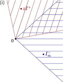
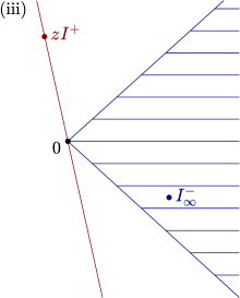
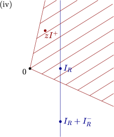
Figure 2. Sectors and lines appearing, depending on $\phi_{\pm}$.

We verify that the condition (66) implies $U^{\pm}=0$, by examining (68) in the nine cases $\phi_{\pm}=0$, $0<\phi_{\pm}<\pi/2$ and $\phi_{\pm}=\pi/2$ as follows.

(i) Assume $0<\phi_{-}<\pi/2$ and $0<\phi_{+}<\pi/2$. Then $U^{-}$ decays exponentially as $R\to\infty$. Setting $R=\infty$ in (68), we have the equation $zI^{+}+|{\hat{\epsilon}}|^{2}I^{-}_{\infty}=0$, where $I^{+}\in S_{\phi_{+}}$ and $I^{-}_{\infty}\in S_{\phi_{-}}$. If $|\arg(z)|+\phi_{-}+\phi_{+}<\pi$, then this is possible only if $I^{+}=I^{-}_{\infty}=0$. See Figure 2(i). Indeed, the sectors $zS_{\phi_{+}}$ and $-S_{\phi_{-}}$ intersect only at $0$. We conclude in particular that $\operatorname{Re}I^{+}=0=\operatorname{Re}I^{-}_{\infty}$, and therefore $U^{+}=U^{-}=0$ according to (70).

If $|\arg(z)|+\phi_{-}+\phi_{+}=\pi$, then the rotated sectors $zS_{\phi_{+}}$ and $-S_{\phi_{-}}$ touch and we observe that $I^{+}$ and $I^{-}_{\infty}$ lie on the boundary of respective sector $S_{\phi_{\pm}}$. From (70), we conclude that $\int_{\Omega^{+}}(|\nabla U^{+}|^{2}-|k_{+}U^{+}|^{2})dx=\pm\int_{\Omega^{+}}(|\nabla U^{+}|^{2}+|k_{+}U^{+}|^{2})dx$. This forces either $U^{+}=0$ or $\nabla U^{+}=0$. We conclude from the Helmholtz equation that $U^{+}=0$. A similar argument shows that $U^{-}=0$.

(ii) Assume $\phi_{\pm}<\pi/2$ and either $\phi_{+}=0$ or $\phi_{-}=0$. When $|\arg(z)|+\phi_{-}+\phi_{+}<\pi$, the argument in (i) applies. When $|\arg(z)|+\phi_{-}+\phi_{+}=\pi$ and $\phi_{+}\neq 0$, the argument in (i) shows that $U^{+}=0$. The jump condition then shows that $U^{-}=0$. If instead $|\arg(z)|+\phi_{-}+\phi_{+}=\pi$ and $\phi_{-}\neq 0$, a similar argument shows that $U^{-}=0$, from which $U^{+}=0$ follows from the jump conditions.

(iii) Assume $\phi_{-}<\pi/2$ and $\phi_{+}=\pi/2$. We now have the equation $zI^{+}+|{\hat{\epsilon}}|^{2}I^{-}_{\infty}=0$, with $\operatorname{Re}I^{+}=0$ and $I^{-}_{\infty}\in S_{\phi_{-}}$. If $\min(|\arg(z)|,|\arg(-z)|)<\pi/2-\phi_{-}$, then the line $zS_{\phi_{+}}$ intersects the sector $-S_{\phi_{-}}$ only at the origin, which shows that $I^{+}=I^{-}_{\infty}=0$. See Figure 2(iii). From the exterior ($\Omega^{-}$) analogue of (70), we conclude $U^{-}=0$, and jump conditions imply $U^{+}=0$.

If $\min(|\arg(z)|,|\arg(-z)|)=\pi/2-\phi_{-}$ and if $\phi_{-}>0$, then it follows that $I^{-}_{\infty}$ lies on the boundary of $S_{\phi_{-}}$. As in (i), this shows that $U^{-}=0$, and by jump conditions that $U^{+}=0$.

(iv) Assume $\phi_{-}=\pi/2$. Then $\operatorname{Re}I^{-}_{R}=0$, and (68) reduces to $\operatorname{Re}(zI^{+})+\lim_{R\to\infty}I_{R}=0$. If $|\arg(z)|+\phi_{+}\leq\pi/2$, then $\operatorname{Re}(zI^{+})\geq 0$ and $\lim_{R\to\infty}I_{R}=0$ follows. See Figure 2(iv). By Rellich’s lemma this implies that $U^{-}=0$. The jump relations then shows that $U^{+}=0$.

If also $\phi_{+}=\pi/2$ then $\operatorname{Re}I^{+}=0$, and we conclude that $\lim_{R\to\infty}I_{R}=0$ also when $z<0$, and can in the same way conclude that $U^{-}=0=U^{+}$. ∎

Next consider the existence of solutions $U^{\pm}$. The following result is essentially from [4], where more details and background can be found. For a short survey of the Fredholm theory that we apply, we refer to [37, Sec. 6.4].

Proposition 6.2.

Let $\Omega^{+}\subset{\mathbf{R}}^{n}$ be a bounded Lipschitz domain with connected exterior $\Omega^{-}$. Then there exists $1\leq C(\partial\Omega)<\infty$ such that if

(71) $${\hat{\epsilon}}\in{\mathbf{C}}\setminus[-C(\partial\Omega),-1/C(\partial\Omega)]\quad\text{and}\quad{\hat{\epsilon}}/\hat{k}\in\text{{\rm WP}}\,(k_{-},k_{+}),$$

recalling that $\hat{k}=k_{+}/k_{-}$ and Definition 2.1, then there exists a unique solution $U^{+}\in H^{1}(\Omega^{+})$, $U^{-}\in H^{1}(\Omega^{-}_{R})$ to the Helmholtz transmission problem (4) in ${\mathbf{R}}^{n}$, $n\geq 2$, depending continuously on the datum $u^{0}\in H^{1/2}(\partial\Omega)$.

Proof.

(i) We first use Fredholm theory to reduce the problem to an estimate of

(72) $$\int_{\Omega^{+}}|\nabla U^{+}|^{2}dx+\int_{\Omega^{-}_{R}}|\nabla U^{-}|^{2}dx$$

by the ${\mathcal{H}}$ norm of $u^{0}$ and compact terms. To this end, it is convenient to consider the multivector fields $F^{\pm}=\nabla U^{\pm}+ik_{\pm}U^{\pm}$ and $F^{0}=\nabla U^{0}+ik_{-}U^{0}$ as in (42). For fixed $k_{\pm}$, we define function spaces $\widetilde{\mathcal{H}}_{k_{\pm}}^{1,\pm}$ of such $F^{\pm}$ in $\Omega^{\pm}$, with potentials $U^{\pm}$ solving $\Delta U^{\pm}+k_{\pm}^{2}U^{\pm}=0$, and $U^{-}$ satisfying the radiation condition in $\Omega^{-}$. The norm of $F^{+}\in\widetilde{\mathcal{H}}^{1,+}_{k_{+}}$ is $\|F^{+}\|_{L_{2}(\Omega^{+})}$ and the norm of $F^{-}\in\widetilde{\mathcal{H}}^{1,-}_{k_{-}}$ is $\|F^{-}\|_{L_{2}(\Omega^{-}_{R})}$, with a fixed large $R$. For the data/right-hand sides, we define the subspace ${\mathcal{H}}^{1}_{k_{-}}\subset{\mathcal{H}}$ consisting of $f=f_{0}+f_{1{\scriptstyle\top}}+f_{1{\scriptstyle\perp}}$, with $f_{0}$ scalar and $f_{1{\scriptstyle\top}},f_{1{\scriptstyle\perp}}$ tangential and normal vector fields respectively, satisfying the constraint $\nabla_{\scriptstyle\top}f_{0}=ik_{-}f_{1{\scriptstyle\top}}$. The traces of incoming waves $F^{0}$ all belong to ${\mathcal{H}}^{1}_{k_{-}}$.

The transmission problem (4) amounts to inverting a bounded linear map

(73) $$T_{\hat{\epsilon},k_{+},k_{-}}:\widetilde{\mathcal{H}}_{k_{+}}^{1,+}\oplus\widetilde{\mathcal{H}}_{k_{-}}^{1,-}\to{\mathcal{H}}^{1}_{k_{-}}.$$

Assume first that $k_{+}=k_{-}$ and that $\hat{\epsilon}=1$. In this case the jump condition in (4) reduces to $f^{+}-f^{-}=f^{0}$, and it follows that $T_{\hat{\epsilon},k_{+},k_{-}}$ is invertible since the Cauchy integrals (44), with $x\in\Omega^{\pm}$, provide an explicit inverse.

Next consider general parameters $\hat{\epsilon},k_{+},k_{-}$ satisfying (71). It suffices to show that $T_{\hat{\epsilon},k_{+},k_{-}}$ is a Fredholm operator with index zero. Indeed, Proposition 6.1 shows injectivity, from which surjectivity then follows. To prove index zero, we note that ${\mathbf{C}}\setminus[-C(\partial\Omega),-1/C(\partial\Omega)]$ is an open connected set, and aim to apply Fredholm perturbation theory, perturbing $\hat{\epsilon}$ to $1$ and $k_{+}$ to $k_{-}$. We prove in (ii) below that the operator $T_{\hat{\epsilon},k_{+},k_{-}}$ is semi-Fredholm whenever $\hat{\epsilon}\notin[-C(\partial\Omega),-1/C(\partial\Omega)]$, so it remains to verify that the operator and function spaces depend continuously on the parameters.

From Hodge decompositions of the space ${\mathcal{H}}$, see [4], it follows that for $k_{-}\neq 0$ there are projections ${\mathcal{H}}\to{\mathcal{H}}^{1}_{k_{-}}$ onto these subspaces, depending continuously on $k_{-}$. This uses the Hodge projections not for the exterior and interior derivatives, but for zero order perturbations of these defined by the wave number $k_{-}$ (c.f. (74) below). The crucial observation is that for all $k_{-}\neq 0$, the cohomology for this perturbed Hodge decomposition vanishes. This implies that the perturbed Hodge projections depend continuously on $k_{-}$.

For the domain spaces $\widetilde{\mathcal{H}}_{k_{\pm}}^{1,\pm}$, we note that the trace map and the Cauchy integral give an isomorphism between $F^{\pm}\in\widetilde{\mathcal{H}}_{k_{\pm}}^{1,\pm}$ and $f^{\pm}\in{\mathcal{H}}_{k_{\pm}}^{1,\pm}\subset E_{k}^{\pm}{\mathcal{H}}\subset{\mathcal{H}}$. Like for ${\mathcal{H}}^{1}_{k_{-}}$, it follows from Hodge decompositions of ${\mathcal{H}}$ that for $k_{\pm}\neq 0$ there are projections ${\mathcal{H}}\to{\mathcal{H}}_{k_{\pm}}^{1,\pm}$ onto these trace spaces for Helmholtz fields, depending continuously on $k_{\pm}$. Since $T_{\hat{\epsilon},k_{+},k_{-}}$ clearly depend continuously on $\hat{\epsilon}$, perturbation theory applies to show index zero, provided we show the estimate (72).

(ii) To establish the estimate of (72), we construct certain auxiliary potentials $V^{\pm}$ to the gradient vector fields $\nabla U^{\pm}$. In $\Omega^{-}_{R}$, we simply use the given scalar potential $V^{-}=U^{-}$. In $\Omega^{+}$, we find a bivector field $V^{+}:\Omega^{+}\to\wedge^{2}{\mathbf{R}}^{n}$ and a vector field $\tilde{V}^{+}:\Omega^{+}\to\wedge^{1}{\mathbf{R}}^{n}$ such that

(74) $$\begin{cases}\nabla U^{+}=\nabla\mathbin{\lrcorner}V^{+}+ik_{+}\tilde{V}^{+},\\ ik_{+}U^{+}=\nabla\mathbin{\lrcorner}\tilde{V}^{+}.\end{cases}$$

(Modulo the term $\tilde{V}^{+}$, this means that $V^{+}$ is a conjugate function when $n=2$ and a vector potential when $n=3$.) The existence and compactness of the map $H^{1}(\Omega^{+})\to L_{2}(\Omega^{+})^{2}:U^{+}\mapsto(V^{+},\tilde{V}^{+})$ follows from Hodge decompositions as in [6], after translation from the spacetime framework using [37, Sec. 9.1]. To complete the construction of $V^{\pm}$, we extend the potentials $V^{\pm}$ to compactly supported functions on ${\mathbf{R}}^{n}$, with $\nabla V^{-}$ and $\nabla\mathbin{\lrcorner}V^{+}$ belonging to $L_{2}({\mathbf{R}}^{n})$.

Pairing the jump relations with $v^{\pm}$, we have

(75) $$\begin{cases}\int_{\partial\Omega}\langle\nu\mathbin{\scriptstyle{\wedge}}\nabla u^{+},v^{+}\rangle d\sigma=\int_{\partial\Omega}(\langle\nu\mathbin{\scriptstyle{\wedge}}\nabla u^{-},v^{+}\rangle+\langle\nu\mathbin{\scriptstyle{\wedge}}\nabla u^{0},v^{+}\rangle)d\sigma,\\ \int_{\partial\Omega}\langle v^{-},\nu\mathbin{\lrcorner}\nabla u^{+}\rangle d\sigma=\overline{\hat{\epsilon}}\int_{\partial\Omega}(\langle v^{-},\nu\mathbin{\lrcorner}\nabla u^{-}\rangle+\langle v^{-},\nu\mathbin{\lrcorner}\nabla u^{0}\rangle)d\sigma.\end{cases}$$

Using the general Stokes theorem, see [37, Sec. 7.3], we have modulo compact terms

(76) $$\int_{\partial\Omega}\langle\nu\mathbin{\scriptstyle{\wedge}}\nabla u^{+},v^{+}\rangle d\sigma \approx\int_{\Omega^{+}}|\nabla U^{+}|^{2}dx,$$

(77) $$\int_{\partial\Omega}\langle v^{-},\nu\mathbin{\lrcorner}\nabla u^{-}\rangle d\sigma \approx-\int_{\Omega^{-}_{R}}|\nabla U^{-}|^{2}dx,$$

and

(78) $$\int_{\partial\Omega}\langle v^{-},\nu\mathbin{\lrcorner}\nabla u^{+}\rangle d\sigma-\int_{\partial\Omega}\langle\nu\mathbin{\scriptstyle{\wedge}}\nabla u^{-},v^{+}\rangle d\sigma\\ \approx\int_{\Omega^{+}}\langle\nabla V^{-},\nabla U^{+}\rangle dx+\int_{\Omega^{-}_{R}}\langle\nabla U^{-},\nabla\mathbin{\lrcorner}V^{+}\rangle dx\approx\int_{{\mathbf{R}}^{n}}\langle\nabla V^{-},\nabla\mathbin{\lrcorner}V^{+}\rangle dx=0.$$

Therefore, adding the equations (75) yields an estimate of (72) whenever we do not have ${\hat{\epsilon}}<0$. When ${\hat{\epsilon}}$ is negative and close to $\infty$, we instead subtract the equations to conclude. When ${\hat{\epsilon}}$ is negative and close to $0$, we can also obtain an estimate of (72) by instead starting with a bivector potential $V^{+}$ in $\Omega^{+}$, and a scalar potential $V^{-}$ in $\Omega^{-}$. ∎

7. The 2D Dirac integral

In this section, we derive the Dirac integral equation (10) in 2D by combining two Helmholtz problems, and using a duality ansatz. We start by recalling how 2D Maxwell transmission problems reduce to Helmholtz transmission problems. We end by optimizing the Dirac parameters $r,\beta,\alpha^{\prime},\beta^{\prime}$, which is a main step in the construction of the Dirac BIE (10).

Example 7.1 (Transverse magnetic (TM) scattering).

We consider applications of the Dirac equation to the scattering of EM fields as in (43), but independent of the $e_{3}$-coordinate and polarized so that

(79) $$F_{\text{{\rm em}}}\,(x)=E_{1}(x)e_{1}+E_{2}(x)e_{2}+B_{3}(x)e_{12},\qquad x\in{\mathbf{R}}^{2}.$$

To write a Helmholtz equation for this EM field, we normalize by a left Clifford multiplication and define the field

(80) $$F=F_{\text{{\rm em}}}\,(-i\epsilon e_{12}),$$

where $\pm$ is suppressed. Since the Clifford product is associative, we have

(81) $$({\mathbf{D}}-ik)F=(({\mathbf{D}}-ik)F_{\text{{\rm em}}}\,)(-i\epsilon e_{12})=0.$$

Writing $F=ikU+V_{1}e_{1}+V_{2}e_{2}$, the Dirac equation ${\mathbf{D}}F=ikF$ amounts to $V=\nabla U$ and ${\text{{\rm div}}}V=-k^{2}U$, that is the Helmholtz equation $\Delta U+k^{2}U=0$ for the scalar function $U$. We have

(82) $$F =ikU+\nabla U,$$

(83) $$E =(i\epsilon)^{-1}(\nabla U)e_{12},$$

(84) $$B_{3} =(k/\epsilon)U.$$

With this setup for both domains $\Omega^{\pm}$, jump relations for the electromagnetic field specify the jump matrix

(85) $$M=\text{{\rm diag}}\,\begin{bmatrix}\hat{k}&a&\hat{\epsilon}&1\end{bmatrix}$$

for $F^{\pm}$ in the frame $\{1,\nu\tau,\nu,\tau\}$. The parameter $a$ can be chosen freely since $F_{2}=0$ for the field $F$.

The following Dirac well-posedness result exploits that the Dirac equation in the plane consists of two coupled Helmholtz equations.

Proposition 7.2.

Consider the Dirac transmission problem (58) for a bounded Lipschitz domain $\Omega^{+}\subset{\mathbf{R}}^{2}$ with connected exterior $\Omega^{-}$. Let

(86) $$M=\text{{\rm diag}}\,\begin{bmatrix}\hat{k}&\hat{k}/\beta&\alpha&1\end{bmatrix},$$

with parameters $\beta,\alpha\in{\mathbf{C}}\setminus\{0\}$. Assume that

(87) $$\alpha,\beta\in{\mathbf{C}}\setminus[-C(\partial\Omega),-1/C(\partial\Omega)]\quad\text{and}\quad\alpha/\hat{k},\beta/\hat{k}\in\text{{\rm WP}}\,(k_{-},k_{+}),$$

recalling that $\hat{k}=k_{+}/k_{-}$ and Definition 2.1. Then the operator $B_{2}:E_{k_{+}}^{+}{\mathcal{H}}_{2}\oplus E_{k_{-}}^{-}{\mathcal{H}}_{2}\to{\mathcal{H}}_{2}$ given by

(88) $$B_{2}(f^{+},f^{-}):=f^{+}-Mf^{-}$$

is invertible, where we as in Section 5 denote the spaces of traces of solutions on $\partial\Omega$ by $E_{k_{\pm}}^{\pm}{\mathcal{H}}_{2}$.

Proof.

Consider the equation

(89) $$f^{+}=Mf^{-}+Mf^{0}$$

with a given source $f^{0}$, and write $f^{+}=f_{0}^{+}+f^{+}_{1}+f^{+}_{2}e_{12}$ with scalar functions $f_{0}^{+}$ and $f^{+}_{2}$ and a vector field $f^{+}_{1}$, and similarly for $f^{-}$ and $f^{0}$. We first prove uniqueness in two steps as follows. To this end we assume that $f^{0}=0$.

(i) The scalar functions $F^{\pm}_{2}$ solve the Helmholtz equation as a consequence of $F^{\pm}$ solving the Dirac equation, with wavenumbers $k_{\pm}$ respectively. Moreover, the vector part of ${\mathbf{D}}F^{\pm}=ik_{\pm}F^{\pm}$ shows that

(90) $$\nabla F^{\pm}_{2}=(\nabla F^{\pm}_{0}-ik_{\pm}F^{\pm}_{1})e_{12}.$$

From the assumed jump relations for $f^{\pm}$ it therefore follows that $f_{2}^{+}=\hat{k}f^{-}_{2}/\beta$ and $\partial_{\nu}f_{2}^{+}=\beta\partial_{\nu}(\hat{k}f^{-}_{2}/\beta)$, and hence Proposition 6.1 with ${\hat{\epsilon}}=\beta$ shows that $f_{2}^{\pm}=0$.

(ii) Next consider the scalar functions $F^{\pm}_{0}$, which also solve the Helmholtz equation. Since $F^{\pm}_{2}=0$ by (i), we have $\nabla F^{\pm}_{0}=ik_{\pm}F^{\pm}_{1}$ and obtain jump relations $f_{0}^{+}=\hat{k}f^{-}_{0}$ and $\partial_{\nu}f_{0}^{+}=\alpha\partial_{\nu}(\hat{k}f^{-}_{0})$. Again Proposition 6.1 applies, now with ${\hat{\epsilon}}=\alpha$, and shows that $f_{0}^{\pm}=0$. From (90) we conclude $f^{\pm}_{1}=0$ and in total $f^{\pm}=0$.

To show existence, it suffices by perturbation theory for Fredholm operators to prove an estimate

(91) $$\|f^{+}\|_{{\mathcal{H}}_{2}}+\|f^{-}\|_{{\mathcal{H}}_{2}}\lesssim\|f^{0}\|_{{\mathcal{H}}_{2}}.$$

This follows as in steps (i) and (ii) but instead appealing to Proposition 6.2. In this case, we obtain in step (i) that $\|f^{+}_{2}\|_{{\mathcal{H}}_{2}}+\|f^{-}_{2}\|_{{\mathcal{H}}_{2}}\lesssim\|f^{0}\|_{{\mathcal{H}}_{2}}$, which in step (ii) is used to estimate $f^{\pm}_{0}$ and $f^{\pm}_{1}$. ∎

The next result is central to this paper, where we derive Dirac integral equations by using an ansatz obtained from an auxiliary Dirac transmission problem via duality.

Proposition 7.3.

Assume the hypothesis of Proposition 7.2, and further assume that

(92) $$M^{\prime}=\text{{\rm diag}}\,\begin{bmatrix}\alpha^{\prime}&1&1/\hat{k}&1/(\beta^{\prime}\hat{k})\end{bmatrix},$$

with parameters satisfying

(93) $$\alpha^{\prime},\beta^{\prime}\in{\mathbf{C}}\setminus[-C(\partial\Omega),-1/C(\partial\Omega)]\quad\text{and}\quad\alpha^{\prime}\hat{k},\beta^{\prime}\hat{k}\in\text{{\rm WP}}\,(k_{+},k_{-}).$$

Then the operator

(94) $$rE_{k_{+}}^{+}M^{\prime}+ME_{k_{-}}^{-}$$

is invertible on ${\mathcal{H}}_{2}$, for any $r\in{\mathbf{C}}\setminus\{0\}$.

Proof.

We factorize (94) via $E_{k_{+}}^{+}{\mathcal{H}}_{2}\oplus E_{k_{-}}^{-}{\mathcal{H}}_{2}$ as

(95) $$\begin{bmatrix}E_{k_{+}}^{+}&-ME_{k_{-}}^{-}\end{bmatrix}\begin{bmatrix}r&0\\ 0&1\end{bmatrix}\begin{bmatrix}E_{k_{+}}^{+}M^{\prime}\\ -E_{k_{-}}^{-}\end{bmatrix}.$$

By Proposition 7.2, the left factor is invertible, so it suffices to show that the right factor also is invertible. To this end, we use the (non-Hermitean) complex bi-linear duality

$$(f,g)_{\mathcal{H}}=\int_{\partial\Omega}\langle\nu(x){\widehat{f}}(x),g(x)\rangle d\sigma(x)$$

on ${\mathcal{H}}_{2}$, where ${\widehat{w}}=\sum_{j}(-1)^{j}w_{j}$ denotes the involution of a multivector $w=\sum_{j}w_{j}$, $w_{j}\in\wedge^{j}{\mathbf{R}}^{n}$. It is readily verified that

(96) $$(E_{k_{\pm}}f,g)_{\mathcal{H}} =-(f,E_{k_{\pm}}g)_{\mathcal{H}},$$

(97) $$(M^{\prime}f,g)_{\mathcal{H}} =(f,\widetilde{M}g)_{\mathcal{H}},$$

where $\widetilde{M}=\text{{\rm diag}}\,\begin{bmatrix}1/\hat{k}&(1/\hat{k})/\beta^{\prime}&\alpha^{\prime}&1\end{bmatrix}$. This shows that in the natural way $E^{\mp}_{k_{\pm}}{\mathcal{H}}_{2}$ is the dual space of $E^{\pm}_{k_{\pm}}{\mathcal{H}}_{2}$. Hilbert space duality theory shows that in (95), invertibility of the right factor is equivalent to invertibility of the left factor, with $M$ replaced by $\widetilde{M}$, and $k_{-}$ and $k_{+}$ swapped. ∎

Consider the Dirac integral equation

(98) $$(rE_{k_{+}}^{+}M^{\prime}+ME_{k_{-}}^{-})\tilde{h}=Mf^{0},$$

involving the operator from (94), with right-hand side specified by the jump condition in (58) and auxiliary density $\tilde{h}$ which we precondition as $\tilde{h}=P^{\prime}h$ in the proof of Theorem 2.2. We optimize (98) by choosing the parameters $r,\beta,\alpha^{\prime},\beta^{\prime}$. Recall that for EM fields $\alpha=\hat{\epsilon}$, where our main interest is $\text{{\rm Im}}\,\hat{\epsilon}\geq 0$ and $\hat{k}=\sqrt{\hat{\epsilon}}$, so that $\operatorname{Re}\hat{k}\geq 0$. We therefore consider $\alpha$ as having a prescribed value. Clearly

(99) $$rE_{k_{+}}^{+}M^{\prime}+ME_{k_{-}}^{-}=\tfrac{1}{2}(rM^{\prime}+M+rE_{k_{+}}M^{\prime}-ME_{k_{-}}),$$

where

(100) $$rM^{\prime}+M=\text{{\rm diag}}\,\begin{bmatrix}r\alpha^{\prime}+\hat{k}&r+\hat{k}/\beta&r/\hat{k}+\alpha&r/(\beta^{\prime}\hat{k})+1\end{bmatrix}.$$

Let $K^{v}$ and $S^{a}$ be the static double and single layer type operators, that is $K^{v}=K^{v}_{0}$, and $S^{a}$ is $S^{a}_{k}$ without the factor $ik$ at $k=0$. Modulo operators of the form $K^{v}_{k_{\pm}}-K^{v}$, $S^{a}_{k_{+}}-ik_{-}\hat{k}S^{a}$ and $S^{a}_{k_{-}}-ik_{-}S^{a}$, the integral operator $T=rE_{k_{+}}M^{\prime}-ME_{k_{-}}$ from (99) is the entry-wise product of

(101) $$\begin{bmatrix}r\alpha^{\prime}-\hat{k}&r-\hat{k}&r-\hat{k}&r/\beta^{\prime}-\hat{k}\\ r\alpha^{\prime}-\hat{k}/\beta&r-\hat{k}/\beta&r-\hat{k}/\beta&r/\beta^{\prime}-\hat{k}/\beta\\ \hat{k}r\alpha^{\prime}-\alpha&\hat{k}r-\alpha&r/\hat{k}-\alpha&r/(\beta^{\prime}\hat{k})-\alpha\\ \hat{k}r\alpha^{\prime}-1&\hat{k}r-1&r/\hat{k}-1&r/(\beta^{\prime}\hat{k})-1\end{bmatrix}.$$

and $E_{k}$, with diagonal and off-diagonal $2\times 2$ blocks replaced by $K^{v}$ and $ik_{-}S^{a}$ respectively. Indeed, under these approximations

(102) $$T\approx\begin{bmatrix}-K^{\nu^{\prime}}&-K^{\tau^{\prime}}&\hat{k}(ik_{-}S^{1})&0\\ K^{\tau^{\prime}}&-K^{\nu^{\prime}}&0&\hat{k}(ik_{-}S^{1})\\ \hat{k}(ik_{-}S^{\nu\cdot\nu^{\prime}})&\hat{k}(ik_{-}S^{\nu\cdot\tau^{\prime}})&-K^{\nu}&K^{\tau}\\ \hat{k}(ik_{-}S^{\tau\cdot\nu^{\prime}})&\hat{k}(ik_{-}S^{\tau\cdot\tau^{\prime}})&-K^{\tau}&-K^{\nu}\end{bmatrix}(rM^{\prime})\\ -M\begin{bmatrix}-K^{\nu^{\prime}}&-K^{\tau^{\prime}}&ik_{-}S^{1}&0\\ K^{\tau^{\prime}}&-K^{\nu^{\prime}}&0&ik_{-}S^{1}\\ ik_{-}S^{\nu\cdot\nu^{\prime}}&ik_{-}S^{\nu\cdot\tau^{\prime}}&-K^{\nu}&K^{\tau}\\ ik_{-}S^{\tau\cdot\nu^{\prime}}&ik_{-}S^{\tau\cdot\tau^{\prime}}&-K^{\tau}&-K^{\nu}\end{bmatrix}.$$

• Our first choice is to set $r=\hat{k}$. This gives cancellation in the (1,2) and (4,3) elements of the operator $T$, which for a smooth domain $\Omega$ yields $T^{2}=0$ on ${\mathcal{H}}_{2}$ modulo compact operators. In particular the essential spectrum of $T$ is $\{0\}$.

• Our choices for $\beta,\beta^{\prime},\alpha^{\prime}$ are to set $\beta=\hat{k}/|\hat{k}|$ and $\beta^{\prime}=\alpha^{\prime}=\overline{\hat{k}}/|\hat{k}|$. These choices make $\beta/\hat{k}>0$, $\beta^{\prime}\hat{k}>0$ and $\alpha^{\prime}\hat{k}>0$. Therefore, if $\alpha\in{\mathbf{C}}\setminus[-C(\partial\Omega),-1/C(\partial\Omega)]$ and $\alpha/\hat{k}\in\text{{\rm WP}}\,(k_{-},k_{+})$, then Propositions 7.2 and 7.3 guarantee invertibility of $E_{k_{+}}^{+}M^{\prime}+ME_{k_{-}}^{-}$.

  Furthermore, the choice of $\beta,\beta^{\prime},\alpha^{\prime}$ yields diagonal (1,1), (2,2) and (4,4) elements in (94) which are compact perturbations of invertible operators on any Lipschitz domain, whenever $\hat{k}\in{\mathbf{C}}\setminus(-\infty,0]$. Indeed, $K^{\nu}_{k_{\pm}}-K^{\nu}_{0}$ is compact and the essential spectrum of $K^{\nu}_{0}$ is contained in $(-1,1)$. Moreover, when $\operatorname{Re}\hat{k}\geq 0$ then the normalization $|\beta|=|\beta^{\prime}|=|\alpha^{\prime}|=1$ gives spectral points $\lambda$ for $K^{\nu}_{0}$ on the imaginary axis with $|\lambda|\geq 1$, since $\lambda=(1+z)/(1-z)$ maps $\{|z|=1,\operatorname{Re}z\geq 0\}$ onto $\{\operatorname{Re}\lambda=0,|\lambda|\geq 1\}$.

To summarize, for solving the Helmholtz/TM Maxwell transmission problem as described above, we have obtained the 2D Dirac integral equation

(103) $$(\hat{k}M^{\prime}+M+E_{k_{+}}(\hat{k}M^{\prime})-ME_{k_{-}})\tilde{h}=2Mf^{0},$$

with

(104) $$M =\text{{\rm diag}}\,\begin{bmatrix}\hat{k}&|\hat{k}|&\hat{\epsilon}&1\end{bmatrix},$$

(105) $$\hat{k}M^{\prime} =\text{{\rm diag}}\,\begin{bmatrix}|\hat{k}|&\hat{k}&1&\hat{k}/|\hat{k}|\end{bmatrix}.$$

8. The 3D Dirac integral

In Sections 6 and 7, we derived an integral equation for solving Dirac transmission problems in ${\mathbf{R}}^{2}$, which applies to Helmholtz/TM Maxwell scattering. We here derive the completely analogous integral equation in ${\mathbf{R}}^{3}$, with applications to scattering for the full Maxwell equations and not only the Helmholtz equation. This Dirac integral equation in 3D combines one Maxwell problem and two Helmholtz problems, and uses a duality ansatz. We end this section by optimizing the Dirac parameters $r,\beta,\gamma,\alpha^{\prime},\beta^{\prime},\gamma^{\prime}$, which is a main step in the construction of the Dirac BIE (20).

Example 8.1.

Maxwell’s equations correspond to an electromagnetic field $F$ with $F_{0}=0=F_{3}$ as in (43). The energy norm that we consider is simply the $L_{2}$ norm of $F^{\pm}$ in $\Omega^{+}$ and $\Omega^{-}_{R}$, respectively, and the corresponding function space ${\mathcal{H}}_{3}$ on $\partial\Omega$ is $(H^{-1/2}(\partial\Omega))^{6}$, with tangential curls of $E$ and $B$ belonging to $H^{-1/2}(\partial\Omega)$.

In the 3D Dirac transmission problem (58), Maxwell scattering for the field $F=F_{\text{{\rm em}}}\,$ from (43) specifies the jump matrix

(106) $$M=\text{{\rm diag}}\,\begin{bmatrix}a&1/\hat{k}&\hat{k}/\hat{\epsilon}&\hat{k}/\hat{\epsilon}&b&\hat{\epsilon}^{-1}&1&1\end{bmatrix}$$

in the frame (54), by the jump relations for the electric and magnetic field. The parameters $a$ and $b$ can be chosen freely since $F_{0}=0=F_{3}$.

Consider the Maxwell transmission problem (14), which we write in multivector notation, with $F_{1}^{\pm}=E^{\pm}$ and $F_{2}^{\pm}$ being the Hodge dual of $B^{\pm}$, as follows.

(107) $$\begin{cases}\nu\mathbin{\scriptstyle{\wedge}}f^{+}_{1}=\nu\mathbin{\scriptstyle{\wedge}}(f^{-}_{1}+f^{0}_{1}),&x\in\partial\Omega,\\ \nu\mathbin{\lrcorner}f^{+}_{2}=(\hat{k}/\hat{\epsilon})\nu\mathbin{\lrcorner}(f^{-}_{2}+f^{0}_{2}),&x\in\partial\Omega,\\ {\mathbf{D}}F^{+}=ik_{+}F^{+},F^{+}_{0}=F^{+}_{3}=0,&x\in\Omega^{+},\\ {\mathbf{D}}F^{-}=ik_{-}F^{-},F^{-}_{0}=F^{-}_{3}=0,&x\in\Omega^{-},\\ (x/|x|-1)F^{-}=o(|x|^{-1}e^{\text{{\rm Im}}\,k_{-}|x|}),&x\to\infty.\end{cases}$$

We require the following Maxwell versions of the results in Section 6.

Proposition 8.2.

Consider the Maxwell transmission problem (107) for a bounded Lipschitz domain $\Omega^{+}\subset{\mathbf{R}}^{3}$ with connected exterior $\Omega^{-}$. Assume that the incoming wave vanishes so that $f^{0}=0$. If $\hat{\epsilon}$ from (107) satisfies

(108) $${\hat{\epsilon}}/\hat{k}\in\text{{\rm WP}}\,(k_{-},k_{+}),$$

recalling that $\hat{k}=k_{+}/k_{-}$ and Definition 2.1, then $F^{+}=F^{-}=0$ identically.

Proof.

Similar to the proof of Proposition 6.1, we use the jump relations to obtain

(109) $$\int_{\partial\Omega}\langle f_{1}^{+},\nu\mathbin{\lrcorner}f_{2}^{+}\rangle d\sigma=\overline{\hat{k}/\hat{\epsilon}}\int_{\partial\Omega}\langle f_{1}^{-},\nu\mathbin{\lrcorner}f_{2}^{-}\rangle d\sigma.$$

We then apply a Stokes theorem for $\Omega^{+}$ and $\Omega^{-}_{R}$, to obtain

(110) $$\frac{\hat{k}}{\hat{\epsilon}}\left(\frac{1}{i}\int_{\Omega^{+}}(k_{+}|F_{2}^{+}|^{2}-\overline{k}_{+}|F_{1}^{+}|^{2})dx\right)\\ +\frac{|{\hat{k}}|^{2}}{|\hat{\epsilon}|^{2}}\left(\frac{1}{i}\int_{\Omega^{-}_{R}}(k_{-}|F_{2}^{-}|^{2}-\overline{k}_{-}|F_{1}^{-}|^{2})dx+\tfrac{1}{2}\int_{|x|=R}|F^{-}|^{2}d\sigma\right)\to 0,$$

as $R\to\infty$. We here used that $\nabla\mathbin{\lrcorner}F^{\pm}_{2}=ik_{\pm}F^{\pm}_{1}$, $\nabla\mathbin{\scriptstyle{\wedge}}F^{\pm}_{1}=ik_{\pm}F^{\pm}_{2}$, and by the radiation condition that $\langle F_{1}^{-},\nu\mathbin{\lrcorner}F_{2}^{-}\rangle\approx|F^{-}_{1}|^{2}\approx|F^{-}_{2}|^{2}\approx\tfrac{1}{2}|F^{-}|^{2}$ on $|x|=R$. Using (110), the result follows similarly to the proof of Proposition 6.1. ∎

Proposition 8.3.

Let $\Omega^{+}\subset{\mathbf{R}}^{3}$ be a bounded Lipschitz domain with connected exterior $\Omega^{-}$. Then there exists $1\leq C(\partial\Omega)<\infty$ such that if $\hat{\epsilon}$ from (107) satisfies

(111) $${\hat{\epsilon}},\hat{k}^{2}/\hat{\epsilon}\in{\mathbf{C}}\setminus[-C(\partial\Omega),-1/C(\partial\Omega)]\quad\text{and}\quad{\hat{\epsilon}}/\hat{k}\in\text{{\rm WP}}\,(k_{-},k_{+}),$$

recalling that $\hat{k}=k_{+}/k_{-}$ and Definition 2.1, then there exists a unique solution $F^{+}\in L_{2}(\Omega^{+})$, $F^{-}\in L_{2}(\Omega^{-}_{R})$ to the Maxwell transmission problem (107), depending contiuously on the trace $f^{0}\in{\mathcal{H}}_{3}$ of the incoming electromagnetic wave $F^{0}$.

Proof.

(i) The proof is similar to that of Proposition 6.2, replacing the scalar function $ik_{\pm}U^{\pm}$ by the vector field $F^{\pm}_{1}$, and the vector field $\nabla U^{\pm}$ by the bivector field $F^{\pm}_{2}$. We first use Fredholm theory to reduce the problem to an estimate of

(112) $$\int_{\Omega^{+}}|F^{+}|^{2}dx+\int_{\Omega^{-}_{R}}|F^{-}|^{2}dx$$

by the norm of $f^{0}$ and compact terms. We define function spaces $\widetilde{\mathcal{H}}^{2,\pm}_{k_{\pm}}$ of Maxwell fields $F^{\pm}=F^{\pm}_{1}+F^{\pm}_{2}$ in $\Omega^{\pm}$ ($F^{-}$ satisfying the radiation condition in $\Omega^{-}$). The norm of $F^{+}\in\widetilde{\mathcal{H}}^{2,+}_{k_{+}}$ is $\|F^{+}\|_{L_{2}(\Omega^{+})}$ and the norm of $F^{-}\in\widetilde{\mathcal{H}}^{2,-}_{k_{-}}$ is $\|F^{-}\|_{L_{2}(\Omega^{-}_{R})}$, with a fixed large $R$. Furthermore we define the closed subspace ${\mathcal{H}}^{2}_{k_{-}}\subset{\mathcal{H}}_{3}$, consisting of $f=f_{1{\scriptstyle\top}}+f_{1{\scriptstyle\perp}}+f_{2{\scriptstyle\top}}+f_{2{\scriptstyle\perp}}$, with $f_{1{\scriptstyle\top}},f_{1{\scriptstyle\perp}}$ being tangential and normal vector fields and $f_{2{\scriptstyle\top}},f_{2{\scriptstyle\perp}}$ being tangential and normal bivector fields, satisfying the constraints $d_{\scriptstyle\top}f_{1{\scriptstyle\top}}=ik_{-}f_{2{\scriptstyle\top}}$ and $\delta_{\scriptstyle\top}(\nu\mathbin{\lrcorner}f_{2{\scriptstyle\perp}})=-ik_{-}\nu\mathbin{\lrcorner}f_{1{\scriptstyle\perp}}$. The traces of incoming Maxwell fields $F^{0}$ all belong to ${\mathcal{H}}^{2}_{k_{-}}$.

The transmission problem (107) defines a bounded linear map

(113) $$T_{\hat{\epsilon},k_{+},k_{-}}:\widetilde{\mathcal{H}}_{k_{+}}^{2,+}\oplus\widetilde{\mathcal{H}}_{k_{-}}^{2,-}\to{\mathcal{H}}^{2}_{k_{-}}.$$

Like in Proposition 6.2, we can continuously perturb the operator and spaces to the case $k_{+}=k_{-}$ and that $\hat{\epsilon}=1$, and, given (ii) below, conclude by Fredholm perturbation theory that $T_{\hat{\epsilon},k_{+},k_{-}}$ is a Fredholm operator with index zero and hence an isomorphism whenever (111) holds.

(ii) To establish the estimate of (112), in $\Omega_{R}^{-}$ we construct potentials such that

(114) $$\begin{cases}F^{-}_{2}=\nabla\mathbin{\scriptstyle{\wedge}}U^{-}_{1},\\ F^{-}_{1}=\nabla\mathbin{\scriptstyle{\wedge}}U^{-}_{0}+ik_{-}U^{-}_{1},\end{cases}$$

and in $\Omega^{+}$ we construct potentials such that

(115) $$\begin{cases}F^{+}_{2}=\nabla\mathbin{\lrcorner}U^{+}_{3}+ik_{+}U^{+}_{2},\\ F^{+}_{1}=\nabla\mathbin{\lrcorner}U^{+}_{2},\end{cases}$$

where subscript $j$ refers to a $\wedge^{j}{\mathbf{R}}^{3}$ valued field. (In traditional terminology, $U^{-}_{0}$ is the scalar potential and $U^{-}_{1}$ is the vector potential to the electromagnetic field $F^{-}$.) The existence and estimates of such potentials follow from the Hodge decompositions in [6], by writing out the homogeneous parts of the multivector fields.

We consider first $F^{\pm}_{1}$, where we pair the jump relation for $\nu\mathbin{\scriptstyle{\wedge}}f_{1}^{\pm}$ with $u_{2}^{+}$. From the jump relation for $\nu\mathbin{\lrcorner}f_{2}^{\pm}$ and Maxwell’s equations, we obtain

(116) $$\nu\mathbin{\lrcorner}f^{+}_{1}=\hat{\epsilon}^{-1}\nu\mathbin{\lrcorner}(f^{-}_{1}+f^{0}_{1}),$$

which we pair with $u_{0}^{-}$. We get

(117) $$\begin{cases}\int_{\partial\Omega}\langle\nu\mathbin{\scriptstyle{\wedge}}f_{1}^{+},u_{2}^{+}\rangle d\sigma=\int_{\partial\Omega}(\langle\nu\mathbin{\scriptstyle{\wedge}}f_{1}^{-},u_{2}^{+}\rangle d\sigma+\langle\nu\mathbin{\scriptstyle{\wedge}}f_{1}^{0},u_{2}^{+}\rangle)d\sigma,\\ \int_{\partial\Omega}\langle u_{0}^{-},\nu\mathbin{\lrcorner}f_{1}^{+}\rangle d\sigma=\overline{1/\hat{\epsilon}}\int_{\partial\Omega}(\langle u_{0}^{-},\nu\mathbin{\lrcorner}f_{1}^{-}\rangle+\langle u_{0}^{-},\nu\mathbin{\lrcorner}f_{1}^{0}\rangle)d\sigma.\end{cases}$$

Next consider $F^{\pm}_{2}$, where we pair the jump relation for $\nu\mathbin{\lrcorner}f_{2}^{\pm}$ with $u_{1}^{-}$. From the jump relation for $\nu\mathbin{\scriptstyle{\wedge}}f_{1}^{\pm}$ and Maxwell’s equations, we obtain

(118) $$\nu\mathbin{\scriptstyle{\wedge}}f^{+}_{2}=\hat{k}^{-1}\nu\mathbin{\scriptstyle{\wedge}}(f^{-}_{2}+f^{0}_{2}),$$

which we pair with $u_{3}^{+}$. We get

(119) $$\begin{cases}\int_{\partial\Omega}\langle\nu\mathbin{\scriptstyle{\wedge}}f_{2}^{+},u_{3}^{+}\rangle d\sigma=(1/\hat{k})\int_{\partial\Omega}(\langle\nu\mathbin{\scriptstyle{\wedge}}f_{2}^{-},u_{3}^{+}\rangle+\langle\nu\mathbin{\scriptstyle{\wedge}}f_{2}^{0},u_{3}^{+}\rangle)d\sigma,\\ \int_{\partial\Omega}\langle u_{1}^{-},\nu\mathbin{\lrcorner}f_{2}^{+}\rangle d\sigma=\overline{\hat{k}/\hat{\epsilon}}\int_{\partial\Omega}(\langle u_{1}^{-},\nu\mathbin{\lrcorner}f_{2}^{-}\rangle+\langle u_{1}^{-},\nu\mathbin{\lrcorner}f_{2}^{0}\rangle)d\sigma.\end{cases}$$

Applying the general Stokes theorem, see [37, Sec. 7.3], to (117) and (119) and summing the so obtained estimates yield an estimate of (112), similar to the proof of Proposition 6.2. A main idea is that the potentials $U^{\pm}_{j}$ depend compactly on the fields $F^{\pm}_{j}$, and for details of the estimates we refer to [4, Lem. 4.9, 4.17]. ∎

With this solvability result for Maxwell’s equations, we next derive solvability results for the 3D Dirac equation similarly to what was done in 2D in Section 7.

Proposition 8.4.

Consider the Dirac transmission problem (58) for a bounded Lipschitz domain $\Omega^{+}\subset{\mathbf{R}}^{3}$ with connected exterior $\Omega^{-}$. Let

(120) $$M=\text{{\rm diag}}\,\begin{bmatrix}\hat{k}/(\alpha\beta)&1/\hat{k}&\hat{k}/\alpha&\hat{k}/\alpha&1/\gamma&1/\alpha&1&1\end{bmatrix},$$

with parameters $\alpha,\beta,\gamma\in{\mathbf{C}}\setminus\{0\}$. Assume that

(121) $$\alpha,\hat{k}^{2}/\alpha,\beta,\gamma\in{\mathbf{C}}\setminus[-C(\partial\Omega),-1/C(\partial\Omega)]\quad\text{and}\quad\alpha/\hat{k},\beta/\hat{k},\gamma/\hat{k}\in\text{{\rm WP}}\,(k_{-},k_{+}),$$

recalling that $\hat{k}=k_{+}/k_{-}$ and Definition 2.1. Then the operator $B_{3}:E_{k_{+}}^{+}{\mathcal{H}}_{3}\oplus E_{k_{-}}^{-}{\mathcal{H}}_{3}\to{\mathcal{H}}_{3}$ given by

(122) $$B_{3}(f^{+},f^{-}):=f^{+}-Mf^{-}$$

is invertible, where we as in Section 5 denote the spaces of traces of solutions on $\partial\Omega$ by $E_{k_{\pm}}^{\pm}{\mathcal{H}}_{3}$.

Proof.

The proof is similar to that of Proposition 7.2, but now using that in 3D the Dirac equation contains two Helmholtz equations along with Maxwell’s equations. We write

(123) $$F^{\pm}=F^{\pm}_{0}+F^{\pm}_{1}+F^{\pm}_{2}+F^{\pm}_{3}$$

and proceed in three steps. We first prove uniqueness.

(i) The scalar functions $F_{0}^{\pm}$ solve the Helmholtz equation as a consequence of $F^{\pm}$ solving the Dirac equation, which also shows

(124) $$\nabla F^{\pm}_{0}=ik_{\pm}F^{\pm}_{1}-\nabla\mathbin{\lrcorner}F^{\pm}_{2}.$$

From this and (120), we conclude that $\partial_{\nu}f_{0}^{+}=\beta\partial_{\nu}(\hat{k}f^{-}_{0}/(\alpha\beta))$ and $f_{0}^{+}=\hat{k}f^{-}_{0}/(\alpha\beta)$ and hence Proposition 6.1 with $\hat{\epsilon}=\beta$ shows that $F_{0}^{\pm}=0$.

(ii) Writing $F^{\pm}_{3}=U^{\pm}_{3}e_{123}$, as in (i) the scalar functions $U^{\pm}_{3}$ solve the Helmholtz equation. From the Dirac equation we have

(125) $$\nabla\mathbin{\lrcorner}F^{\pm}_{3}=ik_{\pm}F^{\pm}_{2}-\nabla\mathbin{\scriptstyle{\wedge}}F^{\pm}_{1}.$$

From this and (120), we conclude that $\partial_{\nu}u_{3}^{+}=\gamma\partial_{\nu}(u^{-}_{3}/\gamma)$ and $u_{3}^{+}=u^{-}_{3}/\gamma$ and hence Proposition 6.1 with $\hat{\epsilon}=\gamma$ shows that $F_{3}^{\pm}=0=U^{\pm}_{3}$.

(iii) From (i) and (ii) we conclude that $F^{\pm}$ solve Maxwell’s equations (107) with $\hat{\epsilon}=\alpha$, and Proposition 8.2 applies to show that $F^{\pm}=0$.

To show existence, it suffices by perturbation theory for Fredholm operators to prove an estimate

(126) $$\|f^{+}\|_{{\mathcal{H}}_{3}}+\|f^{-}\|_{{\mathcal{H}}_{3}}\lesssim\|f^{0}\|_{{\mathcal{H}}_{3}}.$$

This follows similarly to steps (i)–(iii) by instead appealing to Propositions 6.2 and 8.3. ∎

Proposition 8.5.

Assume the hypothesis of Proposition 8.4, and further assume that

(127) $$M^{\prime}=\text{{\rm diag}}\,\begin{bmatrix}1/\alpha^{\prime}&1/\gamma^{\prime}&1&1&\hat{k}&1/(\hat{k}\alpha^{\prime}\beta^{\prime})&1/(\alpha^{\prime}\hat{k})&1/(\alpha^{\prime}\hat{k})\end{bmatrix},$$

with parameters satisfying

(128) $$\alpha^{\prime},\alpha^{\prime}\hat{k}^{2},\beta^{\prime},\gamma^{\prime}\in{\mathbf{C}}\setminus[-C(\partial\Omega),-1/C(\partial\Omega)]\quad\text{and}\quad\alpha^{\prime}\hat{k},\beta^{\prime}\hat{k},\gamma^{\prime}\hat{k}\in\text{{\rm WP}}\,(k_{+},k_{-}).$$

Then the operator

(129) $$rE_{k_{+}}^{+}M^{\prime}+ME_{k_{-}}^{-}$$

is invertible on ${\mathcal{H}}_{3}$, for any $r\in{\mathbf{C}}\setminus\{0\}$.

Proof.

This follows by duality from Proposition 8.4, entirely analogously to the proof of Proposition 7.3. ∎

Consider the 3D Dirac integral equation

(130) $$(rE_{k_{+}}^{+}M^{\prime}+ME_{k_{-}}^{-})\tilde{h}=Mf^{0},$$

involving the operator from (129), with right-hand side specified by the jump condition in (58) and auxiliary density $\tilde{h}$ which we precondition as $\tilde{h}=P^{\prime}h$ in the proof of Theorem 2.3. Similar to what we did for the 2D twin (98), we optimize (130) by choosing the parameters $r,\beta,\gamma,\alpha^{\prime},\beta^{\prime},\gamma^{\prime}$. Recall that for EM fields $\alpha=\hat{\epsilon}$. We therefore consider $\alpha$ as having a prescribed value. Writing (129) as in (99), we have in ${\mathbf{R}}^{3}$ that

(131) $$rM^{\prime}+M=\text{{\rm diag}}\,\begin{bmatrix}\tfrac{r}{\alpha^{\prime}}+\tfrac{\hat{k}}{\alpha\beta}&\tfrac{r}{\gamma^{\prime}}+\tfrac{1}{\hat{k}}&r+\tfrac{\hat{k}}{\alpha}&r+\tfrac{\hat{k}}{\alpha}&r\hat{k}+\tfrac{1}{\gamma}&\tfrac{r}{\hat{k}\alpha^{\prime}\beta^{\prime}}+\tfrac{1}{\alpha}&\tfrac{r}{\alpha^{\prime}\hat{k}}+1&\tfrac{r}{\alpha^{\prime}\hat{k}}+1\end{bmatrix}.$$

Modulo operators of the form $K^{v}_{k_{\pm}}-K^{v}$, $S^{a}_{k_{+}}-ik_{-}\hat{k}S^{a}$ and $S^{a}_{k_{-}}-ik_{-}S^{a}$, the integral operator $T=rE_{k_{+}}M^{\prime}-ME_{k_{-}}$ from (99) is the entry-wise product of

(132) $$\begin{bmatrix}\tfrac{r}{\alpha^{\prime}}-\tfrac{\hat{k}}{\alpha\beta}&\tfrac{r}{\gamma^{\prime}}-\tfrac{\hat{k}}{\alpha\beta}&r-\tfrac{\hat{k}}{\alpha\beta}&r-\tfrac{\hat{k}}{\alpha\beta}&r\hat{k}^{2}-\tfrac{\hat{k}}{\alpha\beta}&\tfrac{r}{\alpha^{\prime}\beta^{\prime}}-\tfrac{\hat{k}}{\alpha\beta}&\tfrac{r}{\alpha^{\prime}}-\tfrac{\hat{k}}{\alpha\beta}&\tfrac{r}{\alpha^{\prime}}-\tfrac{\hat{k}}{\alpha\beta}\\ \tfrac{r}{\alpha^{\prime}}-\tfrac{1}{\hat{k}}&\tfrac{r}{\gamma^{\prime}}-\tfrac{1}{\hat{k}}&r-\tfrac{1}{\hat{k}}&r-\tfrac{1}{\hat{k}}&r\hat{k}^{2}-\tfrac{1}{\hat{k}}&\tfrac{r}{\alpha^{\prime}\beta^{\prime}}-\tfrac{1}{\hat{k}}&\tfrac{r}{\alpha^{\prime}}-\tfrac{1}{\hat{k}}&\tfrac{r}{\alpha^{\prime}}-\tfrac{1}{\hat{k}}\\ \tfrac{r}{\alpha^{\prime}}-\tfrac{\hat{k}}{\alpha}&\tfrac{r}{\gamma^{\prime}}-\tfrac{\hat{k}}{\alpha}&r-\tfrac{\hat{k}}{\alpha}&r-\tfrac{\hat{k}}{\alpha}&r\hat{k}^{2}-\tfrac{\hat{k}}{\alpha}&\tfrac{r}{\alpha^{\prime}\beta^{\prime}}-\tfrac{\hat{k}}{\alpha}&\tfrac{r}{\alpha^{\prime}}-\tfrac{\hat{k}}{\alpha}&\tfrac{r}{\alpha^{\prime}}-\tfrac{\hat{k}}{\alpha}\\ \tfrac{r}{\alpha^{\prime}}-\tfrac{\hat{k}}{\alpha}&\tfrac{r}{\gamma^{\prime}}-\tfrac{\hat{k}}{\alpha}&r-\tfrac{\hat{k}}{\alpha}&r-\tfrac{\hat{k}}{\alpha}&r\hat{k}^{2}-\tfrac{\hat{k}}{\alpha}&\tfrac{r}{\alpha^{\prime}\beta^{\prime}}-\tfrac{\hat{k}}{\alpha}&\tfrac{r}{\alpha^{\prime}}-\tfrac{\hat{k}}{\alpha}&\tfrac{r}{\alpha^{\prime}}-\tfrac{\hat{k}}{\alpha}\\ \tfrac{r\hat{k}}{\alpha^{\prime}}-\tfrac{1}{\gamma}&\tfrac{r\hat{k}}{\gamma^{\prime}}-\tfrac{1}{\gamma}&r\hat{k}-\tfrac{1}{\gamma}&r\hat{k}-\tfrac{1}{\gamma}&r\hat{k}-\tfrac{1}{\gamma}&\tfrac{r}{\hat{k}\alpha^{\prime}\beta^{\prime}}-\tfrac{1}{\gamma}&\tfrac{r}{\alpha^{\prime}\hat{k}}-\tfrac{1}{\gamma}&\tfrac{r}{\alpha^{\prime}\hat{k}}-\tfrac{1}{\gamma}\\ \tfrac{r\hat{k}}{\alpha^{\prime}}-\tfrac{1}{\alpha}&\tfrac{r\hat{k}}{\gamma^{\prime}}-\tfrac{1}{\alpha}&r\hat{k}-\tfrac{1}{\alpha}&r\hat{k}-\tfrac{1}{\alpha}&r\hat{k}-\tfrac{1}{\alpha}&\tfrac{r}{\hat{k}\alpha^{\prime}\beta^{\prime}}-\tfrac{1}{\alpha}&\tfrac{r}{\alpha^{\prime}\hat{k}}-\tfrac{1}{\alpha}&\tfrac{r}{\alpha^{\prime}\hat{k}}-\tfrac{1}{\alpha}\\ \tfrac{r\hat{k}}{\alpha^{\prime}}-1&\tfrac{r\hat{k}}{\gamma^{\prime}}-1&r\hat{k}-1&r\hat{k}-1&r\hat{k}-1&\tfrac{r}{\hat{k}\alpha^{\prime}\beta^{\prime}}-1&\tfrac{r}{\alpha^{\prime}\hat{k}}-1&\tfrac{r}{\alpha^{\prime}\hat{k}}-1\\ \tfrac{r\hat{k}}{\alpha^{\prime}}-1&\tfrac{r\hat{k}}{\gamma^{\prime}}-1&r\hat{k}-1&r\hat{k}-1&r\hat{k}-1&\tfrac{r}{\hat{k}\alpha^{\prime}\beta^{\prime}}-1&\tfrac{r}{\alpha^{\prime}\hat{k}}-1&\tfrac{r}{\alpha^{\prime}\hat{k}}-1\end{bmatrix}.$$

and $E_{k}$, with diagonal and off-diagonal $2\times 2$ blocks replaced by $K^{v}$ and $ik_{-}S^{a}$ respectively. It is the diagonal $4\times 4$ blocks in (132) which are our main concern, within which we note that the diagonal $2\times 2$ blocks are weakly singular operators on smooth domains.

• Our first choice is to set $r=1/\hat{k}$, $\alpha\beta=\hat{k}^{2}$ and $\alpha^{\prime}\beta^{\prime}=1/\hat{k}^{2}$. This gives cancellation in the (1:2,3:4) and (7:8,5:6) size $2\times 2$ blocks of $T$, which for a smooth domain $\Omega$ yields a nilpotent operator $T$ with essential spectrum $\{0\}$, if ${\mathcal{H}}_{3}$ is replaced by a function space of fixed regularity.

• It remains to choose $\gamma,\alpha^{\prime},\gamma^{\prime}$. The choice of $\alpha^{\prime}$ concerns the diagonal elements (1,1), (7,7) and (8,8). We set $\alpha^{\prime}=1/\hat{k}$, and so $\beta^{\prime}=1/\hat{k}$. The choices of $\gamma,\gamma^{\prime}$ concern the diagonal elements (5,5) and (2,2). We set $\gamma=\hat{k}/|\hat{k}|$ and $\gamma^{\prime}=\overline{\hat{k}}/|\hat{k}|$.

  These choices make $\beta/\hat{k}=(\alpha/\hat{k})^{-1}$, $\alpha^{\prime}\hat{k}=\beta^{\prime}\hat{k}=1$, $\gamma^{\prime}\hat{k}>0$ and $\gamma/\hat{k}>0$. Therefore, if $\alpha,\hat{k}^{2}/\alpha\in{\mathbf{C}}\setminus(-\infty,0]$ and $\alpha/\hat{k}\in\text{{\rm WP}}\,(k_{-},k_{+})$, then Propositions 8.4 and 8.5 guarantee invertibility of $rE_{k_{+}}^{+}M^{\prime}+ME_{k_{-}}^{-}$. Note that for non-magnetic materials $\hat{k}^{2}/\alpha=\beta=\hat{\mu}=1$. Similar to the situation in ${\mathbf{R}}^{2}$, we also obtain good invertibility properties of the (1,1), (2,2), (5,5) diagonal elements, as well as the (7:8,7:8) diagonal block, on any Lipschitz domain in this way. Furthermore, with $\hat{\mu}=1$ we also obtain good invertibility properties for the (3,3) and (4,4) diagonal elements, so that it is only the (6,6) element which we do not control in the sense that we may hit its essential spectrum for $\hat{\epsilon}<0$.

To summarize, for solving the Maxwell transmission problem (14), we have obtained the 3D Dirac integral equation

(133) $$(\hat{k}^{-1}M^{\prime}+M+E_{k_{+}}(\hat{k}^{-1}M^{\prime})-ME_{k_{-}})\tilde{h}=2Mf^{0},$$

with

(134) $$M =\text{{\rm diag}}\,\begin{bmatrix}1/\hat{k}&1/\hat{k}&\hat{k}/\hat{\epsilon}&\hat{k}/\hat{\epsilon}&\overline{\hat{k}}/|\hat{k}|&1/\hat{\epsilon}&1&1\end{bmatrix},$$

(135) $$\hat{k}^{-1}M^{\prime} =\text{{\rm diag}}\,\begin{bmatrix}1&1/|\hat{k}|&1/\hat{k}&1/\hat{k}&1&1&1/\hat{k}&1/\hat{k}\end{bmatrix}.$$

9. Numerical results for the 2D Dirac integral equation

This section shows how the 2D Dirac integral equation (10), along with the field representation formula (12), performs numerically when applied to the planar Helmholtz/TM Maxwell transmission problem. For comparison, we also investigate the performance of the $4\times 4$ system of integral equations [23, Eq. (12.4)], along with its field representation formulas [23, Eqs. (12.2) and (12.3)]. For simplicity, we refer to the system (10) as “Dirac” and to the system [23, Eq. (12.4)] as “HK 4-dens”. The reason for comparing with “HK 4-dens” is that this system, just like “Dirac”, has a $8\times 8$ counterpart in 3D which applies to Maxwell’s equations.

We also compare to a state-of-the-art $2\times 2$ system of integral equations [23, Eq. (12.7)] of Kleinman–Martin type [27] and to the 2D version of the classic Müller system [32, p. 319], which also is a $2\times 2$ system [23, Sec. 14.1], and refer to these systems as “best KM-type” and “2D Müller”. While “best KM-type” is limited to planar problems it yields, in general, the best results. For interior wavenumbers $\arg(k_{+})=0$, “best KM-type” coincides with “2D Müller”.

We stress, at this point, that the purpose of the numerical tests is to verify that “Dirac” has the properties claimed in the theoretical sections of this paper. We perform these tests in 2D simply because we have not yet access to a high-order accurate solver for “Dirac” in 3D. For example, we monitor condition numbers under wavenumber sweeps in order to detect eigenwavenumbers. For scattering problems, we investigate achievable field accuracy and the convergence of iterative solvers. We are not trying to show that “Dirac” is more efficient than “best KM-type” in 2D, because it is not. Rather, we demonstrate that “Dirac” is almost as efficient as “best KM-type” in 2D and often more efficient than “HK 4-dens”. This is of interest because “Dirac” is also applicable in 3D, while “best KM-type” is not.

All systems of integral equations are discretized using Nyström discretization and underlying composite $16$-point Gauss–Legendre quadrature. The reason for using Nyström discretization, rather than the more common Galerkin discretization (BEM or MoM), has to do with accuracy and speed. High achievable accuracy and fast execution is, in our opinion, more easily obtained in a Nyström setting. This applies not only in 2D, but also to scattering problems involving rotationally symmetric interfaces $\partial\Omega$ in 3D. See, for example, [21, Sec. VII.A], where double-precision results, obtained with a high-order Fourier–Nyström method, agree to almost $14$ digits with semi-analytical solutions given by Mie theory for an electromagnetic transmission eigenproblem on the unit sphere. See also [13, 29] for other recent examples where authors prefer Nyström schemes over Galerkin for electromagnetic scattering. The discussion of Nyström versus Galerkin discretization of integral equations in computational electromagnetics in [29, Sec. 1] is very informative.

On smooth $\partial\Omega$ we use a variant of the “Nyström scheme B” in [19]. In the presense of singular boundary points on $\partial\Omega$ such as corner vertices, which would cause performance degradation in a naive implementation, the Nyström scheme is stabilized and accelerated using recursively compressed inverse preconditioning (RCIP) [18]. We note, in passing, that RCIP is applicable also to Fourier–Nyström discretization near sharp edges and singular boundary points on rotationally symmetric $\partial\Omega$ in 3D [20, 25]. Accurate evaluation of singular operators on $\partial\Omega$ and accurate field evaluation of layer potentials at field points close to $\partial\Omega$ are accomplished using panel-wise product integration. See [22, Sec. 4], and references therein, for details. See also [22, Sec. 9.1] for a thorough test of the implementation of the integral operators needed in “Best KM-type” and “2D Müller” via Calderón identites and see [19, Sec. 9] for a high-wavenumber test of the implementation of the corresponding layer potentials needed for field evaluations. Large discretized linear systems are solved iteratively using GMRES ( without restart).

Our codes are implemented in Matlab, release 2018b, and executed on a workstation equipped with an Intel Core i7-3930K CPU and 64 GB of RAM. Fields are computed at $10^{6}$ points on a rectangular Cartesian grid in the computational domains shown. When assessing the accuracy of computed fields we compare to a reference solution. The reference solution is either obtained from a system deemed to give more accurate solutions, or by overresolution using roughly 50% more points in the discretization of the system under study. The absolute difference between the original solution and the reference solution is called the estimated absolute error.

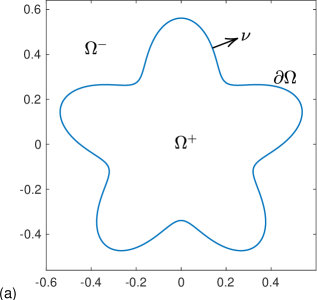
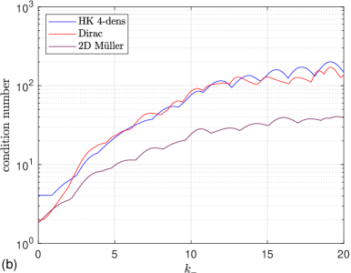
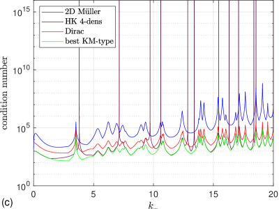
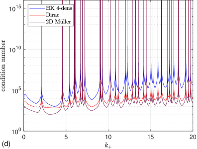
Figure 3. Condition numbers of the operators in “Dirac”, in “HK 4-dens”, in “best KM-type”, and in “2D Müller”: (a) the starfish-like interface $\partial\Omega$; (b) the positive dielectric case; (c) the plasmonic case; (d) the reverse plasmonic case.

9.1. The operators

We compute condition numbers of the discretized system matrices in the systems under study. The main purpose is to detect false eigenwavenumbers. Another purpose is to compare the conditions number of the system matrices with each other. The interface $\partial\Omega$ is the smooth starfish-like curve [22, eq. (92)], shown in Figure 3(a) and originally suggested for scattering problems in [16]. A number of $976$ discretization points are placed on $\partial\Omega$. We study three cases of jumps $\hat{k}$ where we vary $k_{-}$ or $k_{+}$:

• The positive dielectric case. The exterior wavenumber is positive real, $0<k_{-}\leq 20$, and $\hat{k}=k_{+}/k_{-}=1.5$ so that $0<k_{+}\leq 30$ and $\hat{\epsilon}=2.25$. This corresponds to the lower left corner point in Figure 1, where Theorem 2.2 guarantees that no true eigenwavenumbers exist, as well as no false eigenwavenumbers for “Dirac”.

  Figure 3(b) shows that “Dirac” and “HK 4-dens” perform equally well, except at low frequencies where the condition number of “Dirac” fares better and is comparable to that of “2D Müller”.

• The plasmonic case. Again the exterior wavenumber is positive real, $0<k_{-}\leq 20$, but $\hat{k}=k_{+}/k_{-}=i\sqrt{1.1838}$ so that $0<k_{+}/i\leq 20\sqrt{1.1838}$, $k_{+}$ is imaginary, and $\hat{\epsilon}=-1.1838$ is rather close to the essential spectrum $\{-1\}$. This corresponds to the left middle corner point in Figure 1, where Theorem 2.2 guarantees that no true eigenwavenumbers exist, as well as no false eigenwavenumbers for “Dirac”.

  Figure 3(c) shows that the condition number of “Dirac” is closer to that of “best KM-type” than to “HK 4-dens”, in particular at high frequencies. “2D Müller” exhibits $12$ false eigenwavenumbers.

• The reverse plasmonic case. Now the interior wavenumber is positive real, $0<k_{+}\leq 20$, and $\hat{k}=k_{+}/k_{-}=(i\sqrt{1.1838})^{-1}$ so that $0<k_{-}/i\leq 20\sqrt{1.1838}$, $k_{-}$ is imaginary, and $\hat{\epsilon}=-1/1.1838$. This corresponds to the lower middle corner point in Figure 1, which does not belong to the hexagon, and indeed Figure 3(d) shows $37$ true eigenwavenumbers. The different systems here have a relative performance similar to that of the plasmonic case, with “Dirac” performing rather close to “2D Müller”.

9.2. Field computations

We solve the Dirac system (10) for $h$, compute interior and exterior fields $U^{\pm}$ via (12), and compare with results from the other systems. Gradient fields $\nabla U^{\pm}$ are not computed, but we remark that the representation formula (13) for $\nabla U^{\pm}$ uses layer potentials with the same type of (near-logarithmic and near-Cauchy) singular kernels as the representation formula (12). The $2\times 2$ systems, on the other hand, have accompanying representation formulas for $\nabla U^{\pm}$ with layer potentials that contain near-hypersingular kernels. Evaluation of these layer potentials at field points near $\partial\Omega$ may cause additional loss of accuracy.

The curve $\partial\Omega$ is chosen as the boundary of the one-corner drop-like object [22, Eq. (92)], discernible in Figure 4(a). We let $k_{-}=18$ in the positive dielectric and plasmonic cases, and $k_{+}=18$ in the reverse plasmonic case. The incoming wave is a plane wave from south-west, $u^{0}(x,y)=e^{ik_{-}(x+y)/\sqrt{2}}$, and $800$ discretization points are placed on $\partial\Omega$. When $\hat{\epsilon}=-1.1838$, then $\pm(\hat{\epsilon}+1)/(\hat{\epsilon}-1)$ is in the essential $H^{1/2}(\partial\Omega)$-spectrum of (1) and a homotopy-based numerical procedure is adopted where $\hat{\epsilon}=-1.1838$ is approached from above in the complex plane [17, Sec. 6.3].

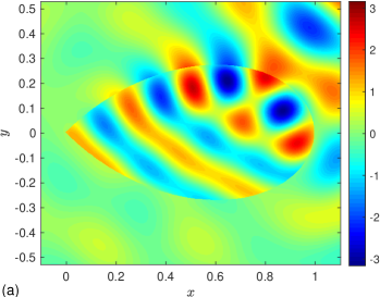
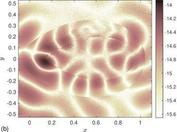
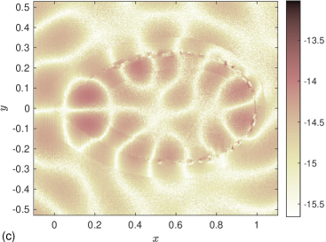
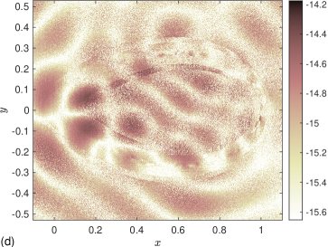
Figure 4. Field computation in the positive dielectric case; (a) the scattered fields $\operatorname{Re}U^{\pm}$; (b) $\log_{10}$ of the estimated absolute error using “HK 4-dens”; (c) same using “Dirac”; (d) same using “2D Müller”.

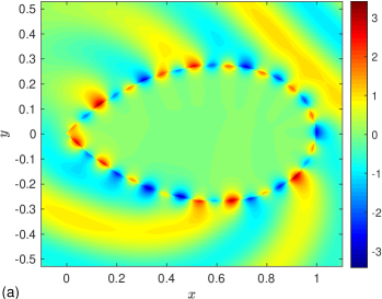
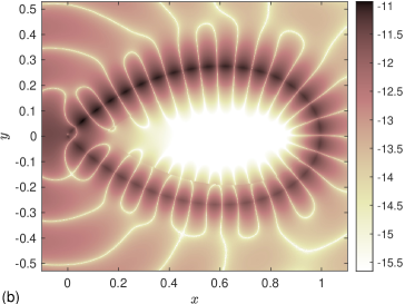
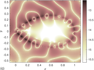
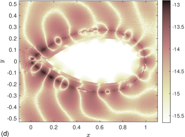
Figure 5. Field computation in the plasmonic case; (a) the scattered fields $\operatorname{Re}U^{\pm}$; (b) $\log_{10}$ of the estimated absolute error using “HK 4-dens”; (c) same using “Dirac”; (d) same using “best KM-type”.

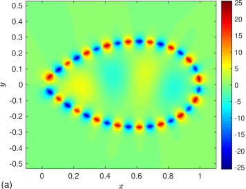
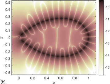
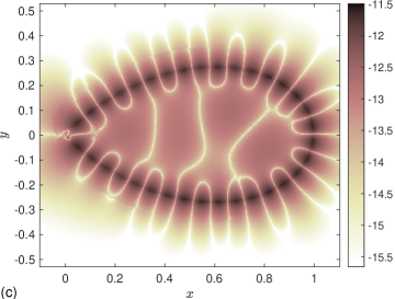
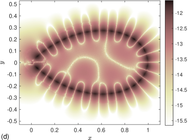
Figure 6. Field computation in the reverse plasmonic case; (a) the scattered fields $\operatorname{Re}U^{\pm}$; (b) $\log_{10}$ of the estimated absolute error using “HK 4-dens”; (c) same using “Dirac”; (d) same using “2D Müller”.

• Figure 4 covers the positive dielectric case. The real parts of the scattered fields $U^{\pm}$ are shown in Figure 4(a). There are propagating waves in both $\Omega^{+}$ and $\Omega^{-}$. The remaining images show $\log_{10}$ of the estimated absolute pointwise error in $\operatorname{Re}U^{\pm}$, computed from the different systems. “Dirac” loses one digit of accuracy in some regions near $\partial\Omega$ compared to the other systems. Most likely, this is because (12) does not exploit null-fields in the near-field evaluation. See [23, Sec. 7].

  The number of GMRES iterations needed to meet a stopping criterion threshold of machine epsilon in the relative residual are $61$, $65$, and $44$ for “HK 4-dens”, “Dirac”, and “2D Müller”, respectively. In this case the operators in “HK 4-dens” and “Dirac” seem to have similar spectral properties, while the spectral properties of the operator in “2D Müller” are better.

• Figure 5 covers the plasmonic case and is organized as Figure 4. There are propagating waves in $\Omega^{-}$, exponentially decaying waves into $\Omega^{+}$, and a surface plasmon wave along $\partial\Omega$. “Dirac” here performs almost on par with “best KM-type” and gives $2$ more accurate digits than “HK 4-dens”.

  The number of GMRES iterations needed are $266$, $173$, and $143$ for “HK 4-dens”, “Dirac”, and “best KM-type”, respectively. In this case the operator in “Dirac” seems to have considerably better spectral properties than the operator in “HK 4-dens”.

• Figure 6 covers the reverse plasmonic case. The results are similar to those of the plasmonic case, although a digit is lost with all systems and we have propagating waves in $\Omega^{+}$ and exponentially decaying waves into $\Omega^{-}$. “Dirac” performs almost on par with “2D Müller” and gives $2$ more accurate digits than than “HK 4-dens”.

9.3. Densities and function spaces

We show asymptotics of the density $h=[h_{1}\;h_{2}\;h_{3}\;h_{4}]^{\rm T}$ obtained from the Dirac integral equation (10). The computations relate to the three examples for the drop-like object in Section 9.2.

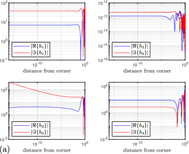
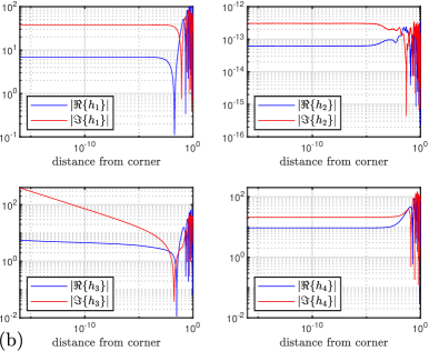
Figure 7. The densities $h_{1},h_{2},h_{3},h_{4}$ as functions of the arc length distance to the corner vertex in the positive dielectric case: (a) along the lower part of $\partial\Omega$; (b) along the upper part of $\partial\Omega$.

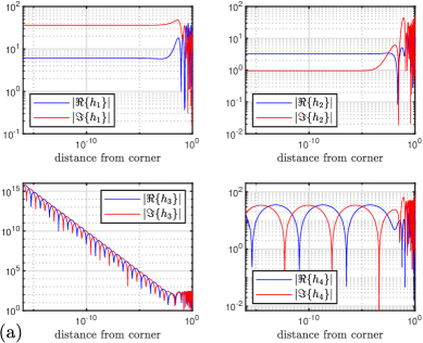
Figure 8. Same as Figure 7, but for the plasmonic case.

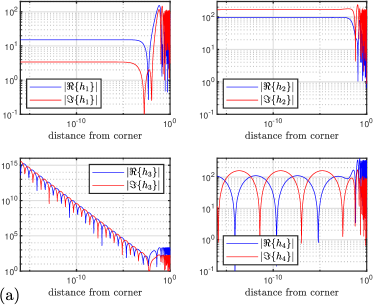
Figure 9. Same as Figure 7, but for the reverse plasmonic case.

• The positive dielectric case: Here the hypothesis on $\hat{\epsilon}$ and $\hat{k}$ in Theorem 2.2 is satisfied. Then $h$ belongs to the energy function space ${\mathcal{H}}_{2}$ from (63), meaning that $h_{1},h_{2}\in H^{1/2}(\partial\Omega)$ and $h_{3},h_{4}\in H^{-1/2}(\partial\Omega)$. The result is shown in Figure 7, where indeed $h_{1}$ and $h_{2}$ are seen to be continuous at the corner vertex (note that $h_{2}\approx 0$). The only singular density is $h_{3}$, which is related to that it is only the $(3,3)$ diagonal element in the $4\times 4$ block-operator of (10) which we do not control by the choices of parameters $r,\beta,\alpha^{\prime},\beta^{\prime}$ in Section 7. Using the automated eigenvalue method of [18, Sec. 14], the asymptotic behaviour of $h_{3}$ near the corner is determined to be

  (136) $$h_{3}(t)\propto t^{\eta},$$

  where $\eta=-0.12319432456634$ and $t$ is the arc length distance to the corner vertex. So $h_{3}$ is in fact in $L_{2}(\partial\Omega)$.

• The plasmonic case: Here the hypothesis on $\hat{\epsilon}$ and $\hat{k}$ in Theorem 2.2 is not satisfied since $\hat{\epsilon}<0$ makes $\pm(\hat{\epsilon}+1)/(\hat{\epsilon}-1)$ hit the essential $H^{-1/2}(\partial\Omega)$-spectrum of (1). Nevertheless, the RCIP-accelerated Nyström scheme manages to produce the limit solution $h$ shown in Figure 8. As in the positive dielectric case, the densities $h_{1},h_{2},h_{4}$ are good, although $h_{4}$ exhibits an oscillatory behaviour. However $h_{3}\notin H^{-1/2}(\partial\Omega)$. More precisely, its asymptotics near the corner are as in (136) with $\eta=-1.00000000000000-i1.57105873276994$. So $h_{3}\in H^{-s}(\partial\Omega)$ for any $s>1/2$.

• The reverse plasmonic case: the results, shown in Figure 9, are very similar to those of the plasmonic case. The asymptotics of $h_{3}$ are as in (136) with $\eta=-1.00000000000000+i1.57105873276994$.

We end with a remark on the densities $h$ obtained in the plasmonic and reverse plasmonic cases, which fall outside the energy trace space ${\mathcal{H}}_{2}$ from (63). More generally, this energy trace space belongs to a family of function spaces, where Sobolev regularity $s=1/2$ and $s-1=-1/2$ is replaced by a more general regularity index $s$. On Lipschitz domains, the possible range is $0\leq s\leq 1$. In the plasmonic cases, our computed densities $h$ belong to the larger spaces $s<1/2$. For $0\leq s<1$, the corresponding norms of the fields are weighted Sobolev norms using $\int|\nabla U^{\pm}(x)|^{2}\text{dist}(x)^{1-2s}dx$, where $\text{dist}(x)$ denotes distance from $x$ to $\partial\Omega$, whereas for the endpoint $s=1$, this must be replaced by a norm involving a non-tangential maximal function. A reference for the elementary results for $0<s<1$ is Costabel [12]. The bounds on double layer potential operators for the endpoints $s=0,1$ require harmonic analysis and the Coifman–McIntosh–Meyer theorem [10].

The essential spectrum of the double layer potential operator (1) depends on the choice of function space, that is on $s$. For the energy trace space $s=1/2$ this spectrum is a subset of the real interval $(-1,1)$, but in the endpoint spaces $s=0,1$, as alluded to in the introduction, this spectrum can be computed to be a lying “figure eight”, parametrized as

(137) $$\pm\sin(\delta\pi(1+i\xi)/2)/\sin(\pi(1+i\xi)/2),\qquad\xi\in{\mathbf{R}},$$

where $\delta=\theta/\pi-1$ on a domain with a corner of opening angle $\theta$.

The point of departure for the investigations reported on in this paper was the spin integral equation proposed in [36, Sec. 5] for solving the Maxwell transmission problem (14). However, it was soon realized that this was not suitable for the plasmonic and reverse plasmonic cases. Indeed, the theory developed for this spin integral equation makes use of non-diagonal matrices $P,P^{\prime},N,N^{\prime}$ in (10) which mix $H^{\pm 1/2}(\partial\Omega)$ and is limited to the function space $L_{2}(\partial\Omega)^{4}$, which is different from ${\mathcal{H}}_{2}$. As we have seen, surface plasmon waves appear in the function space ${\mathcal{H}}_{2}$ or, in the case of pure meta materials, in the larger function spaces $s<1/2$. The numerical algorithm used here fails for the spin integral equation when the “figure eight” of (137) is approached. When $\hat{\epsilon}=-1.1838$ is approached from above in the complex plane, this happens near $\hat{\epsilon}=-1.1838+i0.2168$.

References

[1]Axelsson, A.Oblique and normal transmission problems for Dirac operators with
strongly Lipschitz interfaces.
Comm. Partial Differential Equations 28, 11-12 (2003),
1911–1941.
[2]Axelsson, A.Transmission problems for Dirac’s and Maxwell’s equations
with Lipschitz interfaces.PhD thesis, The Australian National University, 2003.
Available at
https://openresearch-repository.anu.edu.au/handle/1885/46056.
[3]Axelsson, A.Transmission problems and boundary operator algebras.
Integral Equations Operator Theory 50, 2 (2004), 147–164.
[4]Axelsson, A.Transmission problems for Maxwell’s equations with weakly
Lipschitz interfaces.
Math. Methods Appl. Sci. 29, 6 (2006), 665–714.
[5]Axelsson, A., Grognard, R., Hogan, J., and McIntosh, A.Harmonic analysis of Dirac operators on Lipschitz domains.
In Clifford analysis and its applications (Prague, 2000),
vol. 25 of NATO Sci. Ser. II Math. Phys. Chem. Kluwer Acad. Publ.,
Dordrecht, 2001, pp. 231–246.
[6]Axelsson, A., and McIntosh, A.Hodge decompositions on weakly Lipschitz domains.
In Advances in analysis and geometry, Trends Math.
Birkhäuser, Basel, 2004, pp. 3–29.
[7]Buffa, A., and Ciarlet, P., J.On traces for functional spaces related to Maxwell’s equations.
I. An integration by parts formula in Lipschitz polyhedra.
Math. Methods Appl. Sci. 24, 1 (2001), 9–30.
[8]Buffa, A., and Ciarlet, P., J.On traces for functional spaces related to Maxwell’s equations.
II. Hodge decompositions on the boundary of Lipschitz polyhedra and
applications.
Math. Methods Appl. Sci. 24, 1 (2001), 31–48.
[9]Buffa, A., Costabel, M., and Sheen, D.On traces for in Lipschitz domains.
J. Math. Anal. Appl. 276, 2 (2002), 845–867.
[10]Coifman, R. R., McIntosh, A., and Meyer, Y.L’intégrale de Cauchy définit un opérateur borné sur
pour les courbes lipschitziennes.
Ann. of Math. (2) 116, 2 (1982), 361–387.
[11]Colton, D., and Kress, R.Integral equation methods in scattering theory, first ed.
John Wiley & Sons, New York, 1983.
[12]Costabel, M.Boundary integral operators on Lipschitz domains: elementary
results.
SIAM J. Math. Anal. 19, 3 (1988), 613–626.
[13]Epstein, C., Greengard, L., and O’Neil, M.A high-order wideband direct solver for electromagnetic scattering
from bodies of revolution.
J. Comput. Phys. 387 (2019), 205–229.
[14]Fabes, E., Jodeit, M., and Lewis, J.Double layer potentials for domains with corners and edges.
Indiana Univ. Math. 26, 1 (1977), 95–114.
[15]Ganesh, M., Hawkins, S. C., and Volkov, D.An all-frequency weakly-singular surface integral equation for
electromagnetism in dielectric media: reformulation and well-posedness
analysis.
J. Math. Anal. Appl. 412, 1 (2014), 277–300.
[16]Hao, S., Barnett, A. H., Martinsson, P. G., and Young, P.High-order accurate methods for Nyström discretization of
integral equations on smooth curves in the plane.
Adv. Comput. Math. 40, 1 (2014), 245–272.
[17]Helsing, J.The effective conductivity of arrays of squares: Large random unit
cells and extreme contrast ratios.
J. Comput. Phys. 230, 20 (2011), 7533–7547.
[18]Helsing, J.Solving integral equations on piecewise smooth boundaries using the
RCIP method: a tutorial.
arXiv e-prints, arXiv:1207.6737v9 [physics.comp-ph] (revised 2018).
[19]Helsing, J., and Holst, A.Variants of an explicit kernel-split panel-based Nyström
discretization scheme for Helmholtz boundary value problems.
Adv. Comput. Math. 41, 3 (2015), 691–708.
[20]Helsing, J., and Karlsson, A.Determination of normalized electric eigenfields in microwave
cavities with sharp edges.
J. Comput. Phys. 304 (2016), 465–486.
[21]Helsing, J., and Karlsson, A.Resonances in axially symmetric dielectric objects.
IEEE Trans. Microw. Theory Tech. 65, 7 (2017), 2214–2227.
[22]Helsing, J., and Karlsson, A.On a Helmholtz transmission problem in planar domains with corners.
J. Comput. Phys. 371 (2018), 315–332.
[23]Helsing, J., and Karlsson, A.An extended charge-current formulation of the electromagnetic
transmission problem.
SIAM J. Appl. Math. 80, 2 (2020), 951–976.
[24]Helsing, J., Karlsson, A., and Rosén, A.Comparison of integral equations for the Maxwell transmission
problem with general permittivities.
arXiv e-prints, arXiv:2007.12260 [physics.comp-ph].
[25]Helsing, J., and Perfekt, K.-M.The spectra of harmonic layer potential operators on domains with
rotationally symmetric conical points.
J. Math. Pures Appl. 118 (2018), 235–287.
[26]Hernández-Herrera, A.Higher dimensional transmission problems for Dirac operators on
Lipschitz domains.
J. Math. Anal. Appl. 478, 2 (2019), 499–525.
[27]Kleinman, R., and Martin, P.On single integral equations for the transmission problem of
acoustics.
SIAM J. Appl. Math. 48, 2 (1988), 307–325.
[28]Kress, R., and Roach, G.Transmission problems for the Helmholtz equation.
J. Math. Phys. 19, 6 (1978), 1433–1437.
[29]Lai, J., and O’Neil, M.An FFT-accelerated direct solver for electromagnetic scattering
from penetrable axisymmetric objects.
J. Comput. Phys. 390 (2019), 152–174.
[30]Marmolejo-Olea, E., Mitrea, I., Mitrea, M., and Shi, Q.Transmission boundary problems for Dirac operators on Lipschitz
domains and applications to Maxwell’s and Helmholtz’s equations.
Trans. Amer. Math. Soc. 364, 8 (2012), 4369–4424.
[31]McIntosh, A., and Mitrea, M.Clifford algebras and Maxwell’s equations in Lipschitz domains.
Math. Methods Appl. Sci. 22, 18 (1999), 1599–1620.
[32]Müller, C.Foundations of the mathematical theory of electromagnetic
waves.
Revised and enlarged translation from the German. Die Grundlehren der
mathematischen Wissenschaften, Band 155. Springer-Verlag, Berlin, 1969.
[33]Picard, R.On the low frequency asymptotics in electromagnetic theory.
J. Reine Angew. Math. 354 (1984), 50–73.
[34]Picard, R.On a structural observation in generalized electromagnetic theory.
J. Math. Anal. Appl. 110, 1 (1985), 247–264.
[35]Rosén, A.A spin integral equation for electromagnetic and acoustic scattering.
Appl. Anal. 96, 13 (2017), 2250–2266.
[36]Rosén, A.Boosting the Maxwell double layer potential using a right spin
factor.
Integral Equations Operator Theory 91, 3 (2019), Paper No. 29,
25.
[38]Schultz, E., and Hiptmair, R.First-kind boundary integral equations for the Dirac operator in
3D Lipschitz domains.
arXiv e-prints, arXiv:2012.11994 [math.AP].
[39]Taskinen, M., and Vänskä, S.Current and charge integral equation formulations and Picard’s
extended Maxwell system.
IEEE Trans. Antennas and Propagation 55, 12 (2007), 3495–3503.
[40]Taskinen, M., and Ylä-Oijala, P.Current and charge integral equation formulation.
IEEE Trans. Antennas and Propagation 54, 1 (2006), 58–67.
[41]Vico, F., Greengard, L., and Ferrando, M.Decoupled field integral equations for electromagnetic scattering
from homogeneous penetrable obstacles.
Comm. Part. Differ. Equat. 43, 2 (2018), 159–184.
[42]Weck, N.Traces of differential forms on Lipschitz boundaries.
Analysis (Munich) 24, 2 (2004), 147–169.