Adaptive Statistical Learning with Bayesian Differential Privacy

Abstract.

In statistical learning, a dataset is often partitioned into two parts: the training set and the holdout (i.e., testing) set. For instance, the training set is used to learn a predictor, and then the holdout set is used for estimating the accuracy of the predictor on the true distribution. However, often in practice, the holdout dataset is reused and the estimates tested on the holdout dataset are chosen adaptively based on the results of prior estimates, leading to that the predictor may become dependent of the holdout set. Hence, overfitting may occur, and the learned models may not generalize well to the unseen datasets. Prior studies have established connections between the stability of a learning algorithm and its ability to generalize, but the traditional generalization is not robust to adaptive composition. Recently, Dwork et al. in NIPS, STOC, and Science 2015 show that the holdout dataset from i.i.d. data samples can be reused in adaptive statistical learning, if the estimates are perturbed and coordinated using techniques developed for differential privacy, which is a widely used notion to quantify privacy. Yet, the results of Dwork et al. are applicable to only the case of i.i.d. samples. In contrast, correlations between data samples exist because of various behavioral, social, and genetic relationships between users. Our results in adaptive statistical learning generalize the results of Dwork et al. for i.i.d. data samples to arbitrarily correlated data. Specifically, we show that the holdout dataset from correlated samples can be reused in adaptive statistical learning, if the estimates are perturbed and coordinated using techniques developed for Bayesian differential privacy, which is a privacy notion recently introduced by Yang et al. in SIGMOD 2015 to broaden the application scenarios of differential privacy when data records are correlated.

1. Introduction

In many statistical learning algorithms, a common practice is to partition a dataset into two parts: the training set and the holdout (i.e., testing) set. For instance, after the training set is used to learn a predictor, the holdout set is used for estimating the accuracy of the predictor on the true distribution. However, in many practical applications, since (i) the holdout dataset is reused, and (ii) the estimates tested on the holdout dataset are chosen adaptively based on the results of prior estimates, we observe that the predictor may become dependent of the holdout set. This leads to the result that overfitting may occur, and the learned models may not generalize well to the unseen datasets. Several papers (Bousquet and Elisseeff, 2002; Mukherjee et al., 2006; Poggio et al., 2004; Shalev-Shwartz et al., 2010) in the literature have established connections between the stability of a learning algorithm and its ability to generalize, but the traditional generalization is not robust to adaptive composition (Bassily and Freund, 2016; Cummings et al., 2016; Dwork et al., 2015b). To remedy this issue, Dwork et al. (Dwork et al., 2015a, b, c) recently show that the holdout dataset from i.i.d. data samples can be reused in adaptive statistical learning, if the estimates are perturbed and coordinated using techniques developed for differential privacy, which has emerged as the standard notion to quantify privacy and will be elaborated next.

Differential privacy by Dwork et al. (Dwork, 2006; Dwork et al., 2006b) is a privacy notion that has been successfully applied to a range of statistical learning tasks, since it offers a rigorous foundation for defining privacy. Differential privacy has received considerable interest in the literature (Blocki et al., 2016; Xiao and Xiong, 2015; Zhang et al., 2016; Lou et al., 2017; Wang et al., 2017; Shokri and Shmatikov, 2015). The Chrome browser by Google has used a differentially private tool called RAPPOR (Erlingsson et al., 2014) to collect information about clients. Starting from iOS 10, Apple (Apple Incorporated, 2016) has incorporated differential privacy into its mobile operating system. A randomized mechanism $Y$ satisfies $\epsilon$-differential privacy if for all neighboring databases $x$ and $x^{\prime}$ that differ in one record, and for any subset $\mathcal{Y}$ of the output range of the mechanism $Y$, it holds that $\mathbb{P}[Y(x)\in\mathcal{Y}]\leq e^{\epsilon}\mathbb{P}[Y(x^{\prime})\in\mathcal{Y}],$ where $\mathbb{P}[\cdot]$ denotes the probability and $e$ is a mathematical constant that is the base of the natural logarithm. Intuitively, under differential privacy, an adversary given access to the output does not have much confidence to determine whether the output was sampled from the probability distribution generated by the randomized algorithm when the database is $x$ or when the database is $x^{\prime}$ that is different from $x$ by one record.

Dwork et al. (Dwork et al., 2015a, b, c) show that the holdout dataset from i.i.d. data samples can be reused in adaptive statistical learning, if the estimates are perturbed and coordinated using algorithms satisfying differential privacy. These efforts by Dwork et al. (Dwork et al., 2015a, b, c) have attracted significant attention to adaptive statistical learning (Bassily and Freund, 2016; Blum and Hardt, 2015; Cummings et al., 2016; Rogers et al., 2016; Russo and Zou, 2016). However, existing studies for adaptive statistical learning including those of Dwork et al. (Dwork et al., 2015a, b, c) are applicable to only the case of i.i.d. samples. In contrast, correlations between data samples exist because of various behavioral, social, and genetic relationships between users (Zhao et al., 2017). In location privacy, a user’s locations across time exhibit temporal correlations (Olteanu et al., 2017; Xiao and Xiong, 2015; Song et al., 2017), and locations of friends tend to have social correlations since they are likely to visit the same place (Liu et al., 2016; Backstrom et al., 2010). In genome privacy, DNA information is passed from parents to children based on Mendelian inheritance so family members’ genotypes are correlated, where a genotype is the set of genes in DNA responsible for a particular trait (Humbert et al., 2013). In short, real-world data samples may contain a rich set of correlations.

Our results in adaptive statistical learning generalize recent work of Dwork et al. (Dwork et al., 2015a, b, c) for i.i.d. data samples to arbitrarily correlated data. In other words, we tackle adaptive statistical learning with correlated data samples while Dwork et al. (Dwork et al., 2015a, b, c) consider only i.i.d. samples. Specifically, we show that the holdout dataset from correlated samples can be reused in adaptive statistical learning, if the estimates are perturbed and coordinated using techniques developed for Bayesian differential privacy, a privacy notion recently introduced by Yang et al. (Yang et al., 2015) to address correlations in a database. It has been observed by Kifer and Machanavajjhala (Kifer and Machanavajjhala, 2011) (see also (Chen et al., 2014; He et al., 2014; Kifer and Machanavajjhala, 2012; Liu et al., 2016; Song et al., 2017; Zhu et al., 2015; Zhao et al., 2017)) that differential privacy may not work as expected when the data tuples are correlated. The underlying reason according to Zhao et al. (Zhao et al., 2017) is that differential privacy’s guarantee masks only the presence of those records received from each user, but could not mask statistical trends that may reveal information about each user. Bayesian differential privacy (Yang et al., 2015) broadens the application scenarios of differential privacy when data records are correlated. For clarity, we defer the detailed definition of Bayesian differential privacy to Section 2.3.

The rest of the paper is organized as follows. We discuss some preliminaries in Section 2, before presenting our results of adaptive statistical learning in Section 3. Section 4 provides experiments to support our results. We elaborate the proofs in Section 5. Section 6 surveys related work, and Section 7 concludes the paper.

2. Preliminaries

2.1. Adaptive Statistical Learning

Dwork et al. (Dwork et al., 2015a) show that differential privacy techniques can be leveraged in adaptive statistical learning for i.i.d. data samples. To this end, they introduce the notion of approximate max-information, establish a connection of differential privacy to approximate max-information, and utilize this connection to present an algorithm for adaptive statistical learning.

For two random variables $X$ and $Y$, let $X\times Y$ be the random variable obtained by drawing $X$ and $Y$ independently from their probability distributions, and let $\textrm{domain}(X,Y)$ be the domain of $(X,Y)$. Dwork et al. (Dwork et al., 2015a) define the notion of $\beta$-approximate max-information as follows:

(1) $$I_{\infty}^{\beta}(X;Y)\stackrel{{\scriptstyle\text{def}}}{{=}}\log\max\limits_{\begin{subarray}{l}\mathcal{O}\subseteq\textrm{domain}(X,Y):\\ {\mathbb{P}}\left[{(X,Y)\in\mathcal{O}}\right]>\beta\end{subarray}}\frac{{\mathbb{P}}\left[{(X,Y)\in\mathcal{O}}\right]-\beta}{{\mathbb{P}}\left[{X\times Y\in\mathcal{O}}\right]},$$

where $\beta>0$ and $\log$ means the binary logarithm. Approximate max-information gives generalization since it upper bounds the probability of “bad events” that can occur as a result of the dependence of the learning result $Y(X)$ on the dataset $X$; see  (Dwork et al., 2015a, Page 10) for more details. Specifically, it is straightforward to obtain from (1) that if

$$I_{\infty}^{\beta}(X;Y(X))=k,$$

then

$${\mathbb{P}}\left[{(X,Y)\in\mathcal{O}}\right]\leq 2^{k}\cdot{\mathbb{P}}\left[{X\times Y\in\mathcal{O}}\right]+\beta$$

for any $\mathcal{O}\subseteq\textrm{domain}(X,Y)$.

Statistical learning considered in this paper is as follows: For an unknown distribution $\mathcal{D}$ over a discrete universe $\mathcal{X}$ of possible data points, a statistical query $Q$ asks for the expected value of some function $f:\mathcal{X}\rightarrow[0,1]$ on random draws from $\mathcal{D}$. The goal is to ensure that the estimate obtained from data is close to the true result on the unknown distribution. We consider queries $Q_{1},Q_{2},\ldots$ that are chosen adaptively based on the results of prior estimates.

2.2. Differential Privacy

A randomized algorithm $Y$ satisfies $\epsilon$-differential privacy (DP) if for all neighboring databases $x$ and $x^{\prime}$ that differ in one record, and for any subset $\mathcal{Y}$ of the output range of the mechanism $Y$, it holds that

(2) $$\mathbb{P}[Y(x)\in\mathcal{Y}]\leq e^{\epsilon}\mathbb{P}[Y(x^{\prime})\in\mathcal{Y}].$$

To ensure $\epsilon$-differential privacy, the Laplace mechanism (Dwork et al., 2006b) and the exponential mechanism (McSherry and Talwar, 2007) have been proposed in the literature. The details are as follows.

• To achieve $\epsilon$-differential privacy for a query $Q$, the Laplace mechanism $\text{Lap}({\Delta_{Q}}/{\epsilon})$ adds Laplace noise with parameter (i.e., scale) ${\Delta_{Q}}/{\epsilon}$ independently to each dimension of the query result, where $\Delta_{Q}$ is the global sensitivity of query $Q$:
  $\Delta_{Q}=\max_{\textrm{neighboring $x,x^{\prime}$}}\|Q(x)-Q(x^{\prime})\|_{1}$, where databases $x$ and $x^{\prime}$ are neighboring if they differ in one record.

• To ensure $\epsilon$-differential privacy for a query $Q$, the exponential mechanism $\text{Expo}(\epsilon,u,\mathcal{R})$ for some utility function $u$ and the output range $\mathcal{R}$ outputs an element $y\in\mathcal{R}$ with probability proportional to $\exp\big{(}\frac{\epsilon\cdot u(x,y)}{2\Delta_{u}}\big{)}$, where $\Delta_{u}$ is the sensitivity of $u$ with respect to its database argument:
  $\Delta_{u}=\max_{y\in\mathcal{R}}\max_{\textrm{neighboring $x,x^{\prime}$}}|u(x,y)-u(x^{\prime},y)|$, where data- bases $x$ and $x^{\prime}$ are neighboring if they differ in one record.

Although differential privacy (DP) has been recognized as a powerful notion, it has been observed by Kifer and Machanavajjhala (Kifer and Machanavajjhala, 2011) (see also (Chen et al., 2014; He et al., 2014; Kifer and Machanavajjhala, 2012; Liu et al., 2016; Song et al., 2017; Zhu et al., 2015; Zhao et al., 2017)) that DP may not work as expected when the data tuples are correlated. As noted by Zhao et al. (Zhao et al., 2017), although DP ensures that a user’s participation itself in the computation reveals no further secrets from the user, however, due to tuple correlation, a user’s data may impact other users’ records and hence has more influence on the query response than what is expected compared with the case where tuples are independent. When correlations exist, a user’s data is not known to the user alone in some degree, and an adversary may combine the query output and the correlation to learn about a user’s data.

To extend differential privacy for correlated data, prior studies have investigated various privacy metrics (Chen et al., 2014; He et al., 2014; Kifer and Machanavajjhala, 2012; Liu et al., 2016; Song et al., 2017; Zhu et al., 2015). One of the metrics receiving much attention is the notion of Bayesian differential privacy introduced by Yang et al. (Yang et al., 2015) as follows.

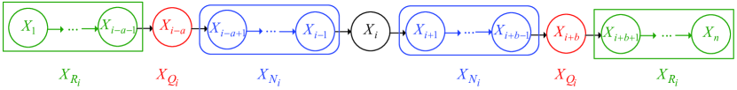
Figure 1. This figure from (Zhao et al., 2017) is based on (Song et al., 2017). For a Markov chain $X_{1}\to X_{2}\ldots\to X_{n}$, moralization simply means making each directed edge undirected, since there are no nodes that have a common child. A Markov quilt for node $X_{i}$ is $X_{Q_{i}}=\{X_{i-a},X_{i+b}\}$. The corresponding nearby set $X_{N_{i}}$ and remote set $X_{R_{i}}$ are $X_{N_{i}}=\{X_{i-a+1},\ldots,X_{i-1}\}\hskip 2.0pt{\cup}\hskip 2.0pt\{X_{i+1},\ldots,X_{i+b-1}\}$ and $X_{R_{i}}=\{X_{1},\ldots,X_{i-a-1}\}\hskip 2.0pt{\cup}\hskip 2.0pt\{X_{i+b+1},\ldots,X_{n}\}$. To check the definition of a Markov quilt, it is straightforward to see that here any path between $X_{i}$ and a node in $X_{R_{i}}$ has to include at least one node in $X_{Q_{i}}$. Both $a$ and $b$ above are positive integers. If $a=1$ and $b=1$, the Markov quilt becomes the Markov blanket $X_{M_{i}}=\{X_{i-1},X_{i+1}\}$ with the corresponding $X_{N_{i}}$ being $\emptyset$. Note that any $X$ term with an index outside of $\{1,2,\ldots,n\}$ is canceled out; e.g., the Markov blanket $X_{M_{1}}$ of node $X_{1}$ is actually $\{X_{2}\}$ rather than $\{X_{0},X_{2}\}$ since there is no node $X_{0}$.

2.3. Bayesian Differential Privacy

In this paper, we will establish a connection of Bayesian differential privacy to approximate max-information and then leverage this connection to use Bayesian differential privacy for adaptive statistical learning. We discuss Bayesian differential privacy below.

The notion of Bayesian differential privacy (BDP) is introduced by Yang et al. (Yang et al., 2015) to extend differential privacy for addressing the case when data records are correlated. Before stating the definition, we first introduce some notation.

The database under consideration is modeled by a random variable $X=[{X}_{1},{X}_{2},\ldots,{X}_{n}]$, where ${X}_{j}$ for each $j\in\{1,\ldots,n\}$ is a tuple, which is also a random variable. Let database $x=[x_{1},x_{2},\ldots,x_{n}]$ be an instantiation of $X$, so that each ${x}_{j}$ denotes an instantiation of ${X}_{j}$. Let $i$ be the index of the tuple attacked by the adversary. For notational simplicity, $x_{S}$ and $X_{S}$ stand for $[x_{j}:j\in S]$ and $[X_{j}:j\in S]$ respectively for any set $S\subseteq\{1,2,\ldots,n\}\setminus\{i\}$; i.e., $x_{S}$ is an instantiation of ${X}_{S}$. An adversary denoted by $A(i,S)$ knows the values of all tuples in $S$ (denoted by $x_{S}$) and attempts to attack the value of tuple $i$ (denoted by $x_{i}$). For a randomized perturbation mechanism $Y$ that maps a database $x$ to a randomized output $y$, the Bayesian differential privacy leakage (BDPL) of $Y$ with respect to the adversary $A(i,S)$ is defined by

(3) $$\text{BDPL}_{A}(Y)=\text{sup}_{x_{i},x_{i}^{\prime},x_{S},\mathcal{Y}}\ln\frac{\mathbb{P}[y\in\mathcal{Y}\boldsymbol{\mid}x_{i},x_{S}]}{\mathbb{P}[y\in\mathcal{Y}\boldsymbol{\mid}x_{i}^{\prime},x_{S}]},$$

where the subscript $A$ is short for $A(i,S)$, and $\ln$ denotes the natural logarithm. In (3), $x_{i}$ and $x_{i}^{\prime}$ iterate through the domain of tuple $X_{i}$ (i.e., $x_{i}\in\textrm{domain}(X_{i})$, $x_{i}^{\prime}\in\textrm{domain}(X_{i})$, and $x_{i}\neq x_{i}^{\prime}$), and $x_{S}$ iterates through the domain of tuple(s) $X_{S}$ (i.e., $x_{S}\in\textrm{domain}(X_{S})$), where $X_{S}$ and $x_{S}$ stand for $[X_{j}:j\in S]$ and $[x_{j}:j\in S]$ respectively for $S\subseteq\{1,2,\ldots,n\}\setminus\{i\}$. In (3), $\mathcal{Y}$ iterates through all subsets of the output range of the mechanism $Y$.

The mechanism $Y$ satisfies $\epsilon$-Bayesian differential privacy if

(4) $$\text{sup}_{A}\text{BDPL}_{A}(Y)\leq\epsilon.$$

In (4), $A$ (short for $A(i,S)$) iterates through the set of all adversaries; i.e., $i$ iterates through the index set $\{1,\ldots,n\}$ and $S$ iterates through all subsets of $\{1,2,\ldots,n\}\setminus\{i\}$.

Based on (2)–(4), Yang et al. (Yang et al., 2015) show that when all tuples are independent, (2) (i.e., DP guarantee) and (4) (i.e., BDP guarantee) are the same. However, under tuple correlations, (2) (i.e., DP guarantee) and (4) (i.e., BDP guarantee) are different due to the following reason (Zhao et al., 2017): although DP protects the information received from each user, an adversary may combine the correlations and the query response to obtain a large amount of information about the user. In other words, under DP, although the user itself is privacy-aware in participating the database, the participations of other users together with the query response nevertheless leak the user’s data. The BDP notion ensures that even under tuple correlation, almost no sensitive information about any user can be leaked because of answering the query.

2.4. Mechanisms to Achieve Bayesian Differential Privacy

Yang et al. (Yang et al., 2015) extend the Laplace mechanism (Dwork et al., 2006b) of differential privacy to achieve Bayesian differential privacy. However, this mechanism of (Yang et al., 2015) is only for the sum query on a Gaussian Markov random field (GMRF) with positive correlations and its extension to a discrete domain, so it cannot apply to queries other than the sum query and cannot apply to correlations other than those of positive-correlated GMRF. Recently, my co-authors and I (Zhao et al., 2017) present mechanisms for arbitrary correlations by connecting Bayesian differential privacy (BDP) to differential privacy (DP). Specifically, we (Zhao et al., 2017) show that $\epsilon^{\prime}$-DP implies $\epsilon$-BDP, where $\epsilon^{\prime}$ depends on $\epsilon$ and the correlations between the data tuples. Note that although (Zhao et al., 2017) uses the notion of dependent differential privacy, this notion is equivalent to Bayesian differential privacy.

For clarity, we will present (Zhao et al., 2017)’s results on the relationship between Bayesian differential privacy (BDP) and differential privacy (DP) as Lemmas 2–4 in Section 5.1 later. In order to state these results as well as our main results on adaptive statistical learning in Section 3, we first review some preliminaries given in (Zhao et al., 2017).

Representing dependency structure of tuples of a database via probability graphical models. To represent dependency structure of tuples in a database, we (Zhao et al., 2017) apply the well-known notion called probability graphical model. These models use graphs (i.e., networks) to express the conditional (in)dependencies between random variables. In our applications, each node stands for a tuple of the database (a tuple is also a random variable), and we have a network to represent the conditional (in)dependencies between tuples of the database.

A Bayesian network (which is a directed acyclic graph) and a Markov network (which is an undirected graph) are two kinds of probability graphical models that have been studied extensively and used in various applications (Koller and Friedman, 2009). A Bayesian network is a directed acyclic graph which represents a factorization of the joint probability of all random variables. Specifically, in a Bayesian network of $n$ nodes $\{X_{1},X_{2},\ldots,X_{n}\}$, with $\textrm{{PA}}_{i}$ denoting the set of parents of node $X_{i}$ (i.e., each node of $\textrm{{PA}}_{i}$ points directly to node $X_{i}$ via a single directed edge), then the joint probability satisfies ${\mathbb{P}}\left[{X_{1},X_{2},\ldots,X_{n}}\right]=\prod_{i=1}^{n}{\mathbb{P}}\left[{X_{i}\boldsymbol{\mid}\textrm{{PA}}_{i}}\right]$. A Markov network represents (in)dependencies between random variables via an undirected graph which has the Markov property such that any two subsets of variables are conditionally independent given a separating subset; i.e., with $A,B,C$ denoting three disjoint sets of nodes, if any path between any node $a\in A$ and any node $b\in B$ has to include at least one node in $C$ (or there is simply no path between $a\in A$ and $b\in B$), then $A$ and $B$ are conditionally independent given $C$.

Markov blanket. The notion of Markov blanket is standard in probability graphical models (Koller and Friedman, 2009). For a node $X_{i}$, its Markov blanket $X_{M_{i}}$ comprises the tuples that are directly correlated with tuple $X_{i}$ (i.e., given $X_{M_{i}}$ which contains $X_{j}$ for $j\in M_{i}$, $X_{i}$ is conditionally independent of everything else). If $X_{i}$ is independent of all other $n-1$ tuples, then $M_{i}=\emptyset$. In a Bayesian network, a node’s Markov blanket consists of its parents, children, and its children’s other parents. In a Markov network (also known as a Markov random field), the Markov blanket of a node is its set of neighboring nodes.

Markov quilt. We (Zhao et al., 2017) generalize the notion of Markov blanket to Markov quilt. This definition is adopted from Song et al. (Song et al., 2017) with slight changes. We consider a network of $n$ nodes $X_{1},X_{2},\ldots,X_{n}$. First, we perform moralization if necessary. In other words, for a Bayesian network, we moralize it into a Markov network; for a Markov network, no action is taken. Moralization means making each directed edge undirected and putting an edge between any two nodes that have a common child. Recall that $X_{S}$ represents the set of nodes with indicies in an index set $S$, where $S\subseteq\{1,2,\ldots,n\}$; i.e. $X_{S}=\{X_{j}:j\in S\}$. Let $Q_{i}$ and $R_{i}$ be disjoint subsets of $\{1,2,\ldots,n\}\setminus\{i\}$. We say a set $X_{Q_{i}}$ of nodes is a Markov quilt of node $X_{i}$ if after moralization (whenever necessary) of the dependency network, for any node $X_{j}$ in $X_{R_{i}}$, either any path between $X_{i}$ and $X_{j}$ has to include at least one node in $X_{Q_{i}}$, or there is simply no path between $X_{i}$ and $X_{j}$. We emphasize that this definition is defined on a Markov network or after we have moralized a Bayesian network into a Markov network. The definition implies that $X_{R_{i}}$ is independent of $X_{i}$ conditioning on $X_{Q_{i}}$. Excluding $X_{i}$, $X_{Q_{i}}$ and $X_{R_{i}}$, we define the remaining nodes as $X_{N_{i}}$; i.e., $X_{Q_{i}}$, $X_{N_{i}}$, $X_{R_{i}}$ together constitute a partition of $\Big{\{}X_{j}:j\in\{1,2,\ldots,n\}\setminus\{i\}\Big{\}}$ so that $Q_{i},R_{i},N_{i}$ together partition $\{1,2,\ldots,n\}\setminus\{i\}$. Intuitively, $X_{Q_{i}}$ separates $X_{i}$ and $X_{R_{i}}$, so $X_{R_{i}}$ is remote from $X_{i}$ while $X_{N_{i}}$ is nearby from $X_{i}$ (this is why we use the notation $R$ and $N$). We refer to $X_{N_{i}}$ (resp., $X_{R_{i}}$) as the nearby set (resp., the remote set) associated with the Markov quilt $X_{Q_{i}}$. Note that when we define a Markov quilt $X_{Q_{i}}$ for node $X_{i}$, we actually have a triple $(X_{Q_{i}},X_{N_{i}},X_{R_{i}})$: a Markov quilt $X_{Q_{i}}$, a nearby set $X_{N_{i}}$, and a remote set $X_{R_{i}}$. Figure 1 provides an illustration of $X_{Q_{i}}$, $X_{R_{i}}$, and $X_{N_{i}}$ on a Markov chain. Clearly, for a node, its Markov blanket is a special Markov quilt. Yet, while a node has only one Markov blanket, a node may have many different Markov quilts, as presented in Figure 1.

Max-influence. To quantify how much changing a tuple can impact other tuples, very recently, Song et al. (Song et al., 2017) define the max-influence of a variable $X_{i}$ on a set of variables $X_{S}$ (i.e., the set of $X_{j}$ for $j\in S$) for $S\subseteq\{1,\ldots,n\}\setminus\{i\}$ as follows:

(5) $$\mathcal{I}(X_{S}\leftsquigarrow X_{i}) \stackrel{{\scriptstyle\text{def}}}{{=}}\ln\max_{x_{S},x_{i},x_{i}^{\prime}}\big{\{}{{\mathbb{P}}\left[{x_{S}\boldsymbol{\mid}x_{i}}\right]}/{{\mathbb{P}}\left[{x_{S}\boldsymbol{\mid}x_{i}^{\prime}}\right]}\big{\}}.$$

We (Zhao et al., 2017) generalize this definition to describe the max-influence of $X_{i}$ on a set of variables $X_{S}$ conditioning on a set of variables $X_{K}$ as follows ($S$ and $K$ are disjoint subsets of $\{1,\ldots,n\}\setminus\{i\}$):

(6) $$\mathcal{I}(X_{S}\leftsquigarrow X_{i}\boldsymbol{\mid}X_{K}) \stackrel{{\scriptstyle\text{def}}}{{=}}\ln\max_{x_{S},x_{i},x_{i}^{\prime},x_{K}}\big{\{}{{\mathbb{P}}\left[{x_{S}\boldsymbol{\mid}x_{i},x_{K}}\right]}/{{\mathbb{P}}\left[{x_{S}\boldsymbol{\mid}x_{i}^{\prime},x_{K}}\right]}\big{\}}.$$

In (5) and (6), $X_{S}$ and $x_{S}$ stand for $[X_{j}:j\in S]$ and $[x_{j}:j\in S]$ respectively for $S\subseteq\{1,\ldots,n\}\setminus\{i\}$; similarly, $X_{K}$ and $x_{K}$ stand for $[X_{j}:j\in K]$ and $[x_{j}:j\in K]$ respectively for $K\subseteq\{1,\ldots,n\}\setminus\{i\}$. We also have that $S$ and $K$ are disjoint subsets of $\{1,\ldots,n\}\setminus\{i\}$); $x_{i}$ and $x_{i}^{\prime}$ iterate through the domain of tuple $X_{i}$ (i.e., $x_{i}\in\textrm{domain}(X_{i})$, $x_{i}^{\prime}\in\textrm{domain}(X_{i})$, and $x_{i}\neq x_{i}^{\prime}$); $x_{S}$ iterates through the domain of tuple(s) $X_{S}$ (i.e., $x_{S}\in\textrm{domain}(X_{S})$); and $x_{K}$ iterates through the domain of tuple(s) $X_{K}$ (i.e., $x_{K}\in\textrm{domain}(X_{K})$).

Based on (6), $\mathcal{I}(X_{S}\leftsquigarrow X_{i}\boldsymbol{\mid}X_{K})$ equals $0$ if and only if $X_{S}$ is independent of $X_{i}$ conditioning on $X_{K}$, given the following:

• On the one hand, if $X_{S}$ is independent of $X_{i}$ conditioning on $X_{K}$, then the nominator ${{\mathbb{P}}\left[{x_{S}\boldsymbol{\mid}x_{i},x_{K}}\right]}$ and the denominator ${{\mathbb{P}}\left[{x_{S}\boldsymbol{\mid}x_{i}^{\prime},x_{K}}\right]}$ in (6) are the same, so $\mathcal{I}(X_{S}\leftsquigarrow X_{i}\boldsymbol{\mid}X_{K})$ becomes $0$.

• On the other hand, $\mathcal{I}(X_{S}\leftsquigarrow X_{i}\boldsymbol{\mid}X_{K})$ equals $0$ only if ${{\mathbb{P}}\left[{x_{S}\boldsymbol{\mid}x_{i},x_{K}}\right]}$
  $={{\mathbb{P}}\left[{x_{S}\boldsymbol{\mid}x_{i}^{\prime},x_{K}}\right]}$ for any $x_{i}$, any $x_{i}^{\prime}$, any $x_{S}$, and any $x_{K}$ (i.e., only if $X_{S}$ is independent of $X_{i}$ conditioning on $X_{K}$).

In (6), we note that $S$ and $K$ are disjoint subsets of $\{1,\ldots,n\}\setminus\{i\}$. Also, for generality, if $S=\emptyset$, then $\mathcal{I}(X_{S}\leftsquigarrow X_{i}\boldsymbol{\mid}X_{K})=0$.

Algorithm 1 A generalization-achieving algorithm (based on (Dwork et al., 2015a)) for adaptive queries $Q_{1},Q_{2},\ldots$, each with global sensitivity upper bounded by $\Delta_{Q}$.

0:  Holdout dataset $X$, training dataset $D$, noise rate $\sigma$, budget $B$, threshold $T$, queries $Q_{1},Q_{2},\ldots$

0:  A stream of answers

1:  let $\sigma_{2}\leftarrow 4\sigma$, and $\sigma_{3}\leftarrow 2\sigma$;

2:  let $\widehat{T}\leftarrow T+\textrm{Lap}(\sigma)$;     {Comment: $\textrm{Lap}(\sigma)$ means sampling a fresh Laplace noise with parameter (i.e., scale) $\sigma$.}

3:  for each query $Q_{i}$ do

4:     if $B<1$ then

5:        output “$\perp$”;

6:     else

7:        let $\gamma_{i}\leftarrow\textrm{Lap}(\sigma_{3})$;

8:        if $|Q_{i}(X)-Q_{i}(D)|+\gamma_{i}>\widehat{T}$ then

9:           let $B\leftarrow B-1$ and $\widehat{T}\leftarrow T+\textrm{Lap}(\sigma)$;

10:           output $Q_{i}(X)+\textrm{Lap}(\sigma_{2})$;

11:        else

12:           output $Q_{i}(D)$;

13:        end if

14:     end if

15:  end for

3. The Results

Our algorithm for adaptive statistical learning with correlated samples is presented as Algorithm 1 (based on (Dwork et al., 2015a)), which tackles adaptive queries $Q_{1},Q_{2},\ldots$, each with global sensitivity upper bounded by $\Delta_{Q}$. The queries $Q_{1},Q_{2},\ldots$ are chosen adaptively based on the results of prior estimates. We use Algorithm 1 to enable validation of an analyst’s queries in the adaptive setting. As will become clear, Algorithm 1 is $\epsilon$-differential private for $\epsilon=B\Delta_{Q}\times\big{(}\frac{1}{\sigma}+\frac{1}{\sigma_{2}}+\frac{2}{\sigma_{3}}\big{)}$ $=\frac{9B\Delta_{Q}}{4\sigma}$ and thus is $\epsilon^{\prime}$-Bayesian differential private for $\epsilon^{\prime}$ defined in Lemma 2 or Lemma 3 on Page 2 later with the above $\epsilon$. For an unknown distribution $\mathcal{D}$ over a discrete universe $\mathcal{X}$ of possible data points, a statistical query $Q$ asks for the expected value of some function $f:\mathcal{X}\rightarrow[0,1]$ on random draws from $\mathcal{D}$. It follows that $\Delta_{Q}=1/n$ for a statistical query (Dwork et al., 2015a; Bassily and Freund, 2016; Dwork et al., 2015b).

Theorem 1.

Let $\beta,\tau,\sigma,B,T>0$. Let $X=[X_{1},X_{2},\ldots,X_{n}]$ denote the holdout dataset drawn randomly from a distribution $\mathcal{P}$. Consider an analyst that is given access to the training dataset $D$ and selects statistical queries $Q_{1},Q_{2},\ldots$ adaptively while interacting with Algorithm 1 which is given holdout dataset $X$, training dataset $D$, noise rate $\sigma$, budget $B$, threshold $T$. If

$$n \geq n_{*}(B,\sigma,\tau,\beta)$$

(7) $$\stackrel{{\scriptstyle\text{def}}}{{=}}\max\bigg{\{}\frac{9\ln(4/\beta)}{\tau^{2}},\max\limits_{i\in\{1,\ldots,n\}}~{}\frac{9B}{4\sigma\cdot(\tau/3-4a_{i})}\bigg{\}},$$

or

$$n \geq n_{\#}(B,\sigma,\tau,\beta)$$

(8) $$\stackrel{{\scriptstyle\text{def}}}{{=}}\max\bigg{\{}\frac{9\ln(4/\beta)}{\tau^{2}},\max\limits_{i\in\{1,\ldots,n\}}~{}\min\limits_{\text{\rm Markov quilt }X_{Q_{i}}\text{ of }X_{i}}~{}\frac{9B\cdot(|N_{i}|+1)}{4\sigma\cdot(\tau/3-4b_{i})}\bigg{\}},$$

then for arbitrary correlations between data samples, we have

(9) $${\mathbb{P}}\left[{|Q_{i}(X)-Q_{i}(\mathcal{P})|\geq\tau}\right]\leq\beta i=1,2,\ldots,m$$ for every ,

where $a_{i}\stackrel{{\scriptstyle\text{def}}}{{=}}\mathcal{I}(X_{M_{i}}\leftsquigarrow X_{i})=\ln\max\limits_{x_{i},x_{i}^{\prime},x_{M_{i}}}\frac{{\mathbb{P}}\left[{x_{M_{i}}\boldsymbol{\mid}x_{i}}\right]}{{\mathbb{P}}\left[{x_{M_{i}}\boldsymbol{\mid}x_{i}^{\prime}}\right]}$ with $X_{{M}_{i}}$ being the Markov blanket of $X_{i}$, and $b_{i}\stackrel{{\scriptstyle\text{def}}}{{=}}\max\limits_{L\subseteq N_{i}}\mathcal{I}(X_{Q_{i}}\leftsquigarrow X_{i}\boldsymbol{\mid}X_{L})$ for $\mathcal{I}(X_{Q_{i}}\leftsquigarrow X_{i}\boldsymbol{\mid}X_{L})\stackrel{{\scriptstyle\text{def}}}{{=}}\max\limits_{L\subseteq N_{i}}\ln\max\limits_{x_{Q_{i}},x_{i},x_{i}^{\prime},x_{L}}\frac{{\mathbb{P}}\left[{x_{Q_{i}}\boldsymbol{\mid}x_{i},x_{L}}\right]}{{\mathbb{P}}\left[{x_{Q_{i}}\boldsymbol{\mid}x_{i}^{\prime},x_{L}}\right]}$. In the expression of $a_{i}$, the records $x_{i}$ and $x_{i}^{\prime}$ iterate through the domain of tuple $X_{i}$ (i.e., $x_{i}\in\textrm{domain}(X_{i})$, $x_{i}^{\prime}\in\textrm{domain}(X_{i})$, and $x_{i}\neq x_{i}^{\prime}$), and $x_{M_{i}}$ iterates through the domain of tuple(s) $X_{M_{i}}$ with $X_{{M}_{i}}$ being the Markov blanket of $X_{i}$. In $n_{\#}(\cdot)$ of (8), note that we can let $X_{Q_{i}}$ iterate through just an arbitrary set containing some Markov quilts of $X_{i}$, rather than iterating through the set of all Markov quilts of $X_{i}$, since letting $X_{Q_{i}}$ iterate a smaller set can only induce a larger (or the same) bound in (8). In addition, as explained on Page 2.4, when we define a Markov quilt $X_{Q_{i}}$ for node $X_{i}$, the nearby set $X_{N_{i}}$ is also determined; i.e., $N_{i}$ is also determined. Given $N_{i}$, the set $L$ in the definition of $b_{i}$ iterates all subsets of $N_{i}$. In the expression of $\mathcal{I}(X_{Q_{i}}\leftsquigarrow X_{i}\boldsymbol{\mid}X_{L})$, the records $x_{i}$ and $x_{i}^{\prime}$ iterate through the domain of tuple $X_{i}$ (i.e., $x_{i}\in\textrm{domain}(X_{i})$, $x_{i}^{\prime}\in\textrm{domain}(X_{i})$, and $x_{i}\neq x_{i}^{\prime}$), $x_{Q_{i}}$ iterates through the domain of tuple(s) $X_{Q_{i}}$, and $x_{L}$ iterates through the domain of tuple(s) $X_{L}$.

Theorem 1 will be proved in Section 5.2. We now apply our results above to analyze the entire execution of Algorithm 1.

Theorem 2.

Let $\beta,\tau>0$ and $m\geq B>0$. Set $\sigma=\frac{(1-c)\tau}{12\ln(4m/\beta)}$ and $T=\frac{(1+c)\tau}{2}$ for an arbitrary constant $c\in(0,1)$. For every $i=1,2,\ldots,m$, let $a_{i}$ be the answer of Algorithm 1 on statistical query $Q_{i}$, and define the counter of overfitting $Z_{i}\stackrel{{\scriptstyle\text{def}}}{{=}}\big{|}\{j\leq i:|Q_{j}(D)-Q_{j}(\mathcal{P})|\geq c\tau\}\big{|}$. Then for arbitrary correlations between data samples, we have

(12) $${\mathbb{P}}\left[{\exists i\in\{1,2,\ldots,m\}:\begin{array}[]{l}Z_{i}<B\textrm{ and }\\ |a_{i}-Q_{i}(\mathcal{P})|\geq\tau\end{array}}\right]\leq\beta,$$

for

$$\textstyle{n} \textstyle{\geq n_{\#}\big{(}B,\frac{(1-c)\tau}{12\ln(4m/\beta)},\frac{(1-c)\tau}{4},\frac{\beta}{2m}\big{)}}$$

(14) $$\textstyle{=O\Bigg{(}\begin{array}[]{l}B\ln\frac{m}{\beta}\cdot\max\limits_{i\in\{1,\ldots,n\}}~{}\min\limits_{\text{\rm Markov quilt }X_{Q_{i}}\text{ of }X_{i}}~{}\frac{|N_{i}|+1}{\tau\cdot(\tau/3-4b_{i})}\end{array}\Bigg{)},}$$

where $n_{\#}(\cdot)$ is defined in (8) of Theorem 1. When the correlations between data samples are represented by a time-homogeneous Markov chain that is also aperiodic, irreducible and reversible, the above condition on $n$ becomes $n\geq O\big{(}\frac{B\ln(1/\tau)}{\tau^{2}}\cdot\ln\frac{m}{\beta}\big{)}$.

Theorem 2 will be proved in Section 5.3. Theorems 1 and 2 above generalize recent results of Dwork et al. (Dwork et al., 2015a) to the case of correlated data. Theorem 25 of (Dwork et al., 2015a) presents the sample complexity for i.i.d. data samples as $O\big{(}\frac{B}{\tau^{2}}\times\ln\frac{m}{\beta}\big{)}$, while our Theorem 2 gives the sample complexity as $O\big{(}\frac{B\ln(1/\tau)}{\tau^{2}}\times\ln\frac{m}{\beta}\big{)}$ when the correlations between data samples are modeled by a Markov chain, by introducing just a small additional expense (i.e., the factor $\ln(1/\tau)$).

We present in Theorem 3 below that $\epsilon$-Bayesian differential privacy implies a bound on approximate max-information.

Theorem 3.

Let $X=[X_{1},X_{2},\ldots,X_{n}]$ be the statistical database under consideration, and $Y$ be an $\epsilon$-Bayesian differential private algorithm. Then for any $\beta>0$, it holds that $I_{\infty}^{\beta}(X;Y(X))\leq\big{(}2\epsilon^{2}n+\epsilon\sqrt{2n\ln(2/\beta)}\,\big{)}\log e$, where $\log$ means the binary logarithm.

Theorem 3 will be proved in Appendix A.1 on Page A.1. Theorem 19 of Dwork et al. (Dwork et al., 2015a) give a simple bound $\epsilon n\log e$ that is weaker than that of our Theorem 3. In Appendix A.2 on Page A.2, we will use Theorem 3 above to obtain the following Lemma 1 on generalization bounds.

Lemma 1.

Let $X$ be a random database chosen according to distribution $\mathcal{P}$, and $Y$ be an $\epsilon$-Bayesian differential private algorithm for query $Q$ with global sensitivity $\Delta_{Q}$. Let $Y(\mathcal{P})$ be the expectation of $Y(X)$. If $\epsilon\leq{\tau}/({3n\Delta_{Q}})$, then ${\mathbb{P}}\left[{|Y(X)-Y(\mathcal{P})|\geq\tau}\right]\leq 4e^{-{\tau^{2}}/({9n\cdot{\Delta_{Q}}^{2}})}$.

From Lemma 1, for a statistical query (Dwork et al., 2015a; Bassily and Freund, 2016; Dwork et al., 2015b) with $\Delta_{Q}=1/n$, if $\epsilon\leq{\tau}/{3}$, then ${\mathbb{P}}\left[{|Y(X)-Y(\mathcal{P})|\geq\tau}\right]\leq 4e^{-{\tau^{2}n}/{9}}$.

We use Lemma 1 in the proofs of Theorems 1 and 2 for quantifying the number of samples needed to bound the generalization error.

4. Experiments of Adaptive Statistical Learning

We provide experiments on synthetic data to support our result of adaptive statistical learning that reuses a holdout dataset with tuple correlations. The goal of the analyst is build a linear threshold classifier, which is the same as (Dwork et al., 2015a). We do not repeat the details of the classifier of (Dwork et al., 2015a) here. The label is randomly selected from $\{-1,1\}$ and the attributes are generated such that they are correlated with the label and also correlated among themselves. Figures 3 and 3 illustrate that reusing a holdout dataset in the common way can lead to overfitting, and that overfitting is prevented by our approach based on Bayesian differential privacy (BDP).

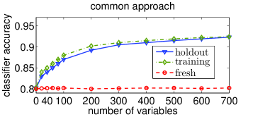
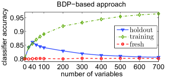
Figure 2. Reusing a holdout dataset in the common way can lead to overfitting.

Figure 3. Overfitting of reusing a holdout dataset is prevented in our Bayesian differential privacy-based approach.

5. Proofs

5.1. Useful Lemmas

Below we state several lemmas that will be used later to prove the theorems. Lemmas 2 and 3 below present the relationship between Bayesian differential privacy (BDP) and differential privacy (DP) when the tuple correlations can be arbitrary. Lemma 4 provides the corresponding result when the tuple correlations are modeled by a time-homogeneous Markov chain.

Lemma 2 ((Zhao et al., 2017)).

For a database with arbitrary tuple correlations, it holds that

$$\textrm{$\epsilon$-Bayesian differential privacy}\Longleftarrow\textrm{$\epsilon^{\prime}$-differential privacy}$$

(15) $$\textrm{for $\epsilon^{\prime}=\min_{i\in\{1,2,\ldots,n\}}\hskip 6.0pt\max_{\begin{subarray}{~{}}X_{Q_{i}}:~{}\text{\rm a {Markov quilt} of }X_{i}\\ X_{N_{i}}:~{}\text{\rm the {nearby set} associated with }X_{Q_{i}}\end{subarray}}\hskip 3.0pt\frac{\epsilon-4b_{i}}{|N_{i}|+1}$},$$

where $b_{i}\stackrel{{\scriptstyle\text{def}}}{{=}}\max\limits_{L\subseteq N_{i}}\mathcal{I}(X_{Q_{i}}\leftsquigarrow X_{i}\boldsymbol{\mid}X_{L})$, the meanings of a Markov quilt and its associated nearby set have been elaborated on Page 2.4, and $X_{Q_{i}}$ in (15) can iterate through the set of all Markov quilts of $X_{i}$, or just an arbitrary set containing some Markov quilts of $X_{i}$. Note that we can let $X_{Q_{i}}$ iterate through just an arbitrary set containing some Markov quilts of $X_{i}$, rather than iterating through the set of all Markov quilts of $X_{i}$, since (i) based on (15), letting $X_{Q_{i}}$ iterate a smaller set cannot make $\epsilon^{\prime}$ larger (i.e., it either induces a smaller $\epsilon^{\prime}$ or does not change $\epsilon^{\prime}$), and (ii) $\epsilon_{*}$-differential privacy with a smaller $\epsilon_{*}$ implies $\epsilon_{\#}$-differential privacy with a larger $\epsilon_{\#}$. In addition, as explained on Page 2.4, when we define a Markov quilt $X_{Q_{i}}$ for node $X_{i}$, the nearby set $X_{N_{i}}$ is also determined; i.e., $N_{i}$ is also determined. Given $N_{i}$, the set $L$ in the definition of $b_{i}$ iterates all subsets of $N_{i}$.

Lemma 3 ((Zhao et al., 2017)).

Letting $X_{Q_{i}}$ in (15) take just the Markov blanket of $X_{i}$ since the Markov blanket is a special case of the Markov quilt as discussed on Page 2.4, we can replace (15) by

$$\textrm{$\epsilon$-Bayesian differential privacy}\Longleftarrow\textrm{$\epsilon^{\prime}$-differential privacy}$$

$$\textrm{for $\epsilon^{\prime}=\min_{i\in\{1,2,\ldots,n\}}\hskip 6.0pt(\epsilon-4a_{i})$},$$

where $a_{i}\stackrel{{\scriptstyle\text{def}}}{{=}}\mathcal{I}(X_{M_{i}}\leftsquigarrow X_{i})=\ln\max\limits_{x_{i},x_{i}^{\prime},x_{M_{i}}}\frac{{\mathbb{P}}\left[{x_{M_{i}}\boldsymbol{\mid}x_{i}}\right]}{{\mathbb{P}}\left[{x_{M_{i}}\boldsymbol{\mid}x_{i}^{\prime}}\right]}$.

Lemma 4 ((Zhao et al., 2017)).

Consider a database with tuples modeled by a time-homogeneous Markov chain $X_{1}\rightarrow X_{2}\rightarrow\ldots\rightarrow X_{n}$ that is also aperiodic, irreducible and reversible. For this Markov chain, let $g$ be the spectral gap of the transition matrix; i.e., $g$ equals $1-\max\{|\lambda_{2}|,|\lambda_{3}|,\ldots,|\lambda_{n}|\}$ with the eigenvalues of the transition matrix in non-increasing order being $\lambda_{1}\geq\lambda_{2}\geq\ldots\geq\lambda_{n}$, where $\lambda_{1}=1$. Let $\rho$ be the probability of the least probable state in the stationary distribution of the Markov chain; i.e., $\rho$ equals $\min_{j\in S}d_{j}$ with vector $[d_{j}:j\in S]$ denoting the stationary distribution and $S$ denoting the state space. Let $c$ be an arbitrary constant satisfying $0<c<1/6$. With $d\stackrel{{\scriptstyle\text{def}}}{{=}}\Big{\lceil}\frac{1}{g}\ln\frac{e^{c\epsilon}+1}{\rho(e^{c\epsilon}-1)}\Big{\rceil}$, $t\stackrel{{\scriptstyle\text{def}}}{{=}}\big{\lfloor}\frac{1}{g}\ln\frac{1}{\rho}\big{\rfloor}$ and $\xi_{t+1}\stackrel{{\scriptstyle\text{def}}}{{=}}\frac{e^{-g(t+1)}}{\rho}$, then for $n\geq 2d$, $\epsilon$-Bayesian differential privacy is implied by $h(\epsilon,g,\rho)$-differential privacy, where

(16) $$h(\epsilon,g,\rho) \stackrel{{\scriptstyle\text{def}}}{{=}}\min\Bigg{\{}\frac{(1-6c)\epsilon}{2d-1},~{}\frac{(\frac{1}{3}-2c)\epsilon}{d+s}\Bigg{\}}.$$

5.2. Proof of Theorem 1 on Page 1

For an unknown distribution $\mathcal{D}$ over a discrete universe $\mathcal{X}$ of possible data points, a statistical query $Q$ asks for the expected value of some function $f:\mathcal{X}\rightarrow[0,1]$ on random draws from $\mathcal{D}$. On a database of $n$ records, the global sensitivity of a statistical query $Q$ is $\Delta_{Q}=1/n$. Substituting $\Delta_{Q}=1/n$ into Lemma 1 on Page 1, we obtain that under $\epsilon$-Bayesian differential privacy, if $\epsilon\leq{\tau}/3$, then ${\mathbb{P}}\left[{|Y(X)-Y(\mathcal{P})|\geq\tau}\right]\leq 4e^{-{\tau^{2}}n/9}$. Hence, to induce the desired ${\mathbb{P}}\left[{|Q_{i}(X)-Q_{i}(\mathcal{P})|\geq\tau}\right]\leq\beta$ in Theorem 1, we ensure $\epsilon\leq{\tau}/3$ and $4e^{-{\tau^{2}}n/9}\leq\beta$. From (Dwork et al., 2015a; Dwork and Roth, 2014), Algorithm 1 on Page 1 is $\epsilon_{*}$-differential private for $\epsilon_{*}=B\Delta_{Q}\cdot\big{(}\frac{1}{\sigma}+\frac{1}{\sigma_{2}}+\frac{2}{\sigma_{3}}\big{)}=\frac{9B\Delta_{Q}}{4\sigma}$. The above result and Lemma 2 together imply that Algorithm 1 is $\epsilon$-Bayesian differential private for $\epsilon=\min\limits_{i\in\{1,\ldots,n\}}~{}\max\limits_{\text{\rm Markov quilt }X_{Q_{i}}\text{ of }X_{i}}\frac{\frac{9B\Delta_{Q}}{4\sigma}-4b_{i}}{|N_{i}|+1}$. Then $\Delta_{Q}=1/n$ and the condition $\epsilon\leq{\tau}/3$ imply

(17) $$\textstyle{n\geq\max\limits_{i\in\{1,\ldots,n\}}~{}\min\limits_{\text{\rm Markov quilt }X_{Q_{i}}\text{ of }X_{i}}\frac{9B\cdot(|N_{i}|+1)}{4\sigma\cdot(\tau/3-4b_{i})}}.$$

In addition, the condition $4e^{-{\tau^{2}}n/9}\leq\beta$ implies

(18) $$\textstyle{n\geq\frac{9\ln(4/\beta)}{\tau^{2}}}.$$

Then with $n_{\#}(B,\sigma,\tau,\beta)$ defined as the maximum of the right hand sides of (17) and (18), we obtain that $n\geq n_{\#}(B,\sigma,\tau,\beta)$ suffices. We can also apply Lemma 3 instead of Lemma 2. In this case, (17) is replaced by

$$\textstyle{n\geq\max\limits_{i\in\{1,\ldots,n\}}\frac{9B}{4\sigma\cdot(\tau/3-4a_{i})}},$$

which together with (18) implies that $n\geq n_{*}(B,\sigma,\tau,\beta)$ suffices.  

5.3. Proof of Theorem 2 on Page 2

We prove Theorem 2 using the technique similar to that of (Dwork et al., 2015a, Theorem 25). For notation convenience in the analysis, we write “$\widehat{T}\leftarrow T+\textrm{Lap}(\sigma)$” in Lines 2 and 9 of Algorithm 1 as “$\widehat{T}\leftarrow T+\delta_{i}$”, where $\delta_{i}$ denotes $\textrm{Lap}(\sigma)$; i.e., $\delta_{i}$ is a fresh Laplace noise with parameter (i.e., scale) $\sigma$. Also, we write $Q_{i}(X)+\textrm{Lap}(\sigma_{2})$ in Line 10 of Algorithm 1 as $Q_{i}(X)+\xi_{i}$, where $\xi_{i}$ denotes $\textrm{Lap}(\sigma_{2})$; i.e., $\xi_{i}$ is a fresh Laplace noise with parameter $\sigma_{2}$. With the above changes, we restate Algorithm 1.

Algorithm 1 (Restated). A generalization-achieving algorithm (based on (Dwork et al., 2015a)) for adaptive queries $Q_{1},Q_{2},\ldots$, each with global sensitivity upper bounded by $\Delta_{Q}$.

0:  Holdout set $X$, training set $D$, noise rate $\sigma$, budget $B$, threshold $T$, queries $Q_{1},Q_{2},\ldots$

0:  A stream of answers

1:  let $\sigma_{2}\leftarrow 4\sigma$, and $\sigma_{3}\leftarrow 2\sigma$;

2:  let $\widehat{T}\leftarrow T+\delta_{i}$, where $\delta_{i}\leftarrow\textrm{Lap}(\sigma)$;     {Comment: $\textrm{Lap}(\sigma)$ means sampling a fresh Laplace noise with parameter (i.e., scale) $\sigma$.}

3:  for each query $Q_{i}$ do

4:     if $B<1$ then

5:        output “$\perp$”;

6:     else

7:        let $\gamma_{i}\leftarrow\textrm{Lap}(\sigma_{3})$;

8:        if $|Q_{i}(X)-Q_{i}(D)|+\gamma_{i}>\widehat{T}$ then

9:           let $B\leftarrow B-1$ and $\widehat{T}\leftarrow T+\delta_{i}$, where $\delta_{i}\leftarrow\textrm{Lap}(\sigma)$;

10:           output $Q_{i}(X)+\xi_{i}$, where $\xi_{i}\leftarrow\textrm{Lap}(\sigma_{2})$;

11:        else

12:           output $Q_{i}(D)$;

13:        end if

14:     end if

15:  end for

Recall that $a_{i}$ denotes the answer of Algorithm 1 on statistical query $Q_{i}$. In the result that we desire to prove, we bound the error between $a_{i}$ and $Q_{i}(\mathcal{P})$. This error can be decomposed as the difference between $a_{i}$ and $Q_{i}(X)$, and the difference between $Q_{i}(X)$ and $Q_{i}(\mathcal{P})$. More specifically, it holds that

$${\mathbb{P}}\left[{a_{i}\neq\perp\&|a_{i}-Q_{i}(\mathcal{P})|\geq\tau}\right]$$

(19) $$={\mathbb{P}}\left[{{a_{i}\neq\perp\&|a_{i}-Q_{i}(X)|\geq\frac{3+c}{4}\tau}}\right]+{\mathbb{P}}\left[{{|Q_{i}(\mathcal{P})-Q_{i}(X)|\geq\frac{1-c}{4}\tau}}\right].$$

A more formal reasoning that uses the union bound to establish (19) is presented below, where $\overline{A}$ means the complement of event $A$. We have

$${\mathbb{P}}\left[{a_{i}\neq\perp\&|a_{i}-Q_{i}(\mathcal{P})|\geq\tau}\right]$$

$$={\mathbb{P}}\left[{\overline{a_{i}=\perp~{}\text{or}~{}|a_{i}-Q_{i}(\mathcal{P})|<\tau}}\right]$$

$$\leq{\mathbb{P}}\left[{\overline{\bigg{(}a_{i}=\perp\text{or}\hskip 2.0pt|a_{i}-Q_{i}(X)|<\frac{3+c}{4}\tau\bigg{)}\&\bigg{(}|Q_{i}(\mathcal{P})-Q_{i}(X)|<\frac{1-c}{4}\tau\bigg{)}}}\right]$$

$$={\mathbb{P}}\left[{\overline{a_{i}=\perp\text{or}\hskip 2.0pt|a_{i}-Q_{i}(X)|<\frac{3+c}{4}\tau}~{}\text{or}~{}\overline{|Q_{i}(\mathcal{P})-Q_{i}(X)|<\frac{1-c}{4}\tau}}\right]$$

$$\leq{\mathbb{P}}\left[{\overline{a_{i}=\perp\text{or}\hskip 2.0pt|a_{i}-Q_{i}(X)|<\frac{3+c}{4}\tau}}\right]+{\mathbb{P}}\left[{\overline{|Q_{i}(\mathcal{P})-Q_{i}(X)|<\frac{1-c}{4}\tau}}\right]$$

(20) $$={\mathbb{P}}\left[{{a_{i}\neq\perp\&|a_{i}-Q_{i}(X)|\geq\frac{3+c}{4}\tau}}\right]+{\mathbb{P}}\left[{{|Q_{i}(\mathcal{P})-Q_{i}(X)|\geq\frac{1-c}{4}\tau}}\right].$$

To bound the second term in (20), we use Theorem 1 to obtain

(21) $$\text{for every }i:{\mathbb{P}}\left[{{|Q_{i}(\mathcal{P})-Q_{i}(X)|\geq\frac{1-c}{4}\tau}}\right]\leq\frac{\beta}{2m}$$

$$\text{ if }n\geq n_{\#}\bigg{(}B,\sigma,\frac{(1-c)\tau}{4},\frac{\beta}{2m}\bigg{)}.$$

where “for every $i$” means “$i\in\{1,\ldots,m\}$” (note that $m$ is the number of queries answered). Then (21) and the union bound together imply

(22) $${\mathbb{P}}\left[{\exists i:{|Q_{i}(\mathcal{P})-Q_{i}(X)|\geq\frac{1-c}{4}\tau}}\right]\leq\frac{\beta}{2}$$

$$\text{ if }n\geq n_{\#}\bigg{(}B,\sigma,\frac{(1-c)\tau}{4},\frac{\beta}{2m}\bigg{)},$$

where “$\exists i$” means “$\exists i\in\{1,\ldots,m\}$”.

Below we bound the first term in (20) by analyzing Algorithm 1. For the answer $a_{i}$ that is different from $\perp$, we bound the first term in (20) by considering two cases of Algorithm 1. First, if Line 10 of Algorithm 1 is executed, then $a_{i}=Q_{i}(X)+\xi_{i}$ and thus $|a_{i}-Q_{i}(X)|=|\xi_{i}|$. Second, if Line 12 of Algorithm 1 is executed, then $|Q_{i}(X)-Q_{i}(D)|+\gamma_{i}\leq\widehat{T}$ and $a_{i}=Q_{i}(D)$, yielding $|a_{i}-Q_{i}(X)|=|Q_{i}(D)-Q_{i}(X)|\leq\widehat{T}-\gamma_{i}=T+\delta_{i}-\gamma_{i}$ and furthermore $|a_{i}-Q_{i}(X)|\leq T+|\delta_{i}|+|\gamma_{i}|$. Summarizing the two cases above, we obtain

$${\mathbb{P}}\left[{\exists i:{a_{i}\neq\perp~{}\&~{}|a_{i}-Q_{i}(X)|\geq\frac{3+c}{4}\cdot\tau}}\right]$$

$$\leq\max\bigg{\{}{\mathbb{P}}\left[{\exists i:|\xi_{i}|\geq\frac{3+c}{4}\tau}\right],{\mathbb{P}}\left[{\exists i:|\delta_{i}|+|\gamma_{i}|\geq\frac{3+c}{4}\tau-T}\right]\bigg{\}}$$

(23) $$\leq\max\bigg{\{}{\mathbb{P}}\left[{\exists i:|\xi_{i}|\geq\frac{3+c}{4}\tau}\right],{\mathbb{P}}\left[{\exists i:|\delta_{i}|+|\gamma_{i}|\geq\frac{1-c}{4}\tau}\right]\bigg{\}},$$

where the last step uses $T=\frac{(1+c)\tau}{2}$.

Since $\xi_{i}$ obeys a Laplace distribution with parameter $4\sigma$, where $\sigma\stackrel{{\scriptstyle\text{def}}}{{=}}\frac{(1-c)\tau}{12\ln(4m/\beta)}$ from the condition, it holds that

(24) $$\text{for every }i:{\mathbb{P}}\left[{|\xi_{i}|\geq\frac{3+c}{4}\tau}\right]=\exp\bigg{\{}-\frac{\frac{3+c}{4}\cdot\tau}{4\sigma}\bigg{\}}\leq\frac{\beta}{4m},$$

where the last step uses $\frac{3+c}{16}\geq\frac{1-c}{12}$. Then (24) and the union bound yield

(25) $${\mathbb{P}}\left[{\exists i:|\xi_{i}|\geq\frac{3+c}{4}\tau}\right]\leq\frac{\beta}{4}.$$

To bound ${\mathbb{P}}\left[{\exists i:|\delta_{i}|+|\gamma_{i}|\geq\frac{1-c}{4}\tau}\right]$, we use the union bound to derive

$${\mathbb{P}}\left[{\exists i:|\delta_{i}|+|\gamma_{i}|\geq\frac{1-c}{4}\tau}\right]$$

$$={\mathbb{P}}\left[{\overline{\forall i:|\delta_{i}|+|\gamma_{i}|<\frac{1-c}{4}\tau}}\right]$$

$$\leq{\mathbb{P}}\left[{\overline{\bigg{(}\forall i:|\delta_{i}|<\frac{1-c}{12}\tau\bigg{)}~{}\&~{}\bigg{(}\forall i:|\gamma_{i}|<\frac{1-c}{6}\tau\bigg{)}}}\right]$$

$$={\mathbb{P}}\left[{\overline{\bigg{(}\forall i:|\delta_{i}|<\frac{1-c}{12}\tau\bigg{)}}\text{ or }\overline{\bigg{(}\forall i:|\gamma_{i}|<\frac{1-c}{6}\tau\bigg{)}}}\right]$$

$$\leq{\mathbb{P}}\left[{\overline{\bigg{(}\forall i:|\delta_{i}|<\frac{1-c}{12}\tau\bigg{)}}}\right]+{\mathbb{P}}\left[{\overline{\bigg{(}\forall i:|\gamma_{i}|<\frac{1-c}{6}\tau\bigg{)}}}\right]$$

(26) $$={\mathbb{P}}\left[{\exists i:|\delta_{i}|\geq\frac{1-c}{12}\tau}\right]+{\mathbb{P}}\left[{\exists i:|\gamma_{i}|\geq\frac{1-c}{6}\tau}\right].$$

Since $\delta_{i}$ obeys a Laplace distribution with parameter $\sigma$, and $\gamma_{i}$ obeys a Laplace distribution with parameter $2\sigma$, then given $\sigma=\frac{(1-c)\tau}{12\ln(4m/\beta)}$, we obtain

(27) $$\text{for every }i:{\mathbb{P}}\left[{|\delta_{i}|\geq\frac{1-c}{12}\cdot\tau}\right]=\exp\bigg{\{}-\frac{\frac{1-c}{12}\cdot\tau}{\sigma}\bigg{\}}=\frac{\beta}{4m}$$

and

(28) $$\text{for every }i:{\mathbb{P}}\left[{|\gamma_{i}|\geq\frac{1-c}{6}\cdot\tau}\right]=\exp\bigg{\{}-\frac{\frac{1-c}{6}\cdot\tau}{2\sigma}\bigg{\}}=\frac{\beta}{4m}.$$

Then using the union bound together with (27) and (28), we have

(29) $${\mathbb{P}}\left[{\exists i:|\delta_{i}|\geq\frac{1-c}{12}\cdot\tau}\right]=\exp\bigg{\{}-\frac{\frac{1-c}{12}\cdot\tau}{\sigma}\bigg{\}}=\frac{\beta}{4}$$

and

(30) $${\mathbb{P}}\left[{\exists i:|\gamma_{i}|\geq\frac{1-c}{6}\cdot\tau}\right]=\exp\bigg{\{}-\frac{\frac{1-c}{6}\cdot\tau}{2\sigma}\bigg{\}}=\frac{\beta}{4}.$$

Applying (29) and (30) to (26), we derive

(31) $${\mathbb{P}}\left[{\exists i:|\delta_{i}|+|\gamma_{i}|\geq\frac{1-c}{4}\tau}\right] \leq\frac{\beta}{2}.$$

Substituting (25) and (31) into (23), we obtain

(32) $${\mathbb{P}}\left[{\exists i:{a_{i}\neq\perp~{}\&~{}|a_{i}-Q_{i}(X)|\geq\frac{3+c}{4}\cdot\tau}}\right]\leq\frac{\beta}{2}.$$

Using (22) and (32) in (20), we have

(33) $${\mathbb{P}}\left[{\exists i:a_{i}\neq\perp~{}\&~{}|a_{i}-Q_{i}(\mathcal{P})|\geq\tau}\right]\leq\beta.$$

$$\text{ if }n\geq n_{\#}\bigg{(}B,\sigma,\frac{(1-c)\tau}{4},\frac{\beta}{2m}\bigg{)}.$$

To complete the proof, we will show that $Z_{i}<B$ is a subevent of $a_{i}\neq\perp$ (i.e., if $Z_{i}<B$ then $a_{i}\neq\perp$) so that

$${\mathbb{P}}\left[{\exists i:Z_{i}<B~{}\&~{}|a_{i}-Q_{i}(\mathcal{P})|\geq\tau}\right]$$

$$\leq{\mathbb{P}}\left[{\exists i:a_{i}\neq\perp~{}\&~{}|a_{i}-Q_{i}(\mathcal{P})|\geq\tau}\right],$$

where $Z_{i}\stackrel{{\scriptstyle\text{def}}}{{=}}\big{|}\{j\leq i:|Q_{j}(D)-Q_{j}(\mathcal{P})|\geq c\tau\}\big{|}$ denotes the counter of overfitting. For every $j\leq i$ that reduces the budget $B$ in Algorithm 1 (i.e., Line 9 of Algorithm 1 is executed), it follows that

$$|Q_{j}(D)-Q_{j}(\mathcal{P})| \geq|Q_{j}(X)-Q_{j}(D)|-|Q_{j}(\mathcal{P})-Q_{j}(X)|$$

$$\geq|\widehat{T}-\gamma_{j}|-|Q_{j}(\mathcal{P})-Q_{j}(X)|$$

$$\geq|T+\delta_{j}-\gamma_{j}|-|Q_{j}(\mathcal{P})-Q_{j}(X)|$$

(34) $$\geq T-|\delta_{j}|-|\gamma_{j}|-|Q_{j}(\mathcal{P})-Q_{j}(X)|.$$

Then applying $T=\frac{1+c}{2}\tau$, $|\delta_{j}|<\frac{1-c}{12}\tau$, $|\gamma_{j}|<\frac{1-c}{6}\tau$ and $|Q_{j}(\mathcal{P})-Q_{j}(X)|<\frac{1-c}{4}\tau$ to (34), we find

$$|Q_{j}(D)-Q_{j}(\mathcal{P})| \geq\frac{1+c}{2}\tau-\frac{1-c}{12}\tau-\frac{1-c}{6}\tau-\frac{1-c}{4}\tau=c\tau.$$

Hence, if $Z_{i}<B$, then the budget $B$ in Algorithm 1 is still at least $1$, and hence $a_{i}\neq\perp$. This along with (33) implies that

$${\mathbb{P}}\left[{\exists i:a_{i}\neq\perp~{}\&~{}|a_{i}-Q_{i}(\mathcal{P})|\geq\tau}\right]\leq\beta.$$

(35) $$\text{ if }n\geq n_{\#}\bigg{(}B,\sigma,\frac{(1-c)\tau}{4},\frac{\beta}{2m}\bigg{)}.$$

Given the condition $\sigma=\frac{(1-c)\tau}{12\ln(4m/\beta)}$ and $n_{\#}(\cdot)$ defined in Theorem 1, we obtain from (35) that

$$n \geq n_{\#}\bigg{(}B,\frac{(1-c)\tau}{12\ln(4m/\beta)},\frac{(1-c)\tau}{4},\frac{\beta}{2m}\bigg{)}$$

(38) $$=\max\left\{\begin{array}[]{l}\frac{9\ln(4/\beta)}{\tau^{2}},\\ \max\limits_{i\in\{1,\ldots,n\}}~{}\min\limits_{\text{\rm Markov quilt }X_{Q_{i}}\text{ of }X_{i}}~{}\frac{9B\cdot(|N_{i}|+1)}{4\cdot\frac{(1-c)\tau}{12\ln(4m/\beta)}\cdot(\tau/3-4b_{i})}\end{array}\right\}$$

(40) $$=\textstyle{O\Bigg{(}\begin{array}[]{l}B\ln\frac{m}{\beta}\cdot\max\limits_{i\in\{1,\ldots,n\}}~{}\min\limits_{\text{\rm Markov quilt }X_{Q_{i}}\text{ of }X_{i}}~{}\frac{|N_{i}|+1}{\tau\cdot(\tau/3-4b_{i})}\end{array}\Bigg{)}}.$$

Hence, we have proved the result for arbitrary correlations between data samples in Theorem 2. Now we establish the result of in Theorem 2 when the Markov chain represents the correlations between data samples: on a time-homogeneous Markov chain that is also aperiodic, irreducible and reversible, the condition on $n$ in (40) becomes $n=O\big{(}\frac{B\ln(1/\tau)}{\tau^{2}}\cdot\ln\frac{m}{\beta}\big{)}$. To this end, given (40), then with $\epsilon$ being $\tau/3$, we will evaluate

(41) $$\textstyle{\max\limits_{i\in\{1,\ldots,n\}}~{}\min\limits_{\text{\rm Markov quilt }X_{Q_{i}}\text{ of }X_{i}}\frac{|N_{i}|+1}{\epsilon-4b_{i}}}.$$

As shown in Lemma 2 on Page 2 above, $\epsilon$-Bayesian differential privacy is implied by $\epsilon^{\prime}$-differential privacy, for
$\epsilon^{\prime}\stackrel{{\scriptstyle\text{def}}}{{=}}\min\limits_{i\in\{1,\ldots,n\}}~{}\max\limits_{\text{\rm Markov quilt }X_{Q_{i}}\text{ of }X_{i}}\frac{\epsilon-4b_{i}}{|N_{i}|+1}$. Then the term in (41) equals ${1}/{\epsilon^{\prime}}$. The above result holds because for any sequence $s_{i}$, we can write $\frac{1}{\max s_{i}}$ as $\min\frac{1}{s_{i}}$, and write $\frac{1}{\min s_{i}}$ as $\max\frac{1}{s_{i}}$. On a time-homogeneous Markov chain $X_{1}\rightarrow X_{2}\rightarrow\ldots\rightarrow X_{n}$ that is also aperiodic, irreducible and reversible, the quantity $\rho>0$ is the probability of the least probable state in the stationary distribution of the Markov chain; i.e., $\rho$ equals $\min_{j\in S}d_{j}$ with vector $[d_{j}:j\in S]$ denoting the stationary distribution and $S$ denoting the state space. The term $g$ is the spectral gap of the transition matrix; i.e., $g$ equals $1-\max\{|\lambda_{2}|,|\lambda_{3}|,\ldots,|\lambda_{n}|\}$ with the eigenvalues of the transition matrix in non-increasing order being $\lambda_{1}\geq\lambda_{2}\geq\ldots\geq\lambda_{n}$, where $\lambda_{1}=1$. Then Lemma 4 on Page 4 above shows that ${\epsilon^{\prime}}$ above can be replaced by $h(\epsilon,g,\rho)$ as follows:

(42) $$h(\epsilon,g,\rho) \stackrel{{\scriptstyle\text{def}}}{{=}}\min\Bigg{\{}\frac{(1-6c)\epsilon}{2d-1},\frac{(\frac{1}{3}-2c)\epsilon}{d+s}\Bigg{\}},$$

where $d\stackrel{{\scriptstyle\text{def}}}{{=}}\Big{\lceil}\frac{1}{g}\ln\frac{e^{c\epsilon}+1}{\rho(e^{c\epsilon}-1)}\Big{\rceil}$ and $s\stackrel{{\scriptstyle\text{def}}}{{=}}\Big{\lfloor}\frac{1}{g}\ln\frac{e^{\epsilon/6}+1}{\rho(e^{\epsilon/6}-1)}\Big{\rfloor}$. We further prove that $1/[h(\epsilon,g,\rho)]=O\big{(}\frac{1}{\tau}\ln\frac{1}{\tau}\big{)}$ follows. Clearly, we obtain

(43) $$d\leq\frac{1}{g}\ln\frac{e^{c\epsilon}+1}{\rho(e^{c\epsilon}-1)}+1=\frac{1}{g}\ln\bigg{(}1+\frac{2}{e^{c\epsilon}-1}\bigg{)}+\frac{1}{g}\ln\frac{1}{\rho}+1$$

and

(44) $$s\leq\frac{1}{g}\ln\frac{e^{\epsilon/6}+1}{\rho(e^{\epsilon/6}-1)}=\frac{1}{g}\ln\bigg{(}1+\frac{2}{e^{\epsilon/6}-1}\bigg{)}+\frac{1}{g}\ln\frac{1}{\rho}.$$

Given $\epsilon=\tau/3$, $0<\tau\leq 1$, $0<c<1/6$, we have $c\epsilon<\epsilon/6\leq\tau/18\leq 1/18$, implying $e^{c\epsilon}<e^{\epsilon/6}\leq e^{1/18}$. Then it holds that $\frac{2}{e^{c\epsilon}-1}>\frac{2}{e^{\epsilon/6}-1}\geq\frac{2}{e^{1/18}-1}>1$. Since $\ln(1+a)\leq\ln(2a)$ holds for $a\geq 1$, we further obtain $\ln(1+\frac{2}{e^{c\epsilon}-1})\leq\ln\frac{4}{e^{c\epsilon}-1}\leq\ln\frac{4}{c\epsilon}=\ln\frac{12}{c\tau}$ and $\ln(1+\frac{2}{e^{\epsilon/6}-1})\leq\ln\frac{4}{e^{\epsilon/6}-1}\leq\ln\frac{4}{\epsilon/6}=\ln\frac{24}{\epsilon}=\ln\frac{72}{\tau}$. The application of these to (43) and (44) yields

(45) $$d\leq\frac{1}{g}\ln\frac{12}{c\tau}+\frac{1}{g}\ln\frac{1}{\rho}+1$$

and

(46) $$s\leq\frac{1}{g}\ln\frac{72}{\tau}+\frac{1}{g}\ln\frac{1}{\rho}.$$

Using (45) and (46) in (42), we get

$$h(\epsilon,g,\rho) \stackrel{{\scriptstyle\text{def}}}{{=}}\min\Bigg{\{}\frac{(1-6c)\epsilon}{2d-1},\frac{(\frac{1}{3}-2c)\epsilon}{d+s}\Bigg{\}}$$

$$\geq\min\Bigg{\{}\frac{(1-6c)\cdot\tau/3}{\frac{2}{g}\ln\frac{12}{c\rho}+\frac{2}{g}\ln\frac{1}{\tau}+1},$$

$$\hskip 30.0pt\frac{(\frac{1}{3}-2c)\cdot\tau/3}{\frac{1}{g}\ln\frac{12}{c\rho}+\frac{1}{g}\ln\frac{1}{\tau}+1+\frac{1}{g}\ln\frac{72}{\rho}+\frac{1}{g}\ln\frac{1}{\tau}}\Bigg{\}},$$

which further implies

$$\frac{1}{h(\epsilon,g,\rho)} \leq\min\Bigg{\{}\frac{\frac{2}{g}\ln\frac{12}{c\rho}+\frac{2}{g}\ln\frac{1}{\tau}+1}{(1-6c)\cdot\tau/3},$$

(47) $$\hskip 10.0pt\frac{\frac{1}{g}\ln\frac{12}{c\rho}+\frac{1}{g}\ln\frac{1}{\tau}+1+\frac{1}{g}\ln\frac{72}{\rho}+\frac{1}{g}\ln\frac{1}{\tau}}{(\frac{1}{3}-2c)\cdot\tau/3}\Bigg{\}}.$$

Ignoring the constants in (47), we have

(48) $$\frac{1}{h(\epsilon,g,\rho)} =O\bigg{(}\frac{1}{\tau}\ln\frac{1}{\tau}\bigg{)}.$$

As noted, $h(\epsilon,g,\rho)$ is a lower bound of ${\epsilon^{\prime}}$, which implies that $1/[h(\epsilon,g,\rho)]$ is an upper bound of ${1}/{\epsilon^{\prime}}$ (i.e., the term in (41)). Then from (48), the term in (41) can be expressed as $O\big{(}\frac{1}{\tau}\ln\frac{1}{\tau}\big{)}$. From $\epsilon=\tau/3$, this means that $n$ specified in (40) becomes $n=O\big{(}\frac{B\ln(1/\tau)}{\tau^{2}}\cdot\ln\frac{m}{\beta}\big{)}$. Hence, the proof of Theorem 2 is now completed.  

6. Related Work

In many practical applications, statistical learning is often adaptive—the queries on a dataset depend on previous interactions with the same dataset. However, generalization guarantees are traditionally given in a non-adaptive model. Recent studies by Hardt and Ullman (Hardt and Ullman, 2014) as well as Dwork et al. (Dwork et al., 2015a, b, c) provide generalization bounds in adaptive statistical learning, while Dwork et al. (Dwork et al., 2015a, b, c) also propose mechanisms via differential privacy and max-information. Differential privacy means that an adversary given access to the output does not have much confidence to determine whether the output was sampled from the probability distribution generated by the algorithm under a database $x$ or under a neighboring database $x^{\prime}$ that differs from $x$ in one record. Specifically, a randomized algorithm $Y$ satisfies $\epsilon$-differential privacy if for all neighboring databases $x$, $x^{\prime}$ and any subset $\mathcal{Y}$ of the ouput range of the mechanism $Y$, it holds that ${\mathbb{P}}\left[{Y(x)\in\mathcal{Y}}\right]\leq e^{\epsilon}{\mathbb{P}}\left[{Y(x^{\prime})\in\mathcal{Y}}\right].$ The notion of max-information gives generalization since it upper bounds the probability of “bad events” that can occur as a result of the dependence of the output variable $Y(X)$ on the input variable $X$.

Rogers et al. (Rogers et al., 2016) show the connection between approximate differential privacy and max-information, and prove that the connection holds only for data drawn from product distributions, where approximate differential privacy (ADP) (Dwork et al., 2006a) relaxes differential privacy so that $(\epsilon,\delta)$-ADP means the probabilities that the same output is seen on neighboring databases $x$ and $x^{\prime}$ (differing in one record) is bounded by a factor $e^{\epsilon}$, in addition to a small additive probability $\delta$; i.e., ${\mathbb{P}}\left[{Y(x)\in\mathcal{Y}}\right]\leq e^{\epsilon}{\mathbb{P}}\left[{Y(x^{\prime})\in\mathcal{Y}}\right]+\delta$ for any subset $\mathcal{Y}$ of the ouput range of the mechanism $Y$. Very recently, Bassily and Freund (Bassily and Freund, 2016) propose an algorithmic stability notion called typical stability which provides generalization for a broader class of queries than that of bounded-sensitivity queries (bounded sensitivity is often required by differential privacy). Typical stability means that the output of a query is “well-concentrated” around its expectation with respect to the underlying distribution on the dataset. Cummings et al. (Cummings et al., 2016) introduce different generalization notions and discuss their relationships with differential privacy. Russo and Zou (Russo and Zou, 2016) present a mutual-information framework for adaptive statistical learning and compare it with max-information. Blum and Hardt (Blum and Hardt, 2015) design an algorithm to maintain an accurate leaderboard for machine learning competitions (such as those organized by Kaggle Inc. at http://www.kaggle.com/ ), where submissions can be adaptive.

Since differential privacy was proposed to quantify privacy analysis (Dwork, 2006; Dwork et al., 2006b), this notion has received much attention in the literature (Blocki et al., 2016; Tramèr et al., 2015; Qin et al., 2016; Jiang et al., 2013; Song and Chaudhuri, 2017). Kifer and Machanavajjhala (Kifer and Machanavajjhala, 2011) observe that differential privacy may not work well when the data tuples are correlated in between. To generalize differential privacy, Kifer and Machanavajjhala (Kifer and Machanavajjhala, 2012) introduce the Pufferfish framework by considering the generation of the database and the adversarial belief about the database. A subclass of the Pufferfish framework, called the Blowfish framework, is investigated by He et al. (He et al., 2014). Blowfish privacy imposes deterministic policy constraints rather than probabilistic correlations to model adversarial knowledge. A general mechanism to achieve Pufferfish privacy is recently proposed by Song et al. (Song et al., 2017). Xiao and Xiong (Xiao and Xiong, 2015) incorporate temporal correlations into differential privacy in the context of location privacy. Chen et al. (Chen et al., 2014) and Zhu et al. (Zhu et al., 2015) give different algorithms for privacy under data correlations. To improve the utilities of these algorithms, Liu et al. (Liu et al., 2016) present a Laplace mechanism that handles pairwise correlations. Yang et al. (Yang et al., 2015) consider different adversary models and formalize the notion of Bayesian differential privacy that tackles tuple correlations as well. Yang et al. (Yang et al., 2015) further introduce a mechanism that is only for the sum query on a Gaussian Markov random field with positive correlations and its extension to a discrete domain. For Bayesian differential privacy, Zhao et al. (Zhao et al., 2017) present mechanisms for databases with arbitrary tuple correlations and elaborate the case of tuple correlations being modeled by a Markov chain.

7. Conclusion

Recently, Dwork et al. (Dwork et al., 2015a, b, c) show that the holdout dataset from i.i.d. data samples can be reused in adaptive statistical learning, if the estimates are perturbed and coordinated using techniques developed for differential privacy, which is a widely used notion to define privacy. Yet, the results of Dwork et al. (Dwork et al., 2015a, b, c) are applicable to only the case of i.i.d. samples. In this paper, we show that Bayesian differential privacy can be used to ensure statistical validity in adaptive statistical learning, where Bayesian differential privacy is introduced by Yang et al. (Yang et al., 2015) to extend differential privacy for addressing the case when data records are correlated. Specifically, we prove that the holdout dataset from correlated samples can be reused in adaptive statistical learning, if the estimates are perturbed and coordinated using techniques satisfying Bayesian differential privacy. Our results generalize those of Dwork et al. (Dwork et al., 2015a, b, c) for i.i.d. samples to arbitrarily correlated data.

 

Appendix

A.1. Establishing Theorem 3

To begin with, we first define martingale and Doob martingale that will be used in the proof of Theorem 3. A sequence of random variables $Z_{0},Z_{1},\ldots$ is referred to as a martingale (Colantonio et al., 2009) if $\mathbb{E}[Z_{i+1}|Z_{0},\ldots,Z_{i}]=Z_{i}$ and $\mathbb{E}[|Z_{i}|]<\infty$ for $i=0,1,\ldots$, where $\mathbb{E}[\cdot]$ stands for the expected value of a random variable. A Doob martingale (Colantonio et al., 2009) is a martingale constructed using the following general approach. Let $X_{0},X_{1},\ldots,X_{m}$ be a sequence of random variables, and let $Y$ be a random variable with $\mathbb{E}[|Y|]<\infty$ (In general, $Y$ is a function of $X_{0},X_{1},\ldots,X_{m}$). Then the sequence consisting of $Z_{i}=\mathbb{E}[Y|X_{0},\ldots,X_{i}]$ for $i=0,1,\ldots,m$ gives a Doob martingale. Note that in the expression $Z_{i}=\mathbb{E}[Y|X_{0},\ldots,X_{i}]$, the expectation is only taken over $X_{i+1},X_{i+2},\ldots,X_{m}$ while $X_{0},\ldots,X_{i}$ are kept as random variables, so $Z_{i}$ is still a random variable.

The Azuma-Hoeffding inequality (see Lemma 2 of (Bollobás et al., 2001)) presented below is widely used in the analysis of martingales.

Lemma 5 (Azuma-Hoeffding Inequality as Lemma 2 of (Bollobás et al., 2001)).

If $Z_{i}|_{i=0,\ldots,n}$ is a martingale such that $|Z_{i}-Z_{i-1}|\leq c$ for each $i=1,\ldots,n$, then ${\mathbb{P}}\left[{Z_{n}-Z_{0}\geq t}\right]\leq\exp\big{(}\frac{-t^{2}}{2nc^{2}}\big{)}$.

We now continue the proof ofTheorem 3. We first fix $y\in\mathcal{Y}$, and define a function $g(x)\stackrel{{\scriptstyle\text{def}}}{{=}}\ln\left(\frac{\mathbb{P}[Y=y\boldsymbol{\mid}X=x]}{\mathbb{P}[Y=y]}\right)$. For function $g$, we will define a Doob martingale $Z_{i}|_{i=0,\ldots,n}$ with respect to $X_{i}|_{i=1,\ldots,n}$. Specifically, we define

$$Z_{i}(x_{1},\ldots,x_{i})\stackrel{{\scriptstyle\text{def}}}{{=}}\mathbb{E}_{X_{i+1},\ldots,X_{n}}[g(x_{1},\ldots,x_{i},X_{i+1},\ldots,X_{n})]$$

for $i=0,\ldots,n$; i.e., given $x_{1},\ldots,x_{i}$, we take the expectation of
$g(x_{1},\ldots,x_{i},X_{i+1},\ldots,X_{n})$ with respect to $X_{i+1},\ldots,X_{n}$, and obtain
$Z_{i}(x_{1},\ldots,x_{i})$. For simplicity, we write the sequence $X_{i+1},\ldots,X_{n}$ as $X_{i+1:n}$, and write the sequence $x_{1},\ldots,x_{i}$ as $x_{1:i}$, and so on. Then

(49) $$Z_{i}(x_{1:i}) =\mathbb{E}_{X_{i+1:n}}[g(x_{1:i},X_{i+1:n})]$$

(50) $$=\sum_{x_{i+1:n}}g(x_{1:i},x_{i+1:n}){\mathbb{P}}\left[{x_{i+1:n}\boldsymbol{\mid}x_{1:i}}\right].$$

Replacing $i$ with $i-1$ in (50), we obtain

$$Z_{i-1}(x_{1:i-1})$$

$$=\mathbb{E}_{X_{i:n}}[g(x_{1:{i-1}},X_{i:n})]$$

(51) $$=\sum_{x_{i}^{\prime}}\sum_{x_{i+1:n}}g(x_{1:i-1},x_{i}^{\prime},x_{i+1:n}){\mathbb{P}}\left[{x_{i}^{\prime},x_{i+1:n}\boldsymbol{\mid}x_{1:i-1}}\right].$$

To find the connection between (50) and (51), we first note
${\mathbb{P}}\left[{x_{i}^{\prime},x_{i+1:n}\boldsymbol{\mid}x_{1:i-1}}\right]={\mathbb{P}}\left[{x_{i+1:n}\boldsymbol{\mid}x_{1:i-1},x_{i}^{\prime}}\right]\cdot{\mathbb{P}}\left[{x_{i}^{\prime}\boldsymbol{\mid}x_{1:i-1}}\right]$ by the chain rule; put it in detail, we have

$${\mathbb{P}}\left[{x_{i}^{\prime},x_{i+1:n}\boldsymbol{\mid}x_{1:i-1}}\right]$$

$$=\frac{{\mathbb{P}}\left[{x_{1:i-1},x_{i}^{\prime},x_{i+1:n}}\right]}{{\mathbb{P}}\left[{x_{1:i-1}}\right]}$$

$$=\frac{{\mathbb{P}}\left[{x_{1:i-1},x_{i}^{\prime},x_{i+1:n}}\right]}{{\mathbb{P}}\left[{x_{1:i-1},x_{i}^{\prime}}\right]}\cdot\frac{{\mathbb{P}}\left[{x_{1:i-1},x_{i}^{\prime}}\right]}{{\mathbb{P}}\left[{x_{1:i-1}}\right]}$$

(52) $$={\mathbb{P}}\left[{x_{i+1:n}\boldsymbol{\mid}x_{1:i-1},x_{i}^{\prime}}\right]\cdot{\mathbb{P}}\left[{x_{i}^{\prime}\boldsymbol{\mid}x_{1:i-1}}\right].$$

Substituting (52) into (51), we establish

$$Z_{i-1}(x_{1:i-1})$$

$$=\mathbb{E}_{X_{i:n}}[g(x_{1:{i-1}},X_{i:n})]$$

(55) $$=\sum_{x_{i}^{\prime}}\sum_{x_{i+1:n}}\begin{array}[]{l}g(x_{1:i-1},x_{i}^{\prime},x_{i+1:n}){\mathbb{P}}\left[{x_{i+1:n}\boldsymbol{\mid}x_{1:i-1},x_{i}^{\prime}}\right]\\ \cdot{\mathbb{P}}\left[{x_{i}^{\prime}\boldsymbol{\mid}x_{1:i-1}}\right]\end{array}$$

(56) $$=\sum_{x_{i}^{\prime}}\big{\{}\mathbb{E}_{X_{i+1:n}}[g(x_{1:i-1},x_{i}^{\prime},X_{i+1:n})]\cdot{\mathbb{P}}\left[{x_{i}^{\prime}\boldsymbol{\mid}x_{1:i-1}}\right]\big{\}}.$$

In view of (49) and (56), we will prove $|Z_{i}-Z_{i-1}|\leq\epsilon$ by showing for any $x_{i}^{\prime}$ that

(57) $$|\mathbb{E}_{X_{i+1:n}}[g(x_{1:i-1},x_{i}^{\prime},X_{i+1:n})]-\mathbb{E}_{X_{i+1:n}}[g(x_{1:i},X_{i+1:n})]|\leq\epsilon.$$

We have

(58) $$\mathbb{E}_{X_{i+1:n}}[g(x_{1:i-1},x_{i}^{\prime},X_{i+1:n})]=\ln\frac{\mathbb{P}[Y(x_{1:i-1},x_{i}^{\prime},X_{i+1:n})=y]}{\mathbb{P}[Y=y]}$$

and

(59) $$\mathbb{E}_{X_{i+1:n}}[g(x_{1:i},X_{i+1:n})]=\ln\frac{\mathbb{P}[Y(x_{1:i},X_{i+1:n})=y]}{\mathbb{P}[Y=y]}.$$

Under $\epsilon$-Bayesian differential privacy, it holds by definition that $e^{-\epsilon}\leq\frac{\mathbb{P}[Y(x_{1:i-1},x_{i},X_{i+1:n})=y]}{\mathbb{P}[Y(x_{1:i-1},x_{i}^{\prime},X_{i+1:n})=y]}\leq e^{\epsilon}$, which with (58) and (59) implies (57). Since (57) holds for any $x_{i}^{\prime}$, we then obtain $|Z_{i}-Z_{i-1}|\leq\epsilon$ from (49) and (56). Since $i$ can iterate through $\{1,\ldots,n\}$, we have proved $|Z_{i}-Z_{i-1}|\leq\epsilon$ for $i=1,\ldots,n$. Then we use the Azuma-Hoeffding inequality (i.e., Lemma 5 above) and obtain ${\mathbb{P}}\left[{Z_{n}-Z_{0}\geq t}\right]\leq\exp\big{(}\frac{-t^{2}}{2n{\epsilon}^{2}}\big{)}$ for any $t>0$. By definition, $Z_{n}(x_{1:n})=g(x_{1:n})=g(x)$ and $Z_{0}=\mathbb{E}_{X_{1:n}}[g(X_{1:n})]=\mathbb{E}_{X}[g(X)]$. Hence, it follows that

(60) $${\mathbb{P}}\left[{g(x)-\mathbb{E}_{X}[g(X)]\geq t}\right] \leq\exp\bigg{(}\frac{-t^{2}}{2n{\epsilon}^{2}}\bigg{)}.$$

We now evaluate $\mathbb{E}_{X}[g(X)]$ as follows.

$$\mathbb{E}_{X}[g(X)] =\mathbb{E}_{X}\bigg{[}\ln\frac{{\mathbb{P}}\left[{Y(X)=y}\right]}{Y=y}\bigg{]}$$

$$=\mathbb{E}_{X}[\ln{\mathbb{P}}\left[{Y(X)=y}\right]]-\mathbb{E}_{X}[\ln{\mathbb{P}}\left[{Y=y}\right]]$$

(61) $$=\mathbb{E}_{X}[\ln{\mathbb{P}}\left[{Y(X)=y}\right]]-\ln{\mathbb{P}}\left[{Y=y}\right].$$

Since the natural logarithm $\ln$ is a convex function, we use Jensen’s inequality to obtain

(62) $$\mathbb{E}_{X}[\ln{\mathbb{P}}\left[{Y(X)=y}\right]]\leq\ln[\mathbb{E}_{X}{\mathbb{P}}\left[{Y(X)=y}\right]]=\ln{\mathbb{P}}\left[{Y=y}\right].$$

Using (62) in (61), we have $\mathbb{E}_{X}[g(X)]\leq 0$, which along with (60) further yields

(63) $${\mathbb{P}}\left[{g(x)\geq t}\right] \leq\exp\bigg{(}\frac{-t^{2}}{2n{\epsilon}^{2}}\bigg{)}.$$

For an integer $i\geq 1$, we define $t_{i}\stackrel{{\scriptstyle\text{def}}}{{=}}2{\epsilon}^{2}n+\epsilon\sqrt{2n\ln(2^{i}/\beta)}$ and define $B_{i}\stackrel{{\scriptstyle\text{def}}}{{=}}\big{\{}x\boldsymbol{\mid}t_{i}<g(x)\leq t_{i+1}\big{\}}$. Let $B_{y}\stackrel{{\scriptstyle\text{def}}}{{=}}\big{\{}x\boldsymbol{\mid}g(x)>t_{1}\big{\}}=\bigcup_{i\geq 1}B_{i}$. By Bayes’ rule, for every $x\in B_{i}$, it holds that

(64) $$\frac{\mathbb{P}[X=x\boldsymbol{\mid}Y=y]}{\mathbb{P}[X=x]} =\frac{\mathbb{P}[Y=y\boldsymbol{\mid}X=x]}{\mathbb{P}[Y=y]}=\exp\big{(}g(x)\big{)}\leq\exp(t_{i+1}).$$

Therefore, we obtain from (63) and (64) that

$$\mathbb{P}[X\in B_{i}\boldsymbol{\mid}Y=y]$$

$$=\sum_{x\in B_{i}}\mathbb{P}[X=x\boldsymbol{\mid}Y=y]$$

$$\leq\exp(t_{i+1})\cdot\sum_{x\in B_{i}}\mathbb{P}[X=x]$$

$$\leq\exp(t_{i+1})\cdot\mathbb{P}\big{[}g(X)\geq t_{i}\big{]}$$

$$\leq\exp\left(t_{i+1}-\frac{{t_{i}}^{2}}{2n{\epsilon}^{2}}\right)$$

$$=\exp\left(2\epsilon^{2}n+\epsilon\sqrt{2n\ln(2^{i+1}/\beta)}-\left(2\epsilon\sqrt{n}+\sqrt{2\ln(2^{i}/\beta)}\right)^{2}/2\right)$$

$$\leq\exp\left(\epsilon\sqrt{2n}\left(\sqrt{\ln(2^{i+1}/\beta)}-2\sqrt{\ln(2^{i}/\beta)}\right)-\ln(2^{i}/\beta)\right)$$

$$\leq\exp\big{(}-\ln(2^{i}/\beta)\big{)}$$

(65) $$=\beta/2^{i}.$$

An immediate implication of (65) is that

(66) $$\mathbb{P}[X\in B_{y}\boldsymbol{\mid}Y=y] =\sum_{i\geq 1}\mathbb{P}[X\in B_{i}\boldsymbol{\mid}Y=y]\leq\sum_{i\geq 1}\beta/2^{i}\leq\beta.$$

Let $\mathcal{B}=\big{\{}(x,y)\boldsymbol{\mid}y\in\mathcal{Y},x\in B_{y}\big{\}}$. Then

(67) $$\mathbb{P}[(X,Y)\in\mathcal{B}] =\sum_{y\in\mathcal{Y}}\left\{\mathbb{P}[Y=y]\mathbb{P}[X\in B_{y}\boldsymbol{\mid}Y=y]\right\}\leq\beta.$$

For every $(x,y)\not\in\mathcal{B}$, we have

$$\mathbb{P}[X=x,Y=y] =\mathbb{P}[X=x\boldsymbol{\mid}Y=y]\cdot\mathbb{P}[Y=y]$$

(68) $$\leq\exp(t_{1})\cdot\mathbb{P}[X=x]\cdot\mathbb{P}[Y=y],$$

and hence by (67) we get

(69) $$\mathbb{P}_{(x,y)\sim p(X,Y)}\left[\frac{\mathbb{P}[X=x,Y=y]}{\mathbb{P}[X=x]\cdot\mathbb{P}[Y=y]}\geq\exp(t_{1})\right]\leq\beta.$$

This, by Lemma 6 below (i.e., (Dwork et al., 2015a, Lemma 18)), gives that

$$I_{\infty}^{\beta}(X;Y)\leq\log\big{(}\exp(t_{1})\big{)}=t_{1}\log e=\big{(}2\epsilon^{2}n+\epsilon\sqrt{2n\ln(2/\beta)}\,\big{)}\log e,$$

where $\log$ means the binary logarithm.  

Lemma 6 ((Dwork et al., 2015a, Lemma 18)).

Let $X$ and $Y$ be two random variables over the same domain $\mathcal{X}$. If $\mathbb{P}_{x\sim p(X)}\left[\frac{\mathbb{P}[X=x]}{\mathbb{P}[Y=x]}\geq 2^{k}\right]\leq\beta$, then $I_{\infty}^{\beta}(X;Y)\leq k$.

A.2. Proof of Lemma 1 on Page 1

We let $X\times Y$ be the random variable obtained by drawing $X$ and $Y$ independently from their probability distributions. We also define $\mathcal{O}$ as the event that $|Y(X)-Y(\mathcal{P})|\geq\tau$. First, we use the concentration inequality to obtain ${\mathbb{P}}\left[{X\times Y\in\mathcal{O}}\right]\leq 2e^{-{\tau^{2}}/({2n\cdot{\Delta_{Q}}^{2}})}$. This along with Theorem 3 and the definition of $\beta$-approximate max-information $I_{\infty}^{\beta}(X;Y(X))$ implies that for $k\stackrel{{\scriptstyle\text{def}}}{{=}}I_{\infty}^{\beta}(X;Y(X))\leq\big{(}2\epsilon^{2}n+\epsilon\sqrt{2n\ln(2/\beta)}\,\big{)}\log e$, we bound the probability ${\mathbb{P}}\left[{(X,Y)\in\mathcal{O}}\right]$ (i.e., ${\mathbb{P}}\left[{|Y(X)-Y(\mathcal{P})|\geq\tau}\right]$) as follows:

$${\mathbb{P}}\left[{|Y(X)-Y(\mathcal{P})|\geq\tau}\right]$$

$$\leq 2^{k}\cdot 2e^{-{\tau^{2}}/({2n\cdot{\Delta_{Q}}^{2}})}+\beta$$

(70) $$\leq 2^{(2\epsilon^{2}n+\epsilon\sqrt{2n\ln(2/\beta)}\,)\log e}\cdot 2e^{-{\tau^{2}}/({2n\cdot{\Delta_{Q}}^{2}})}+\beta.$$

Suppose $\epsilon\leq a{\tau}/({n\Delta_{Q}})$ and $\beta=2e^{-{b\tau^{2}}/({n\cdot{\Delta_{Q}}^{2}})}$ for some constants $a$ and $b$ that will be specified later. Then we obtain from (70) that

$${\mathbb{P}}\left[{|Y(X)-Y(\mathcal{P})|\geq\tau}\right]$$

(71) $$\leq 2e^{(2a^{2}+a\sqrt{2b}-\frac{1}{2}){\tau^{2}}/({n\cdot{\Delta_{Q}}^{2}})}+2e^{-{b\tau^{2}}/({n\cdot{\Delta_{Q}}^{2}})}.$$

To ensure $2a^{2}+a\sqrt{2b}-{1}/{2}<0$ which implies $2a^{2}<{1}/{2}$ so that $a<{1}/{2}$, we set $a={1}/{3}$ for simplicity. Then $2a^{2}+a\sqrt{2b}-{1}/{2}=\frac{1}{3}\sqrt{2b}-\frac{5}{18}$. Solving $b$ for the objective function $\min_{b>0}\max\{\frac{1}{3}\sqrt{2b}-\frac{5}{18},-b\}$, we obtain $b\approx 0.12$. Hence, again for simplicity, we set $b=1/8$. Then $2a^{2}+a\sqrt{2b}-{1}/{2}=-1/9$. Applying the above to (71), we have

$${\mathbb{P}}\left[{|Y(X)-Y(\mathcal{P})|\geq\tau}\right]$$

$$\leq 2e^{-{\tau^{2}}/({9n\cdot{\Delta_{Q}}^{2}})}+2e^{-{\tau^{2}}/({8n\cdot{\Delta_{Q}}^{2}})}$$

$$\leq 4e^{-{\tau^{2}}/({9n\cdot{\Delta_{Q}}^{2}})}.$$

References

- (1)
-
Apple
Incorporated (2016)
Apple Incorporated.
2016.
What’s New in iOS 10.
(2016).
https://developer.apple.com/library/prerelease/content/releasenotes/General/WhatsNewIniOS/Articles/iOS10.html. - Backstrom et al. (2010) Lars Backstrom, Eric Sun, and Cameron Marlow. 2010. Find me if you can: Improving geographical prediction with social and spatial proximity. In International Conference on World Wide Web (WWW). 61–70.
- Bassily and Freund (2016) Raef Bassily and Yoav Freund. 2016. Typicality-Based Stability and Privacy. arXiv:1604.03336 (2016).
- Blocki et al. (2016) Jeremiah Blocki, Anupam Datta, and Joseph Bonneau. 2016. Differentially private password frequency lists. In Network and Distributed System Security (NDSS) Symposium.
- Blum and Hardt (2015) Avrim Blum and Moritz Hardt. 2015. The Ladder: A Reliable Leaderboard for Machine Learning Competitions. In International Conference on Machine Learning (ICML). 1006–1014.
- Bollobás et al. (2001) Béla Bollobás, Oliver Riordan, Joel Spencer, and Gábor Tusnády. 2001. The degree sequence of a scale-free random graph process. Random Structures & Algorithms 18, 3 (2001), 279–290.
- Bousquet and Elisseeff (2002) Olivier Bousquet and André Elisseeff. 2002. Stability and generalization. Journal of Machine Learning Research (JMLR) 2 (2002), 499–526.
- Chen et al. (2014) Rui Chen, Benjamin CM Fung, S Yu Philip, and Bipin C Desai. 2014. Correlated network data publication via differential privacy. The VLDB Journal 23, 4 (2014), 653–676.
- Colantonio et al. (2009) Alessandro Colantonio, Roberto Di Pietro, Alberto Ocello, and Nino Verde. 2009. A probabilistic bound on the basic role mining problem and its applications. Emerging Challenges for Security, Privacy and Trust (2009), 376–386.
- Cummings et al. (2016) Rachel Cummings, Katrina Ligett, Kobbi Nissim, Aaron Roth, and Zhiwei Wu. 2016. Adaptive learning with robust generalization guarantees. arXiv:1602.07726 (2016).
- Dwork (2006) Cynthia Dwork. 2006. Differential privacy. In International Colloquium on Automata, Languages, and Programming (ICALP). 1–12.
-
Dwork et al. (2015a)
Cynthia Dwork, Vitaly
Feldman, Moritz Hardt, Toni Pitassi,
Omer Reingold, and Aaron Roth.
2015a.
Generalization in adaptive data analysis and
holdout reuse.
arXiv:1506.02629v2 (2015).
https://arxiv.org/pdf/1506.02629v2.pdf
A short version appeared in Conference on Neural Information Processing Systems (NIPS) 2015. - Dwork et al. (2015b) Cynthia Dwork, Vitaly Feldman, Moritz Hardt, Toniann Pitassi, Omer Reingold, and Aaron Roth. 2015b. Preserving statistical validity in adaptive data analysis. In ACM Symposium on Theory of Computing (STOC). 117–126.
- Dwork et al. (2015c) Cynthia Dwork, Vitaly Feldman, Moritz Hardt, Toniann Pitassi, Omer Reingold, and Aaron Roth. 2015c. The reusable holdout: Preserving validity in adaptive data analysis. Science 349, 6248 (2015), 636–638.
- Dwork et al. (2006a) Cynthia Dwork, Krishnaram Kenthapadi, Frank McSherry, Ilya Mironov, and Moni Naor. 2006a. Our data, ourselves: Privacy via distributed noise generation. In International Conference on the Theory and Applications of Cryptographic Techniques (EUROCRYPT). Springer, 486–503.
- Dwork et al. (2006b) Cynthia Dwork, Frank McSherry, Kobbi Nissim, and Adam Smith. 2006b. Calibrating noise to sensitivity in private data analysis. In Theory of Cryptography Conference (TCC). 265–284.
- Dwork and Roth (2014) Cynthia Dwork and Aaron Roth. 2014. The Algorithmic Foundations of Differential Privacy. Foundations and Trends in Theoretical Computer Science (FnT-TCS) 9, 3–4 (2014), 211–407.
- Erlingsson et al. (2014) Úlfar Erlingsson, Vasyl Pihur, and Aleksandra Korolova. 2014. RAPPOR: Randomized aggregatable privacy-preserving ordinal response. In ACM Conference on Computer and Communications Security (CCS). 1054–1067.
- Hardt and Ullman (2014) Marcus Hardt and Jonathan Ullman. 2014. Preventing false discovery in interactive data analysis is hard. In IEEE Symposium on Foundations of Computer Science (FOCS). 454–463.
- He et al. (2014) Xi He, Ashwin Machanavajjhala, and Bolin Ding. 2014. Blowfish privacy: Tuning privacy-utility trade-offs using policies. In ACM Special Interest Group on Management of Data (SIGMOD). 1447–1458.
- Humbert et al. (2013) Mathias Humbert, Erman Ayday, Jean-Pierre Hubaux, and Amalio Telenti. 2013. Addressing the concerns of the lacks family: Quantification of kin genomic privacy. In ACM Conference on Computer and Communications Security (CCS). 1141–1152.
- Jiang et al. (2013) Kaifeng Jiang, Dongxu Shao, Stéphane Bressan, Thomas Kister, and Kian-Lee Tan. 2013. Publishing trajectories with differential privacy guarantees. In International Conference on Scientific and Statistical Database Management (SSDBM). 12:1–12:12.
- Kifer and Machanavajjhala (2011) Daniel Kifer and Ashwin Machanavajjhala. 2011. No free lunch in data privacy. In ACM Special Interest Group on Management of Data (SIGMOD). 193–204.
- Kifer and Machanavajjhala (2012) Daniel Kifer and Ashwin Machanavajjhala. 2012. A rigorous and customizable framework for privacy. In ACM Symposium on Principles of Database Systems (PODS). 77–88.
- Koller and Friedman (2009) Daphne Koller and Nir Friedman. 2009. Probabilistic graphical models: Principles and techniques. MIT Press.
- Liu et al. (2016) Changchang Liu, Supriyo Chakraborty, and Prateek Mittal. 2016. Dependence makes you vulnerable: Differential privacy under dependent tuples. In Network and Distributed System Security (NDSS) Symposium.
- Lou et al. (2017) Xin Lou, Rui Tan, David K.Y. Yau, and Peng Cheng. 2017. Cost of differential privacy in demand reporting for smart grid economic dispatch. In IEEE Conference on Computer Communications (INFOCOM).
- McSherry and Talwar (2007) Frank McSherry and Kunal Talwar. 2007. Mechanism design via differential privacy. In IEEE Symposium on Foundations of Computer Science (FOCS). 94–103.
- Mukherjee et al. (2006) Sayan Mukherjee, Partha Niyogi, Tomaso Poggio, and Ryan Rifkin. 2006. Learning theory: Stability is sufficient for generalization and necessary and sufficient for consistency of empirical risk minimization. Advances in Computational Mathematics 25, 1-3 (2006), 161–193.
- Olteanu et al. (2017) A. M. Olteanu, K. Huguenin, R. Shokri, M. Humbert, and J. P. Hubaux. 2017. Quantifying Interdependent Privacy Risks with Location Data. IEEE Transactions on Mobile Computing 16, 3 (March 2017), 829–842.
- Poggio et al. (2004) Tomaso Poggio, Ryan Rifkin, Sayan Mukherjee, and Partha Niyogi. 2004. General conditions for predictivity in learning theory. Nature 428, 6981 (2004), 419–422.
- Qin et al. (2016) Zhan Qin, Yin Yang, Ting Yu, Issa Khalil, Xiaokui Xiao, and Kui Ren. 2016. Heavy hitter estimation over set-valued data with local differential privacy. In ACM Conference on Computer and Communications Security (CCS). 192–203.
- Rogers et al. (2016) Ryan Rogers, Aaron Roth, Adam Smith, and Om Thakkar. 2016. Max-Information, Differential Privacy, and Post-Selection Hypothesis Testing. arXiv:1604.03924 (2016).
- Russo and Zou (2016) Daniel Russo and James Zou. 2016. Controlling Bias in Adaptive Data Analysis Using Information Theory. In International Conference on Artificial Intelligence and Statistics (AISTATS).
- Shalev-Shwartz et al. (2010) Shai Shalev-Shwartz, Ohad Shamir, Nathan Srebro, and Karthik Sridharan. 2010. Learnability, stability and uniform convergence. Journal of Machine Learning Research (JMLR) 11 (2010), 2635–2670.
- Shokri and Shmatikov (2015) Reza Shokri and Vitaly Shmatikov. 2015. Privacy-preserving deep learning. In ACM Conference on Computer and Communications Security (CCS). 1310–1321.
- Song and Chaudhuri (2017) Shuang Song and Kamalika Chaudhuri. 2017. Composition Properties of Inferential Privacy for Time-Series Data. In Allerton Conference on Communication, Control, and Computing.
- Song et al. (2017) Shuang Song, Yizhen Wang, and Kamalika Chaudhuri. 2017. Pufferfish Privacy Mechanisms for Correlated Data. In ACM SIGMOD International Conference on Management of Data (SIGMOD). 1291–1306.
- Tramèr et al. (2015) Florian Tramèr, Zhicong Huang, Jean-Pierre Hubaux, and Erman Ayday. 2015. Differential privacy with bounded priors: Reconciling utility and privacy in genome-wide association studies. In ACM Conference on Computer and Communications Security (CCS). 1286–1297.
- Wang et al. (2017) Ning Wang, Xiaokui Xiao, Yin Yang, Zhenjie Zhang, Yu Gu, and Ge Yu. 2017. PrivSuper: A Superset-First Approach to Frequent Itemset Mining under Differential Privacy. In IEEE International Conference on Data Engineering (ICDE). 809–820.
- Xiao and Xiong (2015) Yonghui Xiao and Li Xiong. 2015. Protecting locations with differential privacy under temporal correlations. In ACM Conference on Computer and Communications Security (CCS). 1298–1309.
- Yang et al. (2015) Bin Yang, Issei Sato, and Hiroshi Nakagawa. 2015. Bayesian Differential Privacy on Correlated Data. In ACM Special Interest Group on Management of Data (SIGMOD). 747–762.
- Zhang et al. (2016) Jun Zhang, Xiaokui Xiao, and Xing Xie. 2016. PrivTree: A differentially private algorithm for hierarchical decompositions. In ACM International Conference on Management of Data (SIGMOD). 155–170.
- Zhao et al. (2017) J. Zhao, J. Zhang, and H. Poor. 2017. Dependent Differential Privacy. (2017). Available online at https://sites.google.com/site/workofzhao/DDP.pdf.
- Zhu et al. (2015) Tianqing Zhu, Ping Xiong, Gang Li, and Wanlei Zhou. 2015. Correlated differential privacy: Hiding information in non-IID data set. IEEE Transactions on Information Forensics and Security 10, 2 (2015), 229–242.