Variational Bayesian inference of hidden stochastic processes
with unknown parameters

Abstract

Estimating hidden processes from non-linear noisy observations is particularly difficult when the parameters of these processes are not known. This paper adopts a machine learning approach to devise variational Bayesian inference for such scenarios. In particular, a random process generated by the autoregressive moving average (ARMA) linear model is inferred from non-linearity noisy observations. The posterior distributions of hidden states are approximated by a set of weighted particles generated by the sequential Monte Carlo (SMC) algorithm involving sampling with importance sampling-resampling (SISR). Numerical efficiency and estimation accuracy of the proposed inference method are evaluated by computer simulations. Furthermore, the proposed inference method is demonstrated on a practical problem of estimating the missing values in the gene expression time series assuming vector autoregressive (VAR) data model.

1 Introduction

Filtering stochastic processes and time series is the important problem in scientific data processing. This task is particularly difficult when the underlying data model is non-linear, and its parameters are unknown. Moreover, the posterior distribution of hidden samples may need to be updated sequentially as new observations arrive. A common strategy to address the computational complexity of Bayesian inference is to assume approximations of the posterior distribution. For instance, the approximation utilizing the Markov Chain Monte Carlo (MCMC) sampling is adopted in [14, 19]. Variational Bayesian inference for non-linear models is investigated in [8, 35]. In [21], Bayesian inference is implemented assuming an asymptotically exact MCMC pseudo-marginal particle filter, and also employing the extended and unscented Kalman filters. However, these inference methods are still very computationally demanding, and properly setting the parameters of these algorithms is not an easy task.

The time series data can be modeled using a non-linear discrete time ARMA model [23]. Inspired by the problems in statistical physics, the latent states of non-linear ARMA model with unknown parameters were estimated by the importance sampling sequential Monte Carlo (IS-SMC) method and the density assisted sequential Monte Carlo (DA-SMC) method in [39]. The former method selects the joint proposal density before applying the IS to generate samples of latent states and of unknown parameters. The latter method approximates the posterior of unknown parameters by the Gaussian distribution. However, the accuracy achieved by these methods was not satisfactory. Variational Bayesian inference of latent states is studied in [1, 12], and modified in [8, 35] by assuming the joint density of latent states and of an auxiliary random variable. The auxiliary random variable transforms the linear ARMA model into a stochastic volatility model driven by the fractional Gaussian process.

In this paper, our objective is to investigate Bayesian inference of discrete time random processes with unknown parameters under non-linear and noisy observations. We specifically consider random processes generated by the ARMA models as they are frequently studied in the literature [17, 18]. However, we allow the underlying ARMA model to be driven by a fractional Gaussian process. We adopt variational Bayesian inference, and to make the computational complexity tractable, it is implemented as the SMC-SISR estimation. This estimator numerically approximates the posterior density by a set of weighted samples referred to as particles. The estimator accuracy is evaluated by computer simulations. In addition, the developed estimator is used to infer the missing values in the gene expression time series data modeled as a vector autoregressive (VAR) process [36, 37].

The rest of this paper is organized as follows. Section 2 describes a non-linear ARMA random process. Variational Bayesian inference and the SMC-SISR estimator are developed in Section 3. Numerical examples are presented in Section 4 followed by a practical problem of inferring missing values in the time series data. The results are discussed in Section 6. Section 7 concludes the paper.

2 Non-linear observation model of a hidden random process

A canonical time-invariant ARMA$(m,n)$ process of orders $m$ and $n$ is defined by its $m$ autoregressive (AR) coefficients $\{\phi_{1:m}\}$, and $n$ moving average (MA) coefficients $\{\varphi_{1:n}\}$. These parameters define the autocorrelation of the output random process $x_{t}$ generated from the input innovations $u_{t}$ at discrete time instances $t$. A non-linear ARMA model is obtained by introducing a non-linearity $g$ with the observation noise $\upsilon_{t}$, i.e., the noisy observations $z_{t}$,

$$x_{t} = \sum_{i=1}^{m}{\phi_{i}}{x_{t-i}}+\sum_{j=1}^{n}{\varphi_{j}}{u_{t-j}}+u_{t}$$ (1)

$$z_{t} = g(x_{t},\upsilon_{t}).$$

Model (1) is also a state-space description of dynamic systems [14, 25]. The innovations $u_{t}$ are assumed to be a zero-mean stationary Gaussian process. The non-linearity $g$ is constrained by the requirement that the likelihood $p(z_{t}|x_{t})$ of $x_{t}$ is computable up to a proportionality constant. In matrix notation, model (1) until current time $t$ can be rewritten as,

$$\boldsymbol{\Phi}_{t}\boldsymbol{x}_{t}=\boldsymbol{\Psi}_{t}\boldsymbol{u}_{t}$$

where the vectors $\boldsymbol{x}_{t}=\{x_{1:t}\}$ and $\boldsymbol{u}_{t}=\{u_{1:t}\}$, and the transition matrices,

$$\boldsymbol{\Phi}_{t}=\begin{pmatrix}1&-\phi_{1}&\cdots&-\phi_{m}&\cdots&0\\ &1&-\phi_{1}&\cdots&-\phi_{m}&\vdots\\ &&\ddots&&\ddots&\\ &&&1&-\phi_{1}&-\phi_{2}\\ \vdots&&&&1&-\phi_{1}\\ 0&\cdots&&&&1\end{pmatrix}$$

$$\boldsymbol{\Psi}_{t}=\begin{pmatrix}1&\varphi_{1}&\cdots&\varphi_{n}&\cdots&0\\ &1&\varphi_{1}&\cdots&\varphi_{n}&\vdots\\ &&\ddots&&\ddots&\\ &&&1&\varphi_{1}&\varphi_{2}\\ \vdots&&&&1&\varphi_{1}\\ 0&\cdots&&&&1\end{pmatrix}.$$

Consequently, the state vector $\boldsymbol{x}_{t}$ can be expressed as the linear transformation of innovations [33], i.e.,

$$\boldsymbol{x}_{t}=\boldsymbol{\Phi}_{t}^{-1}\boldsymbol{\Psi}_{t}\boldsymbol{u}_{t}=\boldsymbol{\Theta}_{t}\boldsymbol{u}_{t}.$$ (2)

The transfer matrix $\boldsymbol{\Theta}_{t}$ determines the observability of innovations from the states $\boldsymbol{x}_{t}$ as well as controlability of the ARMA model [31, 33, 38].

Even though the Gaussian innovation process $u_{t}$ is normally assumed to be white, i.e., its samples are uncorrelated, in this paper, we assume the autocorrelation,

$$\gamma_{\boldsymbol{u}}(\tau) = {\mathrm{E}}\!\left[u_{t+\tau}u_{t}^{\ast}\right]=\sigma_{u}^{2}\,\rho_{\boldsymbol{u}}(\tau)$$

$$= \frac{\sigma_{u}^{2}}{2}\Big{[}|\tau+1|^{2H}-2|\tau|^{2H}+|\tau-1|^{2H}\Big{]}$$

of so called Gaussian fractional process where $0<H<1$ is the Hurst exponent, and the variance $\sigma_{u}^{2}$ is set to obtain the normalization, $\rho_{\boldsymbol{u}}(0)=1$. For integer values $\tau$, the covariance matrix of the zero-mean Gaussian vector $\boldsymbol{u}_{t}$ can be expressed as,

$$\boldsymbol{C}_{\boldsymbol{u}_{t}}=\sigma_{u}^{2}\,\boldsymbol{R}_{\boldsymbol{u}_{t}}$$ (4)

where

$$\boldsymbol{R}_{\boldsymbol{u}_{t}}=\begin{pmatrix}\rho_{u}(1)&\rho_{u}(2)&\cdots&\rho_{u}(t-1)\\ \rho_{u}(2)&\rho_{u}(1)&\cdots&\rho_{u}(t-2)\\ \vdots&\vdots&\ddots&\vdots\\ \rho_{u}(t-1)&\rho_{u}(t-2)&\cdots&\rho_{u}(1)\\ \rho_{u}(t)&\rho_{u}(t-1)&\cdots&\rho_{u}(2)\\ \end{pmatrix}.$$

The covariance matrix for the zero-mean Gaussian distributed states $x_{t}$ is given as,

$$\boldsymbol{C}_{\boldsymbol{x}_{t}}=\boldsymbol{\Psi}_{t}C_{\boldsymbol{u}_{t}}\boldsymbol{\Psi}_{t}^{T}=\sigma_{u}^{2}\,\boldsymbol{\Psi}_{t}R_{\boldsymbol{u}_{t}}\boldsymbol{\Psi}_{t}^{T}$$

where $(\cdot)^{T}$ denotes the matrix transpose.

2.1 Posterior distribution of states

Assume for now that the matrices $\boldsymbol{\Phi}_{t}$ and $\boldsymbol{\Psi}_{t}$ are known. Given non-linearity $g$, model (1) can be statistically described by the transition probabilities $p(x_{t}|x_{t-1})$ and the likelihood $p(z_{t}|x_{t})$, and we assume that given states $x_{t}$, the observations $z_{t}$ are conditionally independent. The joint posterior of states $\boldsymbol{x}_{t}$ is given by the Bayes theorem, i.e.,

$$p(\boldsymbol{x}_{t}|\boldsymbol{z}_{t})=\frac{p(\boldsymbol{z}_{t}|\boldsymbol{x}_{t})p(\boldsymbol{x}_{t})}{\int_{\boldsymbol{\Omega}_{x}^{t}}p(\boldsymbol{z}_{t}|\boldsymbol{x}_{t})p(\boldsymbol{x}_{t})\,\mathrm{d}\boldsymbol{x}_{t}}$$ (5)

where $\boldsymbol{\Omega}_{x}^{t}$ is the support of vector $\boldsymbol{x}_{t}$. For long time series data, the posterior (5) must be computed recursively and numerically, for example, using Monte Carlo sampling methods. In order to obtain such a method for recursively calculating the posterior of state $x_{t}$ from the previous states $\boldsymbol{x}_{t-1}$ and the observations $\boldsymbol{z}_{t}$, we need the conditional probability predicting the current state $x_{t}$ from the previous states $\boldsymbol{x}_{t-1}$. This probability is computed by solving the Chapman-Kolmogorov equation,

$$p(x_{t}|\boldsymbol{z}_{t-1})=\int_{\boldsymbol{\Omega}_{x}^{t-1}}p(x_{t}|\boldsymbol{x}_{t-1})p(\boldsymbol{x}_{t-1}|\boldsymbol{z}_{t-1})\,\mathrm{d}\boldsymbol{x}_{t-1}.$$ (6)

2.2 Posterior distribution of states with unknown parameters

Recall that our aim is to estimate the random states $x_{t}$ from observations $z_{t}$. We now consider a common scenario that the parameters of ARMA model are not known. Although the unknown parameters can be estimated before calculating the posteriors of states $x_{t}$, these parameters may be time varying, and difficult to estimate even for ARMA models with small orders. In order to avoid challenges in explicitly estimating the ARMA model parameters, we need to rewrite the expressions for the posterior distribution of states $x_{t}$ presented in the previous subsection.

In particular, assume that the random variables $\upsilon_{t}$ are independent and identically distributed (IID). Since in many scenarios, the states $x_{t}$ are non-negative integers such as the object counts, it is useful to constrain the noises, so that $\upsilon_{t}\geq 0$. Among different probability distributions with positive support, gamma distribution appears to be the most commonly occurring, so we assume that the IID noise samples are gamma distributed [15, 24], i.e.,

$$\upsilon_{t}\sim G_{\Upsilon}(\upsilon_{t};\alpha,\beta)=\frac{\upsilon_{t}^{\beta-1}}{\upsilon_{t}^{\beta}\,\Gamma(\beta)}\mathrm{e}^{-\upsilon_{t}/\alpha}$$ (7)

where $\Gamma$ denotes the gamma function, and $\alpha,\beta>0$ are the parameters of the gamma distribution $G$. Since the noise samples are IID, we can write,

$$\boldsymbol{\upsilon}_{t}\sim\prod_{l=1}^{t}G_{\Upsilon}(\upsilon_{l};\alpha,\beta).$$ (8)

Thus, non-linear observations $z_{t}$ in (1) represent bivariate transformation of the Gaussian and gamma distributed hidden random variables as indicated in Figure 1.

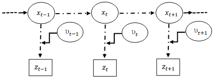
Figure 1: Causality of observations and of the latent variables.

The joint probability density $p(\upsilon_{t},x_{t}|\boldsymbol{z}_{t-1})$ can be expressed recursively as [2, 40],

$$\begin{split}p(\upsilon_{t},x_{t}|\boldsymbol{z}_{t-1})=&\int_{\boldsymbol{\Omega}_{\upsilon,x}^{t-1}}p(\upsilon_{t},x_{t}|\boldsymbol{\upsilon}_{t-1},\boldsymbol{x}_{t-1})\\ &\qquad p(\boldsymbol{\upsilon}_{t-1},\boldsymbol{x}_{t-1}|\boldsymbol{z}_{t-1})\,\mathrm{d}\boldsymbol{\upsilon}_{t-1}d\boldsymbol{x}_{t-1}.\end{split}$$ (9)

Using the Bayes theorem, we can also write,

$$p(\upsilon_{t},x_{t}|\boldsymbol{z}_{t-1})=\frac{p(\boldsymbol{z}_{t-1}|\upsilon_{t},x_{t})\,p(\upsilon_{t},x_{t})}{\int_{\boldsymbol{\Omega}_{\upsilon,x}}p(\boldsymbol{z}_{t-1}|\upsilon_{t},x_{t})\,p(\upsilon_{t},x_{t})\,\mathrm{d}\upsilon_{t}\mathrm{d}x_{t}}.$$ (10)

Since the noises and states are independent, we can further write,

$$p(\boldsymbol{\upsilon}_{t},\boldsymbol{x}_{t})=p(\boldsymbol{\upsilon}_{t})\,p(\boldsymbol{x}_{t})=p(\boldsymbol{x}_{t})\prod_{l=1}^{t}p(\upsilon_{l}).$$ (11)

Note that the presence of noises $\boldsymbol{\upsilon}_{t}$ makes the direct calculation of the posterior computationally intractable.

In order to enable Bayesian variational inference, we need to define or find the variational distributions $q$ which can approximate well the exact distributions $p$. In particular, consider the variational likelihood $q(\boldsymbol{x}_{t}|\boldsymbol{z}_{t})$ and the variational posterior $q(\boldsymbol{\upsilon}_{t},\boldsymbol{x}_{t}|\boldsymbol{z}_{t})$. We have that,

$$q(\boldsymbol{\upsilon}_{t},\boldsymbol{x}_{t}|\boldsymbol{z}_{t})=q(\boldsymbol{x}_{t}|\boldsymbol{z})\,q(\boldsymbol{\upsilon}_{t}|\boldsymbol{z}_{t}).$$ (12)

The variational distributions should be selected, so they maximize the approximation fitness defined as [20],

$$\mathcal{C}_{f}[q]=\int_{\boldsymbol{\Omega}_{\upsilon}^{t}}\mathrm{d}\boldsymbol{\upsilon}_{t}\ q(\boldsymbol{x}_{t}|\boldsymbol{z}_{t})\,q(\boldsymbol{\upsilon}_{t}|\boldsymbol{z}_{t})\ln\frac{p(\boldsymbol{x}_{t}|\boldsymbol{z}_{t})\,p(\boldsymbol{\upsilon}_{t}|\boldsymbol{z}_{t})}{q(\boldsymbol{x}_{t}|\boldsymbol{z}_{t})\,q(\boldsymbol{\upsilon}_{t}|\boldsymbol{z}_{t})}.$$ (13)

The fitness function can be rewritten using the Kullback-Leibler (KL) distance as [22],

$$\mathcal{C}_{f}[q]={\mathrm{E}}\!\left[\ln\frac{p(\boldsymbol{x}_{t}|\boldsymbol{z}_{t})\,p(\boldsymbol{\upsilon}_{t}|\boldsymbol{z}_{t})}{q(\boldsymbol{x}_{t}|\boldsymbol{z}_{t})\,q(\boldsymbol{\upsilon}_{t}|\boldsymbol{z}_{t})}\right]-\mathrm{KL}\left[q(\boldsymbol{\upsilon}_{t})\|p(\boldsymbol{\upsilon}_{t})\right]$$ (14)

where the expectation is taken with respect to the distribution $q(\boldsymbol{\upsilon}_{t},\boldsymbol{x}_{t}|\boldsymbol{z}_{t})$. The expectation represents the mean likelihood, and the second term in (14) is the KL distance between the variational posterior and the true posterior of $\boldsymbol{\upsilon}_{t}$. Furthermore, using Jensen’s inequality, the fitness function can be upper-bounded for any variational distributions $q$ by the marginal likelihood, i.e., [20, 32]

$$\mathcal{C}_{f}[q]\leq\ln p(\boldsymbol{z}_{t}|\boldsymbol{x}_{t})p(\boldsymbol{z}_{t}|\boldsymbol{\upsilon}_{t}).$$ (15)

Therefore, the best variational posterior density must satisfy,

$$\frac{\mathrm{d}}{\mathrm{d}q(\boldsymbol{x}_{t})}\mathcal{C}_{f}[q]=0$$ (16)

subject to $q(\boldsymbol{x}_{t})\geq 0$. Since the states $\boldsymbol{x}_{t}$ are multivariate Gaussian distributed, we get,

$$q(\boldsymbol{x}_{t}|\boldsymbol{z}_{t})\propto\exp\left({\mathrm{E}_{\boldsymbol{\upsilon}_{t}}}\!\left[p(\boldsymbol{z}_{t}|\boldsymbol{x}_{t})p(\boldsymbol{z}_{t}|\boldsymbol{\upsilon}_{t})\right]\right)$$ (17)

where the expectation is calculated with respect to the distribution $q(\boldsymbol{\upsilon}_{t})$. The variational log-likelihood can be then computed as,

$$\ln q(\boldsymbol{x}_{t}|\boldsymbol{z}_{t})\propto\int_{\boldsymbol{\Omega}_{\upsilon}^{t}}\!\!\mathrm{d}\boldsymbol{\upsilon}_{t}\,G(\boldsymbol{\upsilon}_{t}|\alpha,\beta)\ln p(\boldsymbol{z}_{t}|\boldsymbol{x}_{t})p(\boldsymbol{z}_{t}|\boldsymbol{\upsilon}_{t}).$$ (18)

Recall that $\boldsymbol{x}_{t}\sim N(\boldsymbol{x}_{t};\boldsymbol{C}_{\boldsymbol{x}_{t}})$ (i.e., the zero-mean multivariate Gaussian distribution with the covariance matrix $\boldsymbol{C}_{\boldsymbol{x}_{t}}$) and $\boldsymbol{\upsilon}_{t}\sim G(\boldsymbol{\upsilon}_{t};\alpha,\beta)$ (i.e., the product of $t$ gamma distributions). In addition, to obtain the variational distribution $q(\boldsymbol{x}_{t})$, we replace the likelihood distribution $p(\boldsymbol{z}_{t}|\boldsymbol{\upsilon}_{t})$ with the independent Gaussian samples $N(z_{l}|\upsilon_{l})$, and get,

$$\begin{split}\ln q(\boldsymbol{x}_{t}|\boldsymbol{z}_{t})=&\int_{\boldsymbol{\Omega}_{\upsilon}^{t}}\mathrm{d}\boldsymbol{\upsilon}_{t}\ G(\upsilon_{t};\alpha,\beta)\\ &\biggl{\{}\ln N(\boldsymbol{x}_{t};\boldsymbol{C}_{\boldsymbol{x}_{t}})+\ln G(\boldsymbol{\upsilon}_{t};\alpha,\beta)\\ &+\sum_{l=1}^{t}\ln N(z_{l}|\upsilon_{l})\biggr{\}}.\end{split}$$ (19)

This expression can be further manipulated as,

$$\begin{split}\ln q(\boldsymbol{x}_{t}|\boldsymbol{z}_{t})\propto&\ln N(\boldsymbol{x}_{t};\boldsymbol{C}_{\boldsymbol{x}_{t}})\\ &+\sum_{l=1}^{t}\int_{\boldsymbol{\Omega}_{\upsilon}}\!\!\mathrm{d}\upsilon_{l}\,\biggl{\{}\ln G(\upsilon_{l};\alpha,\beta)+\ln N(z_{l}|\upsilon_{l})\biggr{\}}.\end{split}$$ (20)

Using the substitution,

$$ln(z_{l}|x_{l})\propto K^{te}+(z_{l}-x_{l})^{2}{\mathrm{E}}\!\left[\upsilon_{l}\right]$$ (21)

for some constant $K$, we can simplify the variational log-distribution as,

$$\begin{split}\ln q(\boldsymbol{x}_{t}|\boldsymbol{z}_{t})\propto&\ln N(\boldsymbol{x}_{t};\boldsymbol{C}_{\boldsymbol{x}_{t}})\\ &+\sum_{l=1}^{t}(z_{l}-x_{l})^{2}{\mathrm{E}}\!\left[\upsilon_{l}\right]+\ln K^{-te}.\end{split}$$ (22)

Consequently, the variational distribution becomes,

$$q(\boldsymbol{x}_{t}|\boldsymbol{z}_{t})\propto K^{-te}\,N(\boldsymbol{x}_{t};\boldsymbol{C}_{\boldsymbol{x}_{t}})\exp\!\left\{\sum_{l=1}^{t}(z_{l}-x_{l})^{2}{\mathrm{E}}\!\left[\upsilon_{l}\right]\right\}.$$ (23)

This variational distribution can be used in the SMC-SISR method to generate samples representing the posterior distribution $p(x_{t}|\boldsymbol{x}_{t-1},\boldsymbol{z}_{1:t})$.

3 Variational Bayesian estimation

We adopt a non-parametric inference strategy involving random sampling. In particular, assuming the distributions derived in the previous section, we modify the SMC-SISR estimator to fit our scenario of estimating a hidden ARMA random process from non-linear and noisy observations. The SMC-SISR estimator represents the posterior density by a set of evolving random samples and the associated weights. The efficiency of this estimator is strongly influenced by the choice of the sampling distribution [29, 30]. In many cases, using the prior distribution as the sampling distribution can be a sensible choice [10].

Consider the set of $N$ particles and their weights, i.e., $\left\{x_{t}^{(i)},w_{t}^{(i)}\right\}_{i=1}^{N}$, evolving over a discrete time $t$ to represent the posterior distribution $p(\boldsymbol{x}_{t}|\boldsymbol{z}_{t})$. The weights are periodically normalized, so that, $\sum_{i=1}^{N}w_{t}^{(i)}=1$ at all time instances. The posterior density at time $t$ is approximated as,

$$p(\boldsymbol{x}_{t}|\boldsymbol{z}_{t})\approx\sum_{i=1}^{N}w_{t}^{(i)}\delta(\boldsymbol{x}_{t}-\boldsymbol{x}_{t}^{(i)}).$$ (24)

Thus, the distances $\delta$ between the $i$-th particle $\boldsymbol{x}_{t}^{(i)}$ and the true latent states $\boldsymbol{x}_{t}$ are weighted by the coefficients $w_{t}^{(i)}$. Here, we assume that particles are generated from the proposal density used in the importance sampling of the SISR estimator. The proposal distribution can be represented recursively as,

$$\pi(x_{t}|\boldsymbol{x}_{t-1},\boldsymbol{z}_{t})=\pi(x_{1}|z_{1})\prod_{l=2}^{t}\pi(x_{l}|\boldsymbol{x}_{l-1},\boldsymbol{z}_{l}).$$ (25)

Consequently, the weight for the latent state $x_{t}$ required in designing the importance sampling is calculated as the ratio of the posterior and the proposal distributions, i.e.,

$$w(x_{t})=\frac{p(x_{t}|\boldsymbol{x}_{t-1},\boldsymbol{z}_{t})}{\pi(x_{t}|\boldsymbol{x}_{t-1},\boldsymbol{z}_{t})}.$$ (26)

It is, however, more convenient to calculate the weights recursively as,

$$w(x_{t})=w(x_{t-1})\,\frac{p(z_{t}|x_{t})p(x_{t}|\boldsymbol{x}_{t-1})}{\pi(x_{t}|\boldsymbol{x}_{t-1},\boldsymbol{z}_{t})}.$$ (27)

The weights are then normalized as,

$$\tilde{w}(x_{t}^{(i)})=\frac{w(x_{t}^{(i)})\frac{p(z_{t}|x_{t}^{(i)})p(x_{t}^{(i)}|\boldsymbol{x}_{t-1}^{(i)})}{\pi(x_{t}^{(i)}|\boldsymbol{x}_{t-1}^{(i)},\boldsymbol{z}_{t})}}{\sum_{i=1}^{N}w(x_{t}^{(i)})\frac{p(z_{t}|x_{t}^{(i)})p(x_{t}^{(i)}|\boldsymbol{x}_{t-1}^{(i)})}{\pi(x_{t}^{(i)}|\boldsymbol{x}_{t-1}^{(i)},\boldsymbol{z}_{t})}}.$$ (28)

Since in our case, the proposal distribution is equal to the prior distribution, the normalized weights can be approximated as,

$$\tilde{w}(x_{t}^{(i)})=w(x_{t-1}^{(i)})\,p(z_{t}|x_{t}^{(i)}).$$ (29)

Furthermore, to resolve the degeneracy of samples which occurs with all sequential sampling methods, the resampling step at every iteration discards the particles with small weights, and replace them with new particles having larger weights [13]. More specifically, at each time step, the $i$-th particle is replaced with the probability $1-\tilde{w}(x_{t}^{(i)})$ by a new particle. If the particle is replaced, the new particle is assigned the weight equal to the arithmetic mean of the other particles [27, 26]. Selecting the proper particle weight is important to yield an unbiased SMC estimation of the marginal likelihood, and to maintain the particle diversity.

4 Numerical examples

Numerical examples are used to validate and evaluate the estimation accuracy of the devised SMC-SISR estimator utilizing the derived distributions and the sample weights. The examples assume stochastic log-volatility state-space model from [10]. The volatility model has many applications in finance and econometrics where it is used to assess the risks [28]. Mathematically, the stochastic volatility model is an example of the non-linear ARMA model defined in (1). The volatility model generates the zero-mean stationary fractional Gaussian states $x_{t}$ with the observations described as,

$$z_{t}=\upsilon_{t}\ \mathrm{e}^{x_{t}/2}.$$ (30)

Provided that $\hat{x}_{t}$ denotes the estimate of the true state $x_{t}$, the estimation accuracy can be evaluated as the root mean-square error (RMSE) defined as,

$$\mathrm{RMSE}_{t}=\sqrt{\frac{1}{t}\sum_{i=1}^{t}(x_{i}-\hat{x}_{i})^{2}}.$$

The ARMA models and their parameters used in our numerical experiments are summarized in Table 1. The variance of the innovation process $u_{t}$ is set to unity, i.e., $\sigma_{u}^{2}=1$. The gamma distribution of the IID observation noises has the parameters $\alpha=1/2$ and $\beta=1$. The number of particles tracked by the SMC-SISR estimator is $N=1000$. We did not observe any noticeable improvement in the estimation accuracy for larger values of $N$. However, it is possible to fine tune the effective number of particles to be less than this value. More importantly, our numerical experiments showed that the estimation accuracy of the low-order ARMA models is comparable with the estimation accuracy of the higher-order ARMA models.

Table 1: The ARMA models used in simulations presented in Figures 2–7.

Figure	Model	$\phi_{1}$	$\phi_{2}$	$\varphi_{1}$	$\varphi_{2}$	$H$
2	ARMA$(1,1)$	$0.85$	-	$0.8$	-	$0.7$
3	ARMA$(2,1)$	$0.49$	$0.49$	$0.8$	-	$0.8$
4	AR$(1)$	$0.6$	-	-	-	$0.7$
5	MA$(1)$	-	-	$0.5$	-	$0.7$
6	AR$(2)$	$0.49$	$0.45$	-	-	$0.8$
7	MA$(2)$	-	-	$0.49$	$0.47$	$0.8$

The simulation results are presented in Figures 2 – 7. Each figure consists of two parts. The upper plot compares a sample realization of the true latent state sequence $x_{t}$ with the estimated sequence $\hat{x}_{t}$. The lower plot then shows the corresponding RMSE of the estimated sequence.

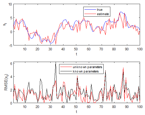
Figure 2: The sample latent sequence $x_{t}$ and its estimate $\hat{x}_{t}$ for the ARMA$(1,1)$ model and the corresponding RMSE.

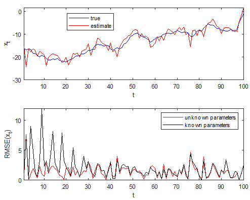
Figure 3: The sample latent sequence $x_{t}$ and its estimate $\hat{x}_{t}$ for the ARMA$(2,1)$ model and the corresponding RMSE.

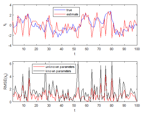
Figure 4: The sample latent sequence $x_{t}$ and its estimate $\hat{x}_{t}$ for the AR$(1)$ model and the corresponding RMSE.

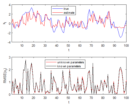
Figure 5: The sample latent sequence $x_{t}$ and its estimate $\hat{x}_{t}$ for the MA$(1)$ model and the corresponding RMSE.

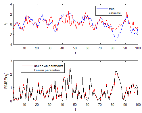
Figure 6: The sample latent sequence $x_{t}$ and its estimate $\hat{x}_{t}$ for the AR$(2)$ model and the corresponding RMSE.

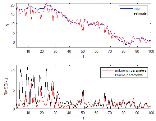
Figure 7: The sample latent sequence $x_{t}$ and its estimate $\hat{x}_{t}$ for the MA$(2)$ model and the corresponding RMSE.

4.1 Gene expression time series example

We now investigate more complex as well as more practical problem of inferring missing values in the gene expression time series. The inference is performed by the SMC-SISR estimator developed in the previous sections. The missing data in biological experiments may be caused by unexpectedly large measurement errors (outliers), or due to other intermittent problems in the experimental measurements. The gene expression data are vital for reconstructing gene expression networks [43]. More importantly, simple deterministic interpolation to replace the missing data values did not provide satisfactory results [6].

The gene expression data can be modeled by a vector autoregressive (VAR) model [16, 37]. We can directly employ the SMC-SISR estimator instead of first estimating the parameters of this model, In particular, the sequence $\boldsymbol{x}_{t}$ of the gene expression time series can be modeled recursively by the $k$-order VAR model, i.e., let,

$$\boldsymbol{x}_{t}=\sum_{i=1}^{k}\boldsymbol{W}_{i}\,\boldsymbol{x}_{t-i}+\boldsymbol{u}_{t}$$ (31)

where $n$ is the number of genes (i.e., the sample size of the time series data observed at each time instant), the $(n\times n)$ matrices $\boldsymbol{W}_{i}$ represent the model parameters, and $\boldsymbol{u}_{t}$ is a $(n\times 1)$ vector of Gaussian innovations which are zero mean and uncorrelated. The observations are modeled as in (30).

The actual gene expression data for the Hela cell were obtained from the supplementary material provided in [41]. The data provide measurements at $16$ time instances separated by one hour over $3$ cell cycles, so the total number of data points is $48$. The data for the genes 7p21 and p53 were selected as two representative examples. Rather than fitting the model parameters to the model described by (30) and (31), we can use the SMC-SISR estimator with $1000$ particles to track the most probable counts of the gene produced in the cell. The actual and predicted counts of the two genes are shown in Figure 8 and 9, respectively. We can observe that the random sampling model follows the expression data reasonably well, and the estimation error is likely sufficient for many biological applications.

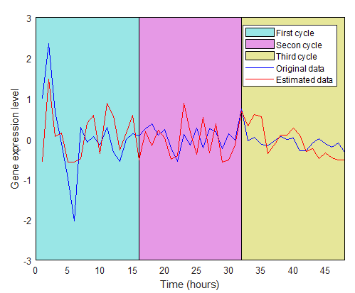
Figure 8: Tracking the expression data for the 7p21 gene in the Hela cell using the SMC-SISR estimator.

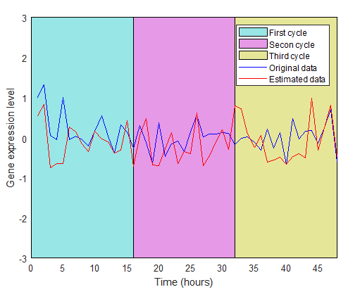
Figure 9: Tracking the expression data for the p53 gene in the Hela cell using the SMC-SISR estimator.

5 Discussion

Considering numerical experiments and other results presented in this paper, we can conclude that the latent time series can be estimated with good accuracy from non-linear and noisy observations even if the parameters of the underlying model are not known. The unknown parameters include the ARMA model coefficients as well as the parameters describing the input innovation process such as the variance, and the autocorrelation. Such assumption may be important especially in situations when all or some of the model parameters cannot be easily estimated. For example, the parameters may be time varying and even non-stationary [7, 34]. In such case, the SMC estimator may not be able to track the parameter variations. However, if the model parameters vary sufficiently fast, the SMC estimator can instead follow possibly time-varying mean values of the model parameters representing slowly changing random processes.

Provided that the latent states are non-negative integers or positive real values, the measurement noise is generally dependent on the latent state values in order to satisfy this constraint. The correlations between the states and the measurement noises would substantially complicate the state inference. In this paper, we assumed that the measurement noises are gamma distributed and IID, so it does not violate the non-negativity constraint of the latent state values. Furthermore, the computational complexity of calculating the posterior of latent states dictates the use of variational Bayesian inference or other methods for approximating the posterior distribution [17, 9].

The performance of the SMC-SISR estimator was shown to be good for several low-order ARMA models. There are many practical applications where the inference of latent states from observations is important. For instance, such inferences are used to reconstruct the state space models of dynamic systems [11, 42], or as illustrated in this paper, we can infer missing values in the time series data. The gene expression data are an example of the multi-dimensional time series where the expressions of multiple genes are measured in parallel at discrete time instances. In general, gene expression data are useful to reconstruct gene reaction networks, and to elucidate the properties and understanding of genetic circuits [3, 4, 5].

6 Conclusion

The SMC sampling estimators are usually used to perform variational Bayesian inference in order to reduce the computational complexity by approximating the posterior distribution. More importantly, these estimators such as the SMC-SISR estimator adopted in this paper can be effective in estimating the hidden random processes from non-linear and noisy observations, even if the parameters of the underlying state space model are not known. The numerical results indicate that the SMC-SISR estimator achieves good estimation accuracy, especially for the low-order ARMA models, and this estimator is also unbiased.

There are many practical situations where the inference problem considered in this paper is encountered. One such problem was briefly investigated to demonstrate the performance of the SMC-SISR estimator for the time series data with multiple observations at each time instant to infer the missing values. Future work will consider different non-linearity observation functions and noise distributions, and the inference problem for the data models with time-varying random parameters. In this latter case, the SMC sampling estimators may track changes in the hidden state statistics, or these statistics can be averaged out from the likelihood function or from the posterior distribution.

References

- [1] L. Acerbi. Variational Bayesian Monte Carlo. In Advances in Neural Infor. Processing Systems, pages 8213–8223, 2018.
- [2] K. Atitey and Y. Cang. A novel prediction algorithm in Gaussian-mixture probability hypothesis density filter for target tracking. In International Conference on Image and Graphics, pages 373–393, 2015.
- [3] K. Atitey, P. Loskot, and P. Rees. Determining the transcription rates yielding steady-state production of mRNA in the lac genetic switch of Escherichia coli. Journal of Computational Biology, 25(9):1023–1039, 2018.
- [4] K. Atitey, P. Loskot, and P. Rees. Inferring distributions from observed mRNA and protein copy counts in genetic circuits. Biomedical Physics & Engineering Express, 2018.
- [5] K. Atitey, P. Loskot, and P. Rees. Elucidating effects of reaction rates on dynamics of the lac circuit in Escherichia coli. Biosystems, 175:1–10, 2019.
- [6] Z. Bar-Joseph, G. K. Gerber, D. K. Gifford, T. S. Jaakkola, and I. Simon. Continuous representations of time-series gene expression data. Journal of Computational Biology, 10(3-4):341–356, 2003.
- [7] A. Bibi. Evolutionary transfer functions of bilinear processes with time-varying coefficients. Computers & Mathematics with Applications, 52(3-4):331–338, 2006.
- [8] D. M. Blei, A. Kucukelbir, and J. D. McAuliffe. Variational inference: A review for statisticians. Journal of the American Statistical Association, 112(518):859–877, 2017.
- [9] C. Bracegirdle. Inference in Bayesian Time-Series Models. PhD thesis, University College London, UK, 2013.
- [10] R. Casarin. Bayesian Monte Carlo filtering for stochastic volatility models. Technical report, Cahier du CEREMADE No. 0415. Available at SSRN: https://ssrn.com/abstract=739766 or http://dx.doi.org/10.2139/ssrn.739766, 2004.
- [11] M. Casdagli, S. Eubank, J. D. Farmer, and J. Gibson. State space reconstruction in the presence of noise. Physica D: Nonlinear Phenomena, 51(1-3):52–98, 1991.
- [12] J. Daunizeau, K. J. Friston, and S. J. Kiebel. Variational Bayesian identification and prediction of stochastic nonlinear dynamic causal models. Physica D: nonlinear phenomena, 238(21):2089–2118, 2009.
- [13] A. Doucet and A. M. Johansen. A tutorial on particle filtering and smoothing: Fifteen years later. Handbook of nonlinear filtering, 12(656-704):3, 2009.
- [14] S. Durlauf and L. Blume. Macroeconometrics and time series analysis. Springer, 2016.
- [15] C. Elster, K. Klauenberg, M. Walzel, G. Wübbeler, P. Harris, M. Cox, C. Matthews, I. Smith, L. Wright, A. Allard, et al. A guide to Bayesian inference for regression problems. EMRP Project NEW04 “Novel Mathematical and Statistical Approaches to Uncertainty Evaluation”, 2015.
- [16] A. Fujita et al. Modeling gene expression regulatory networks with the sparse vector autoregressive model. BMC Systems Biology, 1(1):39, 2007.
- [17] M. J. Beal et al. Variational algorithms for approximate Bayesian inference. University of London, 2003.
- [18] B. C. Geiger, T. Petrov, G. Kubin, and H. Koeppl. Optimal Kullback–Leibler aggregation via information bottleneck. IEEE Trans. Aut. Control, 60(4):1010–1022, 2015.
- [19] P. J. Green, K. Łatuszyński, M. Pereyra, and C. P. Robert. Bayesian computation: A summary of the current state, and samples backwards and forwards. Statistics and Computing, 25(4):835–862, 2015.
- [20] Attias Hagai. A variational Baysian framework for graphical models. In Advances in Neural Information Processing Systems, pages 209–215, 2000.
- [21] J. Helske. Computational efficiency comparison of MCMC algorithms for non-Gaussian state space models. Technical Report, 2017.
- [22] Zhaolin Hu and L Jeff Hong. Kullback-Leibler divergence constrained distributionally robust optimization. Optimization Online, 2013.
- [23] Y. Kamarianakis, P. Prastacos, et al. Spatial time series modeling: A review of the proposed methodologies. The Regional Economics Applications Laboratory, 2003.
- [24] A. Leon-Garcia. Probability, Statistics, and Random Processes for Electrical Engineering. Pearson Education, 2017.
- [25] C. Liu, S. C. Hoi, P. Zhao, and J. Sun. Online ARIMA algorithms for time series prediction. In Thirtieth AAAI Conference on Artificial Intelligence, 2016.
- [26] L. Martino, V. Elvira, and G. Camps-Valls. Group importance sampling for particle filtering and MCMC. Digital Signal Processing, 82:133–151, November 2018.
- [27] L. Martino, V. Elvira, and F. Louzada. Weighting a resampled particle in sequential Monte Carlo. In IEEE SSP, 2016.
- [28] Z. Men. Bayesian inference for stochastic volatility models. PhD thesis, University of Waterloo, 2012.
- [29] L. Mihaylova, P. Brasnett, A. Achim, D. Bull, and N. Canagarajah. Particle filtering with alpha-stable distributions. In IEEE/SP 13th Workshop on Statistical Signal Processing, 2005, pages 381–386, 2005.
- [30] L. Mihaylova, A. Y. Carmi, F. Septier, A. Gning, S. K. Pang, and S. Godsill. Overview of Bayesian sequential Monte Carlo methods for group and extended object tracking. Digital Signal Processing, 25:1–16, 2014.
- [31] T. C. Mills. Time series techniques for economists. Cambridge University Press, 1991.
- [32] Radford M Neal and Geoffrey E Hinton. A view of the EM algorithm that justifies incremental, sparse, and other variants. In Learning in Graphical Models, pages 355–368. Springer, 1998.
- [33] F. J Nogales and A. J. Conejo. Electricity price forecasting through transfer function models. Journal of the Operational Research Society, 57(4):350–356, 2006.
- [34] R. Pintelon and J. Schoukens. Time series analysis in the frequency domain. IEEE Transactions on Signal Processing, 47(1):206–210, 1999.
- [35] T. Raiko, H. Valpola, M. Harva, and J. Karhunen. Building blocks for variational Bayesian learning of latent variable models. J. Mach. Learning Research, 8(Jan):155–201, 2007.
- [36] A. Román-Rosales, E. García-Villa, L. Herrera, P. Gariglio, and J. Díaz-Chávez. Mutant p53 gain of function induces HER2 over-expression in cancer cells. BMC Cancer, 18(1):709, 2018.
- [37] G. H. Tam, Y. S. Hung, and C. Chang. Synthetic time series resembling human (HeLa) cell-cycle gene expression data and application to gene regulatory network discovery. In International Conference on Intelligent Human-Machine Systems and Cybernetics, volume 2, pages 538–541, 2013.
- [38] R. S. Tsay. Analysis of Financial Time Series, volume 543. John wiley & sons, 2005.
- [39] I. Urteaga, M. F Bugallo, and P. M. Djurić. Sequential Monte Carlo for inference of latent ARMA time-series with innovations correlated in time. EURASIP Journal on Advances in Signal Processing, 2017: 84, 2017.
- [40] B-N Vo and W-K Ma. The Gaussian mixture probability hypothesis density filter. IEEE Transactions on Signal Processing, 54(11):4091–4104, 2006.
- [41] M. L. Whitfield, G. Sherlock, A. J. Saldanha, J. I. Murray, C. A. Ball, K. E. Alexander, J. C. Matese, C. M. Perou, M. M. Hurt, P. O. Brown, et al. Identification of genes periodically expressed in the human cell cycle and their expression in tumors. Molecular Biology of the Cell, 13(6):1977–2000, 2002.
- [42] X. Yang, X. Zheng, and L. Lv. A spatiotemporal model of land use change based on ant colony optimization, Markov chain and cellular automata. Ecological Modelling, 233:11–19, 2012.
- [43] S. Yao, S. Yoo, and D. Yu. Prior knowledge driven granger causality analysis on gene regulatory network discovery. BMC Bioinformatics, 16(1):273, 2015.