Surfaces and hypersurfaces as the joint spectrum of matrices

Abstract.

The Clifford spectrum is an elegant way to define the joint spectrum of several Hermitian operators. While it has been know that for examples as small as three $2$-by-$2$ matrices the Clifford spectrum can be a two-dimensional manifold, few concrete examples have been investigated. Our main goal is to generate examples of the Clifford spectrum of three or four matrices where, with the assistance of a computer algebra package, we can calculate the Clifford spectrum.

1. Introduction

The Clifford spectrum is one way extend the concept of joint spectrum of commuting matrices to work for noncommuting operators. We are only interested in Hermitian matrices as in the back of our minds we envision applications to quantum physics and string theory. Given $(X_{1},\dots,X_{d})$, where the $X_{j}$ are all $n$-by-$n$ Hermitian matrices, we define a Dirac-type operator

$$L(X_{1},\dots,X_{d})=\sum X_{j}\otimes\gamma_{j}$$

where the $\gamma_{j}$ are $d$ matrices that satisfy the Clifford relations

(1.1) $$\begin{aligned} \gamma_{j}^{*}&=\gamma_{j}\quad(\forall j)\\ \gamma_{j}^{2}&=I\quad(\forall j)\\ \gamma_{j}\gamma_{k}&=-\gamma_{k}\gamma_{j}\quad(j\neq k)\end{aligned}.$$

We can use $L(X_{1},\dots,X_{d})$ to determine only if $\boldsymbol{0}$ is in the Clifford spectrum. To find the full spectrum, we shift the matrices by scalars, and define

$$L_{\boldsymbol{\lambda}}(X_{1},\dots,X_{d}) =L(X_{1}-\lambda_{1},\dots,X_{d}-\lambda_{d})$$

$$=\sum\left(X_{j}-\lambda_{j}\right)\otimes\gamma_{j}.$$

Due to many clashes of terminology between mathematics and physics, it seems now prudent, as discussed in [7], to call $L_{\boldsymbol{\lambda}}$ the spectral localizer of the $d$-tuple $(X_{1},\dots,X_{d})$.

Definition 1.1.

The Clifford spectrum of $d$-tuple $(X_{1},\dots,X_{d})$ of Hermitian matrices is the set of $\lambda$ in $\mathbb{R}^{d}$ such that $L_{\boldsymbol{\lambda}}(X_{1},\dots,X_{d})$ is singular. This is denoted $\Lambda(X_{1},\dots,X_{d})$.

Remark 1.2.

This definition works for Hermitian operators, even when unbounded. We will focus on the matrix case, except in a few comments and examples.

It was Kisil [6] who noticed that the Clifford spectrum equals the Taylor spectrum in the case where the $X_{j}$ all commute with each other. In the case of finite matrices, a singular localizer at $\boldsymbol{\lambda}$ implies there is a joint eivenvector with eigenvalues the components of $\boldsymbol{\lambda}$, and this is exactly what any form of joint spectrum should mean for commuting finite matrices. We will see a more general result in §2, where it is shown that for almost commuting matrices we can associate to points in the Clifford spectrum vectors with small variation with respect to each $X_{j}$.

Kisil also used the theory of monogenic functions to prove that the Clifford spectrum is always nonempty, and indeed compact. However, it does not have to be a finite set when computed for finite matrices that don’t commute.

In string theory, the Clifford spectrum is used, but tends to be called the “emergent geometry” [1], or the “set of probe points” [12] etc. In that context, the Clifford spectrum consists of all the locations where a fermionic probe of a D brane can lead to low energy resonance.

For some calculations we will look at the square of the localizer. It is important to note that the square of this Dirac-type matrix is not exactly the corresponding Laplace-type matrix. Indeed, one can calculate [9] that

(1.2) $$\left(L_{\boldsymbol{\lambda}}(X_{1},\dots,X_{d})\right)^{2}=\sum_{j=1}^{d}\left(X_{j}-\lambda_{j}\right)^{2}\otimes I+\sum_{j<k}[X_{j},X_{k}]\otimes\gamma_{j}\gamma_{k}.$$

Why not use directly a Laplace-type operator to define a spectrum? This will be correct in the commuting case.

Definition 1.3.

The Laplace spectrum of Hermitian $d$-tuple $(X_{1},\dots,X_{d})$ is the set of $\lambda$ in $\mathbb{R}^{d}$ such that

$$\sum_{j=1}^{d}\left(X_{j}-\lambda_{j}\right)^{2}$$

is singular.

The Laplace spectrum is used in string theory [12]. We will see it has a flaw that keeps it out of general use. In some cases, when the commutators are small, one might be able to prove that the Laplace spectrum is a decent approximation of the Clifford spectrum.

An issue with the Clifford spectrum is that it is very hard to work examples by hand. Looking hard at the math and string theory literature, we find a only a handful of explicit examples where the Clifford spectrum is known. Indeed, Schneiderbauer and Steinacker [12], and also Sykora [13], use a computer algebra package for many fuzzy geometry calculations. We are taking on a similar challenge, using a computer algebra package to find more examples.

We will primarily use a generalized characteristic polynomial to calculate the Clifford spectrum of various examples. The generalized characteristic polynomial probably first appeared in work by Berenstein, Dzienkowski and Lashof-Regas [2].

Definition 1.4.

The characteristic polynomial of the $d$-tuple $(X_{1},\dots,X_{d})$ is the polynomial, in real variables $\lambda_{1}\dots,\lambda_{d}$,

$$\boldsymbol{\lambda}\mapsto\det(L_{\boldsymbol{\lambda}}(X_{1},\dots,X_{d}))$$

which we denote $\mathrm{char}(X_{1},\dots,X_{d})$.

The equation $\mathrm{char}(X_{1},\dots,X_{d})=0$ determines the Clifford spectrum. This can become a polynomial with many monomials in many variable even in rather modest examples. Hence the need for a computer assist and an experimental approach.

Some of the complexity from increasing $d$, the number of matrices, comes from the fact that the $\gamma_{j}$ get bigger. It is best to use an irreducible representation of (1.1), which means that each $\gamma$ is $g$-by-$g$ for

$$g=2^{\lfloor d/2\rfloor}$$

as one can see from [11], for example. The wrong value for $g$ was used in [9, §1] and so the estimates there were not correct as stated. See Section 2.

Section 2 discusses the variance of joint approximate eigenvalues. Section 3 discusses the cases of one or two matrices (or operators) where the Clifford spectrum agrees with the ordinary single-operator spectrum. Section 4 looks at the case of three matrices, where the Clifford spectrum can be a surface. This is where we have the most examples, as surfaces in three space are easy to display. Section 5 looks as the case of four matrices, where the calculations and visualization become harder. Section 6 looks are variations on the localizer and index that assist with plotting and proving the stability of the Clifford spectrum. Many of these examples in Section 4 and the discussion of the archetypal polynomial are from the thesis of DeBonis [4].

We will use mathematical notation throughout. Most importantly, Hermitian matrices are those for which $X^{*}=X$, and so complex conjugation is indicated by $X^{*}$. In several places we will focus on unit vectors, so have in mind states of a quantum system. Since the word state means something different in operator algebras, for this we stick the the neutral terminology.

The convention we prefer for identifying a tensor product of matrices with a larger matrix is the one such that

$$A\otimes\begin{pmatrix}a&b\\ c&d\end{pmatrix}=\begin{pmatrix}aA&bA\\ cA&dA\end{pmatrix}$$

and this is opposite of the convention used by the KroneckerProduct operation in Mathematica.

2. Bounds on variance

Suppose $\mathbf{v}$ is a unit vector and $X$ is a Hermitian matrix. Two important quantities when considering quantum measurement are the expection value of $X$ with respect to $\mathbf{v}$

$$\textnormal{E}(X)_{\mathbf{v}}=\langle X\mathbf{v},\mathbf{v}\rangle$$

and the variance of $X$ with respect to $\mathbf{v}$

$$\textnormal{Var}(X)_{\mathbf{v}}=\langle X^{2}\mathbf{v},\mathbf{v}\rangle-\langle X\mathbf{v},\mathbf{v}\rangle^{2}.$$

For any scalar $\lambda$ we have

$$\left\langle(X-\lambda)^{2}\mathbf{v},\mathbf{v}\right\rangle=\left\langle X^{2}\mathbf{v},\mathbf{v}\right\rangle-2\lambda\left\langle X\mathbf{v},\mathbf{v}\right\rangle+\lambda^{2}$$

and

$$\left\langle(X-\lambda)\mathbf{v},\mathbf{v}\right\rangle^{2}=\left\langle X\mathbf{v},\mathbf{v}\right\rangle^{2}-2\lambda\left\langle X\mathbf{v},\mathbf{v}\right\rangle+\lambda^{2}$$

so we see that

(2.1) $$\textnormal{Var}(X-\lambda)_{\mathbf{v}}=\textnormal{Var}(X)_{\mathbf{v}}.$$

On the other hand,

(2.2) $$\textnormal{E}(X-\lambda)_{\mathbf{v}}=\textnormal{E}(X)_{\mathbf{v}}-\lambda.$$

If the $\textnormal{Var}(X)_{\mathbf{v}}=0$ then $\mathbf{v}$ is an eigenvector for $X$ for eigenvalue $\textnormal{E}(X)_{\mathbf{v}}$.

When attempting joint measurement, for observables $X_{1},\dots,X_{d}$, one confronts often the impossibility of finding any unit vector $\mathbf{v}$ that is simultaneously an eigenvector for all the observables. There are many lower bounds on the variances that make this more precise, such as the Robertson–Schrödinger relation bounding the product of the variance of two observables. A more recent example of such a lower bound, due to Chen and Fei [3], gives lower bounds on the sum of $d$ variances.

We look here at upper bounds on the sum of variances. Specifically, we will derive an estimate on how small we can make the variances for if we choose certain unit vectors that are related to points in the Clifford spectrum.

Lemma 2.1.

Suppose $X_{1},\dots,X_{d}$ are Hermitian, $n$-by-$n$ matrices and $\boldsymbol{\lambda}$ is in $\Lambda(X_{1},\dots,X_{d})$. Then there is a unit vector $\mathbf{w}$ in $\mathbb{R}^{n}$ such that

$$\sum\left\langle\left(X_{j}-\lambda_{j}\right)^{2}\mathbf{w},\mathbf{w}\right\rangle\leq g\sum_{j<k}\left\|\left[X_{j},X_{k}\right]\right\|$$

for $g=2^{\lfloor d/2\rfloor}$.

Proof.

Since shifting the $X_{j}$ by $\lambda_{j}$ has no effect on the commutators, we can reduce to the case of $\boldsymbol{\lambda}=\boldsymbol{0}$. Assume then that $\bf{0}$ is in the Clifford spectrum of $X_{1},\dots,X_{d}$. Then there is a vector $\mathbf{z}$ in $\mathbb{R}^{gn}$ such that

(2.3) $$L_{\bf{0}}(X_{1},\cdots,X_{n})\mathbf{z}=0$$

One might be tempted to diagonalize $L_{\bf{0}}(X_{1},\cdots,X_{d})$ so that $\boldsymbol{z}$ can be written down as a column vector with only one single non-zero entry. This, however, would not be the best move: if we change coordinate system, then $X_{1}\otimes\gamma_{1}+\cdots+X_{n}\otimes\gamma_{d}$ would no longer be written in a block form and, therefore, we would no longer be able to isolate $X_{j}$ and use some of its properties. Therefore, we refrain from diagonalizing and write $\mathbf{z}$ as

(2.4) $$\mathbf{z}=\begin{bmatrix}\mathbf{z}_{1}\\ \vdots\\ \mathbf{z}_{g}\end{bmatrix}$$

where $\mathbf{z}_{k}\in\mathbb{R}^{n}$ for all $k\in\{1,\cdots,g\}$. From (2.3) we obtain $\left(L_{\bf{0}}(X_{1},\cdots,X_{n})\right)^{2}\mathbf{z}=0$. Now (1.2) tells us

$$\sum_{j}(X_{j}^{2}\otimes I_{g})\mathbf{z}=-\sum_{j<k}([X_{j},X_{k}]\otimes(\gamma_{j}\gamma_{k}))\mathbf{z}$$

and therefore

$$\left\|\sum_{j}X_{j}^{2}\mathbf{z}_{r}\right\|\leq\sum_{j<k}\|[X_{j},X_{k}]\|$$

for every $r$. Now we select $r$ in such a way that it maximizes $\|\mathbf{z}_{r}\|$ and set

$$\mathbf{w}=\frac{1}{\|\mathbf{z}_{r}\|}\mathbf{z}_{r}.$$

Thus,

$$1=\|\mathbf{z}\|^{2}=\sum_{j=1}^{g}\|\boldsymbol{z}_{j}\|^{2}\leq g\|\mathbf{z}_{r}\|^{2}$$

and, therefore, $\|\mathbf{z}_{r}\|\geq 1/\sqrt{g}$. We can now perform the following calculation:

$$\sum\left\langle X_{j}^{2}\mathbf{w},\mathbf{w}\right\rangle =\left\langle\sum X_{j}^{2}\mathbf{w},\mathbf{w}\right\rangle$$

$$\leq g\left\langle\sum X_{j}^{2}\mathbf{z}_{r},\mathbf{z}_{r}\right\rangle$$

$$\leq g\sum_{j<k}\|[X_{j},X_{k}]\|.$$

∎

Theorem 2.2.

Suppose $X_{1},\dots,X_{d}$ are Hermitian, $n$-by-$n$ matrices and $\boldsymbol{\lambda}$ is in $\Lambda(X_{1},\dots,X_{d})$. Then there is a unit vector $\mathbf{w}$ in $\mathbb{R}^{n}$ such that

$$\sum_{j=1}^{d}\textnormal{Var}(X_{j})_{\mathbf{w}}+\left|\textnormal{E}(X_{j})_{\mathbf{w}}-\lambda_{j}\right|^{2}\leq g\sum_{j<k}\left\|\left[X_{j},X_{k}\right]\right\|$$

for $g=2^{\lfloor d/2\rfloor}$.

Proof.

By (2.1) and (2.2) we can again assume, without loss of generality, that $\boldsymbol{\lambda}=\mathbf{0}$. By Lemma 2.1 there exists a unit vector $\mathbf{w}$ such that

$$\sum\left\langle X_{j}^{2}\mathbf{w},\mathbf{w}\right\rangle\leq g\sum_{j<k}\left\|\left[X_{j},X_{k}\right]\right\|.$$

For any Hermitian matrix $X$ and unit vector $\mathbf{v}$ we have

$$\left\langle X^{2}\mathbf{v},\mathbf{v}\right\rangle=\textnormal{Var}(X)_{\mathbf{v}}+\left(\textnormal{E}(X)_{\mathbf{v}}\right)^{2}$$

so in this special case we have

$$\sum\left(\textnormal{Var}(X_{j})_{\mathbf{w}}+\left(\textnormal{E}(X_{j})_{\mathbf{w}}\right)^{2}\right)\leq g\sum_{j<k}\left\|\left[X_{j},X_{k}\right]\right\|.$$

∎

For larger matrices, it will be difficult to determine the exact location of the Clifford spectrum. A more practical approach is to find $\mathbf{\lambda}$ that are in the (Clifford) $\epsilon$-pseudospectrum of $X_{1},\dots,X_{d}$, denoted $\Lambda_{\epsilon}(X_{1},\dots,X_{d})$ as defined in [9]. By definition, $\mathbf{\lambda}$ is in $\Lambda_{\epsilon}(X_{1},\dots,X_{d})$ whenever

(2.5) $$\|(L_{\boldsymbol{\lambda}}(X_{1},\cdots,X_{n})^{-1}\|^{-1}\leq\epsilon.$$

In this paper, we will not use the function

$$\boldsymbol{\lambda}\mapsto\|(L_{\boldsymbol{\lambda}}(X_{1},\cdots,X_{n})^{-1}\|^{-1}$$

to estimate the Clifford spectrum. Notice, however, that (2.5) is equivalent to the existence of a unit vector $\mathbf{\lambda}$ such that

(2.6) $$L_{\boldsymbol{\lambda}}(X_{1},\cdots,X_{n})\mathbf{z}\leq\epsilon.$$

This can be proven easily if one considers a unitary diagonalization of the localizer, which is itself Hermitian.

It is rather easy to compute a unit vector that satisfies (2.6) and such vectors can in interesting, as we now show.

Lemma 2.3.

Suppose $X_{1},\dots,X_{d}$ are Hermitian, $n$-by-$n$ matrices and there is a vector $\mathbf{z}$ in $\mathbb{R}^{gn}$ such that (2.6) holds for some $\epsilon\geq 0$. Then there is a unit vector $\mathbf{w}$ in $\mathbb{R}^{n}$ such that

$$\sum\left\langle\left(X_{j}-\lambda_{j}\right)^{2}\mathbf{w},\mathbf{w}\right\rangle\leq\epsilon^{2}+g\sum_{j<k}\left\|\left[X_{j},X_{k}\right]\right\|$$

for $g=2^{\lfloor d/2\rfloor}$.

Proof.

The proof proceeds essentially the same as the proof of Lemma 2.1. The first difference is we find that

$$\left\|\sum_{j}X_{j}^{2}\mathbf{z}_{r}\right\|\leq\epsilon^{2}+\sum_{j<k}\|[X_{j},X_{k}]\|$$

for every $r$, again with the $\mathbf{z}_{r}$ the $g$ components of $\mathbf{z}$.

∎

The following now follows from Lemma 2.3 by the same argument as above. Notice that the method to produce $\mathbf{w}$ from $\mathbf{v}$ is to just select the component of $\mathbf{w}$ that is largest and normalize it.

Theorem 2.4.

Suppose $X_{1},\dots,X_{d}$ are Hermitian, $n$-by-$n$ matrices and there is a vector $\mathbf{z}$ in $\mathbb{R}^{gn}$ such that (2.6) holds for some $\epsilon\geq 0$. Then there is a unit vector $\mathbf{w}$ in $\mathbb{R}^{n}$ such that

$$\sum_{j=1}^{d}\textnormal{Var}(X_{j})_{\mathbf{w}}+\left|\textnormal{E}(X_{j})_{\mathbf{w}}-\lambda_{j}\right|^{2}\\ \leq\epsilon+g\sum_{j<k}\left\|\left[X_{j},X_{k}\right]\right\|$$

for $g=2^{\lfloor d/2\rfloor}$.

3. One or two Hermitian matrices

For one or two Hemitian matrices, the concept of Clifford spectrum overlaps with the usual concept of spectrum of a matrix.

In the case of a single matrix $X$, we can take as Clifford representation

(3.1) $$\gamma_{1}=1$$

which means the localizer is just

$$L_{\lambda}=X-\lambda$$

with $\lambda$ a real variable. Since all the eigenvalues of $X$ are real, this makes no real difference and so the new characteristic polynomial $\det(L_{\lambda})$ is the usual characteristic polynomial. Thus $\Lambda(X)$ is just the ordinary spectrum of $X$.

The case of two Hermitian matrices $(X,Y)$ also deviates only in technical ways from an ordinary spectrum. We will see right away that it is essentially the spectrum of $X+iY$. We can take here for Clifford representation

(3.2) $$\gamma_{1}=\begin{bmatrix}0&1\\ 1&0\end{bmatrix},\ \gamma_{2}=\begin{bmatrix}0&-i\\ i&0\end{bmatrix}.$$

The localizer then becomes

$$L_{(r,s)}(X,Y)=\begin{bmatrix}0&\left((X-r)+i(Y-s)\right)^{*}\\ \left((X-r)+i(Y-s)\right)&0\end{bmatrix}$$

and so

$$\left|\det\left(L_{(r,s)}(X,Y)\right)\right|=\left|\det\left((X+iY)-(r+is)\right)\right|^{2}.$$

If we use a complex variable $z=r+is$ on the right that becomes the square of the absolute value of the usual characteristic polynomial of $X+iY$. Therefore

(3.3) $$(r,s)\in\Lambda(X,Y)\iff r+is\in\sigma(X+iY).$$

Example 3.1.

Consider the two matrices

$$X=\begin{bmatrix}0&1\\ 1&0\end{bmatrix},\quad Y=\begin{bmatrix}0&-i\\ i&0\end{bmatrix}.$$

Then

$$X+iY=\begin{bmatrix}0&2\\ 0&0\end{bmatrix}$$

which has spectrum $\{0\}$. Thus the Clifford spectrum of $(X,Y)$ is just the set $\{(0,0)\}$. On the other hand, the Laplace spectrum is the zero set of

$$\det\left(\begin{bmatrix}-r&1\\ 1&-r\end{bmatrix}^{2}+\begin{bmatrix}-s&-i\\ i&-s\end{bmatrix}^{2}\right) =\det\begin{bmatrix}2+r^{2}+s^{2}&-2r+2is\\ -2r-2is&2+r^{2}+s^{2}\end{bmatrix}$$

$$=4+r^{4}+2r^{2}s^{2}+s^{4}.$$

The Laplace spectrum is the empty set in this simple example. Here endeth our interest in the Laplace spectrum.

Proposition 3.2.

For two Hermitian matrices of size $n$, the Clifford spectrum is a finite set, with between $1$ and $n$ points as elements.

Proof.

This follows easily by the equivalence of the Clifford spectrum of two Hermitian matrices with the ordinary spectrum of a single matrix. ∎

Proposition 3.3.

For $d$ commuting Hermitian matrices of size $n$, the Clifford spectrum is a finite set, with between $1$ and $n$ points as elements.

Proof.

Now we use the equivalence of the Clifford spectrum of commuting Hermitian matrices with the ordinary joint spectrum. The appropriate version of the spectral theorem tells us the joint spectrum is a nonempty finite set of at most $n$ points. ∎

The argument leading to the equivalence (3.3) is valid for Hermitian operators as well. One example is worth examining.

Example 3.4.

Let $P$ and $Q$ be the classical position and momentum operators on $L^{2}(\mathbb{R})$, so

$$Qf(x)=xf(x),\quad Pf(x)=-if^{\prime}(x).$$

We will see that joint Clifford spectrum $\Lambda(P,Q)$ is all of $\mathbb{R}^{1}$. This is because of its relation with the spectrum of $P+iQ$. Looking more closely, let us look for eigenvectors, so $f$ with

$$(Q+iP)f=(r+is)f.$$

(If we look at the whole localizer, we need to solve

$$\begin{bmatrix}0&\left(Q-r\right)-i\left(P-s\right)\\ \left(Q-r\right)+i\left(P-s\right)&0\end{bmatrix}\begin{bmatrix}g\\ f\end{bmatrix}=\begin{bmatrix}0\\ 0\end{bmatrix}$$

which is essentially the same.) This translates to

$$f^{\prime}(x)=\left(\alpha-x\right)f(x)$$

where $\alpha=r+is$. Then

$$f(x)=e^{-\frac{1}{2}(x-r)^{2}+isx}.$$

is a (non-normalized) square-integrable solution to this differential equation for $\alpha=r+is$. Such a Gaussian is well known to have limited deviation in position and momentum, so the spectral localizer method captures what we would expect in this example.

The previous example is in some sense the limit as $n\rightarrow\infty$ of an example we consider in Section 5. There the four Hermitian matrices are the Hermitian and anti-Hermitian parts of the usual clock and shift unitary matrices.

What physicsts call the clock and shift, mathematicians often call Voiculescu’s unitaries. We want $U$ to be the cyclic shift and $V$ to be a diagonal unitary with eigenvalues winding around the unit circle, specifically as as follows. For each $n\geq 2$ we define these two $n$-by-$n$ unitary matrices as

(3.4) $$U_{n}=\begin{bmatrix}0&&&&1\\ 1&0&&&\\ &\ddots&\ddots&&\\ &&1&0\\ &&&1&0\end{bmatrix}$$

and

(3.5) $$V=\begin{bmatrix}e^{2\pi i/n}&&&&\\ &e^{4\pi i/n}&&&\\ &&\ddots&&\\ &&&e^{2\pi i(n-1)/n}\\ &&&&1\end{bmatrix}.$$

Now arguing heuristically, and from a physics perspective, suppose that space is compactified. Suppose space has diameter is $L$, and further suppose that it is discretized, with lattice spacing $\epsilon$. If $k$ is the row number, $k\in\{1,\cdots,n\}$, we have

$$k=\frac{x}{\epsilon}\;,\;n=\frac{L}{\epsilon}$$

Therefore,

$$U_{k,k-1}\approx 1-\epsilon\frac{\partial}{\partial x}=1-i\epsilon p$$

and

$$V_{kk}=e^{2\pi ik/n}=e^{x/L}\approx 1+\frac{x}{L}.$$

This implies that joint spectrum of $U$ and $V$ would roughly correspond to the joint spectrum of $p$ and $x$, if we will be looking for the eigenvalues that are very large rather than very small. If the size of $U$ and $V$ gets larger and larger, the number of eigenvalues would increase as well, which intuitively explains why in the limit we will get a continuous spectrum.

4. Three Hermitian matrices

In the case of three matrices, there is a range of interesting examples for which we can plot their Clifford spectrum using computer algebra package. We use the the Pauli Spin matrices for the Clifford representation so that,

(4.1) $$\gamma_{1}=\begin{bmatrix}0&1\\ 1&0\end{bmatrix},\ \gamma_{2}=\begin{bmatrix}0&-i\\ i&0\end{bmatrix},\ \gamma_{3}=\begin{bmatrix}1&0\\ 0&-1\end{bmatrix}.$$

The localizer now becomes,

$$L_{(x,y,z)}(A,B,C)=\begin{bmatrix}(C-zI)&(A-xI)-i(B-yI)\\ (A-xI)+i(B-yI)&-(C-zI)\end{bmatrix}.$$

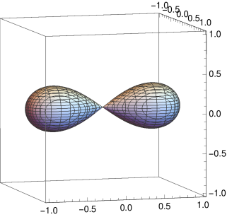
Figure 4.1. The Clifford spectrum of the three scaled Pauli Spin $\Lambda\left(\tfrac{1}{2}\sigma_{x},\sigma_{y},\tfrac{1}{2}\sigma_{z}\right)$ as explained in Example 4.2. The index at a point inside either lobe is $1$. As always, for points on the outside the index is $0$. See the supplemental files Lemniscate.* for the calculations.

Example 4.1.

The first example with Clifford spectrum a surface was due to by Kisil [6], and we repeat that here. The Pauli Spin matrices themselves are the three Hermitian matrices we consider. The following can be computed by hand, but using symbolic algebra is preferred. We find

$$\text{char}\left(\sigma_{x},\sigma_{y},\sigma_{z}\right)=(x^{2}+y^{2}+z^{2}-1)(x^{2}+y^{2}+z^{2}+3)$$

and that here the Clifford spectrum is the unit sphere.

Example 4.2.

A slight modification of the previous example leads to the Clifford spectrum being a surface but not a manifold. We simply rescale some of the Pauli Spin matrices and consider $\tfrac{1}{2}\sigma_{x}$, $\sigma_{y}$ and $\tfrac{1}{2}\sigma_{z}$. The characteristic polynomial is now

$$\textnormal{char}\left(\tfrac{1}{2}\sigma_{x},\sigma_{y},\tfrac{1}{2}\sigma_{z}\right)=(x^{2}+y^{2}+z^{2})^{2}+2z^{2}+2x^{2}-y^{2}$$

Since $(x^{2}+y^{2})^{2}+2x^{2}-y^{2}=0$ describes a lemniscate of Bernoulli, the surface here is a rotated lemniscate as illustrated by Figure 4.1.

Mathematica and other computer algebra programs can produce accurate and compelling pictures of the Clifford spectrum in many examples, but there are limitations. Some rather simple examples can lead to the plot being incomplete, as we will demonstrate. We are asking a computer to verify that a certain set is infinite, which is too big of a request. Two methods are available to verify the results of some examples. The first is to factor the characteristic polynomial and identify the zero-sets of the factors, which might be impossible. The second is to employ the information we get from the $K$-theory indices associated to almost commuting matrices [9]. These generally must be zero when the Clifford spectrum is a finite set, so calculating a single index can tell us that that a certain spectrum is an infinite set.

The index we start with is the most basic of those introduced in [9]. It is defined in terms of the signature. For an invertible Hermitian matrix, the signature is the the number of positive eigenvalues, minus the number of negative eigenvalues, of that matrix.

Definition 4.3.

The index at $\boldsymbol{\lambda}$ for an ordered triple of non-commuting Hermitian matrices $X_{1},X_{2},X_{3}$ is defined only when $\boldsymbol{\lambda}$ is not in $\Lambda(X_{1},X_{2},X_{3}),$ and is given by,

$$\textnormal{Ind}_{\boldsymbol{\lambda}}(X_{1},X_{2},X_{3})=\dfrac{1}{2}\textnormal{Sig}\left(L_{\boldsymbol{\lambda}}(X_{1},X_{2},X_{3})\right).$$

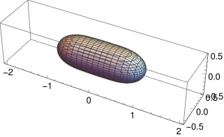
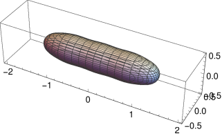
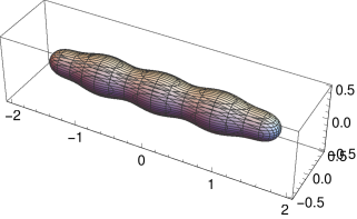
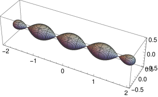
Figure 4.2. The Clifford spectrum of the matrices from Example 4.4. The values of $t$, starting at the top-left, $\tfrac{1}{2}$, $t=\tfrac{2}{3}\dots$, $t=\tfrac{5}{6}$, $t=1$. See supplemental files FSscaled5Croped.* as well as the video file C5scale_cmprsd.avi that shows the Clifford spectrum at many more points on the path.

The index at the origin it $1$ for the Pauli spin matrices, as in Example 4.1. Inside either lobe of the lemniscate example this index is also $1$. These facts can be calculated by hand, or one can see the supplemental files PauliSpinTwoSphere.* and Lemniscate.* for the calculations.

Consider a path $\boldsymbol{\lambda}_{t}$ in $\mathbb{R}^{3}$ with fixed $X_{1},X_{2},X_{3}$, and assume that

$$\textnormal{Ind}_{\boldsymbol{\lambda}_{t_{0}}}(X_{1},X_{2},X_{3})\neq\textnormal{Ind}_{\boldsymbol{\lambda}_{t_{1}}}(X_{1},X_{2},X_{3}).$$

Since the localizer is Hermitian, the only for this change to occur is if the localizer becomes singular at some intermediate $t$. Thus any path between two points with differing index must cross the Clifford spectrum.

It is easy to prove that if $\boldsymbol{\lambda}$ is larger than $\|L_{\mathbf{0}}{(X_{1},X_{2},X_{3})}\|$ then the index at $\boldsymbol{\lambda}$ equals zero. Thus proving that the index to be nonzero at a single point shown that the Clifford spectrum separates that point from infinity. This proves that in that instance the Clifford spectrum is not a finite set.

Already with $2$-by-$2$ matrices, we start to see interesting topology emerge. Moving up to $5$-by-$5$ and $6$-by-$6$ and taking paths of Hermitian matrices, we see the suggestions of interesting patterns. Here we present some of what we found. We encourage the reader to use our Mathematica supplemental files, or the SageMath code listing in [13], as a basis to explore more examples.

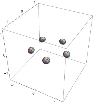
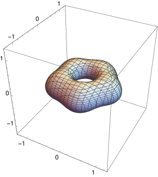
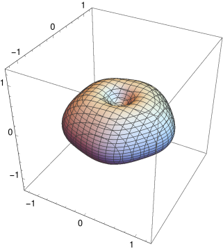
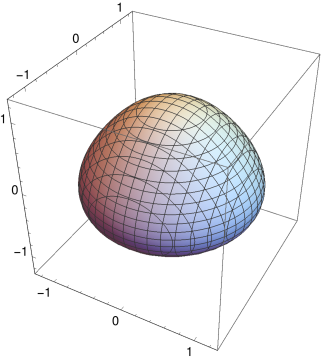
Figure 4.3. The Clifford spectrum of of Example 4.5 for $R=0.9$ and from top-left, $r=\tfrac{4}{10}$, $r=\tfrac{6}{10}$, $r=\tfrac{7}{10},$ and $r=1$. The Clfford spectrum for more values of $r$ can be seen in the supplementary file F5scale_cmprsd.*, and the code to create these plots is in the supplementary file FSscaled5Croped.avi.

Example 4.4.

Berenstein, Dzienkowski, and Lashof-Regas [1, 2] looked at the matrices generating a fuzzy sphere. We consider here similar matrices,

$$A=\begin{bmatrix}2&0&0&0&0\\ 0&1&0&0&0\\ 0&0&0&0&0\\ 0&0&0&-1&0\\ 0&0&0&0&-2\end{bmatrix},\ B=\begin{bmatrix}0&\tfrac{1}{4}&0&0&0\\ \tfrac{1}{4}&0&\tfrac{1}{4}&0&0\\ 0&\tfrac{1}{4}&0&\tfrac{1}{4}&0\\ 0&0&\tfrac{1}{4}&0&\tfrac{1}{4}\\ 0&0&0&\tfrac{1}{4}&0\end{bmatrix},\ C=\begin{bmatrix}0&-\tfrac{i}{4}&0&0&0\\ \tfrac{i}{4}&0&-\tfrac{i}{4}&0&0\\ 0&\tfrac{i}{4}&0&-\tfrac{i}{4}&0\\ 0&0&\tfrac{i}{4}&0&-\tfrac{i}{4}\\ 0&0&0&\tfrac{i}{4}&0\end{bmatrix}.$$

By rescaling one of these matrices, we were able to see a higher iteration of the lemniscate surface. Specifically we looked along the path $(tA,B,C).$ We show in Figure 4.2 the Clifford spectrum at some points along this path.

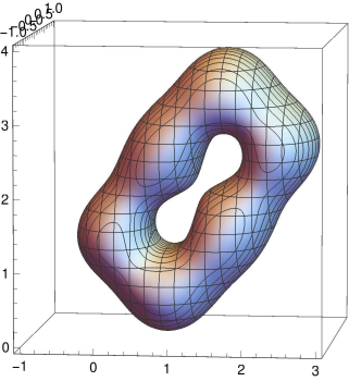
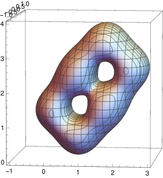
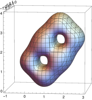
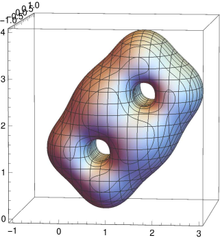
Figure 4.4. A two-holed torus, and a deformation of that, arising as the Clifford spectrum of the three matrices in Example 4.6. Starting at the top-right, the values of $r$ used are $r=\tfrac{1}{2}$, $r=\tfrac{2}{3}$, $r=\tfrac{5}{6}$, $r=1$. The Clfford spectrum for more values of $r$ can be seen in the supplementary file lowering_genus_cmprsd.avi, and the code to create these plots is in the supplementary files two_holes.*. The index calculation in shown in supplementary files two_holes_6_index.*.

Example 4.5.

This example is similar to one in [2], illustrating a transition in the Clifford spectrum between a torus and a sphere. As we want a torus, it is not surprising we start with the clock $V=V_{n}$ and shift $U=U_{n}$ unitaries from (3.4) and (3.5). In Section 5 we will consider Clifford spectrum of four Hermitian matrices and see again a torus. Here we want three matrices, so inspired by the usual parameterization of a torus embedded in three-space we define

$$\begin{aligned} A&=\tfrac{1}{2}\left(R+\tfrac{r}{2}U^{*}+\tfrac{r}{2}U\right)V^{*}+\tfrac{1}{2}V\left(R+\tfrac{r}{2}U^{*}+\tfrac{r}{2}U\right)\\ B&=\tfrac{i}{2}\left(R+\tfrac{r}{2}U^{*}+\tfrac{r}{2}U\right)V^{*}-\tfrac{i}{2}V\left(R+\tfrac{r}{2}U^{*}+\tfrac{r}{2}U\right)\\ C&=\tfrac{ri}{2}U^{*}-\tfrac{ri}{2}U.\end{aligned}$$

We compute this specifically with $n=5$, outer radius $R=0.9$ and variable inner radius $r$. For four values of $r$ lead to the Clifford spectrum shown in Figure 4.3.

Example 4.6.

Taking a hint from [13] we consider

$$\begin{aligned} X&=\begin{bmatrix}\frac{4}{5}&\frac{1}{2}&\frac{1}{2}\\ \frac{1}{2}&0&&\frac{1}{2}\\ \frac{1}{2}&&\frac{8}{5}&\frac{r}{2}&\frac{1}{2}\\ &\frac{1}{2}&\frac{r}{2}&\frac{4}{5}&&\frac{1}{2}\\ &&\frac{1}{2}&&\frac{12}{5}&\frac{1}{2}\\ &&&\frac{1}{2}&\frac{1}{2}&\frac{8}{5}\end{bmatrix},\quad Y=\begin{bmatrix}0&-\frac{i}{2}&-\frac{i}{2}\\ \frac{i}{2}&0&&-\frac{i}{2}\\ \frac{i}{2}&&0&-\frac{ir}{2}&-\frac{i}{2}\\ &\frac{i}{2}&\frac{ir}{2}&0&&-\frac{i}{2}\\ &&\frac{i}{2}&&0&-\frac{i}{2}\\ &&&\frac{i}{2}&\frac{i}{2}&0\end{bmatrix}\\ Z&=\begin{bmatrix}0\\ &\frac{13}{10}\\ &&\frac{13}{10}\\ &&&\frac{13}{5}\\ &&&&\frac{13}{5}\\ &&&&&\frac{39}{10}\end{bmatrix}\end{aligned}$$

which, for $r=1$ is the smallest triples of matrices Sykora found that had Clifford spectrum a two-holed torus. We computed numerically that index is for $r=1$ at $(2,0,0.25)$ inside the two-holed torus to confirm we actually have a surface and not a cloud of points. The plots of the Clifford spectrum for several values of $r$ are shown in Figure 4.4 .

5. Four Hermitian matrices

We need to make a choice of $\gamma_{1},\dots,\gamma_{4}$, and warn the reader that these are related to but not equal to the Dirac matrices. The Dirac matrices square sometimes to $1$ and sometimes to $-1$. Here we need the relations (1.1) which dictate that the matrices are all Hermitian and square to $1$. Moreover, we have no use for a $\gamma_{0}$ as we just want a linearly independent set. We use the Pauli spin matrices for convenience, but there is no connection here with the spin of a particle.

Our choice here is as follows.

(5.1) $$\gamma_{1} =\sigma_{x}\otimes(-\sigma_{y})=\begin{bmatrix}0&0&0&i\\ 0&0&i&0\\ 0&-i&0&0\\ -i&0&0&0\\ \end{bmatrix},\quad\gamma_{2}=\sigma_{y}\otimes(-\sigma_{y})=\begin{bmatrix}0&0&0&-1\\ 0&0&1&0\\ 0&1&0&0\\ -1&0&0&0\\ \end{bmatrix}$$

$$\gamma_{3} =\sigma_{z}\otimes(-\sigma_{y})=\begin{bmatrix}0&0&i&0\\ 0&0&0&-i\\ -i&0&0&0\\ 0&i&0&0\\ \end{bmatrix},\quad\gamma_{4}=I_{2}\otimes(\sigma_{x})=\begin{bmatrix}0&0&1&0\\ 0&0&0&1\\ 1&0&0&0\\ 0&1&0&0\\ \end{bmatrix}$$

The advantage these have is each $\gamma_{j}$ is block off-diagonal. We can thus define the reduced localizer

(5.2) $$\widetilde{L}_{\boldsymbol{\lambda}}(X_{1},X_{2},X_{3},X_{4})=\sum_{k=1}^{3}(X_{k}-\lambda_{k})\otimes\widetilde{\gamma}_{k}$$

in terms of the upper-right blocks of the $\gamma_{j}$. Thus

$$\widetilde{\gamma}_{1}=i\sigma_{x},\ \widetilde{\gamma}_{2}=i\sigma_{y},\ \widetilde{\gamma}_{3}=i\sigma_{z},\ \widetilde{\gamma}_{4}=I_{2}.$$

With this notation, the localizer becomes

$$\widetilde{L}_{\boldsymbol{\lambda}}(X_{1},X_{2},X_{3},X_{4})=\begin{bmatrix}0&\widetilde{L}_{\boldsymbol{\lambda}}(X_{1},X_{2},X_{3},X_{4})\\ (\widetilde{L}_{\boldsymbol{\lambda}}(X_{1},X_{2},X_{3},X_{4}))^{*}&0\end{bmatrix}$$

and the characteristic polynomial can be computed via the formula

$$\left|\textnormal{char}_{\boldsymbol{\lambda}}(X_{1},X_{2},X_{3},X_{4})\right|=\left|\det\left(\widetilde{L}_{\boldsymbol{\lambda}}(X_{1},X_{2},X_{3},X_{4})\right)\right|^{2}$$

Thus we have what we call the reduced characteristic polynomial

$$\det\left(\widetilde{L}_{\boldsymbol{\lambda}}(X_{1},X_{2},X_{3},X_{4})\right)$$

and we can compute the Clifford spectrum by setting that to zero. In computer calculations, especially, we use $(w,x,y,z)$ in place of $(\lambda_{1},\lambda_{2},\lambda_{3},\lambda_{4})$.

We have a three examples, with Clifford spectrum zero-dimensional, two-dimensional, and three-dimensional. The case of two-dimensional Clifford spectrum in four-space is the most difficult, as such a spectrum will not separate a point from infinity. This means there will be no possible $K$-theory argument, and we are stuck with examining a complicated characteristic polynomial. The significance of the reduced characteristic polynomial is that cuts down by half the degree of the polynomial we must study.

To get a torus in four space, we are able to use the Hermitian and anti-Hermitian parts of the clock and shift unitaries. These are all symmetric matices (equal under the transpose $(\mbox{--})^{\mathrm{T}}$) except the imaginary part of the shift, which is anti-symmetric. The following lemma helps simplify things with that symmetry.

Lemma 5.1.

Suppose that $X_{1},X_{2},X_{3},X_{4}$ are Hermitian matrices, that $X_{1}$, $X_{3}$ and $X_{4}$ are symmetric and $X_{2}$ is anti-symmetric. Then

$$\det\left(\widetilde{L}_{(\lambda_{1},-\lambda_{2},\lambda_{3},\lambda_{4})}(X_{1},X_{2},X_{3},X_{4})\right)=\det\left(\widetilde{L}_{(\lambda_{1},\lambda_{2},\lambda_{3},\lambda_{4})}(X_{1},X_{2},X_{3},X_{4})\right).$$

Proof.

We observe that

$$\widetilde{\gamma}_{k}^{\mathrm{T}}=\begin{cases}\widetilde{\gamma}_{k}&\mbox{if }k\neq 2\\ -\widetilde{\gamma}_{k}&\mbox{if }k=2\end{cases}$$

and similarly we have the assumption

$$X_{k}^{\mathrm{T}}=\begin{cases}X_{k}&\mbox{if }k\neq 2\\ -X_{k}&\mbox{if }k=2.\end{cases}$$

so we get that every term $X_{k}\otimes\widetilde{\gamma}_{k}$ is symmetric. On the other hand, every term $\lambda_{k}I_{n}\otimes\widetilde{\gamma}_{k}$ is symmetric except for $k=2$, where that term is anti-symmetric. Let $\epsilon_{j}=1$ except for $\epsilon_{2}=-1$. Then we have

$$\left(\sum_{k=1}^{3}(X_{k}-\lambda_{k})\otimes\widetilde{\gamma}_{k}\right)^{\mathrm{T}} =\left(\sum_{k=1}^{3}X_{k}\otimes\widetilde{\gamma}_{k}\right)^{\mathrm{T}}+\left(\sum_{k=1}^{3}\lambda_{k}I_{k}\otimes\widetilde{\gamma}_{k}\right)^{\mathrm{T}}$$

$$=\sum_{k=1}^{3}(X_{k}-\lambda_{k})\otimes\widetilde{\gamma}_{k}+\sum_{k=1}^{3}\epsilon_{j}\lambda_{k}I_{k}\otimes\widetilde{\gamma}_{k}$$

$$=\sum_{k=1}^{3}(X_{k}-\epsilon_{j}\lambda_{k})\otimes\widetilde{\gamma}_{k}$$

Since the transpose does not effect the determinant, the result follows. ∎

$n$	Imaginary part of reduced characteristic polynomial
$3$	$\left(w^{2}+x^{2}-y^{2}-z^{2}\right)\left(\frac{3}{2}\sqrt{3}\right)$
$4$	$\left(w^{2}+x^{2}-y^{2}-z^{2}\right)\left(4w^{2}+4x^{2}+4y^{2}+4z^{2}+8\right)$
$5$	$\left(w^{2}+x^{2}-y^{2}-z^{2}\right)\left(\frac{5}{2}\sqrt{\frac{1}{2}\left(65+29\sqrt{5}\right)}+[\cdots]+\frac{5}{2}\sqrt{\frac{1}{2}\left(5+\sqrt{5}\right)}z^{4}\right)$
$6$	$\left(w^{2}+x^{2}-y^{2}-z^{2}\right)\left(\frac{3}{2}\sqrt{3}\left(w^{2}+x^{2}+y^{2}+z^{2}+2\right)\left([\cdots]\right)\right)$

Table 1. The imaginary parts of the reduced characteristic polynomials used in the proof of Theorem 5.2. For the full polynomials and how they are calculated, see the supplementary files torus_4_n*.*, in particular the variable impoly.

$n$	Effective real part of reduced characteristic polynomial
$3$	$(-2\cos(3\phi)-2\cos(3\theta))r^{3}+8r^{6}+12r^{4}+3r^{2}-1$
$4$	$r^{4}(-2\cos(4\phi)-2\cos(4\theta)+20)+16r^{8}+32r^{6}-4$
$5$	$32r^{10}+80r^{8}+\left(65+5\sqrt{5}\right)r^{6}+(-2\cos(5\phi)-2\cos(5\theta))r^{5}+[\cdots]$
$6$	$64r^{12}+192r^{10}+240r^{8}+(-2\cos(6\phi)-2\cos(6\theta)+148)r^{6}+9r^{4}-54r^{2}-27$

Table 2. Real parts of the reduced characteristic polynomials used in the proof of Theorem 5.2. See the supplementary files torus_4_n*.*, in particular the variable altpoly.

$n$	Derivatives in $r$ of the Effective real parts
$3$	$(-6\cos(3\phi)-6\cos(3\theta))r^{2}+48r^{5}+48r^{3}+6r$
$4$	$r^{3}(-8\cos(4\phi)-8\cos(4\theta)+80)+128r^{7}+192r^{5}$
$5$	$320r^{9}+640r^{7}+\left(390+30\sqrt{5}\right)r^{5}+(-10\cos(5\phi)-10\cos(5\theta))r^{4}+[\cdots]$
$6$	$768r^{11}+1920r^{9}+1920r^{7}+(-12\cos(6\phi)-12\cos(6\theta)+888)r^{5}+36r^{3}-108r$

Table 3. Derivatives in $r$ of the function in Table 2.

Theorem 5.2.

Suppose $n$ equals $3$, $4$, $5$ or $6$, and define

$$X_{1} =\tfrac{1}{2}U_{n}^{*}+\tfrac{1}{2}U_{n},\quad X_{2} =\tfrac{i}{2}U_{n}^{*}-\tfrac{i}{2}U_{n}$$

$$X_{3} =\tfrac{1}{2}V_{n}^{*}+\tfrac{1}{2}V_{n},\quad X_{4} =\tfrac{i}{2}V_{n}^{*}-\tfrac{i}{2}V_{n}$$

where $U_{n}$ and $V_{n}$ are the clock and shift unitaries as in (3.4) and (3.5). Then the Clifford spectrum of $(X_{1},X_{2},X_{3},X_{4})$ is homeomorphic to a two-torus.

Proof.

We would like to solve for where the reduced localizer is zero,

(5.3) $$\det\left(\widetilde{L}_{\boldsymbol{\lambda}}(X_{1},X_{2},X_{3},X_{4})\right)=0.$$

We will do that in the following way. First, we will find the condition for the imaginary part of the localizer to be zero. Then, after setting its imaginary part to zero, we will show that the real part has both positive and negative values, which implies that it crosses zero at some point. Therefore, at the latter point both real and imaginary parts are zero, which means the whole thing is zero.

We let used computer algebra to calculate and simplify the reduced characteristic polynomial, with results as shown in Table 1. In all cases, the condition $\Im\det\widetilde{L}_{(w,x,y,z)}=0$ becomes

(5.4) $$w^{2}+x^{2}=y^{2}+z^{2}.$$

We now apply Lemma 5.1 and deduce we have $(w,x,y,z)$ in the Clifford spectrum if, and only if, $(w,-x,y,z)$ is the Clifford spectrum. Thus we are justified in assuming $x\geq 0$. With this assumption, the condition $\Im\det\widetilde{L}_{(w,x,y,z)}=0$ becomes

$$x=\sqrt{-w^{2}+y^{2}+z^{2}}.$$

This means we can eliminate $x$ in the polynomial $\Re\det\widetilde{L}_{(w,x,y,z)}$ via the substitution

$$x\mapsto\sqrt{-w^{2}+y^{2}+z^{2}}.$$

With this substitution, we get a somewhat more reasonable polynomial. In the case of $n=3$ it is

$$\begin{gathered}-8w^{3}+3z^{2}\left(2w+8y\left(y^{3}+y\right)+2y+1\right)\\ +6wy^{2}+8y^{6}+12y^{4}-2y^{3}\\ +12\left(2y^{2}+1\right)z^{4}+3y^{2}+8z^{6}-1\end{gathered}$$

and for $n=4,5,6$ this polynomial has too many terms to easily display. It but can be seen as realpoly in the supplementary files torus_4_n*.*.

Inspired by (5.4) we switch to polar coordinates in the first two and also the last two variables, as we know the radius will be the same. That is, we make the substitution

(5.5) $$w =r\cos\theta,\quad x =r\sin\theta$$

$$y =r\cos\phi,\quad z =r\sin\phi$$

and find the computer does a much better job simplifying. The Clifford spectrum will be the zero set of the functions shown in Table 2, interpreted via (5.5). The function in the $n=5$ case was too long for the table, but can be seen as altpoly in the supplementary files torus_4_n5.*.

Now we finish the proof for the case $n=4$, which is the easiest case. Let’s denote the relevant function from Table 2 by $f(r,\theta,\phi)$, so

$$f(r,\theta,\phi)=-4+32r^{6}+16r^{8}+(20-2\cos(4\phi)-2\cos(4\theta))r^{4}$$

and its $r$ derivative is

$$\frac{\partial f}{\partial r}=192r^{5}+128r^{7}+(80-8\cos(4\phi)-8\cos(4\theta))r^{3}.$$

Since sine and cosine are bounded by $\pm 1$ we see that, for any angles $\phi$ and $\theta$, $\frac{\partial f}{\partial r}>0$ for all $r>0$ and so $f(r,\theta,\phi)$ is increasing for $r\geq 0$. By observing that

$$f(\theta,\phi,0)=-4$$

and

$$\lim_{r\rightarrow\infty}f(\theta,\phi,r)=\infty$$

we know that, for any fixed $(\theta,\phi)$, there exist at least one value of $r$ for which $f(\theta,\phi,r)=0$, and the fact that $\partial f/\partial r>0$ implies that this value of $r$ is unique. Call this value $\rho(\theta,\phi)$, so

$$f(\theta,\phi,\rho(\theta,\phi))=0$$

Thus, the surface we are looking for is precisely the surface $r=\rho(\theta,\phi)$, which is indeed topologically equivalent to a torus since $\rho(\theta,\phi)$ must vary continuously in $\theta$ and $\phi$ since the roots of a polynomial vary continuous with respect to the coefficients [5]. The resulting surface in illustrated in Figure 5.1.

Now we look at the case $n=3$. The relevant function from Table 2 is

$$f(r,\theta,\phi)=(-2\cos(3\phi)-2\cos(3\theta))r^{3}+8r^{6}+12r^{4}+3r^{2}-1$$

with derivative in $r$ being

$$\frac{\partial f}{\partial r}=(-6\cos(3\phi)-6\cos(3\theta))r^{2}+48r^{5}+48r^{3}+6r$$

For $0<r\leq\tfrac{1}{2}$ we have the estimate

$$\frac{\partial f}{\partial r} >(-6\cos(3\phi)-6\cos(3\theta))r^{2}+6r$$

$$\geq(-12r+6)r\geq 0$$

and for $\tfrac{1}{2}\leq r\leq 1$ we have the estimate

$$\frac{\partial f}{\partial r} >(-6\cos(3\phi)-6\cos(3\theta))r^{2}+48r^{3}$$

$$\geq(-12+48r)r^{2}\geq 0$$

so again the derivative is positive except at zero it is zero. The rest of the proof follows as in the case $n=4$. The resulting surface in illustrated in Figure 5.2.

For the case $n=5$ one can prove that for $0\leq r\leq\tfrac{3}{5}$,

$$f(r,\theta,\phi)\leq-2$$

and, for $\tfrac{3}{5}\leq r\leq 1$,

$$\frac{\partial f}{\partial r}\geq 33$$

so again we see that for each pair of angles there is only one radius to make this function zero. The work to create these two estimates is shown in the supplementary files torus_4_n5.*.

For the case $n=6$ one can prove that for $0\leq r\leq\tfrac{3}{5}$,

$$f(r,\theta,\phi)\leq-20$$

and, for $\tfrac{3}{5}\leq r\leq 1$,

$$\frac{\partial f}{\partial r}\geq 42$$

so again we see that for each pair of angles there is only one radius to make this function zero. The work to create these two estimates is shown in the supplementary files torus_4_n6.*.

∎

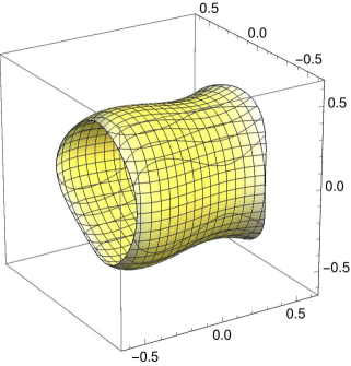
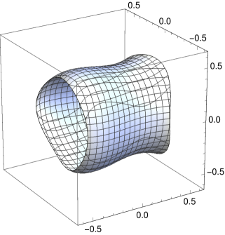
Figure 5.1. The Clifford spectrum as a surface in four space. The top and bottom represent half the surface, with color indicating the value in the fourth dimension — white indicates zero, shades of yellow indicate positive values, and shades of blue negative values. This is for the for Hermitian matrices extracted from the clock and shift matrices, with $n=3$.

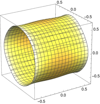
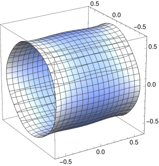
Figure 5.2. The Clifford spectrum as a surface in four space, for the Hermitian matrices extracted from the clock and shift matrices, with $n=4$.

Example 5.3.

In example 4.1 we saw that the Clifford spectrum of the gamma matrices lead to a sphere. Taking the Clifford spectrum of the four gamma matrices (5.1) gives a somewhat different answer. In the supplementary file GammaMatrices_4B.* is are the symbolic calculations that for these four matrices the reduced characteristic polynomial is

$$\left(w^{2}+x^{2}+y^{2}+z^{2}\right)^{3}\left(w^{2}+x^{2}+y^{2}+z^{2}+8\right)$$

and so the Clifford spectrum is a single point.

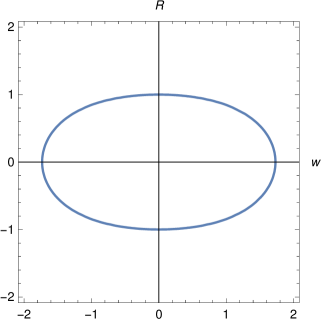
Figure 5.3. The Clifford spectrum in Example 5.4 is this curve rotated in the two additional dimensions.

Example 5.4.

Now we look at a rescaling of the four gamma matrices (5.1),

$$X_{1}=2\gamma_{1},\quad X_{2}=\gamma_{2},\quad X_{3}=\gamma_{3},\quad X_{4}=\gamma_{4}.$$

and find, in supplementary file GammaMatrices_4A.*, that the reduced characteristic polynomial is

$$(9+6R^{2}+R^{4}-6w^{2}+2R^{2}w^{2}+w^{4})(-15+14R^{2}+R^{4}+2w^{2}+2R^{2}w^{2}+w^{4})$$

where $R=\sqrt{x^{2}+y^{2}+z^{2}}$. For this example, the Clifford spectrum is homeomorphic to the three-sphere. See Figure 5.4.

6. Symmetry classes and $K$-theory charges

6.1. Where the index and plotting fail

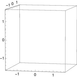
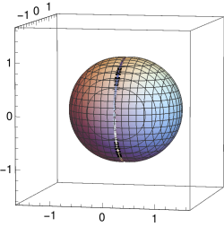
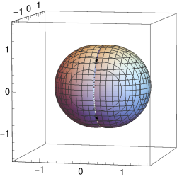
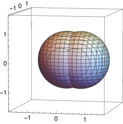
Figure 6.1. An example where we cannot trust the plot via the characteristic polynomial. This is using matrices as in Example 6.1, with $r=0$ at the top left, increasing by $1/6$ and ending at the bottom right with $r=1/2$. The code to create these graphics are in the in the supplementary files ClassAIIsphere.*.

We have the index to give us critical information about the surfaces we have plotted. Sometimes the Clifford spectrum is a surface but the index is zero everywhere it is defined. Moreover, in those situations the computer plotting can fail.

Example 6.1.

The three matrices we consider are as follows:

(6.1) $$X=\begin{bmatrix}0&1&0&0\\ 1&0&0&0\\ 0&0&0&1\\ 0&0&1&0\end{bmatrix},\,Y=\begin{bmatrix}0&-i&0&0\\ i&0&0&0\\ 0&0&0&i\\ 0&0&-i&0\end{bmatrix},\,Z=\begin{bmatrix}1&0&0&0\\ 0&-1&0&0\\ 0&0&1&0\\ 0&0&0&-1\end{bmatrix}.$$

Since the characteristic polynomial respects direct sums, it is easy to see from Example 4.1 that the characteristic polynomial is

$$\text{char}\left(\sigma_{x},\sigma_{y},\sigma_{z}\right)=(x^{2}+y^{2}+z^{2}-1)^{2}(x^{2}+y^{2}+z^{2}+3)^{2}$$

so the Clifford spectrum is the unit sphere. Also, by looking at the direct sum structure, one can check that the index zero at the origin. Thus the index is zero everywhere it is defined. Figure 6.1 looks at the plot Mathematica makes using the characteristic polynomial for

(6.2) $$X_{r}=\begin{bmatrix}0&1&0&0\\ 1&0&0&0\\ 0&0&r&1\\ 0&0&1&r\end{bmatrix},\,Y_{r}=\begin{bmatrix}0&-i&0&0\\ i&0&0&0\\ 0&0&0&i\\ 0&0&-i&0\end{bmatrix},\,Z_{r}=\begin{bmatrix}1&0&0&0\\ 0&-1&0&0\\ 0&0&1&0\\ 0&0&0&-1\end{bmatrix}$$

for various small values of $r$, and also at zero. At zero the output is the null plot, which is wrong.

6.2. A refined index in the case of self-dual symmetry

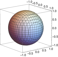
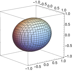
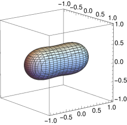
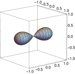
Figure 6.2. The self dual matrices from Example 6.3, plotted using the archetypal polynomial. This is using matrices of Equation 6.3, with $s=0$ at the top left, increasing by $1/6$ and ending at the bottom right with $s=1/2$. Plots made using the supplemntary file ClassAIIspherePfaff.nb.

.

In the case of the matrices in Equation 6.1, the matrices had an extra symmetry that went unused. They are all self-dual, a mathematical interpretation of having fermionic time reversal symmetry.

Recall that the dual operation is defined as,

$$X^{\#}={\begin{bmatrix}A&B\\ C&D\end{bmatrix}}^{\#}=\begin{bmatrix}D^{T}&-B^{T}\\ -C^{T}&A^{T}\end{bmatrix},$$

where $A,B,C,$ and $D$ are square complex matrices. When a matrix $X$ is self-dual and Hermitian, we have both, $X^{\#}=X$ and $X^{*}=X.$

If we have three matrices that are Hermitian and self-dual, we find that the localizer has an extra symmetry. In this case, there is a matrix $Q$ that conjugates the spectral localizer nicely, given by

$$Q=\begin{bmatrix}I_{2n}&-iZ_{2n}\\ iZ_{2n}&I_{2n}\end{bmatrix}$$

where

$$Z_{2n}=\begin{bmatrix}0&I_{n}\\ -I_{n}&0\end{bmatrix}.$$

Conjugating the spectral localizer, by the unitary matrix $\tfrac{1}{\sqrt{2}}Q$ we keep the determinant unchanged. That is,

$$\Big{(}\tfrac{1}{\sqrt{2}}Q\Big{)}^{*}L_{\boldsymbol{\lambda}}(A,B,C)\Big{(}\tfrac{1}{\sqrt{2}}Q\Big{)}=\tfrac{1}{2}Q^{*}L_{\boldsymbol{\lambda}}(A,B,C)Q$$

and

$$\text{det}\left(\tfrac{1}{2}Q^{*}L_{\boldsymbol{\lambda}}(A,B,C)Q\right)=\text{det}(L_{\boldsymbol{\lambda}}(A,B,C))=\text{char}_{\boldsymbol{\lambda}}(A,B,C).$$

Using Lemma $8.1$ of Factorization of Matrices of Quaternions [8] we confirm that the conjugation produces a skew-symmetric representation of the localizer and therefore,

$$\left(\tfrac{1}{2}Q^{*}L_{\boldsymbol{\lambda}}(A,B,C)Q\right)^{\mathrm{T}}=-\tfrac{1}{2}Q^{*}L_{\boldsymbol{\lambda}}(A,B,C)Q$$

We can now use the pfaffian instead of the determinant to detect where the localizer is singular.

Definition 6.2.

The archetypal polynomial of a self-dual Hermitian triple $(X,Y,Z)$ is defined as

$$\textnormal{arch}_{\boldsymbol{\lambda}}(X,Y,Z)=\textnormal{Pf}\left(\tfrac{1}{2}Q^{*}L_{\boldsymbol{\lambda}}(X,Y,Z)Q\right).$$

Example 6.3.

We look at a different path that starts with the troublesome matrices of (6.1). For $0\leq s\leq\tfrac{1}{2}$ we define matrices

(6.3) $$X_{s}= \begin{bmatrix}0&1-2s&0&s\\ 1-2s&0&-s&0\\ 0&s&0&1-2s\\ -s&0&1-2s&0\end{bmatrix},\quad Y_{s}=\begin{bmatrix}0&-i&0&0\\ i&0&0&0\\ 0&0&0&i\\ 0&0&-i&0\end{bmatrix},$$

$$Z_{s}= \begin{bmatrix}1-s&0&0&0\\ 0&-1+s&0&0\\ 0&0&1-s&0\\ 0&0&0&-1+s\end{bmatrix}$$

which are self-dual and Hermitian. Here the plotting looks a lot better, shown in Figure 6.2. Also, we can calculate a $\mathbb{Z}_{2}$ invariant, the sign of the archetypal polynomial. Again, this is known to be trivial ($+1$) far from the origin, and so a value of $-1$ of the invariant disallows finite cardinality of the Clifford spectrum.

6.3. An index for even and odd matrices

Moving up a dimension, consider

(6.4) $$X =\begin{bmatrix}0&2&0&0\\ 2&0&0&0\\ 0&0&0&-2\\ 0&0&-2&0\end{bmatrix},\quad Y=\begin{bmatrix}0&-i&0&0\\ i&0&0&0\\ 0&0&0&-i\\ 0&0&-i&0\end{bmatrix},$$

$$Z =\begin{bmatrix}1&0&0&0\\ 0&-1&0&0\\ 0&0&-1&0\\ 0&0&0&1\end{bmatrix},\quad H=\begin{bmatrix}0&0&1&0\\ 0&0&0&1\\ 1&0&0&0\\ 0&1&0&0\end{bmatrix}.$$

The characteristic polynomial of these four matrices, computed by the code in the supplementary file Even_odd_4CMathematica.nb, is

$$\left(R^{4}+2R^{2}w^{2}+6R^{2}+w^{4}-6w^{2}+9\right)\left(R^{4}+2R^{2}w^{2}+14R^{2}+w^{4}+2w^{2}-15\right)$$

where $R^{2}=x^{2}+y^{2}+z^{2}$. Again we have a surface homeomorphic to a three-sphere.

We introduce a grading via the matrix

$$\Gamma=\begin{bmatrix}1&0&0&0\\ 0&1&0&0\\ 0&0&-1&0\\ 0&0&0&-1\end{bmatrix}$$

so we consider a matrix $M$ even if $M\Gamma=\Gamma M$ and odd if $M\Gamma=-\Gamma M$. In the example under discussion, the first three matrices are even and the last is odd.

With these symmetries, we get an index for points $(w,x,y,z)$ not in the Clifford spectrum and with the restriction that $z=0$. This restriction is needed as translating $H$ will ruin the symmetry $H\Gamma=\Gamma H$. The index is based on the fact that

$$i\widetilde{L}_{\boldsymbol{\lambda}}(X,Y,Z,Y)\left(\Gamma\otimes I_{2}\right)$$

is Hermitian, and the index is

$$\frac{1}{2}\mathrm{Sig}\left(i\widetilde{L}_{\boldsymbol{\lambda}}(X,Y,Z,Y)\left(\Gamma\otimes I_{2}\right)\right).$$

Here we are referring the the reduced localizer of (5.2). This is explained in [10].

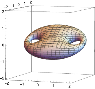
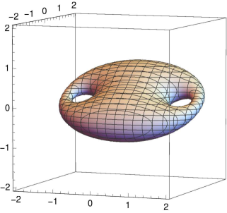
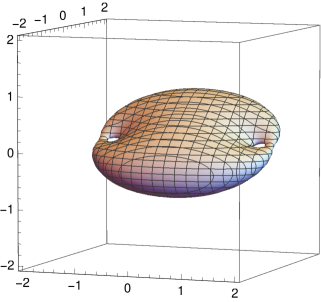
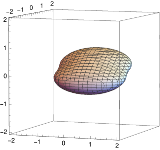
Figure 6.3. This figure shows parts of the Clifford spectrum for the four matrices in (6.5). Shown are slices of the Clifford spectrum in 4-space through the hyperplances $z=0,$ $z=0.2$, $z=0.4$ and $z=0.6$. There is a $\pm z$ symmetry in this example so these images are valid for the corresponding negative values of $z$. This plots we created using the file Even_odd_4A.nb.

For the matrices in (6.4), the index at the origin is $-1$. As always for lambda large compared to the norm of the matrices the index is $0$. Thus the part of the Clifford spectrum that intersects the hyperplane $z=0$ is protected. Small perturbations of the matrices will not change by much the part of the Clifford spectrum intersected with $z=0$.

A little exploration of matrices near these lead to the following. Consider the four matrices

(6.5) $$X =\begin{bmatrix}\tfrac{3}{2}&2&0&0\\ 2&0&0&0\\ 0&0&0&-2\\ 0&0&-2&\tfrac{3}{2}\end{bmatrix},\quad Y=\begin{bmatrix}0&-i&0&0\\ i&0&0&0\\ 0&0&0&-i\\ 0&0&-i&0\end{bmatrix},$$

$$Z =\begin{bmatrix}1&0&0&0\\ 0&-1&0&0\\ 0&0&-1&0\\ 0&0&0&1\end{bmatrix},\quad H=\begin{bmatrix}0&0&1&0\\ 0&0&0&1\\ 1&0&0&0\\ 0&1&0&0\end{bmatrix},$$

so $r=0$ recreates the previous example. Figure 6.3 looks at slices of the Clifford spectrum for this example.

Supplemetary files

The supplementary files are available for download from

math.unm.edu/~loring/CliffordExperiments/

and are all Mathematica files, videos created Mathematica files or a PDF copy of a Mathematica file.

References

- [1] David Berenstein and Eric Dzienkowski, Matrix embeddings on flat and the geometry of membranes, Physical Review D 86 (2012), no. 8, 086001.
- [2] David Berenstein, Eric Dzienkowski, and Robin Lashof-Regas, Spinning the fuzzy sphere, Journal of High Energy Physics 2015 (2015), no. 8, 134.
- [3] Bin Chen and Shao-Ming Fei, Sum uncertainty relations for arbitrary incompatible observables, Scientific reports 5 (2015), 14238.
- [4] Patrick DeBonis, Emergent topology of multivariable spectrum, Bachelor’s thesis, University of New Mexico, 2019.
- [5] Gary Harris and Clyde Martin, Shorter notes: The roots of a polynomial vary continuously as a function of the coefficients, Proceedings of the American Mathematical Society (1987), 390–392.
- [6] Vladimir V. Kisil, Möbius transformations and monogenic functional calculus, Electron. Res. Announc. Amer. Math. Soc. 2 (1996), no. 1, 26–33 (electronic). MR 1405966 (98a:47018)
- [7] Terry Loring and Hermann Schulz-Baldes, The spectral localizer for even index pairings, J. Noncommut. Geom. (2019), to appear, arXiv preprint arXiv:1802.04517.
- [8] Terry A Loring, Factorization of matrices of quaternions, Expositiones Mathematicae 30 (2012), no. 3, 250–267.
- [9] Terry A. Loring, -theory and pseudospectra for topological insulators, Ann. Physics 356 (2015), 383–416. MR 3350651
- [10] Terry A. Loring and Hermann Schulz-Baldes, Finite volume calculation of -theory invariants, New York J. Math. 23 (2017), 1111–1140.
- [11] Susumu Okubo, Real representations of finite Clifford algebras. I. classification, J. math. phys. 32 (1991), no. 7, 1657–1668.
- [12] Lukas Schneiderbauer and Harold C Steinacker, Measuring finite quantum geometries via quasi-coherent states, Journal of Physics A: Mathematical and Theoretical 49 (2016), no. 28, 285301.
- [13] Andreas Sykora, The fuzzy space construction kit, arXiv preprint arXiv:1610.01504 (2016).