Secure connectivity of wireless sensor networks
under key predistribution with on/off channels

Abstract

Security is an important issue in wireless sensor networks (WSNs), which are often deployed in hostile environments. The $q$-composite key predistribution scheme has been recognized as a suitable approach to secure WSNs. Although the $q$-composite scheme has received much attention in the literature, there is still a lack of rigorous analysis for secure WSNs operating under the $q$-composite scheme in consideration of the unreliability of links. One main difficulty lies in analyzing the network topology whose links are not independent. Wireless links can be unreliable in practice due to the presence of physical barriers between sensors or because of harsh environmental conditions severely impairing communications. In this paper, we resolve the difficult challenge and investigate $k$-connectivity in secure WSNs operating under the $q$-composite scheme with unreliable communication links modeled as independent on/off channels, where $k$-connectivity ensures connectivity despite the failure of any $(k-1)$ sensors or links, and connectivity means that any two sensors can find a path in between for secure communication. Specifically, we derive the asymptotically exact probability and a zero-one law for $k$-connectivity. We further use the theoretical results to provide design guidelines for secure WSNs. Experimental results also confirm the validity of our analytical findings.

I Introduction

Since Eschenauer and Gligor [1] introduced the basic key predistribution scheme to secure communication in wireless sensor networks (WSNs), key predistribution schemes have been studied extensively in the literature over the last decade [2, 3, 4, 5, 6, 7]. The idea of key predistribution is that cryptographic keys are assigned before deployment to ensure secure sensor-to-sensor communications.

Among many key predistribution schemes, the $q$-composite scheme proposed by Chan et al. [8] as an extension of the basic Eschenauer–Gligor scheme [1] (the $q$-composite scheme in the case of $q=1$) has received much interest [9, 6, 10, 11, 12]. The $q$-composite key predistribution scheme works as follows. For a WSN with $n$ sensors, prior to deployment, each sensor is independently assigned $K_{n}$ different keys which are selected uniformly at random from a pool $\mathcal{P}_{n}$ of $P_{n}$ distinct keys. After deployment, any two sensors establish a secure link in between if and only if they have at least $q$ key(s) in common and the physical link constraint between them is satisfied. Both $P_{n}$ and $K_{n}$ are both functions of $n$ for generality, with the natural condition $1\leq q<K_{n}<P_{n}$. Examples of physical link constraints include the reliability of the transmission channel and the distance between two sensors close enough for communication. The $q$-composite scheme with $q\geq 2$ outperforms the basic Eschenauer–Gligor scheme with $q=1$ in terms of the strength against small-scale network capture attacks while trading off increased vulnerability in the face of large-scale attacks [8].

In this paper, we investigate $k$-connectivity in secure WSNs employing the $q$-composite key predistribution scheme with general $q$ under the on/off channel model as the physical link constraint comprising independent channels which are either on or off. A network is $k$-connected if it remains connected despite the failure of at most $(k-1)$ nodes, where nodes can fail due to adversarial attacks, battery depletion, or harsh environmental conditions [13]; connectivity ensures that any two nodes can find a path in between [10]. Our results on secure $k$-connectivity include the asymptotically exact probability and also a zero–one law. The zero–one law means that the network is securely $k$-connected with high probability under certain parameter conditions and is not securely $k$-connected with high probability under other parameter conditions, where an event happens “with high probability” if its probability converges to $1$ asymptotically. The zero–one law specifies the critical scaling of the model parameters in terms of secure $k$-connectivity, while the asymptotically exact probability result provides a precise guideline for ensuring secure $k$-connectivity. Obtaining such a precise guideline is particularly crucial in a WSN setting as explained below. To increase the chance of ($k$-)connectivity, it is often required to increase the number of keys kept in each sensor’s memory. However, since sensors have limited memory, it is desirable for practical key distribution schemes to have low memory requirements [1, 14]. Therefore, it is important to obtain the asymptotically exact probability as well as the zero–one law to dimension the $q$-composite scheme.

Our approach to the analysis is to explore the induced random graph models of the WSNs. As will be clear in Section II, the graph modeling a studied WSN is an intersection of two distinct types of random graphs. It is the intertwining [10, 13] of these two graphs that makes our analysis challenging.

We organize the rest of the paper as follows. Section II describes the system model. Afterwards, we detail the analytical results in Section III. We provide experiments in Section IV to confirm our analytical results. Sections V through VIII are devoted to proving the results. Section IX surveys related work. Finally, we conclude the paper in Section X.

II System Model

We elaborate the graph modeling of a WSN with $n$ sensors, which employs the $q$-composite key predistribution scheme and works under the on/off channel model. We use a node set $\mathcal{V}_{n}=\{v_{1},v_{2},\ldots,v_{n}\}$ to represent the $n$ sensors (the terms sensor and node are interchangeable in this paper). For each $v_{i}\in\mathcal{V}_{n}$, the set of its $K_{n}$ different keys is denoted by $S_{i}$, which is uniformly distributed among all $K_{n}$-size subsets of a key pool $\mathcal{P}_{n}$ of $P_{n}$ keys.

The $q$-composite key predistribution scheme is modeled by a uniform $q$-intersection graph [9, 12] denoted by $G_{q}(n,K_{n},P_{n})$, which is defined on the node set $\mathcal{V}_{n}$ such that any two distinct nodes $v_{i}$ and $v_{j}$ sharing at least $q$ key(s) (an event denoted by $\Gamma_{ij}$) have an edge in between. Clearly, event $\Gamma_{ij}$ is given by $\big{[}|S_{i}\hskip 2.0pt{\cap}\hskip 2.0ptS_{j}|\geq q\big{]}$, with $|A|$ denoting the cardinality of a set $A$.

Under the on/off channel model, each node-to-node channel is independently on with probability ${p_{n}}$ and off with probability $(1-{p_{n}})$, where ${p_{n}}$ is a function of $n$ with $0<{p_{n}}\leq 1$. Denoting by ${C}_{ij}$ the event that the channel between distinct nodes $v_{i}$ and $v_{j}$ is on, we have ${\mathbb{P}}\left[{C_{ij}}\right]={p_{n}}$, where $\mathbb{P}[\mathcal{E}]$ denotes the probability that event $\mathcal{E}$ happens, throughout the paper. The on/off channel model is represented by an Erdős-Rényi graph $G(n,{p_{n}})$ [15] defined on the node set $\mathcal{V}_{n}$ such that $v_{i}$ and $v_{j}$ have an edge in between if event $C_{ij}$ occurs.

Finally, we denote by $\mathbb{G}_{n,q}(n,K_{n},P_{n},{p_{n}})$ the underlying graph of the $n$-node WSN operating under the $q$-composite scheme and the on/off channel model. Graph $\mathbb{G}_{n,q}(n,K_{n},P_{n},{p_{n}})$ is defined on the node set $\mathcal{V}_{n}$ such that there exists an edge between nodes $v_{i}$ and $v_{j}$ if and only if events $\Gamma_{ij}$ and $C_{ij}$ happen at the same time. We set event $E_{ij}:=\Gamma_{ij}\cap C_{ij}$. Then the edge set of $\mathbb{G}_{n,q}(n,K_{n},P_{n},{p_{n}})$ is the intersection of the edge sets of $G_{q}(n,K_{n},P_{n})$ and $G(n,{p_{n}})$, so $\mathbb{G}_{n,q}(n,K_{n},P_{n},{p_{n}})$ can be seen as the intersection of $G_{q}(n,K_{n},P_{n})$ and $G(n,{p_{n}})$, i.e.,

$$\mathbb{G}_{n,q}(n,K_{n},P_{n},{p_{n}})=G_{q}(n,K_{n},P_{n})\cap G(n,{p_{n}}),$$ (1)

Throughout the paper, $q$ is an arbitrary positive integer and does not scale with $n$. We define $s(K_{n},P_{n},q)$ as the probability that two different nodes share at least $q$ key(s) and $t(K_{n},P_{n},q,{p_{n}})$ as the probability that two distinct nodes have a secure link in $\mathbb{G}_{n,q}(n,K_{n},P_{n},{p_{n}})$. We often write $s(K_{n},P_{n},q)$ and $t(K_{n},P_{n},q,{p_{n}})$ as $s_{n,q}$ and $t_{n,q}$ respectively for simplicity. Clearly, $s_{n,q}$ and $t_{n,q}$ are the edge probabilities in graphs $G_{q}(n,K_{n},P_{n})$ and $\mathbb{G}_{n,q}(n,K_{n},P_{n},{p_{n}})$, respectively. From $E_{ij}=\Gamma_{ij}\cap C_{ij}$ and the independence of ${C}_{ij}$ and $\Gamma_{ij}$, we obtain

$${t_{n,q}} =\mathbb{P}[E_{ij}]=\mathbb{P}[{C}_{ij}]\cdot\mathbb{P}[\Gamma_{ij}]={p_{n}}\cdot s_{n,q}.$$ (2)

By definition, $s_{n,q}$ is determined through

$$s_{n,q} =\mathbb{P}[\Gamma_{ij}]=\sum_{u=q}^{K_{n}}\mathbb{P}[|S_{i}\cap S_{j}|=u],$$ (3)

where we derive $\mathbb{P}[|S_{i}\cap S_{j}|=u]$ as follows.

Note that $S_{i}$ and $S_{j}$ are independently and uniformly selected from all $K_{n}$-size subsets of a key pool with size $P_{n}$. Under $(|S_{i}\hskip 2.0pt{\cap}\hskip 2.0ptS_{j}|=u)$, after $S_{i}$ is determined, $S_{j}$ is constructed by selecting $u$ keys out of $S_{i}$ and $(K_{n}-u)$ keys out of the key pool $\mathcal{P}_{n}$. Hence, if $P_{n}\geq 2K_{n}$ and $K_{n}\geq q$, we have

$$\mathbb{P}[|S_{i}\cap S_{j}|=u] =\frac{\binom{K_{n}}{u}\binom{P_{n}-K_{n}}{K_{n}-u}}{\binom{P_{n}}{K_{n}}},\quad\text{for }u=1,2,\ldots,K_{n},$$ (4)

which along with (2) and (3) yields

$$t_{n,q}={p_{n}}\cdot\sum_{u=q}^{K_{n}}\frac{\binom{K_{n}}{u}\binom{P_{n}-K_{n}}{K_{n}-u}}{\binom{P_{n}}{K_{n}}}.$$ (5)

Asymptotic expressions of $s_{n,q}$ and $t_{n,q}$ can also be given. If $\frac{{K_{n}}^{2}}{P_{n}}=o(1)$, we obtain from Lemma 2 or [11, Lemma 1] that $s_{n,q}\sim\frac{1}{q!}\big{(}\frac{{K_{n}}^{2}}{P_{n}}\big{)}^{q}$, which with (2) leads to

$$t_{n,q}\sim{p_{n}}\cdot\frac{1}{q!}\bigg{(}\frac{{K_{n}}^{2}}{P_{n}}\bigg{)}^{q}.$$

In the above results, for two positive sequences $f_{n}$ and $g_{n}$, the relation $f_{n}\sim g_{n}$ means $\lim\limits_{n\to\infty}({f_{n}}/{g_{n}})=1$; i.e., $f_{n}$ and $g_{n}$ are asymptotically equivalent.

III The Results

We present and discuss our results in this section. The natural logarithm function is given by $\ln$. All limits are understood with $n\to\infty$. We use the standard asymptotic notation $o(\cdot),O(\cdot),\Omega(\cdot),\omega(\cdot),\Theta(\cdot),\sim$; see [13, Page 2-Footnote 1].

Theorem 1 below presents the asymptotically exact probability and a zero–one law for connectivity in a graph $\mathbb{G}_{n,q}(n,K_{n},P_{n},{p_{n}})$.

Theorem 1.

For a graph $\mathbb{G}_{n,q}(n,K_{n},P_{n},{p_{n}})$, with a sequence $\alpha_{n}$ defined through

$$t_{n,q} =\frac{\ln n+(k-1)\ln\ln n+{\alpha_{n}}}{n},$$ (6)

where $t_{n,q}$ is given by (5), then it holds under $K_{n}=\Omega(n^{\epsilon})$ for a positive constant $\epsilon$, $\frac{{K_{n}}^{2}}{P_{n}}=o\left(\frac{1}{\ln n}\right)$, and $\frac{K_{n}}{P_{n}}=o\left(\frac{1}{n\ln n}\right)$ that

$$\lim_{n\rightarrow\infty}\mathbb{P}\big{[}\mathbb{G}_{n,q}(n,K_{n},P_{n},{p_{n}})\mbox{ is $k$-connected.}\big{]}$$

$$=e^{-\frac{e^{-\lim_{n\to\infty}\alpha_{{}_{n}}}}{(k-1)!}}$$ (7)

$$= e^{-\frac{e^{-\alpha^{*}}}{(k-1)!}}, \lim\limits_{n\to\infty}\alpha_{n}=\alpha^{*}\in(-\infty,\infty)$$ if , (8a)

$$= 1, \lim\limits_{n\to\infty}\alpha_{n}=\infty$$ if , (8b)

$$= 0, \lim\limits_{n\to\infty}\alpha_{n}=-\infty$$ if . (8c)

For $k$-connectivity in $\mathbb{G}_{n,q}(n,K_{n},P_{n},{p_{n}})$, the result (7) of Theorem 1 presents the asymptotically exact probability, while (8c) and (8b) of Theorem 1 together constitute a zero–one law, where a zero–one law means that the probability of a graph having a certain property asymptotically converges to $0$ under some conditions and to $1$ under some other conditions. The result (7) compactly summarizes (8a)–(8c).

Theorem 1 shows that the critical scaling of $t_{n,q}$ for $k$-connectivity in graph $\mathbb{G}_{n,q}(n,K_{n},P_{n},{p_{n}})$ is $\frac{\ln n+(k-1)\ln\ln n}{n}$. The conditions in Theorem 1 are enforced merely for technical reasons, but they are practical and often hold in realistic wireless sensor network applications [8, 16, 1]. More specifically, the condition on $K_{n}$ (i.e., $K_{n}=\Omega(n^{\epsilon})$) is less appealing but is not much a problem because $\epsilon$ can be arbitrarily small. In addition, $\frac{{K_{n}}^{2}}{P_{n}}=o\left(\frac{1}{\ln n}\right)$ and $\frac{K_{n}}{P_{n}}=o\left(\frac{1}{n\ln n}\right)$ hold in practice since the key pool size $P_{n}$ grows at least linearly with $n$ and is expected to be several orders of magnitude larger than the key ring size $K_{n}$ (see [1, Section 2.1] and [10, Section III-B]).

Below, we first provide experimental results before proving Theorem 1 in detail.

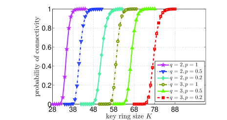
Figure 1: Empirical probability that $\mathbb{G}_{n,q}(n,K,P,{p})$ is connected as a function of $K$ for $q=2,3$ and $p=0.2,0.5,1$ with $n=1,000$ and $P=10,000$. In each case, the empirical probability value is obtained by averaging over $500$ experiments.

IV Experimental Results

We now present experiments to confirm Theorem 1.

In the experiments, we fix the number of nodes at $n=1,000$ and the key pool size at $P=10,000$. We specify the required amount $q$ of key overlap as $q=2,3$, and the probability $p$ of an channel being on as $p=0.2,0.5,1$, while varying the parameter $K$ from $28$ to $88$. For each parameter pair $(q,p,K)$, we generate $500$ independent samples of the graph $\mathbb{G}_{n,q}(n,K,P,{p})$ and count the number of times (out of a possible $500$) that the obtained graphs are connected. Dividing the counts by $500$, we obtain the empirical probabilities for connectivity.

In Figure 1, we depict the resulting empirical probability of connectivity in $\mathbb{G}_{n,q}(n,K,P,{p})$ versus $K$. From Figure 1, the threshold behavior of the probability of connectivity is evident from the plots. Based on (5) and (6), we also compute the minimum integer value of $K^{*}$ that satisfies

$$t(K^{*},P,q,{p})={p}\cdot\sum_{u=q}^{K^{*}}\frac{\binom{K^{*}}{u}\binom{P-K^{*}}{K^{*}-u}}{\binom{P}{K^{*}}}>\frac{\ln n}{n}.$$ (9)

For the six curves in Figure 1, from leftmost to rightmost, the corresponding $K^{*}$ values are 35, 41, 52, 60, 67 and 78, respectively. Hence, we see that the connectivity threshold prescribed by (9) is in agreement with the experimentally observed curves for connectivity.

V Basic Ideas for Proving Theorem 1

The basic ideas to show Theorem 1 are as follows. We decompose the theorem results into lower and upper bounds, where the lower bound is proved by associating our studied graph intersection $\mathbb{G}_{n,q}$ (i.e., $G_{q}(n,K_{n},P_{n})\cap G(n,{p_{n}})$) with an Erdős–Rényi graph, while the upper bound is obtained by associating the studied $k$-connectivity property in Theorem 1 with minimum node degree.

V-A Decomposing the results into lower and upper bounds

Note that in Theorem 1, the results (8a)–(8c) are compactly summarized as (7); i.e., $\lim\limits_{n\to\infty}{\mathbb{P}}\left[{\text{$\mathbb{G}_{n,q}$ is $k$-connected.}}\right]=e^{-\frac{e^{-\lim_{n\to\infty}\alpha_{n}}}{(k-1)!}}$. To prove (7) via decomposition, we show that the probability $\mathbb{P}[\hskip 2.0pt\mathbb{G}_{n,q}\text{ is $k$-connected.}\hskip 2.0pt]$ has a lower bound $e^{-\frac{e^{-\lim_{n\to\infty}{\alpha_{n}}}}{(k-1)!}}\times[1-o(1)]$ and an upper bound $e^{-\frac{e^{-\lim_{n\to\infty}{\alpha_{n}}}}{(k-1)!}}\times[1+o(1)]$, where a sequence $x_{n}$ can be written as $o(1)$ if $\lim_{n\to\infty}x_{n}=0$. Afterwards, the obtained (7) implies (8a)–(8c).

V-B Proving the lower bound by showing that our graph intersection $\mathbb{G}_{n,q}$ contains an Erdős–Rényi graph

To prove the lower bound of $k$-connectivity in our studied graph intersection $\mathbb{G}_{n,q}$ (i.e., $G_{q}(n,K_{n},P_{n})\cap G(n,{p_{n}})$), we will show that the studied graph $\mathbb{G}_{n,q}$ contains an Erdős–Rényi graph as its spanning subgraph with probability $1-o(1)$, and show that the lower bound also holds for the Erdős–Rényi graph. More specifically, the Erdős–Rényi graph under the corresponding conditions is $k$-connected with probability $e^{-\frac{e^{-\lim_{n\to\infty}{\alpha_{n}}}}{(k-1)!}}\times[1-o(1)]$ .

We give more details for the above idea in Section VII.

V-C Proving the upper bound by considering minimum node degree

To prove the upper bound of $k$-connectivity in our studied graph $\mathbb{G}_{n,q}$, we leverage the necessary condition on the minimum (node) degree enforced by $k$-connectivity, and explain that the upper bound also holds for the requirement of the minimum degree. Specifically, because a necessary condition for a graph to be $k$-connected is that the minimum degree is at least $k$ [17], ${\mathbb{P}}\left[{\text{$\mathbb{G}_{n,q}$ has a minimum degree at least $k$.}}\right]$ provides an upper bound for ${\mathbb{P}}\left[{\text{$\mathbb{G}_{n,q}$ is $k$-connected.}}\right]$. We will prove that ${\mathbb{P}}\left[{\text{$\mathbb{G}_{n,q}$ has a minimum degree at least $k$.}}\right]$ is upper bounded by $e^{-\frac{e^{-\lim_{n\to\infty}{\alpha_{n}}}}{(k-1)!}}\times[1+o(1)]$ so it becomes immediately clear that ${\mathbb{P}}\left[{\text{$\mathbb{G}_{n,q}$ is $k$-connected.}}\right]$ is also upper bounded by $e^{-\frac{e^{-\lim_{n\to\infty}{\alpha_{n}}}}{(k-1)!}}\times[1+o(1)]$.

We give more details for the above idea in Section VIII.

In addition to the arguments above, we also find it useful to confine the deviation $\alpha_{n}$ in Theorem 1. We discuss this idea as follows.

V-D Confining the deviation $\alpha_{n}$ in Theorem 1

We will show that to prove Theorem 1, the deviation $\alpha_{n}$ in the theorem statement can be confined as $\pm o(\ln n)$. More specifically, if Theorem 1 holds under the extra condition $|\alpha_{n}|=o(\ln n)$, then Theorem 1 also holds regardless of the extra condition. This extra condition will be useful for the aforementioned steps in Sections V-B and V-C. We present more details for the above idea in the next section.

VI Confining the Deviation $|\alpha_{n}|$ as $o(\ln n)$ in Theorem 1

In this section, we show that the extra condition $|{\alpha_{n}}|=o(\ln n)$ can be introduced in proving Theorem 1, where $|{\alpha_{n}}|$ is the absolute value of $\alpha_{n}$. Since ${\alpha_{n}}$ measures the deviation of the edge probability $t_{n,q}$ from the critical scaling $\frac{\ln n+(k-1)\ln\ln n}{n}$, we call the extra condition $|{\alpha_{n}}|=o(\ln n)$ as the confined deviation. Then our goal here is to show

$$\text{Theorem \ref{thm:OneLaw+NodeIsolation} with the confined deviation}~{}~{}\Rightarrow~{}~{}\text{Theorem \ref{thm:OneLaw+NodeIsolation}}.$$ (10)

We write $\mathbb{G}_{n,q}$ back as $G_{q}(n,K_{n},P_{n})\hskip 2.0pt{\cap}\hskip 2.0ptG(n,p_{n})$ based on (1), and write $t_{n,q}$ (i.e., ${t(K_{n},P_{n},q,{p_{n}})}$) back as $s(K_{n},P_{n},q)\times p_{n}$ based on (2).

Lemma 1.

For a graph $G_{q}(n,K_{n},P_{n})\hskip 2.0pt{\cap}\hskip 2.0ptG(n,p_{n})$ on a probability space $\mathbb{S}$ under

$$\begin{array}[]{l}\textstyle{\frac{{K_{n}}^{2}}{P_{n}}=o\left(\frac{1}{\ln n}\right),\frac{K_{n}}{P_{n}}=o\left(\frac{1}{n\ln n}\right)\text{and }}\\ \textstyle{K_{n}=\Omega(n^{\epsilon})\text{ for a positive constant }\epsilon}\end{array}$$ (13)

  (i.e., the conditions of Theorem 1),

with a sequence $\alpha_{n}$ defined by $s(K_{n},P_{n},q)\times p_{n}=\frac{\ln n+{(k-1)}\ln\ln n+{\alpha_{n}}}{n}$, the following results hold:

• If ${\lim_{n\to\infty}\alpha_{n}=\infty}$, there exists a graph $G_{q}(n,K_{n},P_{n})\hskip 2.0pt{\cap}\hskip 2.0ptG(n,\widetilde{p_{n}})$ on the probability space $\mathbb{S}$ such that $G_{q}(n,K_{n},P_{n})\hskip 2.0pt{\cap}\hskip 2.0ptG(n,p_{n})$ is a spanning supergraph of $G_{q}(n,K_{n},P_{n})\hskip 2.0pt{\cap}\hskip 2.0ptG(n,\widetilde{p_{n}})$ for all $n$ sufficiently large, where a sequence $\widetilde{\alpha_{n}}$ defined by $s(K_{n},P_{n},q)\times\widetilde{p_{n}}=\frac{\ln n+{(k-1)}\ln\ln n+\widetilde{\alpha_{n}}}{n}$ satisfies ${\lim_{n\to\infty}{\widetilde{\alpha_{n}}}=\infty\text{ and }\widetilde{\alpha_{n}}=o(\ln n)}$ .

• If ${\lim_{n\to\infty}\alpha_{n}=-\infty}$, there exists a graph $G_{q}(n,\widehat{K_{n}},P_{n})\hskip 2.0pt{\cap}\hskip 2.0ptG(n,\widehat{p_{n}})$ on the probability space $\mathbb{S}$ such that $G_{q}(n,K_{n},P_{n})\hskip 2.0pt{\cap}\hskip 2.0ptG(n,p_{n})$ is a spanning subgraph of $G_{q}(n,\widehat{K_{n}},P_{n})\hskip 2.0pt{\cap}\hskip 2.0ptG(n,\widehat{p_{n}})$ for all $n$ sufficiently large, where

  $$\begin{array}[]{l}\textstyle{\frac{{\widehat{K_{n}}}^{2}}{P_{n}}=o\left(\frac{1}{\ln n}\right),\frac{\widehat{K_{n}}}{P_{n}}=o\left(\frac{1}{n\ln n}\right)\text{and }}\\ \textstyle{\widehat{K_{n}}=\Omega(n^{\epsilon})\text{ for a positive constant }\epsilon}\end{array}$$ (16)

  and a sequence $\widehat{\alpha_{n}}$ defined by
  $s(\widehat{K_{n}},P_{n},q)\times\widehat{p_{n}}=\frac{\ln n+{(k-1)}\ln\ln n+\widehat{\alpha_{n}}}{n}$ satisfies ${\lim_{n\to\infty}{\widehat{\alpha_{n}}}=-\infty\text{ and }\widehat{\alpha_{n}}=-o(\ln n)}$ .

Proof of (10) using Lemma 1:

We now prove (10) using Lemma 1. Namely, assuming that Theorem 1 holds with the confined deviation, we use Lemma 1 to show that Theorem 1 also holds regardless of the confined deviation. To prove Theorem 1, we discuss the two cases below: ① $\lim_{n\to\infty}\alpha_{n}=\infty$, and ② $\lim_{n\to\infty}\alpha_{n}=-\infty$.

① Under $\lim_{n\to\infty}\alpha_{n}=\infty$, we use the property (i) of Lemma 1, where we have graph $\mathbb{G}_{n,q}(n,{K_{n}},{P_{n}},\widetilde{{p_{n}}})=G_{q}(n,K_{n},P_{n})\hskip 2.0pt{\cap}\hskip 2.0ptG(n,\widetilde{p_{n}})$ with $K_{n}=\Omega(n^{\epsilon})$ for a positive constant $\epsilon$, $\frac{{K_{n}}^{2}}{P_{n}}=o\left(\frac{1}{\ln n}\right)$, $\frac{K_{n}}{P_{n}}=o\left(\frac{1}{n\ln n}\right)$, and $t({K_{n}},{P_{n}},q,\widetilde{{p_{n}}})=s(K_{n},P_{n},q)\times\widetilde{p_{n}}=\frac{\ln n+{(k-1)}\ln\ln n+{\widetilde{\alpha_{n}}}}{n}$. Then given $\lim_{n\to\infty}\widetilde{\alpha_{n}}=\infty$ and $\widetilde{\alpha_{n}}=o(\ln n)$, we use Theorem 1 with the confined deviation to derive

$$\lim_{n\rightarrow\infty}\mathbb{P}\left[\hskip 2.0pt\mathbb{G}_{n,q}(n,K_{n},P_{n},\widetilde{{p_{n}}})\text{ is $k$-connected}.\hskip 2.0pt\right]=1.$$ (17)

As given in the property (i) of Lemma 1, $\mathbb{G}_{n,q}(n,\hskip 1.0ptK_{n},\hskip 1.0ptP_{n},\hskip 1.0pt{p_{n}})$ is a spanning supergraph of $\mathbb{G}_{n,q}(n,\hskip 1.0ptK_{n},\hskip 1.0ptP_{n},\hskip 1.0pt\widetilde{{p_{n}}})$. Then since $k$-connectivity is a monotone increasing graph property, we obtain from (17) that

$$\mathbb{P}\left[\hskip 2.0pt\mathbb{G}_{n,q}(n,K_{n},P_{n},{p_{n}})\text{ is $k$-connected}.\hskip 2.0pt\right]$$

$$\geq\mathbb{P}\left[\hskip 2.0pt\mathbb{G}_{n,q}(n,{K_{n}},{P_{n}},\widetilde{{p_{n}}})\text{ is $k$-connected}.\hskip 2.0pt\right]\to 1.\text{ as $n\rightarrow\infty$.}$$ (18)

(18) provides the desired result (8b).

② Under $\lim_{n\to\infty}\alpha_{n}=-\infty$, we use the property (ii) of Lemma 1, where we have graph $\mathbb{G}_{n,q}(n,\widehat{K_{n}},{P_{n}},\widehat{{p_{n}}})=G_{q}(n,\widehat{K_{n}},P_{n})\hskip 2.0pt{\cap}\hskip 2.0ptG(n,\widehat{p_{n}})$ with$\widehat{K_{n}}=\Omega(n^{\epsilon})$ for a positive constant $\epsilon$, $\frac{{\widehat{K_{n}}}^{2}}{P_{n}}=o\left(\frac{1}{\ln n}\right)$, $\frac{\widehat{K_{n}}}{P_{n}}=o\left(\frac{1}{n\ln n}\right)$, and $t(\widehat{K_{n}},{P_{n}},q,\widehat{{p_{n}}})=s(\widehat{K_{n}},P_{n},q)\times\widehat{p_{n}}=\frac{\ln n+{(k-1)}\ln\ln n+{\widehat{\alpha_{n}}}}{n}$. Then given $\lim_{n\to\infty}\widehat{\alpha_{n}}=-\infty$ and $\widehat{\alpha_{n}}=-o(\ln n)$, we use Theorem 1 with the confined deviation to derive

$$\lim_{n\rightarrow\infty}\mathbb{P}\big{[}\hskip 2.0pt\mathbb{G}_{n,q}(n,\widehat{K_{n}},{P_{n}},\widehat{{p_{n}}})\text{ is $k$-connected}.\hskip 2.0pt\big{]}=0.$$ (19)

As given in the property (ii) of Lemma 1, $\mathbb{G}_{n,q}(n,K_{n},P_{n},{p_{n}})$ is a spanning subgraph of $\mathbb{G}_{n,q}(n,\widehat{K_{n}},P_{n},\widehat{{p_{n}}})$. Then since $k$-connectivity is a monotone increasing graph property, we obtain from (19) that

$$\mathbb{P}\left[\hskip 2.0pt\mathbb{G}_{n,q}(n,K_{n},P_{n},{p_{n}})\text{ is $k$-connected}.\hskip 2.0pt\right]$$

$$\leq\mathbb{P}\big{[}\hskip 2.0pt\mathbb{G}_{n,q}(n,\widehat{K_{n}},{P_{n}},\widehat{{p_{n}}})\text{ is $k$-connected}.\hskip 2.0pt\big{]}\to 0.\text{ as $n\rightarrow\infty$.}$$ (20)

(20) provides the desired result (8c).

Summarizing ① and ②, we have established (10). Hence, in proving Theorem 1, we can always assume $|{\alpha_{n}}|=o(\ln n)$.

Proof of Lemma 1:

We prove Properties (i) and (ii) of Lemma 1, respectively.

Establishing Property (i) of Lemma 1:

We define

$$\widetilde{\alpha_{n}}=\min\{\alpha_{n},~{}\ln\ln n\},$$ (21)

and define $\widetilde{p_{n}}$ such that

$$s(K_{n},P_{n},q)\times\widetilde{p_{n}}=\frac{\ln n+{(k-1)}\ln\ln n+\widetilde{\alpha_{n}}}{n}.$$ (22)

Given the condition $\lim_{n\to\infty}\alpha_{n}=\infty$ in Property (i) of Lemma 1, we have $\alpha_{n}\geq 0$ for all $n$ sufficiently large, which with (21) implies

$$\text{$0\leq\widetilde{\alpha_{n}}\leq\ln\ln n$ for all $n$ sufficiently large}.$$ (23)

Thus, it holds that

$$\widetilde{\alpha_{n}}=o(\ln n).$$ (24)

In addition, $\lim_{n\to\infty}\alpha_{n}=\infty$ and (21) together induce

$$\lim_{n\to\infty}{\widetilde{\alpha_{n}}}=\infty.$$ (25)

Clearly, (21) implies $\widetilde{\alpha_{n}}\leq\alpha_{n}$. Given $\widetilde{\alpha_{n}}\leq\alpha_{n}$, (22) and $s(K_{n},P_{n},q)\times p_{n}=\frac{\ln n+{(k-1)}\ln\ln n+{\alpha_{n}}}{n}$, we obtain $\widetilde{p_{n}}\leq p_{n}$. In addition, we know from (22) and (23) that $\widetilde{p_{n}}\geq 0$ for all $n$ sufficiently large. For all $n$ sufficiently large, given $0\leq\widetilde{p_{n}}\leq p_{n}\leq 1$, $\widetilde{p_{n}}$ is indeed a probability, and we can define Erdős–Rényi graphs $G(n,p_{n})$ and $G(n,\widetilde{p_{n}})$ on the same probability space such that $G(n,p_{n})$ is a spanning supergraph of $G(n,\widetilde{p_{n}})$. Then we can define $G_{q}(n,K_{n},P_{n})\hskip 2.0pt{\cap}\hskip 2.0ptG(n,p_{n})$ and $G_{q}(n,K_{n},P_{n})\hskip 2.0pt{\cap}\hskip 2.0ptG(n,\widetilde{p_{n}})$ on the same probability space such that

$$\begin{array}[]{l}\text{{$G_{q}(n,K_{n},P_{n})\hskip 2.0pt{\cap}\hskip 2.0ptG(n,p_{n})$ is a spanning supergraph of}}\\ \text{{$G_{q}(n,K_{n},P_{n})\hskip 2.0pt{\cap}\hskip 2.0ptG(n,\widetilde{p_{n}})$.}}\end{array}$$ (28)

Summarizing (24) (25) and (28), we have established Lemma 1.

Establishing Property (ii) of Lemma 1:

To establish Property (ii) of Lemma 1, we may attempt to use a proof similar to that of Property (i) of Lemma 1, by defining $\widehat{\alpha_{n}}$ as $\max\{\alpha_{n},~{}-\ln\ln n\}$, and defining $\widehat{p_{n}}$ such that $s(K_{n},P_{n},q)\times\widehat{p_{n}}$ equals $\frac{\ln n+{(k-1)}\ln\ln n+\widehat{\alpha_{n}}}{n}$. However, such approach does not work because $\widehat{p_{n}}$ defined in this way may exceed $1$ so it is not a probability. Hence, more fine-grained arguments are needed. In view of the above, we consider two cases for each $n$:

• $s(K_{n},P_{n},q)\geq\frac{\ln n+{(k-1)}\ln\ln n+\max\{\alpha_{n},-\ln\ln n\}}{n}$,

• $s(K_{n},P_{n},q)<\frac{\ln n+{(k-1)}\ln\ln n+{\max\{\alpha_{n},-\ln\ln n\}}}{n}$.

In the above case ➊, we can define $\widehat{p_{n}}$ in the above way since we can show $\widehat{p_{n}}\leq 1$ for all $n$ sufficiently large. In the above case ➋, since $\widehat{p_{n}}$ defined in the above way may exceed $1$, we will define $\widehat{p_{n}}$ differently. More specifically, in case ➋, we will find suitable $\widehat{p_{n}}\geq p_{n}$ and $\widehat{K_{n}}\geq K_{n}$ such that $s(\widehat{K_{n}},P_{n},q)\times\widehat{p_{n}}$ equals $\frac{\ln n+{(k-1)}\ln\ln n+\widehat{\alpha_{n}}}{n}$ for some $\widehat{\alpha_{n}}$ satisfying $\lim_{n\to\infty}{\widehat{\alpha_{n}}}=-\infty\text{ and }|\widehat{\alpha_{n}}|=o(\ln n)$. We will carefully choose the term ${\widehat{\alpha_{n}}}$ in case ➋ rather than simply setting ${\widehat{\alpha_{n}}}$ as $\max\{\alpha_{n},~{}-\ln\ln n\}$. We provide the details below.

• In this case, we consider

  $$s(K_{n},P_{n},q)\geq\frac{\ln n+{(k-1)}\ln\ln n+\max\{\alpha_{n},-\ln\ln n\}}{n}.$$ (29)

  Then we define

  $$\widehat{K_{n}} =K_{n}\text{ in case \char 202},$$ (30)

  $$\widehat{\alpha_{n}} =\max\{\alpha_{n},-\ln\ln n\}\text{ in case \char 202},$$ (31)

  and define $\widehat{p_{n}}$ such that

  $$\widehat{p_{n}}\cdot s(K_{n},P_{n},q)=\frac{\ln n+{(k-1)}\ln\ln n+{\widehat{\alpha_{n}}}}{n}\text{ in case \char 202}.$$ (32)

  From (32) and the condition (29) in case ➊ here, we have

  $$\widehat{p_{n}}\leq 1\text{ in case \char 202}.$$ (33)

  Clearly, (31) implies $\widehat{\alpha_{n}}\geq\alpha_{n}$. Given $\widehat{\alpha_{n}}\geq\alpha_{n}$, (32) and $s(K_{n},P_{n},q)\times p_{n}=\frac{\ln n+{(k-1)}\ln\ln n+{\alpha_{n}}}{n}$, we obtain

  $$\widehat{p_{n}}\geq p_{n}\text{ in case \char 202}.$$ (34)

  Given the condition $\lim_{n\to\infty}\alpha_{n}=-\infty$ in Property (ii) of Lemma 1, we have $\alpha_{n}\leq 0$ for all $n$ sufficiently large, which with (31) implies

  $$\text{$-\ln\ln n\leq\widehat{\alpha_{n}}\leq 0$ for all $n$ sufficiently large}\text{ in case \char 202}.$$ (35)

• In this case, we consider

  $$s(K_{n},P_{n},q)<\frac{\ln n+{(k-1)}\ln\ln n+{\max\{\alpha_{n},-\ln\ln n\}}}{n}.$$ (36)

  Then we define

  $$\widehat{p_{n}} =1\text{ in case \char 203},$$ (37)

  define that

  $$\begin{array}[]{l}\text{{\text{in case \char 203}, $\widehat{K_{n}}$ is the maximal integer $K_{n}^{\#}$ such that}}\\ \text{{$s_{n,q}(K_{n}^{\#},P_{n})$ is no greater than}}\\ \text{{$\frac{\ln n+{(k-1)}\ln\ln n+{\max\{\alpha_{n},-\ln\ln n\}}}{n}$,}}\end{array}$$ (41)

  and define $\widehat{\alpha_{n}}$ such that

  $$s(\widehat{K_{n}},P_{n},q)=\frac{\ln n+{(k-1)}\ln\ln n+{\widehat{\alpha_{n}}}}{n}\text{ in case \char 203}.$$ (42)

  From (37) and $p_{n}\leq 1$ since $p_{n}$ is a probability, it holds that

  $$\widehat{p_{n}}\geq p_{n}\text{ in case \char 203}.$$ (43)

  From (36) and (41), it holds that

  $$\widehat{K_{n}}\geq K_{n}\text{ in case \char 203}.$$ (44)

Combining (30) for case ➊ and (44) for case ➋, we have

$$\widehat{K_{n}}\geq K_{n}\text{ for all $n$}.$$ (45)

From (45) and the condition $K_{n}=\omega(1)$ of Lemma 1-Property (ii) here, we have

$$\widehat{K_{n}}=\omega(1).$$ (46)

Combining (34) for case ➊ and (43) for case ➋, we have

$$\widehat{p_{n}}\geq p_{n}\text{ for all $n$}.$$ (47)

Combining (33) for case ➊ and (37) for case ➋, we have

$$\widehat{p_{n}}\leq 1\text{ for all $n$}.$$ (48)

Then given (45) (i.e., $\widehat{K_{n}}\geq K_{n}$ for each $n$), from the definitions of graphs $G_{q}(n,K_{n},P_{n})$ and $G_{q}(n,\widehat{K_{n}},P_{n})$, we can construct them on the same probability space such that $G_{q}(n,K_{n},P_{n})$ is a spanning subgraph of $G_{q}(n,\widehat{K_{n}},P_{n})$. Given (47) and (48) (i.e., $p_{n}\leq\widehat{p_{n}}\leq 1$ for each $n$), $\widehat{p_{n}}$ is indeed a probability, and we can define Erdős–Rényi graphs $G(n,p_{n})$ and $G(n,\widehat{p_{n}})$ on the same probability space such that $G(n,p_{n})$ is a spanning subgraph of $G(n,\widehat{p_{n}})$. Summarizing the above, we can define $G_{q}(n,K_{n},P_{n})\hskip 2.0pt{\cap}\hskip 2.0ptG(n,p_{n})$ and $G_{q}(n,\widehat{K_{n}},P_{n})\hskip 2.0pt{\cap}\hskip 2.0ptG(n,\widehat{p_{n}})$ on the same probability space such that

$$\begin{array}[]{l}\text{{$G_{q}(n,K_{n},P_{n})\hskip 2.0pt{\cap}\hskip 2.0ptG(n,p_{n})$ is a spanning subgraph of}}\\ \text{{$G_{q}(n,\widehat{K_{n}},P_{n})\hskip 2.0pt{\cap}\hskip 2.0ptG(n,\widehat{p_{n}})$.}}\end{array}$$ (51)

Given (51), we now show the results on $\widehat{K_{n}}$ and $\widehat{\alpha_{n}}$ to complete the proof of Lemma 1-Property (ii).

From the condition $\frac{{K_{n}}^{2}}{P_{n}}=o(1)$ of Lemma 1 here, we have $K_{n}<P_{n}$ for all $n$ sufficiently large. Then from (30), we get

$$\widehat{K_{n}} <P_{n}\text{ for all $n$ sufficiently large, in case \char 202},$$

so that we can evaluate $s_{n,q}(\widehat{K_{n}}+1,P_{n})$ for all $n$ sufficiently large, in case ➊ here. From $s_{n,q}(\widehat{K_{n}}+1,P_{n})\geq s(K_{n},P_{n},q)$ and (29), it follows that

$$s_{n,q}(\widehat{K_{n}}+1,P_{n})$$

$$\geq\frac{\ln n+{(k-1)}\ln\ln n+\max\{\alpha_{n},-\ln\ln n\}}{n}$$

$$\text{for all $n$ sufficiently large, in case \char 202}.$$ (52)

Clearly, it holds that $\frac{\ln n+{(k-1)}\ln\ln n+{\max\{\alpha_{n},-\ln\ln n\}}}{n}<1$ for all $n$ sufficiently large. Given this, (41), and $s_{n,q}(P_{n},P_{n})=1$, we obtain

$$\widehat{K_{n}} <P_{n}\text{ for all $n$ sufficiently large, in case \char 203}$$

so that we can evaluate $s_{n,q}(\widehat{K_{n}}+1,P_{n})$ for all $n$ sufficiently large, in case ➊ here. Then (41) implies

$$s_{n,q}(\widehat{K_{n}}+1,P_{n})$$

$$>\frac{\ln n+{(k-1)}\ln\ln n+\max\{\alpha_{n},-\ln\ln n\}}{n})$$

$$\text{for all $n$ sufficiently large, in case \char 203}.$$ (53)

Combining (52) and (53), we have

$$s_{n,q}(\widehat{K_{n}}+1,P_{n})$$

$$\geq\frac{\ln n+{(k-1)}\ln\ln n+\max\{\alpha_{n},-\ln\ln n\}}{n}$$

$$\text{for all $n$ sufficiently large}.$$ (54)

From (29), it follows that

$$s(\widehat{K_{n}},P_{n},q)$$

$$\leq\max\left\{\begin{array}[]{l}s(K_{n},P_{n},q),\\[3.0pt] \frac{\ln n+{(k-1)}\ln\ln n+{\max\{\alpha_{n},-\ln\ln n\}}}{n}\end{array}\right\}\text{ for all $n$},$$ (57)

which implies

$$s(\widehat{K_{n}},P_{n},q)=o(1).$$ (58)

Given (46) and (58), we use Lemma 2-Property (i) to obtain

$$\frac{{\widehat{K_{n}}}^{2}}{P_{n}}=o(1).$$ (59)

Given (46) and (59), we use Lemma 2-Property (i) to obtain

$$s(\widehat{K_{n}},P_{n},q) =\frac{1}{q!}\bigg{(}\frac{{\widehat{K_{n}}}^{2}}{P_{n}}\bigg{)}^{q}\times[1\pm o(1)].$$ (60)

Given (46) and (59), we also have $\widehat{K_{n}}+1=\omega(1)$ and $\frac{{(\widehat{K_{n}}+1)}^{2}}{P_{n}}=o(1)$. Then we use Lemma 2-Property (i) to obtain

$$s_{n,q}(\widehat{K_{n}}+1,P_{n})=\frac{1}{q!}\bigg{(}\frac{{(\widehat{K_{n}}+1)}^{2}}{P_{n}}\bigg{)}^{q}\times[1\pm o(1)].$$ (61)

From (60) (61) and (46) , it follows that

$$\frac{s_{n,q}(\widehat{K_{n}}+1,P_{n})}{s(\widehat{K_{n}},P_{n},q)} \sim\frac{{(\widehat{K_{n}}+1)}^{2}}{P_{n}}\bigg{/}\frac{{\widehat{K_{n}}}^{2}}{P_{n}}$$

$$=\bigg{(}1+\frac{1}{\widehat{K_{n}}}\bigg{)}^{2}\to 1,\text{ as }n\to\infty,$$ (62)

where the expression $a_{n}\sim b_{n}$ for two positive sequences $a_{n}$ and $b_{n}$ means $\lim_{n\to\infty}({a_{n}}/{b_{n}})=1$.

Combining (54) and (62), we have

$$s(\widehat{K_{n}},P_{n},q)$$

$$\geq\frac{\ln n+{(k-1)}\ln\ln n+\max\{\alpha_{n},-\ln\ln n\}}{n}\times[1-o(1)]$$

$$=\frac{\ln n+{(k-1)}\ln\ln n+\max\{\alpha_{n},-\ln\ln n\}-o(\ln n)}{n},$$ (63)

where the last step uses

$$\max\{\alpha_{n},-\ln\ln n\}=-o(\ln n).$$ (64)

The result (64) follows because we have $-\ln\ln n\leq\max\{\alpha_{n},-\ln\ln n\}<0$ given $\alpha_{n}<0$ for all $n$ sufficiently large from the condition $\lim_{n\to\infty}\alpha_{n}=-\infty$ of Lemma 1-Property (ii) here.

Then (63) means that $\alpha_{n}^{\#}$ defined by

$$s(\widehat{K_{n}},P_{n},q)=\frac{\ln n+{(k-1)}\ln\ln n+\alpha_{n}^{\#}}{n}$$ (65)

satisfies

$$\alpha_{n}^{\#}\geq-o(\ln n).$$ (66)

From (31) (42) and (65), we have
$\widehat{\alpha_{n}}=\begin{cases}\max\{\alpha_{n},-\ln\ln n\}&\text{in case \char 202},\\ \alpha_{n}^{\#}&\text{in case \char 203}.\end{cases}$ Then it holds that

$$\widehat{\alpha_{n}}\geq\min\{\max\{\alpha_{n},-\ln\ln n\},\alpha_{n}^{\#}\}\geq-o(\ln n),$$ (67)

where the last step uses (64) and (66).

From (31) (36) and (42), we have

$$\widehat{\alpha_{n}}\leq\max\{\alpha_{n},-\ln\ln n\},$$ (68)

which along with (64) will imply

$$\widehat{\alpha_{n}}\leq-o(\ln n).$$ (69)

Combining (67) and (69), we have

$$\widehat{\alpha_{n}}=-o(\ln n).$$ (70)

From (68) and the condition $\lim_{n\to\infty}\alpha_{n}=-\infty$ of Lemma 1-Property (ii), it holds that

$$\lim_{n\to\infty}\widehat{\alpha_{n}}=-\infty.$$ (71)

Summarizing (46) (59) (51) (70) and (71), we have completed showing Lemma 1-Property (ii).

Given the above, we have proved both properties of Lemma 1. $\blacksquare$

Lemma 2.

The following two properties hold, where $s_{n,q}$ denotes the probability that two nodes in graph $\mathbb{G}_{q}$ share at least $q$ keys:

• If $K_{n}=\omega(1)$ and $\frac{{K_{n}}^{2}}{P_{n}}=o(1)$, then
  $s_{n,q}=\frac{1}{q!}\big{(}\frac{{K_{n}}^{2}}{P_{n}}\big{)}^{q}\times[1\pm o(1)]$; i.e., $s_{n,q}\sim\frac{1}{q!}\big{(}\frac{{K_{n}}^{2}}{P_{n}}\big{)}^{q}$.

• If $K_{n}=\omega(\ln n)$ and $\frac{{K_{n}}^{2}}{P_{n}}=o\big{(}\frac{1}{\ln n}\big{)}$, then
  $s_{n,q}=\frac{1}{q!}\big{(}\frac{{K_{n}}^{2}}{P_{n}}\big{)}^{q}\times[1\pm o\big{(}\frac{1}{\ln n}\big{)}]$.

Lemma 2 can be proved in a way similar to that of [11, Lemma 1]. We omit the details due to space limitation.

VII Proving the Lower Bound of Section V-A

The idea to prove the lower bound $e^{-\frac{e^{-\lim_{n\to\infty}{\alpha_{n}}}}{(k-1)!}}\times[1-o(1)]$ for $\mathbb{P}[\hskip 2.0pt\mathbb{G}_{n,q}\text{ is $k$-connected.}\hskip 2.0pt]$ has been explained in Section V-B. As explained, we associate the studied graph $\mathbb{G}_{n,q}$ with an Erdős–Rényi graph $G(n,z_{n})$. The result is presented as Lemma 4 below.

Lemma 3 relates our graph $\mathbb{G}_{n,q}$ with an Erdős–Rényi graph.

Lemma 3.

If $K_{n}=\Omega(n^{\epsilon})$ for a positive constant $\epsilon$, $\frac{{K_{n}}^{2}}{P_{n}}=o\left(\frac{1}{\ln n}\right)$, $\frac{K_{n}}{P_{n}}=o\left(\frac{1}{n\ln n}\right)$, and $\frac{{K_{n}}^{2}}{P_{n}}=\omega\big{(}\frac{(\ln n)^{6}}{n^{2}}\big{)}$, then there exists a sequence $z_{n}$ satisfying

$$\textstyle{z_{n}=t_{n,q}\times\big{[}1-o\big{(}\frac{1}{\ln n}\big{)}\big{]}}$$ (72)

such that graph $\mathbb{G}_{n,q}$ contains an Erdős–Rényi graph $G(n,z_{n})$ as a spanning subgraph with probability $1-o(1)$ (when we couple the two graphs on the same probability space and define them on the same node set), where we note that $t_{n,q}$ is the edge probability of $\mathbb{G}_{n,q}$, and $z_{n}$ is the edge probability of $G(n,z_{n})$.

Remark 1.

From [18], since $k$-connectivity is a monotone increasing graph property, (72) further implies

$${\mathbb{P}}\left[{\text{$\mathbb{G}_{n,q}$ is $k$-connected.}}\right]\geq{\mathbb{P}}\left[{\text{$G(n,z_{n})$ is $k$-connected.}}\right]-o(1).$$ (73)

Recall from (1) that $\mathbb{G}_{n,q}$ is the intersection of a uniform $q$-intersection graph $G_{q}(n,K_{n},P_{n})$ and an Erdős-Rényi graph $G(n,{p_{n}})$. To prove Lemma 3 which associates $\mathbb{G}_{n,q}$ with an Erdős-Rényi graph, we establish Lemma 4 below which associates $G_{q}(n,K_{n},P_{n})$ with another Erdős-Rényi graph.

Lemma 4.

If $K_{n}=\Omega(n^{\epsilon})$ for a positive constant $\epsilon$, $\frac{{K_{n}}^{2}}{P_{n}}=o\left(\frac{1}{\ln n}\right)$, $\frac{K_{n}}{P_{n}}=o\left(\frac{1}{n\ln n}\right)$, and $\frac{{K_{n}}^{2}}{P_{n}}=\omega\big{(}\frac{(\ln n)^{6}}{n^{2}}\big{)}$, then there exists a sequence $y_{n}$ satisfying

$$\textstyle{y_{n}=s_{n,q}\times\big{[}1-o\big{(}\frac{1}{\ln n}\big{)}\big{]}}$$ (74)

such that a uniform $q$-intersection graph $G_{q}(n,K_{n},P_{n})$ contains an Erdős–Rényi graph $G(n,y_{n})$ as a spanning subgraph with probability $1-o(1)$ (when we couple the two graphs on the same probability space and define them on the same node set), where $s_{n,q}$ is the edge probability of $G_{q}(n,K_{n},P_{n})$.

We will discuss the proof of Lemma 4 later. Below we show that Lemma 3 follows from Lemma 4.

Proof of Lemma 3 using Lemma 4:

As noted in Lemmas 3 and 4, we will couple different random graphs together. The goal is to convert a problem in one random graph to the corresponding problem in another random graph, in order to solve the original problem. Formally, a coupling [18, 19, 20] of two random graphs $G_{1}$ and $G_{2}$ means a probability space on which random graphs $G_{1}^{\prime}$ and $G_{2}^{\prime}$ are defined such that $G_{1}^{\prime}$ and $G_{2}^{\prime}$ have the same distributions as $G_{1}$ and $G_{2}$, respectively. For notation brevity, we simply say $G_{1}$ is a spanning subgraph (resp., spanning supergraph) of $G_{2}$ if $G_{1}^{\prime}$ is a spanning subgraph, where the notions of spanning subgraph and supergraph have been defined in Footnote (1).

Following Rybarczyk’s notation [18], we write

$$G_{1}\succeq G_{2}\quad(\textrm{resp.},G_{1}\succeq_{1-o(1)}G_{2})$$ (75)

if there exists a coupling under which $G_{2}$ is a spanning subgraph of $G_{1}$ with probability $1$ (resp., $1-o(1)$); i.e., $G_{1}$ is a spanning supergraph of $G_{2}$ with probability $1$ (resp., $1-o(1)$). Then the conclusion in Lemma 3 means

$$\mathbb{G}_{n,q}\succeq_{1-o(1)}G(n,z_{n}),$$ (76)

while the conclusion in Lemma 4 means

$$G_{q}(n,K_{n},P_{n})\succeq_{1-o(1)}G(n,y_{n}).$$ (77)

We recall from (1) that

$$\mathbb{G}_{n,q}=G_{q}(n,K_{n},P_{n})\cap G(n,p_{n}).$$ (78)

After intersecting $G_{q}(n,K_{n},P_{n})$ (resp., $G(n,y_{n})$) with $G(n,p_{n})$, we obtain $G_{q}(n,K_{n},P_{n})\cap G(n,p_{n})$ (resp., $G(n,y_{n})\cap G(n,p_{n})$), where $G_{q}(n,K_{n},P_{n})\cap G(n,p_{n})$ is $\mathbb{G}_{n,q}$ from (78), and $G(n,y_{n})\cap G(n,p_{n})$ becomes an Erdős–Rényi graph $G(n,y_{n}p_{n})$. From (77) (i.e., Lemma 4), $G_{q}(n,K_{n},P_{n})$ contains an Erdős–Rényi graph $G(n,y_{n})$ as a spanning subgraph with probability $1-o(1)$ for $y_{n}$ in (74) (when we couple the two graph intersections on the same probability space and define them on the same node set). Then $\mathbb{G}_{n,q}$ contains an Erdős–Rényi graph $G(n,y_{n}p_{n})$ as a spanning subgraph with probability $1-o(1)$ for $y_{n}$ in (74) (when we couple the two graph intersections on the same probability space and define them on the same node set); i.e.,

$$\mathbb{G}_{n,q}\succeq_{1-o(1)}G(n,y_{n}p_{n}).$$ (79)

Hence, the proof of Lemma 3 will be completed once we show $z_{n}$ in (72) can be set as $y_{n}p_{n}$. From (72) and $t_{n,q}=s_{n,q}p_{n}$, it follows that

$$y_{n}p_{n} =s_{n,q}\times\textstyle{\big{[}1-o\big{(}\frac{1}{\ln n}\big{)}\big{]}}\times p_{n}=t_{n,q}\times\textstyle{\big{[}1-o\big{(}\frac{1}{\ln n}\big{)}\big{]}}.$$

Hence, $z_{n}$ in (72) can be set as $y_{n}p_{n}$. Then as explained above, we have proved Lemma 3 using Lemma 4. $\blacksquare$

Basic Ideas of Proving Lemma 4:

We now discuss the proof of Lemma 4. The proof of Lemma 4 is quite involved, since uniform $q$-intersection graph $G_{q}(n,K_{n},P_{n})$ and Erdős–Rényi graph $G(n,y_{n})$ associated by Lemma 4 are very different. For instance, while edges in $G(n,y_{n})$ are all independent, not all edges in $G_{q}(n,K_{n},P_{n})$ are independent with each other, since the event that nodes $v_{1}$ and $v_{2}$ share at least $q$ objects, and the event that nodes $v_{1}$ and $v_{3}$ share at least $q$ objects, may induce higher chance for the event that nodes $v_{2}$ and $v_{3}$ share at least $q$ objects.

To prove Lemma 4, we introduce an auxiliary graph called the binomial $q$-intersection graph $H_{q}(n,x_{n},P_{n})$ [21, 22, 9], which can be defined on $n$ nodes by the following process. There exists an object pool of size $P_{n}$. Each object in the pool is added to each node independently with probability $x_{n}$. After each node obtains a set of objects, two nodes establish an edge in between if and only if they share at least $q$ objects. Clearly, the only difference between binomial $q$-intersection graph $H_{q}(n,x_{n},P_{n})$ and uniform $q$-intersection graph $G_{q}(n,K_{n},P_{n})$ is that in the former, the number of objects assigned to each node obeys a binomial distribution with $P_{n}$ as the number of trials, and with $x_{n}$ as the success probability in each trial, while in the latter graph, such number equals $K_{n}$ with probability $1$.

To prove Lemma 4, we present Lemmas 5 and 6 below. Lemma 5 shows that a uniform $q$-intersection graph $G_{q}(n,K_{n},P_{n})$ contains a binomial $q$-intersection graph $H_{q}(n,x_{n},P_{n})$ as a spanning subgraph with probability $1-o(1)$ (when we couple the two graphs on the same probability space and define them on the same node set). Lemma 6 shows that a binomial $q$-intersection graph $H_{q}(n,x_{n},P_{n})$ contains an Erdős–Rényi graph $G(n,y_{n})$ as a spanning subgraph with probability $1-o(1)$ (when we couple the two graphs on the same probability space and define them on the same node set). Then via a transitive argument, a uniform $q$-intersection graph $G_{q}(n,K_{n},P_{n})$ contains an Erdős–Rényi graph $G(n,y_{n})$ as a spanning subgraph with probability $1-o(1)$ (when we couple the two graphs on the same probability space and define them on the same node set). Of course, we still need to show that (i) given the conditions of Lemma 4, all conditions in Lemmas 5 and 6 hold; and (ii) $y_{n}$ defined in (86) satisfies (74). Since the proofs are straightforward, we omit the details for simplicity.

Lemma 5.

If $K_{n}=\Omega(n^{\epsilon})$ for a positive constant $\epsilon$, $\frac{{K_{n}}^{2}}{P_{n}}=o\left(\frac{1}{\ln n}\right)$, and $\frac{K_{n}}{P_{n}}=o\left(\frac{1}{n\ln n}\right)$, with $x_{n}$ set by

$$x_{n}=\textstyle{\frac{K_{n}}{P_{n}}\Big{(}1-\sqrt{\frac{3\ln n}{K_{n}}}\hskip 2.0pt\Big{)}},$$ (80)

then it holds that

$$G_{q}(n,K_{n},P_{n}) \succeq_{1-o(1)}H_{q}(n,x_{n},P_{n}).$$ (81)

Lemma 6.

If

$$\textstyle{x_{n}P_{n}} =\Omega(n^{\epsilon})\text{ for a positive constant $\epsilon$},$$ (82)

$$\textstyle{{x_{n}}} =\textstyle{o\left(\frac{1}{n\ln n}\right)},$$ (83)

$$\textstyle{{x_{n}}^{2}P_{n}} =\textstyle{o\left(\frac{1}{\ln n}\right)},\text{ and}$$ (84)

$$\textstyle{{x_{n}}^{2}P_{n}} =\textstyle{\omega\big{(}\frac{(\ln n)^{6}}{n^{2}}\big{)}},$$ (85)

then there exits some $y_{n}$ satisfying

$$y_{n} =\textstyle{\frac{(P_{n}{x_{n}}^{2})^{q}}{q!}}\cdot\big{[}1-o\left(\frac{1}{\ln n}\right)\big{]}$$ (86)

such that Erdős–Rényi graph $G(n,y_{n})$ obeys

$$H_{q}(n,x_{n},P_{n}) \succeq_{1-o(1)}G(n,y_{n}).$$ (87)

We can establish Lemmas 5 and 6 in a way similar to that in [23]. After establishing Lemmas 5 and 6 to obtain Lemma 4 and then using Lemma 4 to get Lemma 3, we evaluate $z_{n}$ given by (72) under the conditions of Theorem 1. First, as explained in Section V-D, to prove Theorem 1, we can introduce the extra condition $|\alpha_{n}|=o(\ln n)$. Then under the conditions of Theorem 1 with the extra condition $|\alpha_{n}|=o(\ln n)$, we can show that all conditions of Lemma 4 hold, and $z_{n}$ given by (72) satisfies

$$\textstyle{z_{n}=\frac{\ln n+{(k-1)}\ln\ln n+{\alpha_{n}}-o(1)}{n}.}$$ (88)

For $z_{n}$ satisfying (88), we obtain from Lemma 7 below that probability of $G(n,z_{n})$ being $k$-connected can be written as $e^{-\frac{e^{-\lim_{n\to\infty}{\alpha_{n}}}}{(k-1)!}}\cdot[1\pm o(1)]$, where we use $\lim_{n\to\infty}[{\alpha_{n}}-o(1)]=\lim_{n\to\infty}{\alpha_{n}}$. This result and (73) further induce that $\mathbb{G}_{n,q}$ under the conditions of Theorem 1 with $|\alpha_{n}|=o(\ln n)$ is $k$-connected with probability at least $e^{-\frac{e^{-\lim_{n\to\infty}{\alpha_{n}}}}{(k-1)!}}\times[1-o(1)]$. This proves the lower bound in Section V-A.

Lemma 7 ($k$-Connectivity in an Erdős–Rényi graph by [24, Theorem 1]).

For an Erdős–Rényi graph $G(n,z_{n})$, if there is a sequence $\alpha_{n}$ with $\lim_{n\to\infty}{\alpha_{n}}\in[-\infty,\infty]$ such that $z_{n}=\frac{\ln n+{(k-1)}\ln\ln n+{\alpha_{n}}}{n}$, then it holds that

$$\lim_{n\to\infty}\mathbb{P}[G(n,z_{n})\text{ is $k$-connected.}] =e^{-\frac{e^{-\lim_{n\to\infty}{\alpha_{n}}}}{(k-1)!}}.$$

VIII Proving the Upper Bound of Section V-A

The idea to prove the upper bound $e^{-\frac{e^{-\lim_{n\to\infty}{\alpha_{n}}}}{(k-1)!}}\times[1+o(1)]$ for $\mathbb{P}[\hskip 2.0pt\mathbb{G}_{n,q}\text{ is $k$-connected.}\hskip 2.0pt]$ has been explained in Section V-C. As explained, we derive the asymptotically exact probability for the property of minimum degree being at least $k$ in the studied graph $\mathbb{G}_{n,q}$. The result is presented as Lemma 8 below, where $t(K_{n},P_{n},q,{p_{n}})$ (i.e., $t_{n,q}$ in short) is the edge probability of $\mathbb{G}_{n,q}$. Note that the conditions of Lemma 8 all hold under the conditions of Theorem 1.

Lemma 8 (Property of minimum degree being at least $k$ in graph $\mathbb{G}_{n,q}$).

For a graph $\mathbb{G}_{n,q}(n,K_{n},P_{n},{p_{n}})$, if there exists a sequence $\alpha_{n}$ with $\lim_{n\to\infty}\alpha_{n}\in[-\infty,+\infty]$ such that

$$t(K_{n},P_{n},q,{p_{n}}) =\frac{\ln n+(k-1)\ln\ln n+{\alpha_{n}}}{n},$$ (89)

then it holds under $K_{n}=\Omega(n^{\epsilon})$ for a positive constant $\epsilon$, $\frac{{K_{n}}^{2}}{P_{n}}=o\left(\frac{1}{\ln n}\right)$, and $\frac{K_{n}}{P_{n}}=o\left(\frac{1}{n\ln n}\right)$ that

$$\lim_{n\rightarrow\infty}{\mathbb{P}}\left[{\text{$\mathbb{G}_{n,q}$ has a minimum degree at least $k$.}}\right]$$

$$=e^{-\frac{e^{-\lim_{n\to\infty}\alpha_{{}_{n}}}}{(k-1)!}}$$ (90)

$$= e^{-\frac{e^{-\alpha^{*}}}{(k-1)!}}, \lim\limits_{n\to\infty}{\alpha_{n}}=\alpha^{*}\in(-\infty,\infty)$$ if , (91a)

$$= 1, \lim\limits_{n\to\infty}{\alpha_{n}}=\infty$$ if , (91b)

$$= 0, \lim\limits_{n\to\infty}{\alpha_{n}}=-\infty$$ if . (91c)

We establish Lemma 8 for minimum degree in graph $\mathbb{G}_{n,q}$ by analyzing the asymptotically exact distribution for the number of nodes with a fixed degree, for which we present Lemma 9 below.

The details of using Lemma 9 to prove Lemma 8 are given in [25]. We show that to prove Lemma 9, the deviation $\alpha_{n}$ in the lemma statement can be confined as $\pm o(\ln n)$. More specifically, if Lemma 9 holds under the extra condition $|\alpha_{n}|=o(\ln n)$, then Lemma 9 also holds regardless of the extra condition. For constant $k$ and $|\alpha_{n}|=o(\ln n)$, clearly $t(K_{n},P_{n},q,{p_{n}})$ in (89) satisfies (92).

Lemma 9 (Possion distribution for number of nodes with a fixed degree in graph $\mathbb{G}_{n,q}$).

For graph $\mathbb{G}_{n,q}$ with $K_{n}=\Omega(n^{\epsilon})$ for a positive constant $\epsilon$, $\frac{{K_{n}}^{2}}{P_{n}}=o\left(\frac{1}{\ln n}\right)$, and $\frac{K_{n}}{P_{n}}=o\left(\frac{1}{n\ln n}\right)$, if

$$t(K_{n},P_{n},q,{p_{n}}) =\frac{\ln n\pm o(\ln n)}{n},$$ (92)

then for a non-negative constant integer $h$, the number of nodes in $\mathbb{G}_{n,q}$ with degree $h$ is in distribution asymptotically equivalent to a Poisson random variable with mean $\lambda_{n,h}:=n(h!)^{-1}(nt_{n,q})^{h}e^{-nt_{n,q}}$, where $t_{n,q}$ is short for $t(K_{n},P_{n},q,{p_{n}})$; i.e., as $n\to\infty$,

$${\mathbb{P}}\left[{\begin{array}[]{l}\text{The number of nodes in $\mathbb{G}_{n,q}$}\\ \text{with degree $h$ equals $\ell$.}\end{array}}\right]\Big{/}\Big{[}(\ell!)^{-1}{\lambda_{n,h}}^{\ell}e^{-\lambda_{n,h}}\Big{]}\to 1,$$ (95)

                                           for $$\ell=0,1,\ldots$$ (96)

Lemma 9 for graph $\mathbb{G}_{n,q}$ shows that the number of nodes with a fixed degree follows a Poisson distribution asymptotically. Lemma 9 is established in [25].

IX Related Work

Graph ${G}_{q}(n,K_{n},P_{n})$ models the topology of a secure sensor network with the $q$-composite key predistribution scheme under full visibility, where full visibility means that any pair of nodes have active channels in between so the only requirement for secure communication is the sharing of at least $q$ keys. For graph $G_{q}(n,K_{n},P_{n})$, Bloznelis and Łuczak [26] (resp., Bloznelis and Rybarczyk [27]) have recently derived the asymptotically exact probability for $k$-connectivity (resp., connectivity). The result of [27] is also obtained by Zhao et al. [12] under more general conditions.

Zhao et al. [12] have recently derived a zero–one law for $k$-connectivity in $G_{q}(n,K_{n},P_{n})$. With $s(K_{n},P_{n},q)$ being the edge probability of $G_{q}(n,K_{n},P_{n})$, they show that under $P_{n}=\Omega(n)$, with $\alpha_{n}$ defined through $s(K_{n},P_{n},q)=\frac{\ln n+(k-1)\ln\ln n+{\alpha_{n}}}{n}$, then $G_{q}(n,K_{n},P_{n})$ is $k$-connected with probability $e^{-\frac{e^{-\alpha^{*}}}{(k-1)!}}$ if $\lim\limits_{n\to\infty}\alpha_{n}=\alpha^{*}$, is not $k$-connected with high probability if $\lim_{n\to\infty}{\alpha_{n}}=-\infty$, and is $k$-connected with high probability if $\lim_{n\to\infty}{\alpha_{n}}=\infty$. Other properties of $G_{q}(n,K_{n},P_{n})$ are also considered in the literature. For example, Bloznelis et al. [21] demonstrate that a connected component with at at least a constant fraction of $n$ emerges with high probability when the edge probability $s(K_{n},P_{n},q)$ exceeds $1/n$. Nikoletseas et al. [28] investigate Hamilton cycles in $G_{q}(n,K_{n},P_{n})$, where a Hamilton cycle in a graph is a closed loop that visits each node once. When $q=1$, graph ${G}_{1}(n,K_{n},P_{n})$ models the topology of a secure sensor network with the Eschenauer–Gligor key predistribution scheme under full visibility. For ${G}_{1}(n,K_{n},P_{n})$, its connectivity has been investigated extensively [29, 30, 14, 16]. In particular, Di Pietro et al. [16] show that under $K_{n}=2$ and $P_{n}=\frac{n}{\ln n}$, graph $G_{1}(n,K_{n},P_{n})$ is connected with high probability; Di Pietro et al. [31] establish that under $P_{n}\geq n$ and $\frac{{K_{n}}^{2}}{P_{n}}\sim\frac{\ln n}{n}$, $G_{1}(n,K_{n},P_{n})$ is connected with high probability; and Yağan and Makowski [14] prove that under $P_{n}=\Omega(n)$, with $\alpha_{n}$ defined by $\frac{{K_{n}}^{2}}{P_{n}}=\frac{\ln n+{\alpha_{n}}}{n}$, then $G_{1}(n,K_{n},P_{n})$ is disconnected with high probability if $\lim_{n\to\infty}{\alpha_{n}}=-\infty$ and connected with high probability if $\lim_{n\to\infty}{\alpha_{n}}=\infty$. For $k$-connectivity in $G_{1}(n,K_{n},P_{n})$, Rybarczyk [18] implicitly shows a zero–one law, and we [32] derive the asymptotically exact probability.

Erdős and Rényi [15] introduce the random graph model $G(n,p_{n})$ defined on a node set with size $n$ such that an edge between any two nodes exists with probability $p_{n}$ independently of all other edges. Graph $G(n,p_{n})$ models the topology induces by a sensor network under the on/off channel model of this paper. Erdős and Rényi [15] (resp., [24]) derive a zero–one law for connectivity (resp., $k$-connectivity) in graph $G(n,p_{n})$; specifically, the result of [24] is that with $\alpha_{n}$ defined through $p_{n}=\frac{\ln n+(k-1)\ln\ln n+{\alpha_{n}}}{n}$, then $G(n,p_{n})$ is not $k$-connected with high probability if $\lim_{n\to\infty}{\alpha_{n}}=-\infty$ and $k$-connected with high probability if $\lim_{n\to\infty}{\alpha_{n}}=\infty$.

As detailed in Section II, the graph model $\mathbb{G}_{n,q}(n,K_{n},P_{n},{p_{n}})=G_{q}(n,K_{n},P_{n})\cap G(n,p_{n})$ studied in this paper represents the topology of a secure sensor network employing the $q$-composite key predistribution scheme [1] under the on/off channel model. For graph $\mathbb{G}_{n,q}(n,K_{n},P_{n},{p_{n}})$, Zhao et al. [25, 11] have recently studied its node degree distribution, but not connectivity. When $q=1$, graph $\mathbb{G}_{n,q}(n,K_{n},P_{n},{p_{n}})$ reduces to $\mathbb{G}_{1}(n,K_{n},P_{n},{p_{n}})$, which models the topology of a secure sensor network employing the Eschenauer–Gligor key predistribution scheme under the on/off channel model. For graph $\mathbb{G}_{1}(n,K_{n},P_{n},{p_{n}})$, Yağan [10] presents a zero–one law for connectivity. With $s(K_{n},P_{n},1)$ being the edge probability of $G_{1}(n,K_{n},P_{n})$ and hence $s(K_{n},P_{n},1)\cdot p_{n}$ being the edge probability of $\mathbb{G}_{1}(n,K_{n},P_{n},{p_{n}})=G_{1}(n,K_{n},P_{n})\cap G(n,p_{n})$, Yağan [10] shows that under $P_{n}=\Omega(n)$, $\frac{{K_{n}}^{2}}{P_{n}}=o(1)$, the existence of $\lim_{n\to\infty}({p_{n}}\ln n)$ and $s(K_{n},P_{n},1)\cdot p_{n}\sim\frac{c\ln n}{n}$ for a positive constant $c$, then graph $G_{1}(n,K_{n},P_{n})$ is disconnected with high probability if $c<1$ and connected with high probability if $c>1$. Zhao et al. [13] extend Yağan’s result [10] on connectivity to $k$-connectivity with a more fine-grained scaling. Graph $\mathbb{G}_{n,q}(n,K_{n},P_{n},{p_{n}})$ with general $q$ has also recently been studied in the literature: [33] presents the exact probability result of connectivity, while [34] derives a zero–one law for $k$-connectivity. This paper provides the exact probability result of $k$-connectivity in $\mathbb{G}_{n,q}(n,K_{n},P_{n},{p_{n}})$. Obtaining the exact probability result rather than just a zero–one law provides more precise guidelines for the design of secure sensor networks employing $q$-composite key predistribution with on/off channels.

The analysis of secure sensor networks has also been considered under physical link constraints different with the on/off channel model, where one example is the popular disk model [35, 36, 37]. In the disk model, nodes are distributed over a bounded region of a Euclidean plane, and two nodes have to be within a certain distance for communication. Although several studies [38, 20, 37, 16, 39, 40] have investigated connectivity in secure sensor networks under the disk model, a zero–one law (that is similar to our result under the on/off channel model) for $k$-connectivity in secure sensor networks employing the $q$-composite key predistribution scheme under the disk model remains an open question. However, a zero–one law similar to our result here is expected to hold in view of the similarity in ($k$-)connectivity between the random graphs induces by the disk model [36] and the on/off channel model [10].

X Conclusion

In this paper, we present the asymptotically exact probability and a zero–one law for $k$-connectivity in a secure wireless sensor network operating under the $q$-composite key predistribution scheme with on/off channels. The network is modeled by composing a uniform $q$-intersection graph with an Erdős-Rényi graph, where the uniform $q$-intersection graph characterizes the $q$-composite key predistribution scheme and the Erdős-Rényi graph captures the on/off channel model. Experimental results are shown to be in agreement with our theoretical findings.

References

- [1] L. Eschenauer and V. Gligor, “A key-management scheme for distributed sensor networks,” in ACM Conference on Computer and Communications Security (CCS), 2002.
- [2] C. Castelluccia and A. Spognardi, “RoK: A robust key pre-distribution protocol for multi-phase wireless sensor networks,” in International Conference on Security and Privacy in Communication Networks (SecureComm), pp. 351–360, Sept 2007.
- [3] T. Chung and U. Roedig, “DHB-KEY: An efficient key distribution scheme for wireless sensor networks,” in IEEE International Conference on Mobile Ad Hoc and Sensor Systems (MASS), pp. 840–846, Sept 2008.
- [4] P. Tague and R. Poovendran, “A canonical seed assignment model for key predistribution in wireless sensor networks,” ACM Transactions on Sensor Networks, vol. 3, Oct. 2007.
- [5] P. Traynor, H. Choi, G. Cao, S. Zhu, and T. La Porta, “Establishing pair-wise keys in heterogeneous sensor networks,” in IEEE International Conference on Computer Communications (INFOCOM), pp. 1–12, April 2006.
- [6] J. Hwang and Y. Kim, “Revisiting random key pre-distribution schemes for wireless sensor networks,” in ACM Workshop on Security of Ad Hoc and Sensor Networks (SASN), 2004.
- [7] M. Wilhelm, I. Martinovic, and J. Schmitt, “Secure key generation in sensor networks based on frequency-selective channels,” IEEE Journal on Selected Areas in Communications, vol. 31, pp. 1779–1790, September 2013.
- [8] H. Chan, A. Perrig, and D. Song, “Random key predistribution schemes for sensor networks,” in IEEE Symposium on Security and Privacy, May 2003.
- [9] M. Bloznelis, “Degree and clustering coefficient in sparse random intersection graphs,” The Annals of Applied Probability, vol. 23, no. 3, pp. 1254–1289, 2013.
- [10] O. Yağan, “Performance of the Eschenauer–Gligor key distribution scheme under an on/off channel,” IEEE Transactions on Information Theory, vol. 58, pp. 3821–3835, June 2012.
- [11] J. Zhao, O. Yagan, and V. Gligor, “On topological properties of wireless sensor networks under the -composite key predistribution scheme with on/off channels,” in IEEE International Symposium on Information Theory (ISIT), pp. 1131–1135, 2014.
- [12] J. Zhao, O. Yağan, and V. Gligor, “On -connectivity and minimum vertex degree in random -intersection graphs,” in ACM-SIAM Meeting on Analytic Algorithmics and Combinatorics (ANALCO), 2015.
- [13] J. Zhao, O. Yağan, and V. Gligor, “-Connectivity in random key graphs with unreliable links,” IEEE Transactions on Information Theory, vol. 61, pp. 3810–3836, July 2015.
- [14] O. Yağan and A. M. Makowski, “Zero–one laws for connectivity in random key graphs,” IEEE Transactions on Information Theory, vol. 58, pp. 2983–2999, May 2012.
- [15] P. Erdős and A. Rényi, “On random graphs, I,” Publicationes Mathematicae (Debrecen), vol. 6, pp. 290–297, 1959.
- [16] R. Di Pietro, L. V. Mancini, A. Mei, A. Panconesi, and J. Radhakrishnan, “Connectivity properties of secure wireless sensor networks,” in ACM Workshop on Security of Ad Hoc and Sensor Networks (SASN), 2004.
- [17] M. Penrose, Random Geometric Graphs. Oxford University Press, July 2003.
- [18] K. Rybarczyk, “Sharp threshold functions for the random intersection graph via a coupling method,” The Electronic Journal of Combinatorics, vol. 18, pp. 36–47, 2011.
- [19] K. Rybarczyk, “The coupling method for inhomogeneous random intersection graphs,” ArXiv e-prints, Jan. 2013. Available online at http://arxiv.org/abs/1301.0466.
- [20] K. Krzywdziński and K. Rybarczyk, “Geometric graphs with randomly deleted edges — connectivity and routing protocols,” Mathematical Foundations of Computer Science, vol. 6907, pp. 544–555, 2011.
- [21] M. Bloznelis, J. Jaworski, and K. Rybarczyk, “Component evolution in a secure wireless sensor network,” Networks, vol. 53, pp. 19–26, January 2009.
- [22] M. Bloznelis, J. Jaworski, and V. Kurauskas, “Assortativity and clustering of sparse random intersection graphs,” The Electronic Journal of Probability, vol. 18, no. 38, pp. 1–24, 2013.
- [23] J. Zhao, “Designing secure networks with -composite key predistribution under different link constraints,” in IEEE International Conference on Acoustics, Speech and Signal Processing (ICASSP), 2017.
- [24] P. Erdős and A. Rényi, “On the strength of connectedness of random graphs,” Acta Math. Acad. Sci. Hungar, pp. 261–267, 1961.
- [25] J. Zhao, “Topological properties of wireless sensor networks under the -composite key predistribution scheme with unreliable links,” IEEE/ACM Transactions on Networking, 2017.
- [26] M. Bloznelis and T. Łuczak, “Perfect matchings in random intersection graphs,” Acta Mathematica Hungarica, vol. 138, no. 1-2, pp. 15–33, 2013.
- [27] M. Bloznelis and K. Rybarczyk, “-connectivity of uniform -intersection graphs,” Discrete Mathematics, vol. 333, no. 0, pp. 94–100, 2014.
- [28] S. Nikoletseas, C. Raptopoulos, and P. Spirakis, “On the independence number and Hamiltonicity of uniform random intersection graphs,” Theoretical Computer Science, vol. 412, no. 48, pp. 6750–6760, 2011.
- [29] K. Rybarczyk, “Diameter, connectivity and phase transition of the uniform random intersection graph,” Discrete Mathematics, vol. 311, 2011.
- [30] S. Blackburn and S. Gerke, “Connectivity of the uniform random intersection graph,” Discrete Mathematics, vol. 309, no. 16, August 2009.
- [31] R. Di Pietro, L. V. Mancini, A. Mei, A. Panconesi, and J. Radhakrishnan, “Redoubtable sensor networks,” ACM Transactions on Information and System Security (TISSEC), vol. 11, no. 3, pp. 13:1–13:22, 2008.
- [32] J. Zhao, O. Yağan, and V. Gligor, “On connectivity and robustness in random intersection graphs,” IEEE Transactions on Automatic Control, 2017.
- [33] J. Zhao, “Parameter control in predistribution schemes of cryptographic keys,” in IEEE Global Conference on Signal and Information Processing (GlobalSIP), pp. 863–867, 2015.
- [34] J. Zhao, “Modeling interest-based social networks: Superimposing Erdos–Renyi graphs over random intersection graphs,” in IEEE International Conference on Acoustics, Speech and Signal Processing (ICASSP), 2017.
- [35] Y. W. Law, L.-H. Yen, R. Di Pietro, and M. Palaniswami, “Secure -connectivity properties of wireless sensor networks,” in IEEE International Conference on Mobile Adhoc and Sensor Systems (MASS), 2007.
- [36] J. Zhao, “On resilience and connectivity of secure wireless sensor networks under node capture attacks,” IEEE Transactions on Information Forensics and Security, vol. 12, pp. 557–571, March 2017.
- [37] H. Pishro-Nik, K. Chan, and F. Fekri, “Connectivity properties of large-scale sensor networks,” Wireless Networks, vol. 15, pp. 945–964, 2009.
- [38] J. Zhao, O. Yağan, and V. Gligor, “Connectivity in secure wireless sensor networks under transmission constraints,” in Allerton Conference on Communication, Control, and Computing, 2014.
- [39] C.-W. Yi, P.-J. Wan, K.-W. Lin, and C.-H. Huang, “Asymptotic distribution of the number of isolated nodes in wireless ad hoc networks with unreliable nodes and links,” in IEEE Global Communications Conference (GLOBECOM), Nov 2006.
- [40] B. Krishnan, A. Ganesh, and D. Manjunath, “On connectivity thresholds in superposition of random key graphs on random geometric graphs,” in IEEE International Symposium on Information Theory (ISIT), pp. 2389–2393, 2013.