TCP Prague Fall-back on Detection of a Classic ECN AQM

Abstract

The IETF’s Prague L4S Requirements [DSBE20] expect an L4S congestion control to somehow detect if there is a classic ECN [RFB01] AQM at the bottleneck and fall back to Reno-friendly behaviour (as it would on a loss). This paper addresses that requirement in depth. A solution has been implemented in Linux and extensively tested, which distinguishes L4S from Classic AQMs primarily by their delay variation. This paper describes version 2 of the design of that solution, giving extensive rationale and pseudocode. It briefly summarizes a comprehensive testbed evaluation of the solution, referring to the full details online. The v2 algorithm very rarely falsely detects a Classic AQM as L4S. It also rarely detects an L4S AQM as Classic in the majority of scenarios, but not at low link rates and large RTTs.

This report is a work in progress. It suggests ideas for improving on the approach. It also outlines new ideas that could solve the problem in complementary or alternative ways.

1 The Coexistence Problem

As the name implies, the Low Latency Low Loss Scalable throughput (L4S) architecture [BEDSBW20] is intended to enable incremental deployment of scalable congestion controls, which in turn are intended to provide very low latency and loss.

Since 1988, when TCP congestion control was first developed, it has been known that it would hit a scaling problem. Footnote 6 of Jacobson & Karels [JK88] said “We are concerned that the congestion control noise sensitivity is quadratic in $w$ but it will take at least another generation of network evolution to reach window sizes where this will be significant.” The footnote went on to say, “If experience shows this sensitivity to be a liability, a trivial modification to the algorithm makes it linear in $w$.”

By the end of the 1990s that scaling problem had become very apparent [Flo03]. A “trivial modification to the algorithm” would indeed make it linear, which is the definition of a scalable congestion control. However, the problem was not how to modify the algorithm, it was how to deploy it. Such a linear congestion control would not coexist with all the traffic on the Internet that had evolved in coexistence with the original TCP algorithm.

A scalable congestion control induces frequent congestion signals, and the frequency remains invariant as flow rate scales over the years. Therefore, modern scalable congestion controls, such as DCTCP [A⁺10], use Explicit Congestion Notification (ECN) rather than loss to signal congestion. They use the same ECN codepoints as the original ECN standard [RFB01], but they induce much more frequent ECN marks [DSBE20] than Classic (Reno-friendly) congestion controls.

Thus, if a scalable congestion control finds itself sharing a queue with a congestion control that conforms to the ‘Classic’ definition of ECN as equivalent to loss [RFB01], the Classic flow will imagine that there is heavy congestion and back off its flow rate. It will not actually starve itself, but it will reduce to a rate that can be 4–16 times less on average than any competing L4S flow (Figure 1).

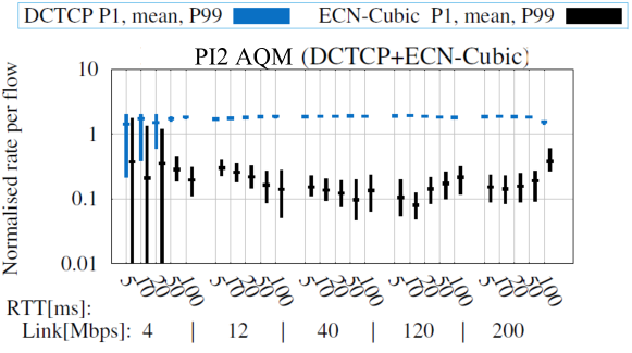
Figure 1: Quantification of the Rate Imbalance Problem between L4S and Classic ECN flows in a Classic ECN Queue. Flow rates are of long-running flows after a period of stabilization and normalized relative to precisely equal flow rates, 1 DCTCP vs. 1 ECN-Cubic, equal base RTTs, single queue PI² AQM; default parameters (see § 7.2 for full experiment details.)

Coexistence is only a problem if the bottleneck is a shared queue that supports Classic ECN marking. It is not known whether any shared queue Classic ECN AQMs are operational on the Internet, and so far no evidence has been forthcoming from the search for one. However, for L4S to proceed through standardization, it has to be assumed that such AQMs do exist or that they might exist. Therefore scalable congestion controls ought to respond appropriately if they detect a classic ECN AQM. In 2015, this was codified as one of the ‘Prague L4S’ requirements for scalable congestion controls, which have since been adopted by the IETF [DSBE20]. That requirement sets the problem that motivates the present report.

Other aspects of the L4S architecture already address coexistence in all the other possible cases, viz:

• If the bottleneck does not support any form of ECN (as is the case for the vast majority of buffers on the Internet), the only sign of congestion will be loss. It is easy to ensure that scalable congestion controls respond to loss in a Reno-friendly way, and all known scalable congestion controls do so (this is top of the list of “Prague L4S requirements” [DSBE20]).

• If the bottleneck applies per-microflow scheduling, it enforces coexistence without the need for the present algorithm. There are two sub-cases:

  • If there is a Classic AQM in each per-flow queue (understood to be a common deployment with FQ_CoDel [HJMT⁺18] and COBALT [PGI⁺19], which is used in CAKE), then the detection algorithm in the present paper ought to detect it and switch to Classic behaviour, which could provide performance benefits;

  • If the AQM in each per-flow queue supports L4S by detecting the L4S ECN identifier, then the full benefits of L4S will be available without the present algorithm, which will remain quiescent;

• If the bottleneck supports the DualQ Coupled AQM [DSBEW20], that will ensure that L4S and classic flows coexist and the full benefits of L4S will be available without the present algorithm, which will again remain quiescent.

2 Modular Approach

2.1 Modularity Requirements

An operator might want to determine the type of AQM on the path in-band, that is within live traffic, or out-of-band using test traffic.

An aim of in-band testing is to detect the type of AQM fast enough that a flow can start with the L4S behaviour but if necessary change over to Classic behaviour in the early stages of convergence.

However, a server operator might not want to trigger any change in behaviour. For instance, a CDN operator might want to use in-band or out-of-band testing purely to check the likelihood that the problem even exists over the paths they serve.

Therefore, a complete algorithm needs to work in two separable stages: detection then if necessary fall-back to Classic behaviour. More generally, fall-back ought to be called changeover because, as detection continues, the algorithm might need to reverse the change (either because the first change was premature, or because the bottleneck has changed).

Detection might purely measure the traffic’s characteristics (passive), or it might alter the way traffic is sent (active), e.g. altering send-timing, the sizes of certain packets, their markings, or adding extra probes. Active techniques tend to provide more certainty at the expense of altering live traffic. So passive detection is preferable at first, but if experimentation finds it is insufficient, active techniques could be kept in reserve as a double-check just before a changeover actually occurs, perhaps only in more challenging scenarios, e.g. high RTT, low link rate or when a bursty radio link appears to be present on the path.

Out-of-band testing is not applied to live traffic, so it can typically resort to active techniques straight away (unless it could potentially harm other live traffic).

The main body of this report is divided into the same modular sections; on passive detection (§ 3), active detection (both out-of-band in § 4 and in-band in § 5) and change-over (§,6). Different modules can then be mixed and matched to produce different solutions, one of which (so far) is evaluated in § 7.

2.2 Modular Code Structure

Beyond solving the coexistence problem, the following principles are proposed to structure the code for multiple purposes:

1. Rather than fall-back being a binary switch between modes, it should be a gradual changeover, the more certain it is that the AQM supports classic ECN;

2. Nonetheless, at either end of the spectrum of (un)certainty, there should be ranges where the CC behaves on the one hand purely scalably and on the other purely classically;

3. Minimal additional persistent TCP state;

4. The code should be structured with detection separate from changeover of behaviour, so that detection can eventually apply to more than one CC, while changeover is likely to be CC-specific;

5. However, until the concept is proven, it will be OK initially to implement the whole algorithm within the TCP Prague CC module, and only rationalize it once mature.

To simplify pseudocode, a float called c controls how much the CC should behave as classic, from 0 (scalable) to 1 (classic). In practice this might be an integer variable in the range 0 to CLASSIC_ECN. This will be driven from the variable classic_ecn, which is defined as the outputof the detection algorithm.

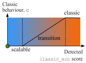
Figure 2: Score-based transition, rather than modal switch, between Scalable and Classic behaviour.

The classic_ecn indicator can continue beyond either end of this range. as depicted in Figure 2 and tabulated below, in order to implement a degree of stickiness where the CC algorithm behaves purely as L4S or purely classically.

-L_STICKY	$\leq$	classic_ecn	$\leq$	0	Pure L4S behaviour
0	$\leq$	classic_ecn	$\leq$	CLASSIC_ECN	Transition between L4S and classic
CLASSIC_ECN	$\leq$	classic_ecn	$\leq$	C_STICKY	Pure classic behaviour

It is up to the detection algo, not the CC algo, to maintain the classic_ecn variable. However, any particular CC algorithm can override the default parameters of the detection algorithm. For instance, a CC module could alter how ’sticky’ the hysteresis is at either end by overriding the default L_STICKY and/or C_STICKY parameters.

3 Passive Detection of Classic ECN AQMs

3.1 Candidate Metrics

The following metrics are likely to be relevant when detecting a classic ECN AQM:

• The onset of CE marking;

• Application-limited (no buffering at the sender);

• Receive window limited (rwnd $<$ cwnd);

• The moving mean deviation of the RTT (fbk_mdev) of the RTT.

• The difference between the smoothed RTT (fbk_srtt) and a minimum RTT (rtt_min), with suitable safeguards against a false minimum and against step changes;

• The distribution of the spacing between ECN marks

Note that the variable names fbk_mdev and fbk_srtt are prefixed with fbk_ to emphasize that they are specific to the fall-back algorithm, and not necessarily the same as the mdev and srtt variables that Linux TCP already maintains for its retransmit timer (see § 3.4).

3.1.1 Dependence on Presence of CE marking

Obviously no transition to classic should occur unless there has been a CE mark. Any transition should be suppressed for a number of RTTs after the onset of CE marking, both to allow the connection to stabilize and because aggressive competition for bandwidth is not a great concern with short flows. Indeed when rate ‘fairness’ is considered over time, it is more fair if long-running flows are less aggressive than short flows [GM02, Sd02, ZTH04, MSSM12, BCC⁺15, Bri19]—though a delay is sufficiently motivated by the need for a stabilization period rather than any desire to use a different form of fairness.

How long for instability to end?

A classical slow-start ends on the first CE (unless it had already ended due to a loss). In the next few rounds, all the flows suffer a period of instability as they recover from the transient overshoot of the new flow. The random nature of this period leaves them all at different shares of capacity. Then they might take a few hundred further round trips to converge on stable shares. It is likely that any flow-start approach developed for shallow threshold ECN might have a less clear cut transition between a flow-start phase and a period of convergence. Given this likely heterogeneity in approaches to flow-start, it is not feasible to quantify how long any single flow should wait after the first CE before starting to detect a classic ECN AQM, because the period of instability depends more on the behaviour of other flows than on its own behaviour.

Therefore it is proposed to start maintaining metrics as soon as the first feedback of a CE mark arrives, rather than attempting to wait for the subsequent instability to subside. As will be seen next, even if the RTT metrics start during this period of instability, they can be given plenty of time to stabilize before they alter the CC behaviour, while they remain scalable in the ‘sticky’ region.

How long before inappropriate convergence becomes significant?

In the original paper on TCP Cubic[HRX08], convergence was still described as ’short’ when it took one or two hundred rounds (assuming flows even last that long). Therefore, relative to overall convergence time, it will be insignificant if a flow takes a couple of dozen rounds to work out whether it should be converging to an L4S or to a classic target.

Rather than take an absolute number of rounds before the CC behaviour starts to transition, it would be better to depend on how strongly the other metrics are indicating that a transition is necessary. For instance, the higher RTT variance is, the fewer rounds would need to elapse before allowing a transition to start.

If CE marking stops for a protracted period, it will be likely that a non-ECN link has become the bottleneck. Then the choice between classic and scalable ECN behaviour would be moot and the default loss response would be sufficient. If CE marking were to pick up again later, it would be best to ignore (i.e. not measure) any period with more than one loss but no CE marking, then restart the detection algorithm if a CE mark ever appears again.

3.1.2 Dependence on being Self-Limited

If a TCP Prague flow is app-limited or receive-window limited (i.e. self-limited), there is no great need to fall back to classic behaviour on receipt of an ECN mark.

The presence of CE marks while the flow is not trying to fill the pipe (its send buffer is empty) probably implies that a greedy flow or other short flows are sharing the link. Then (assuming cwnd validation is being used) the flow will not be increasing cwnd as much as competing traffic could be. In that case, a large classic response to a CE-mark could under-utilize the link until cwnd returned. So a small scalable response would be more appropriate.

Also, any tendency towards classic behaviour due to RTT variability (see below) will be more due to other flows. So the classic ECN variable ought to reduce by a certain amount per RTT while a sender is self-limited. However, not being self-limited alone is not a reason to increase the variable—for that there has to be a positive sign of a classic ECN AQM, such as RTT variabiity.

Similarly, while the sender is idle, any previous detection of a classic ECN bottleneck could become stale. However, during an idle period there are no events to trigger any actions, so an adjustment to the classic ECN variable will have to be made at the restart of activity based on TCP’s idle timer.

3.1.3 Dependence on RTT Variability

A large degree of RTT variability is the surest way to detect a classic-ECN bottleneck. So, if accompanied by CE marking it is likely to imply a classic ECN AQM at the bottleneck. For the Internet, ’large variability’ can be quantified as more than about 1.5 ms of variability, given the target L4S delay will generally be 1 ms or less while the lowest target delay to which classic AQMs are recommended to be configured is about 5 ms. So any classic queue could vary from zero to slightly above that.

Pseudocode for dependence of classic ECN fall-back on RTT variability will be given in § 3.2. But first, the following two subsections will discuss possible false positives and false negatives.

Non-queuing causes of RTT variability with an L4S bottleneck

RTT variability can have other causes than queuing:

• A reroute.

• Variability in Interrupt handling, processor scheduling and batched processing by the endpoints and by nodes on the path.

Reroute:

A moving average of RTT and deviation of the RTT from this average does not filter out step changes in the base RTT (e.g. due to a reroute), which could cause the moving average to be temporarily ’incorrect’ so that the mean deviation from this incorrect average would temporarily expand (see Figure 13). The pseudocode in Appendix C is intended to fill that gap.

Other Non-Queue Variability:

The passive detection algorithm assumes that the combined result of all these variations will be small compared to variability of a classic ECN queue. This assumption has turned out to be sufficient in testing so far. But it will need to be tested in a wider range of scenarios and parameters altered accordingly (§ 3.6). If necessary active detection will need to be added, which is designed to complement passive detection where this assumption breaks down.

Low RTT variability with a classic ECN bottleneck

RTT variability will not distinguish a classic ECN bottleneck in the following cases:

• A high degree of flow multiplexing at a shared-queue bottleneck with a classic ECN AQM. The averaging effect of large numbers of uncorrelated sawteeth causes the mean deviation of the RTT of $N$ flows sharing a buffer to be about $1/\sqrt{N}$ of that of 1 flow, derived straightforwardly from the Central Limit Theorem [AKM04].

• …any others?

Few networks are designed so that sharing at a link serving a large number of individual flows is controlled by the end-points, let alone with a classic ECN AQM at this link as well. Nonetheless, we will consider three cases where this could possibly occur:

Commercial ISP’s access link with a shared-queue classic ECN AQM:

Invariably, the operator designs the network so that the bottleneck is in the access link allocated to each customer, the capacity of which is isolated from other customers using a scheduler. For the mean deviation of a flow to appear to be 5$\times$ lower (e.g. $800\,\mu$s rather than 4 ms), at least 25 classic flows would have to be multiplexed together, by the Central Limit formula above. Such a scenario can occur within a single customer’s access. However, for the fall-back algorithms of each flow to be fooled into thinking the bottleneck was L4S, that many classic flows would all have to run continually with no disruption from other flows. We have to accept that the algorithm could give a false negative in such a scenario, which is unlikely but possible.

Commercial ISP’s core or peering link with a shared-queue classic ECN AQM:

The bottleneck can sometimes shift to a core link or more likely a peering point, where there per-customer scheduling is unlikely to be deployed and flow multiplexing will be high enough to keep RTT very smooth. Usually this occurs during some sort of anomalous conditions, e.g. a provisioning mistake, a core link failure or a DDoS attack. If it does, the concern is that L4S flows could out-compete classic flows. Nonetheless, the scope for a high degree of flow rate inequality is very limited, as explained in Appendix D.

Campus network access link:

A corporate or University network is rarely designed with an individual bottleneck for each user. Rather, each user typically has high speed connectivity to the campus (e.g. 1Gb/s Ethernet) and all stations using the Internet at any one time bottleneck at the campus access link(s) from the Internet. In such an access link, L4S flows will not coexist well with classic flows (as in Figure 1). It is not known whether any campus networks use classic ECN AQM in their access link, but they might do. Until the operator of such an AQM can deploy an L4S AQM, an unsatisfactory work-round would be to reconfigure the AQM to treat ECT(1) as Not-ECT so that it uses drop not CE as a signal for L4S flows. However, this would disincentivize L4S deployment in the affected campus networks. The alternative of some campus networks just allowing the unfairness would also be an option (applications already open multiple flows to achieve a similar advantage in the access to existing campus networks).

3.1.4 Dependence on Minimum RTT

Minimum RTT metrics are known to be problematic, especially where the buffer is already filled by other traffic before a flow arrives. Therefore, it may be preferable not to use this metric at all, and rely solely on RTT variability.

Nonetheless, it would do no harm to use a min RTT metric, as long as the outcome was asymmetric. In other words, a large difference between fbk_srtt and srtt_min would make classic fall-back more likely, while a small difference would not make classic fall-back less likely. This is the approach taken in the pseudocode below.

Subsection Summary:

Figure 3 depicts the three main variables that will be used to drive Classic ECN AQM detection. It shows that queue variability should be able to increase or decrease the classic_ecn score symmetrically. In contrast queue depth will be limited to only increasing the score, due to the well-known problem of measuring a false rtt_min. The degree to which a flow is self-limiting is also asymmetric, but in this case it can only decrease the score.

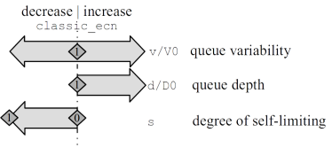
Figure 3: Visualization of the three main metrics, and how their effect on the classic_ecn score will be constrained

3.1.5 Dependence on Spacing Between ECN Marks

This metric was only first thought of after v2 of the algorithm had been implemented and evaluated. At present it is just an idea, but it seems the most promising approach. It might prove to be the only metric that is needed, which would provide a really simple solution. Otherwise, it would complement the other metrics above.

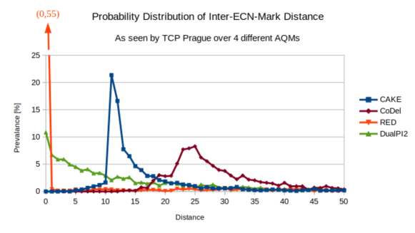
Figure 4: Distributions of spacing between marks for four different AQMs

The idea is to record the number of non-marked packets between one ECN mark to the next, and monitor the distribution of different spacings. At its simplest it might be sufficient to monitor the prevalence of just one selected spacing (e.g. 1, meaning a mark every other packet) relative to the total number of marks. The initial experiments shown in Figure 4 shoe that all the low spacings (except zero) are much higher for the L4S (DualPI2) AQM than the others, and there is fairly sound reasoning for that, as explained next.

By definition, all Classic AQMs filter out short term fluctuations in the queue. Most, if not all, known Classic AQMs also attempt to even out the spacings between the markings to avoid clustering—a process sometimes called derandomization. For instance: ‘

• After RED calculates the marking probability, to prevent marks clustering it converts the marking probability into a uniform random variable (see [FJ93, § 7]).

• CoDel [NJ18] and any AQM derived from it (e.g. COBALT [PGI⁺19]) uses a control law that inherently introduces a measured space between markings.

• PIE [PPP⁺13] and derivatives such as DOCSIS PIE [DOC19, Appx. M] use a derandomization algorithm similar to that of RED.

In contrast, by definition, an L4S AQM is specifically precluded from smoothing its markings [DSBE20, § 5.2], which is the job of the end system in the L4S architecture [DSBE20, § 4.4]. Therefore, typically the distribution of the spacings will be geometric. A geometric distribution has the counter-intuitive property that the greater the spacing, the less likely it will occur (much like the DualPI2 distribution in Figure 4). So the most likely spacing is always 0, the next most likely 1, and so on.

A higher prevalence of zero spacing is a special case, and not a useful distinguishing feature, because any AQM might occasionally mark all packets for a while when it overshoots.

Figure 4 is only an initial experiment based on single runs of 20s duration including flow startup with one link rate and one RTT (40 Mb/s, 20 ms) for two long-running flows started simultaneously; one Prague and one Cubic ECN.

It is very likely that the picture is less clear-cut in the Internet at large, although that will be hard to determine given no-one has yet captured a FIFO Classic ECN AQM in the wild, so we do not have one to dissect in the lab. Below some known complicating factors are discussed, some of which turn out not to be of concern, others need further investigation, and some are truly unknown and likely to remain so:

• Different L4S Distributions:

  • In a DualQ Coupled AQM, when there is a mix of L4S and Classic traffic, the L4S traffic is marked by coupling from an internal probability (termed $p^{\prime}$) pronounced p-prime, that also drives the Classic AQM. This would seem to mean that the distribution of spacing of L4S marks could be similar to that from the AQM in the Classic queue. However, on the Classic side, $p^{\prime}$ has to be squared then derandomized. While on the L4S side $p^{\prime}$ is merely factored up. So it would make no sense to derive the coupled L4S probability from the derandomized Classic probability, which would involve an unnecessary square root operation. This argument is very likely to apply whatever algorithm is used for the Classic AQM.

  • L4S AQMs often use a simple step threshold. So marking will not be driven from a random variable, and therefore it will not follow a geometric distribution. A pure step threshold is likely to cause its own distinctive distribution of spacing, with long runs of solid marking followed by long runs of none. However, different patterns are likely to result from different levels of short flows in the background.

• Different Classic Distributions (assuming FIFO Classic ECN AQMs do exist):

  • Even if a Classic ECN AQM derandomizes marking in a FIFO, it only derandomizes the spacing between marks in the aggregate, not in each flow. If there are multiple flows the packets from each flow tend not to take perfect turns as they arrive, so the spacing between markings in each flow becomes more random again (it un-derandomizes) [Bri15, § 5.6]. This could start to look more like the distribution of spacing from an L4S AQM.

  • It is possible that some Classic ECN AQMs will not include derandomization code, for instance in high-speed switches to simplify the hardware process.

  • Large numbers of AQM designs have been proposed in research literature and in patents. If any were implemented, they might not all have included derandomization.

If further experimentation proves that the spacing between marks still has merit as a metric, it will need to be designed into an algorithm that increases the classic_ecn variable the more likely the AQM is Classic. And it will need to take account of periods when the flow might be application limited, receive-window-limited or idle. However, as already explained, the algorithm described below was designed implemented and tested before using an inter-mark spacing metric had been thought of.

3.2 Passive Detection Pseudocode

The following pseudocode pulls together all the passive detection ideas in the preceding sections.

/* Parameters */
#define V 0.5          // Weight of queue *V*ariability metric
#define D 0.5          // Weight of mean queue *D*epth metric
#define S 0.25         // Weight of *S*elf-limiting metric
#define C_FRAC_IDLE 2  // Multiplicative reduction in classic_ecn each idle timeout
#define CLASSIC_ECN 1 // Max of transition range for classic_ecn score
#define L_STICKY 16*V  // L4S stickiness incl. min rounds from CE onset to transition
#define C_STICKY 16*V  // Classic stickiness
#define V0 750         //  Reference queue *V*ariability [us]
#define D0 2000        // Reference queue *D*epth [us]

/* Stored variables */
classic_ecn; // Signed integer. The more +ve, the more likely it’s a classic ECN AQM
rtt_min;    // Min RTT (using Kathleen Nichols’s windowed min tracker in Linux)
fbk_srtt;           // The smoothed RTT (see later pseudocode)
fbk_mdev;           // The mean deviation of the RTT (see later pseudocode)
s;           // Proportion of the latest RTT that was self- (app- or rwnd-) limited

// Temporary variables to improve readability
v = fbk_mdev;
d = fbk_srtt - rtt_min;           // The likely mean depth of the queue.
delta_;

/* The following statements are intended to be triggered by the stated events */

{   // On connection initialization
    classic_ecn = -L_STICKY;
}

{   // On CE feedback, enable delta_ calc’n if classic_ecn is clamped at its minimum
    classic_ecn += (classic_ecn <= -L_STICKY);
}

{    // On expiry of idle timer
    if (classic_ecn > 0) {
        classic_ecn = classic_ecn/C_FRAC_IDLE;
        re-arm_idle_timer();
    }
}

{   // Per RTT
    if (classic_ecn > -L_STICKY) {    // Suppress delta_ calc’n if classic_ecn at min
        delta_ = V*lg(v/V0) + D*lg(max(d/D0, 1)) - S*s;
        classic_ecn = min(max(classic_ecn  + delta_, -L_STICKY), C_STICKY);
    } else {
        ect_tracers = 0;    // Unsuppress ect_tracers (for active detection in Section 5)
    }
}

{   // Per ACK
    // Update fbk_mdev and  fbk_srtt (see later pseudocode)
}

Passive Detection Pseudocode Walk-Through

While classic_ecn sits at -L_STICKY, calculation of delta_, the change in classic_ecn, is suppressed to save unnecessary processing. Maintenance of the variables used in this calculation could also be suppressed (not shown).

At connection initialization, maintenance of the classic_ecn variable starts off in the above quiescent state. Feedback of a CE mark awakens it by incrementing classic_ecn by its minimum integer granularity (1).

Every RTT, as long as classic_ecn is not in its quiescent state, the per-RTT change in classic_ecn is calculated. This is the core of the passive classic ECN detection algorithm. To aid readability, a temporary variable (delta_) is assigned to this intermediate calculation.

The change in classic_ecn consists of three terms, each weighted relative to each other by the three parameters V, D and S:

RTT Variability, v (§ 3.1.3):

The metric lg(v/V0) is used, where lg() is an approximate (fast) base-2 log (see Appendix B.2) and V0 is a reference mean-deviation parameter (default $750\,\mu$s). It is increasingly hard to achieve smaller deviations, so it is necessary to use a log function in order to ensure that a mean deviation of, say, $23\,\mu$s moves the classic ECN variable as much downwards as a mean deviation of 24 ms moves it upwards (respectively 32 times smaller and 32 times larger than V0 = $750\,\mu$s).

Likely Mean Queue Depth, d (§ 3.1.4:

The metric lg(max(d/D0), 1) uses the log of the ratio of d over the reference queue depth D0 for the same reason as the previous bullet. However, the max() with respect to 1 ensures it ignores queue depths below the threshold, which could be suspect, as explained in § 3.1.4.

Self-Limitation, s (§ 3.1.2):

Here the fraction of the RTT that was self-limited can be used directly.

The last two variables can each only push classic_ecn in one direction (see Figure 3). Mean queue depth can only push it upwards (more classic), while self-limitation can only push it downwards (less classic). If mean queue depth is below the reference queue depth D0, or there is no self-limitation in a round, the classic_ecn indicator remains unchanged.

If, on balance, the calculations to detect classic ECN AQM are positive, delta_ increases classic_ecn towards its maximum (C_STICKY). But if they are negative, delta_ decreases classic_ecn towards its minimum (-L_STICKY) where further calculations will be suppressed, at least until calculations are reawakened by the next CE mark.

During an idle period, classic_ecn is exponentially reduced by default to 1/2 of its previous value on every expiry of the idle timer, but only if it is positive. Thus, while idling, a connection that had detected a classic ECN AQM will gradually drift to the L4S end of the transition, but towards the cusp of the transition. Then, if it continues to detect a classic ECN AQM once it restarts, It will immediately transition to classic ECN mode again, while it is restarting.

3.3 RTT Smoothing

The smoothed RTT and the mean deviation from that smoothed RTT are the primary metrics used by the passive classic ECN AQM detection algorithm. They both use exponentially weighted moving averages.

All implementations of TCP already maintain two such variables; the EWMA of the RTT and an EWMA of the mean deviation of RTT samples from that smoothed RTT. In Linux, they are called srtt and mdev and both are updated on every ACK. It was originally hoped to reuse these variables for classic AQM detection. However, they are unsuitable for two reasons:

• TCP maintains srtt and mdev for calculation of its retransmission time out (RTO). For this it needs a worst-case measure of the duration between sending a packet and seeing an ACK. So, whenever TCP receives an ACK, it measures the RTT for RTO purposes (mrtt) from when it sent the oldest newly acknowledged packet. This includes the duration of the delay introduced by the receiver’s delayed ACK mechanism, making these metrics unusable as a smoothed measure of the actual RTT. The presumption that RTT is used for RTO calculation is also built into the time the receiver is expected to stamp into TCP’s time-stamp option, making timestamps unusable for measuring actual round trip delay as well.

• In Linux, TCP smooths these variables (srtt and mdev) over very few ACKs (8 and 4 respectively) whereas, for classic ECN AQM detection, ideally RTT needs to be smoothed over at least one sawtooth of the flow’s own window, in order to pick up the full depth and variability of the bottleneck queue.

Terminology: After $g$ iterations, a step change in an EWMA’s input will have changed the moving average by about 63% of the step, or precisely $1-1/e$, where $e$ is the base of the natural logarithm. This is what the phrase smoothed ‘over’ a certain number of iterations means. It is another way of saying that the smoothing gain of the EWMA is $1/g$. For instance, saying that TCP smooths srtt over 8 ACKs, is alternative way of saying the smoothing gain is 1/8. The smoothing gain of an EWMA is the fraction of each newly measured value that is added to the average on every update (and the fraction of the old average that is subtracted).

In the original discussion of RTO estimation in Jacobson and Karels [JK88, Appx A] the EWMAs for srtt and mdev were recommended to be smoothed over respectively a little greater and a little less than the congestion window, measured in segments. However, the Linux code has never related these parameters to cwnd and they remain hard coded as they were when typical values of cwnd were hundreds of times lower than they are today.

Linux already maintains a more precise RTT metric on each ACK. It stores the times at which it sends every packet and it measures a variable we shall call acc_mrtt from the time at which it sent the packet that elicited the ACK to when it receives the ACK.

It is not costly to maintain an extra pair of EWMAs based on this more precise acc_mrtt variable. However, it is necessary to detect queue variations over the timescale of TCP’s sawteeth, which requires smoothing over a very large number of ACKs; far more than the 4 or 8 currently used in Linux and other OSs for RTO calculation.

Appendix A addresses the question of how many ACKs to smooth over. The theoretical number of ACKs in a Classic sawtooth is $(\texttt{ssthresh})^{2}$. However, the appendix explains that this can be considered as a rare upper limit. In practice the sawteeth of Classic congestion controls rarely reach this size, especially in the presence of other traffic, such as short flows.

In experiments with a range of link rates between 4 Mb/s and 200 Mb/s and RTTs between 5 ms and 100 ms, the formula that resulted in a good compromise between precision and speed of response was:

$$\mathtt{fbk\_g\_srtt}=2*(\mathtt{ssthresh})^{3/2}.$$

And the mean deviation is smoothed twice as slowly as the RTT itself, i.e.:

$$\mathtt{fbk\_g\_mdev}=\mathtt{fbk\_g\_srtt}*2.$$

color=olive!40,inline]Bob: Currently, the Linux code uses g_mdev = g_srtt * 2, but I would like to try g_mdev = g_srtt and even g_mdev = g_srtt / 2

3.4 RTT Smoothing Pseudocode

// fbk_g_srtt = U2 * (ssthresh)^(U1)
#define U1 (3/2)
#define U2 2
#define FBK_G_RATIO 2    // fbk_g_mdev = fbk_g_srtt *  FBK_G_RATIO

/* Stored variables */
fbk_srtt;                // Smoothed RTT
fbk_mdev;                // Mean deviation
fbk_g_srtt;              // srtt gain (initialized dependent on ssthresh)
fbk_g_mdev;              // mdev gain (initialized dependent on ssthresh)

/* Temporary variables */
u32 acc_mrtt;            // Measured RTT from newest unack’d packet
s64 error_;

{   // At start of connection, either after first RTT measurement or from dst cache
    fbk_srtt = acc_mrtt;
    fbk_mdev = 1;        // No need for conservative init, unlike for RTO
}

{   // Per ACK
    // Update EWMAs
    error_ = acc_mrtt - fbk_srtt;
    fbk_srtt += error_  /  fbk_g_srtt;
    fbk_mdev += (abs(error_) - fbk_mdev) / fbk_g_mdev;
}

{   // Per ssthresh change, including when initialized
    fbk_g_srtt = U2 * ssthresh^U1
    fbk_g_mdev = fbk_g_srtt * FBK_G_RATIO
}

RTT Smoothing Pseudocode Walk-Through

The EWMAs in the ‘Per ACK’ block are straightforward. The mean deviation is defined as the EWMA of the non-negative error, so it is calculated using the abs() function, which returns the absolute (non-negative) value of its argument.

In the ‘Per-ssthresh change’ block, the gains used for the EWMA are adjusted to maintain their relationship with ssthresh as just explained in § 3.3.

Appendix A gives more detailed pseudocode based on that above, to address the questions of EWMA precision and upscaling when using integer arithmetic in the kernel.

3.5 Questioning Assumptions used for Passive Detection

3.5.1 Clocking Interval for classic_ecn

So far, it has been assumed that classic_ecn should be recalculated once per RTT, for all the detection metrics except idling time. The question of which event is appropriate to update this variable needs to be addressed explicitly.

Four potential intervals on which to clock changes are:

• round trips

• absolute time intervals

• after a certain amount of sent packets, or even sent bytes

• after a certain amount of feedback (ACK counting).

Stabilization and convergence:

It makes sense to count how long to wait for a connection to stabilize and converge in round trips, because each flow adjusts iteratively on a round trip timescale.

RTT variability:

There is an argument that changes to classic_ecn due to RTT variability should be clocked on a count of the ACKs received, e.g. every 32 or every 64 ACKs. This is because the precision of round trip smoothing and measurements of mean deviation depends on how many ACKs have contributed to the average. However, the variability of the queue itself alters dependent on evolution of each flow’s congestion window, which adjusts on a round trip timescale. Therefore dependence of the value of classic_ecn on RTT variability metrics should be clocked against round trips.

Self-limitation:

Self-limitation is measured as a proportion, so it does not matter whether it is a proportion of a round, a proportion of a certain time period, or a proportion of any other metric. Given other metrics should be clocked on round trips, it makes sense to clock self-limitation calculations on the same events.

Idling:

There is no basis to argue that changes to classic_ecn due to idling should be clocked on any particular metric. Nonetheless, the only metric that continues to clock during an idle period is time, so this is the only practical metric to use.

Counting either in sent packets or absolute time would be easy to implement, but neither seem to have any logical backing, for any of the metrics.

3.5.2 Clocking Interval for RTT EWMAs

Appendix A addresses the question of how many ACKs to smooth the RTT EWMAs over. However, it does not question whether these EWMAs should be or need to be updated on every ACK, particularly given the gain has to be so tiny, which implies that less frequent updates with a larger gain would be no less precise but less costly in processing terms.

It would be possible to measure the RTT of only a sample of ACKs, and increase the gain accordingly. However, this would involve extra complexity, and the actual additional processing cost is only 4 adds, 2 bit-shifts and a compare per ACK (see Appendix A), which is not particularly problematic. Sampling has its own complexity because the sampling ratio would have to be adaptive, in order that it could revert to 100% when the number of ACKs per round trip was small. It would also require an extra state variable to be maintained per ACK, in order to record when the next sample was due.

Therefore, on balance it has been decided to maintain the EWMAs of RTT and mean deviation per ACK. But there is nothing to stop other implementers using sampling.

3.6 Parameter settings

The parameters currently given in the passive detection pseudocode (§§ 3.2 & 3.4) are heuristics arrived at as a result of a large number of calibration experiments over a testbed with link rates of 4–200 Mb/s and RTTs of 5–100 ms. Higher link rates could have been included, but the most challenging part of the range is the low end. § 7 summarizes the results of evaluations using the parameters resulting from these calibration experiments.

The current set of parameter values has solely been informed by experiments with CoDel [NJ18] as the Classic AQM and DualPI2 [DSBEW20] as the L4S AQM (both with default settings). CoDel was chosen given it is a good candidate for the worst-case for the fall-back algorithm to detect, for two reasons:

• CoDel’s default setting of target is very low (5 ms). This pegs its queue delay low relative to other Classic AQMs and tends to cause under-utilization for all but the lowest RTTs. Both these factors lead to very little, if any, queuing delay. This makes CoDel more difficult to distinguish from an L4S AQM, and therefore likely to be a worst-case from a parameter-setting viewpoint.

• CoDel’s design is highly specific to Classic congestion controls, probably exhibiting the slowest response of all AQMs to the high levels of ECN signalling induced by scalable congestion controls [PGI⁺19].

As the algorithm is evaluated with other AQMs, it may be necessary to tune the parameters further.

4 Out-of-Band Active Detection ‘of Classic ECN AQMs

Out-of-band testing presents few constraints on the traffic patterns that can be used. So it is possible to use unsubtle approaches like running two flows in parallel, which is described here.

A server could be set up with ECN enabled so that, when a test client accesses it, it serves a script that gets the client to open two parallel long-running flows. Then it could serve one with a Classic CC (that sets ECT(0)) and one with a scaleable CC (that sets ECT(1)).

If neither flow induces any ECN marks, it can be presumed the path does not contain a Classic ECN AQM.

If either flow induces some ECN marks, the server could measure the relative flow rates and round trip times of the two flows. Table 1 shows the AQM that can be inferred for various cases.

Rate	RTT	Inferred AQM
$L>C$	$L=C$	Classic ECN AQM (FIFO)
$L=C$	$L=C$	Classic ECN AQM (FQ)
$L=C$	$L<C$	FQ-L4S AQM
$L\approx C$	$L<C$	DualQ Coupled AQM

Table 1: Out-of-band testing with two parallel flows, showing those cases with some ECN marks apparent. L=L4S, C=Classic.

The power of this approach is that is can identify whether a Classic ECN AQM is in a FIFO (which is the type being sought), or in an FQ scheduler (which is not).

In the case of the DualQ Coupled AQM, the relative rates will depend on the configuration, so they are only shown as ’$\approx$’. Other combinations of outcomes are theoretically possible, e.g. $L>C$ for RTT, but the test would have to be abandoned in such cases, because no known AQM would cause such an outcome.

5 In-Band Active Detection of Classic ECN AQMs

5.1 In-Band Active Detection: ACK Problems in TCP

When active detection is used in-band, by definition it alters the traffic. So care has to be taken not to intrude too much into live sessions.

The most likely testing pattern would be to start with passive testing, then only introduce a little active testing before changing the CC behaviour, particularly if the results were not clear cut. This is the approach expected for Solution No.1 (§ 5.2). Alternatively, active testing could be used on a small sample of flows, which is the most likely approach to be taken for Solution No.2 (§ 5.3).

We start out on the assumption that an L4S sender will set some packets within a single flow to ECT(0) even though it should set them to ECT(1). In Solution No.1 the sender checks for differences in RTT. In Solution No.2 it checks for differences in marking.

One can imagine a number of naïve active measures that a sender could take:

• It could duplicate a small proportion of ECT1 packets and set them as ECT0.

• it could set a small proportion of packets to ECT0 instead of ECT1;

We shall call these ’ECT tracer’ packets, because they trace whether the ECT field causes a packet to be classified into a different queue. However, if TCP is being used, and if the receiver was using delayed ACKs (most do), it would confound these naïve approaches:

• in the first case, even if both duplicates were acknowledged (the first to arrive might not be), the sender would not be able to tell from the acknowledgement(s) which duplicate had arrived first.

• In the second case, some ECT0 packets would not trigger an ACK so their delay could not be measured. Also, if the bottleneck were an L4S DualQ Coupled AQM, any queuing delay suffered by the ECT0 packets would hold back the connection, and some might be delayed enough relative to ECT1 packets to make TCP believe they had been lost, causing the sender to spuriously retransmit and spuriously reduce its congestion window.

5.2 In-Band Active Detection: Solution No. 1

5.2.1 Active Solution No. 1: Approach

A better strategy would be:

• for the sender to make the receiver override its delayed ACK mechanism by ensuring that at least part of both tracer packets duplicates bytes already sent. This is because standard TCP congestion control [APB09, APS99] recommends that a receiver sends an immediate ACK in response to duplicate data to expedite the fast retransmit process, and this recommendation has stood since the first Internet host requirements in 1989 [Bra89].

• for either tracer packet to push forward the acknowledgement counter, so that the sender can tell which probably arrived first (there can be no certainty, because ACKs can be reordered).

The best sender-only strategy so far conceived would be as follows (also illustrated in Figure 7):

1. If, during passive testing, the classic_ecn indicator is approaching the transition range from below, i.e. negative but close to zero, for a small proportion of segments send instead the following three smaller packets, all back-to-back:

   • a larger front segment marked ECT1;

   • a smaller middle segment marked ECT0, duplicating at least the last 2 B of the first segment;

   • a rear segment marked ECT1 of the same size as the second but only duplicating the last byte of the first segment;

2. If the ACK for the middle tracer arrives after that for the rear tracer, the AQM is likely to be L4S (unless some other mechanism happens to have coincidentally re-ordered the packet stream at this point);

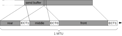
Figure 5: Tracer packets to detect separate treatment of ECT1 packets

Note that the ECT0-marked packet only includes redundant bytes, so if it is delayed (or dropped) by a classic queue, it does not degrade the L4S service.

The combined size of all three packets should be no greater than 1 MTU so that, if packet pacing is enabled, all three packets will remain back-to-back without having to alter pacing (also the two back-to-back ECT1 packets will cause no more of a burst in an L4S queue than a single packet would).

The front packet is larger to reduce the risk that detection of L4S AQMs will sometimes fail. Being larger, it is more likely to still be dequeuing when the rear packet arrives at the bottleneck. Otherwise, if there was a DualQ Coupled AQM at the bottleneck, and if there was no other classic traffic queued ahead of the middle tracer, it could start dequeuing after the front packet had dequeued, but before the rear tracer arrived.

Nonetheless, in order to minimize the possibility that the small tracer packets are treated differently by middleboxes, they should be larger than the size $S$ of the largest packet that might be considered ’small’ by common acceleration devices ($S=98$ B would probably be sufficient).

color=olive!40,inline]Bob: ToDo: Write up a symmetric facility at the classic end of the spectrum. And write-up pseudocode in the following section, including a way to take multiple active measurements and act on their combined outcome.

5.2.2 Active Solution No1̇: Pseudocode

The following pseudocode implements the active detection ideas in § 5.2.1. It uses some of the macros and variables defined in the passive detection pseudocode above.

// Parameters
#define TRACER_NUM 4    // Number of sets of 3 active tracers to send
#define REAR_SIZE 98    // Min size of middle and rear tracers [B]

ect_tracers = 0;  // Unsigned int storing remaining tracers (-ve means disarm sending)
tracer_nxt = 0;   // Point in the sequence space after the most recently sent tracer
                  // special (tracer_nxt == 0) disables checking for tracer ACKs

// Functions
send_tracer(start, size, ecn);    // Sends ECT tracer seg from ’start’ in send buffer

// The following statements are intended to be inserted at the stated events

{   \\ Per RTT
    if (classic_ecn >= -L_STICKY/TRACER_NUM && !ect_tracers) {
        ect_tracers = TRACER_NUM;
    }

    if (ect_tracers < 0)    // The tracer armed 1RTT ago has been sent
        ect_tracers *= -1;    // Arm sending of the next tracer
}

{   // Prior to sending a packet
    if (ect_tracers > 0 && snd_q >= smss) {
        front_size = smss - 2 * (sizeof_tcp_ip_headers() + REAR_SIZE);
        send_tracer(snd.nxt,                 front_size, ECT1);    // Front tracer
        send_tracer(snd.nxt - 2,             REAR_SIZE,  ECT0);    // Middle tracer
        send_tracer(snd.nxt - REAR_SIZE + 1, REAR_SIZE,  ECT1);    // Rear tracer
        tracer_nxt = snd.nxt;
        if (--ect_tracers) {
            ect_tracers *= -1;    // Negate to disarm sending of the next tracer
        } elif (classic_ecn >= -L_STICKY/TRACER_NUM) {
           ect_tracers -= TRACER_NUM + 1;    // Suppress further tracers
        }
    }
}

{   // On receipt of seg (pure ACK or data)
    if (tracer_nxt) {
        if (rcv.nxt == tracer_nxt && seg.sack == tracer_nxt - 1)
            // middle arrived after rear, so probably L4S bottleneck
            classic_ecn = max(classic_ecn - L_STICKY/TRACER_NUM, -L_STICKY);
        if (ect_tracers == -TRACER_NUM - 1)    // Further ECT tracers have been suppressed
            tracer_nxt = FALSE;    // Suppress further ACK checking
    }
}

Interaction between Active Testing and the classic_ecn Indicator:

Greater RTT variability during passive testing might imply either a classic bottleneck or an L4S bottleneck combined with variability from another link (e.g. non-L4S WiFi). Whereas low variability is more likely to imply an L4S bottleneck. Therefore if the result of an active test is L4S, it pushes the classic_ecn indicator towards the L4S end, counteracting the pposite trend due to variability. Whereas if the result of an active test is classic, it does not need to alter classic_ecn; it can leave variability to do that.

Active detection is more decisive, but it alters the normal transmission pattern. So to avoid unnecessarily altering the sending pattern, passive measurement alone is used first to determine whether active measurement is worthwhile.

If active measurement proves necessary, the plan then is to send a small number (default TRACER_NUM = 4) of sets of three tracer packets. If any set of tracers detects that an L4S AQM is likely, it moves the classic_ecn indicator towards the L4S end of the spectrum by an amount L_STICKY/TRACER_NUM.

Thus if all 4 tests detect L4S, classic_ecn reduces by L_STICKY. The tests start at classic_ecn >= -L_STICKY/4, so if all 4 tests detect L4S, it will return to its floor value of -L_STICKY, and the CC will never have behaved as anything other than pure L4S. Bear in mind that the classic_ecn indicator will still be altered by the passive detection algorithm as well.

If, on the other hand, no set of tracers detects L4S, the active tests will not alter the classic_ecn indicator at all. Then, if the bottleneck is classic, continuing passive tests will detect the higher RTT variability and continue to push the classic_ecn indicator towards the classic end of the spectrum.

Between these two extremes, if not all the active tests detect L4S, the classic_ecn indicator will be pushed down less and stop short of its floor. Then if RTT variability continues, passive detection will more rapidly return it to the -L_STICKY/4 threshold where active tests resume.

State Variables

To detect which tracer packet arrived first, it is necessary to store an indication of which feedback to check. Therefore no more than one set of tracers is sent per round trip, to minimize the per-connection state needed. This also spaces out the tracer tests, so that the small amount of redundant data each one sends hardly causes any inefficiency.

Two additional state variables are needed for each connection:

• ect_tracers: This state variable stores the number of ECT tracers outstanding. Zero is not really a special value; it just has the expected meaning—that no tracers are outstanding.

• tracer_nxt: After a set of three tracer packets have been sent, tracer_nxt stores the next byte in the sequence space. Then later the matching ACKs for the tracers can be found. If the ACK never arrives, there is just no outcome to the test.

Negative values of ect_tracers are special; they store the number of outstanding sets of tracers but disarm them for a round trip (so that the feedback from the last one has time to return).color=olive!40,inline]Bob: There could be a race condition here, where the variable will be needed for the next tracer before it has been used to pick up the feedback from the last one.

The negative value of ect_tracers one lower than -TRACER_NUM (-5 by default) is a further special value that suppresses all further tracers.

Tracers are not suppressed as long as the outcome after 4 tracers has reduced the classic_ecn indicator below the threshold at which active tests are triggered (-L_STICKY/4). Then, if the indicator rises to this threshold again, another set of tracers can be triggered. But, if the indicator has not reduced after the 4 tracer tests (i.e. all 4 tracer tests pass without reordering), all further active tests are suppressed so that continuing passive measurements are allowed to push the indicator upwards towards the classic ceiling (causing the CC to transition to classic behaviour).

If RTT variability reduces (e.g. because the bottleneck moves from a classic to an L4S AQM) such that the passive tests on their own pull the indicator down to the L4S floor, active tests suppression is removed by setting ect_tracers = 0.

Per Packet Processing Efficiency

The special values of the variables ect_tracers and tracer_nxt are used to suppress the more complex conditions that would otherwise have to be checked per packet, respectively: whether each packet to be sent should be replaced by a set of tracers; and whether each ACK is feedback from a tracer.

For efficient implementation, rather than checking a flag variable on millions of packets just to send or receive a few packets differently, it might be better to somehow suppress regular packet sending, send the required number of tracer packets manually, then resume sending. This will need to be investigated during implementation.

5.3 In-Band Active Detection: Solution No. 2

5.3.1 Active Solution No. 2: Approach

To date, the draft text of the experimental IETF RFC to specify the L4S markings says:

   For backward compatibility in uncontrolled environments, a network
   node that implements the L4S treatment MUST also implement an AQM
   treatment for the Classic service as defined in Section 1.2.  This
   Classic AQM treatment need not mark ECT(0) packets, but if it does,
   it will do so under the same conditions as it would drop Not-ECT
   packets [RFC3168].

It has been suggested that this could be amended to preclude any Classic AQM from marking ECT(0) packets if it is coupled with an L4S AQM. Then, an L4S source could detect a Classic ECN AQM by probing with ECT(0) packets to see if they were marked. In the following, this will be termed exclusive marking.

With a flow-queuing (FQ) scheduler, an L4S and a Classic AQM can both be applied within each queue [HJMT⁺18, § 5.2.7] by applying immediate ECT(1) marking at a shallower threshold. It has also been suggested that it would not be necessary for the whole FQ system to choose between L4S and Classic ECN. Instead, within each per-flow queue (FQ), the queue could continue to support Classic ECT(0) marking, except it could be required not to mark ECT(0) packets if the same queue had ‘recently’ seen an ECT(1) marking. In the following, this will be termed FQ-exclusive marking.

‘Recently’ could mean in the lifetime of the per-flow bucket, or after a timeout. If the timeout option were chosen, it would require at least a 2-bit counter per queue. The timeout could be implemented by initializing each counter to zero, then setting it to 3 on every ECT(1) packet. Then a timer shared over all queues could decrement all the counters at a regular interval, $T$. ECT(0) marking would be disabled in any queue with a non-zero counter, so the timeout would last for at least $2T$ and at most $3T$.

The whole ‘Solution No.2’ approach would still work even if some FQ AQMs supported both L4S and Classic AQMs but did not implement FQ-exclusive marking (important given such AQMs are already deployed). This is because the queue for a flow with decent proportion of ECT(1) packets would tend to sit below the shallow ECT(1) threshold and never reach the deeper point where ECT(0) marking started.

A notable benefit of the exclusive marking idea is that it only needs to be temporary, for instance during the early stages of the experimental phase of L4S. If it proves not to be useful, perhaps because some better approach is developed, the standards can be updated and Classic ECN AQMs can be allowed to mark ECT0 packets alongside L4S ECT1 marking.

The following two test strategies have been proposed to exploit exclusive marking, if it were standardized:

ECT0 probes:

One approach would be to intersperse small ECT(0) probe packets within an L4S ECT(1) flow, while attempting to induce enough congestion for some of these probe packets to be likely to be dropped or marked. Then if any ECT(0) packets were marked it would be highly likely that there was a Classic ECN AQM at the bottleneck.

Late onset ECT1 stripe:

In this approach, a long-running flow would start with all ECT0 packets. Then after some congestion had been induced (CE marking or loss), a small proportion of packets (e.g. 5%) would be marked ECT1 while the majority would continue as ECT0.

More details of each strategy including pros and cons are discussed below. It is uncertain whether either would be considered acceptable for in-band testing; ECT0 probes might be too slow, and the late onset ECT1 stripe might not be sufficiently benign. However, other strategies might be developed.

ECT0 Probes:

This approach relies on being able to tell whether specific packets have been ECN-marked. Therefore, if it were used over a TCP connection, a technique similar to that in § 5.2.1 would be needed to avoid the sender being confused by delayed ACKs.

Although a marking on any ECT0 probe would prove that a Classic ECN AQM was likely, absence of such a marking would not prove absence of a Classic ECN AQM. If the ratio of ECT0 probes to ECT1 packets was $1:P$, then the test would have to continue until the number of ECT1-marked packets had exceeded some multiple of $P$, e.g. $m*P$ (say $m=10$, to improve the chances. This would only be reliable if the flow and its ECT1 marking was steady and regular. Actually the number of ECT1 packets would have exceed $m*r*P$, where $r$ is the ratio of the largest to the smallest packet size used by some AQMs to biasing marking towards larger packets. Although deprecated by IETF RFC 7141, some common AQMs adopt this practice, for instance DOCSIS PIE [WP17, § 4.6].

Late onset ECT1 stripe:

This approach would offer typical Classic queue delay even if the bottleneck AQM supported L4S. So it would have to be used sparingly on a small sample of flows, perhaps to characterize the paths to different destinations (or for out-of-band tests). Given L4S connections are designed to fall back to Classic ECN or no ECN at all where it is only partially deployed, occasional flows without L4S support should be unremarkable, particularly during the experimental phase of L4S.

Table 2 shows the various patterns of marking that might result from this test, and what could then be concluded about the bottleneck in the right-hand column.

$\begin{array}[]{|crrc|crrcrrc|l|}\hline\cr\vrule\lx@intercol\hfil\textrm{All ECT0}\hfil\lx@intercol\vrule\lx@intercol&\vrule\lx@intercol\hfil\textrm{95\% ECT0}\hfil\lx@intercol&&\lx@intercol\hfil\textrm{5\% ECT1}\hfil\lx@intercol\vrule\lx@intercol&\\ \cline{2-3}\cr\cline{6-7}\cr\cline{9-10}\cr&\textrm{drop}&\textrm{mark}&&&\textrm{drop}&\textrm{mark}&&\textrm{drop}&\textrm{mark}&&\textrm{The implied type of bottleneck}\\ \hline\cr&>0&0&&&>0&0&&>0&0&&\textrm{Tail-drop or Non-ECN AQM (FQ or FIFO)}\\ &&>0&&&&>0&&&>0&&\textrm{Classic ECN AQM (FQ or FIFO)}\\ &&>0&&&&>0&&&\approx 1&&\textrm{FQ-L4S AQM (non-exclusive)}\\ &&>0&&&>0&0&&&>0&&\textrm{FQ-exclusive L4S AQM}\\ &>0&0&&&>0&0&&&>0&&\textrm{DualQ L4S AQM}\\ \hline\cr\end{array}$

Table 2: Possible patterns of marking resulting from ‘Late Onset ECT1 Stripe’ testing. An empty cell means ‘don’t care’.

A run would have to be aborted under the following conditions:

• If no congestion indication (drop or marking) can be induced on an ECT0 packet, either before ECT1 packets are introduced or after, the run has to time out;

• Whether or not there are congestion indications on any ECT0 packets, a run has to eventually time out if there is never a congestion indication on an ECT1 packet;

• If any ECT0 packet has been marked, a run has to eventually time out if no ECT1 packet is ever marked;

• If no ECT0 packet is marked before ECT1 packets are introduced, but an ECT0 packet is marked after, the run has to abort.

6 CC Behaviour Changeover Algorithm

6.1 TCP Prague-Based Example

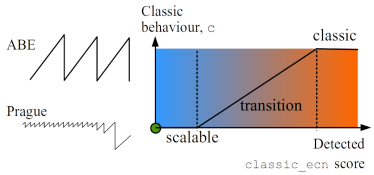
Figure 6: Visualization of the Transition between Scalable and Classic behaviour.

The proposed changeover algorithm transitions its response to ECN from scalable to ABE-Reno as c transitions from 0 to 1, as visualized in Figure 6.

Alternative Backoff with ECN (ABE) is an Experimental RFC [KWAF18] that suggests it is preferable for the reduction in cwnd to be less severe in response to an ECN signal than to a loss. The logic is that loss is more likely to emanate from a deep buffer, whereas any ECN signals are likely to be emanating from a modern AQM which will be configured with shallow target queuing delay. Therefore, it is reasonable to reduce less in response to ECN in order to improve utilization. A downside with ABE is that it will lead to ECN flows competing more aggressively with non-ECN flows, but the difference is not so great that non-ECN flows would be severely disadvantaged.

It is easiest for TCP Prague to fall back to Reno or ABE-Reno (though falling back to a less lame congestion control such as Cubic or BBRv2 would be preferable). On an ECN signal, the ABE RFC recommends a reduction to $\mathrm{beta_{ecn}}$ of the original cwnd, where for Reno $\mathrm{beta_{ecn}}$ is in the range 0.7 to 0.85. The pseudocode below uses $\mathrm{beta_{ecn}}=0.7$. If ABE were disabled, for Reno it would be appropriate to transition using $\mathrm{beta_{ecn}}=\mathrm{beta_{loss}}=0.5$, but this detail is not shown in the pseudocode.

Note that the maximum of Prague’s variable reduction is 0.5, whereas ABE’s fixed reduction is less than 0.5 (it is 0.3 in our pseudocode). Therefore, although Prague’s reduction will usually be smaller than ABE’s, it can also be larger during periods of high congestion marking.

The example pseudocode below modifies Prague’s congestion window reduction, by making it a function of alpha and c, where:

• alpha is already used in DCTCP and TCP Prague to hold an EWMA of the congestion level.

• c is the detected classic_ecn score clamped between 0 and 1 (in floating point pseudocode)

Two types of simple algorithm are conceivable. They are compared in the two alternative statements to calculate reduction following the original statement used by DCTCP in the pseudocode below:

#define BETA_ABE 0.7                     // ABE: Alternative Backoff with ECN [RFC8511]
#define ALPHA_ABE 2*(1-BETA_ABE)         // 0.6

// For pseodocode clarity, c is a float covering the classic ECN transition (Section 3)
c = min(max(classic_ecn / CLASSIC_ECN}, 0), 1);

// original DCTCP reduction within prague_ssthresh()
reduction = cwnd * alpha / 2;

// reduction alternative #1
reduction = cwnd * (alpha + c * (ALPHA_ABE - alpha)) / 2;

// reduction alternative #2
reduction = cwnd * max(alpha, c * ALPHA_ABE) / 2;

The macro ALPHA_ABE is just the value that, when halved, would limit the multiplicative reduction of cwnd to BETA_ABE, by the formula: reduction = cwnd * BETA_ABE = cwnd * (1 - ALPHA_ABE / 2)

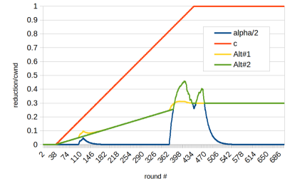
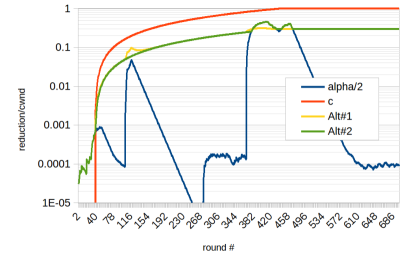
Figure 7: Comparison of Two Alternative CC Behaviour Changeover Algorithms while checking a sweep across the full range of c and extreme values of alpha; linear (left) or log-scale (right)

To quickly check all possible combinations, Figure 7 shows an example time series of alpha with extremely low and high values as it interacts with a sweep of all the values of c, including plateaus at 0 and 1. It shows the CC reduction on a linear and log scale for the two alternative changeover algorithms.

Alt#1 gives the reduction a pro-rata contribution from each of alpha and c, dependent on the value of c. Alt#2 takes the simple maximum of alpha and the value of c scaled down by ALPHA_ABE.

As flow rates scale, the typical value of alpha becomes very small, so it is deceptive to focus on the rounds when alpha is high. Nonetheless, in current networks alpha can approach 100%. With either alternative, when alpha is small, the log plots show that c dominates over most of its range. However, on the left of the log plot it can be seen that alpha dominates when c is close to zero.

Alt#1 behaves more in the spirit of a transition, because it takes pro-rata contributions from each approach. Whereas Alt#2 is more like a binary switch-over. However, the difference is very subtle and unlikely to be noticeable by end-users.

Both alternatives can lead to a reduction greater than APHA_ABE (at about round #400 in Figure 7). This effect is less severe with Alt#1, but it not necessarily a bad thing to reduce cwnd by more than APHA_ABE when congestion is high.

Subsection Summary:

Ultimately, the two alternatives are similar enough that the choice between them can be made on simplicity grounds, in which case Alt#2 is slightly preferable.

6.2 Transition of ECT marking?

When the CC transitions from scalable to classic, should the marking of packets transition from ECT1 to ECT0?

Let us consider a bottleneck with each type of AQM in turn:

Classic AQM:

The only concern here is the sender’s CC behaviour, not its packet markings. If the CC does not transition to classic behaviour, it might outcompete classic flows (if the bottleneck is not FQ). But, it makes no difference whether the sender marks the packets ECT0 or ECT1. Because ’classic’ means RFC 3168, and RFC 3168 requires an AQM to treat ECT0 and ECT1 identically.

L4S AQM:

Here both the packet markings and the CC behaviour need to comply with the L4S spec. [DSBE20] in order to achieve any L4S performance benefit. If packets are not marked ECT1, they will never be classified into an L4S queue.

Therefore, it is not a good idea for an L4S-capable CC to transition packet markings to ECT0, even if it transitions to classic CC behaviour (because it detects a classic ECN bottleneck). It does no harm to anyone by marking its packets ECT1. But if it uses ECT0, then if the bottleneck moves to one that supports L4S [DSBEW20], its packets will be classified into the classic queue and it will never detect the lower delay variability that would trigger its transition back to L4S.

Note that a classic ECN-capable CC does not harm other flows in an L4S queue; it just unnecessarily under-utilizes capacity on its own and competes lamely with L4S flows.

Subsection Summary:

A sender that is L4S-capable should always set its packets to ECT1, irrespective of whether it has transitioned to classic CC behaviour.

7 Evaluation

A large number of evaluation results are available online, with more being added continually. This section gives a brief summary of the results so far. It solely evaluates the passive detection algorithm, and none of the tests yet exercise detection of self-limiting or idling.

7.1 Experimental Conditions

Topology:

Dumbell. Experiments were conducted using 2 pairs of Linux hosts as sender and receiver; the sender in each pair supporting a different congestion control behaviour. The two senders were connected to separate interfaces of a Linux router, with one output interface configured to have various AQMs applied. Then that interface was connected to a bridge, with two ports in turn connected to the two Linux receivers.

Software versions:

All Linux machines (hosts and router) were running a modified Linux kernel v5.4-rc3 [testing/08-04-2020], which included v2.2 of the Classic ECN AQM Fall-back algorithm. Default configuration parameters were used for all software.

Metrics:

Unless otherwise stated for particular experiments, the following metrics were tracked for each Prague flow (per-flow variables were not tracked for ‘background’ Cubic flows):

• classic_ecn score (per RTT), which depends on the 5 metrics below that are not in [brackets];

• Measured RTT, acc_mrtt (per ACK);

• Adaptively smoothed RTT, fbk_srtt (per ACK);

• [For comparison, the pre-existing fixed gain smoothed RTT, srtt (per ACK)];

• Adaptively smoothed mean RTT deviation, fbk_mdev (per ACK);

• Min RTT, rtt_min (per change);

• Slow start threshold, ssthresh (per change);

• [Congestion window, cwnd (per change)];

The following metrics were measured at the AQM for all traffic:

• The throughput per flow, which was sampled per packet each time taking a rolling window of the last 1 s of transmitted data. Throughput was only measured individually for long-running flows; in experiments with short flows, the throughput of all short flows in a class was measured as if they were one aggregate flow; color=olive!40,inline]Bob: Change to rolling sum over 100 ms for 20 s

• The average throughput per flow in each class of flows—scalable or Classic (1 s rolling window, sampled per packet). Short flows were excluded from the average throughput per flow.

• Link utilization (1 s rolling window, sampled per packet);

• Queue delay, measured per packet;

• Drop and marking probability, sampled every 16 base RTTs.

Traffic scenarios:

Simple traffic scenarios with equal RTT long-running flows are used to measure steady-state rate for ‘fairness’ metrics, irrespective of whether such scenarios are typical on the Internet. Scenarios with short flows and a mix of short and long flows are introduced later, including staggered or simultaneous start-up of long-running flows.

7.2 ‘Fairness’ with Long-Running Flows

The two charts in Figure 8 give a high level picture of the improvement in flow rate balance (’fairness’) that the passive Classic ECN AQM detection and fall-back algorithm gives. They show TCP Prague competing with TCP Cubic-ECN over a shared queue CoDel AQM using a $5\times 5$ matrix of different link rates and base RTTs. Each plot (each tall thin cross) shows the $1^{\mathrm{st}}$ percentile, mean and $99^{\mathrm{th}}$ percentile of the normalized rate per flow (see definition below). A value of 1 ($10^{0}$) is the ideal. The left and right-hand charts show the outcome with the algorithm disabled and enabled respectively. In all cases, it can be seen that enabling the algorithm causes TCP Prague to pretty closely balance its flow rate with TCP Cubic-ECN.

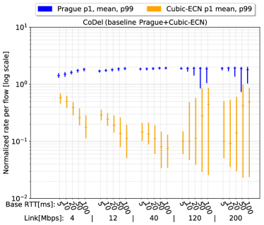
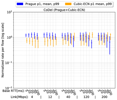
Figure 8: Comparison between Classic ECN AQM Fall-back algorithm when disabled (left) and enabled (right) in TCP Prague over 25 combinations of link-rates and base RTTs. In both cases, the long-running TCP Prague flow competes with a long-running TCP Cubic ECN flow over a CoDel AQM. Normalized rate per flow is defined in the text.

Normalized rate per flow is defined as the ratio of the flow rate, $x$ relative to an ‘ideal’ rate. The ideal rate is defined as the link capacity divided by $n$, where $n$ is the number of flows ($n=2$ in all cases in Figure 8). Thus, normalized rate per flow $=x/(C/n)$. In this ‘fairness’ experiment, rate measurements were taken after allowing flows to stabilize for $T$ s, with $T=5+x*R/100,000$, where $x$ is the flow rate in [b/s] and $R$ is the RTT in [s].

It can be seen that the left-hand chart is similar to Figure 1 in § 1, which we originally used to illustrate the coexistence problem. The link-rates and base RTTs are the same, but in Figure 1 PI2 was used as the Classic AQM and DCTCP was used as the L4S congestion control. In Figure 8 CoDel (not FQ_CoDel) is used as the Classic AQM, because it is likely to be the most difficult single-queue Classic AQM for the algorithm to distinguish from an L4S AQM (see § 3.6 for reasoning).

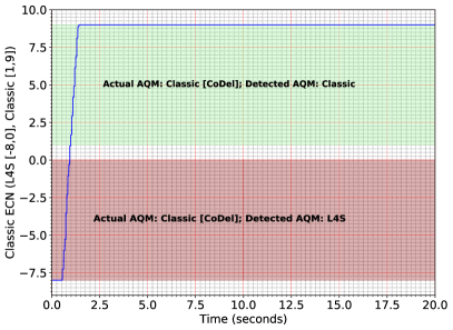
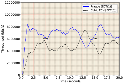
Figure 9: A typical example of the evolution of the classic_ecn score (left) in a long-running TCP Prague flow while competing with 1 long-running Cubic flow in a CoDel AQM bottleneck. The algorithm detects a Classic AQM and switches to classic ABE-Reno behaviour ($\mathtt{classic\_ecn}\geq 1$) after about 1 s. The resulting throughput of each flow is shown on the right [12 Mb/s link; 50 ms base RTT].

In every case, the algorithm rapidly detects a Classic ECN AQM and switches TCP Prague over to its ABE-Reno response to ECN marks, which then competes roughly equally with Cubic. Figure 9 is a typical example time series at 12 Mb/s and 50 ms base RTT. In the left-hand plot, after 0.5 s the classic_ecn variable can be seen starting to move off its -L_STICKY floor (-8) towards classic. It has already fully transitioning to classic (at $\mathtt{classic\_ecn}=1$) after 1 s (about 50 base round trips), then continues onward to $\mathtt{classic\_ecn}=9$ by 1.5 s after the flow started.

The flow throughputs are shown on the right-hand side of Figure 9. The Prague flow (in blue) fills the available capacity after about 1.5 s; at about the same time as its classic_ecn score hits its maximum ‘stickiness’ of 9. Therefore, for the rest of the time, it behaves as ABE-Reno, and competes on roughly equal terms with the Cubic-ECN flow (in black).

7.3 Fairness with Staggered Long-Running Flows

It is necessary to test for cases in which the fall-back algorithm might never see the true minimum RTT. This can occur if one flow starts while a long-running flow is already maintaining a standing queue.

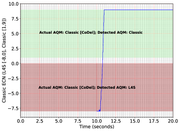
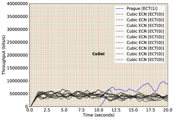
a) c)
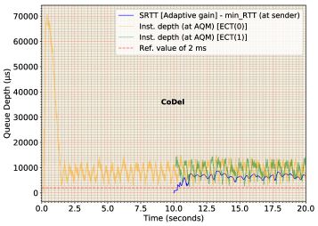
b) d)

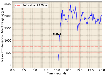
Figure 10: At 10 s a long-running Prague flow joins a standing queue built by 9 Cubic flows over a CoDel AQM. Four variables are tracked: a) classic_ecn score; b) per-flow throughput; c) queue delay (actual (yellow/green) and sender’s estimate (blue)); d) Mean RTT deviation. [40 Mb/s link; 20 ms base RTT]

In the previous section, both flows started simultaneously, whereas Figure 10 shows a case where a single Prague flow joins 9 Cubic-ECN flows after 10 s. It can be seen from Figure 10a) that the Prague flow switches to Classic ABE-Reno behaviour about 0.75 s after it starts. And Figure 10b) shows that the throughput of the Prague flow (blue) competes reasonably ‘fairly’ with the Cubic flows (rate ratio of roughly 1.75).

Thus the fall-back algorithm works despite not correctly measuring the queue delay, as we shall now explain with the aid of Figure 10c), which overlays the queue delay as measured at the AQM (yellow/green) with the smoothed queue delay estimated by the Prague sender’s fall-back algorithm (blue), which uses only end-to-end measurements. It can be seen that Prague’s e2e measurements persistently under-estimate the queue delay by the same amount, which represents its over-estimate of the min RTT, due to only ever having seen a standing queue. Nonetheless, this does not cause the algorithm to switch back to scalable L4S behaviour, for three reasons:

1. The queue delay estimate is not sufficiently incorrect to drop below the queue delay threshold ($\mathtt{D0}=2\,$ms) shown as a a red dashed horizontal);

2. Even if the estimate did drop below the threshold, the algorithm only takes note of queue delay above the threshold, not below (specifically because the min RTT is unreliable);

3. The algorithm also uses RTT variability, and the sender’s instantaneous measurements still lead to a value of mean deviation that is higher than the $750\,\mu$s threshold, as illustrated by the red dashed horizontal in Figure 10d).

7.4 Switching AQM Mid-Flow

Experiments were also conducted to determine the effect of a change in AQM mid-flow. Though unlikely, an AQM change can happen, e.g. if the path of a flow re-routes, or if a different buffer becomes the most bottlenecked on the path. Nonetheless, the purpose of these experiments was more to double-check that the fall-back algorithm does not exhibit any unexpected behaviour during such an event. Nonetheless, it was also interesting to see just how quickly the algorithm could detect such a change.

Figures 11 & 12 show the outcome in one example scenario (40 Mb/s link rate, 10 ms base RTT). The scenarios shown differ only in which AQM was applied first.

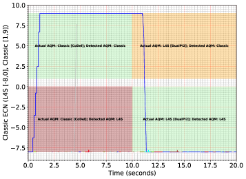
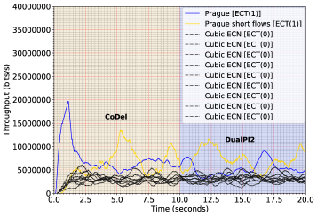
a) c)
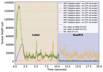
b) d)

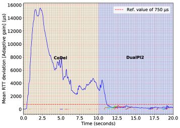
Figure 11: At 10 s the AQM switches from CoDel to DualPI2, while 1 Prague & 9 Cubic-ECN long-running flows proceed. Also a low background load of web-like (type L) Prague flows arrive continually. Four variables are tracked: a) classic_ecn score; b) per-flow throughput; c) queue delay (actual (yellow/green) and sender’s estimate (blue)); d) Mean RTT deviation. [40 Mb/s link; 10 ms base RTT]

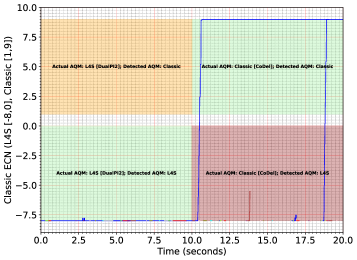
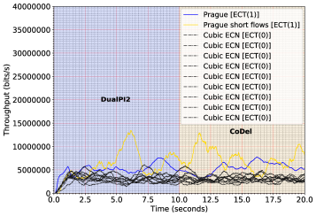
a) c)
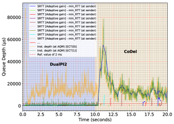
b) d)

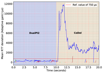
Figure 12: As Figure 11, except the order of the AQM is reversed

The backgrounds of the plots of the classic_ecn scores (Figures 11a) & 12a) have been coloured to show the regions where the score should transition to in green (if the algorithm correctly detects the type of AQM), and where it should transition away from in amber or red. Red represents the unsafe situation where a Prague flow incorrectly detects that the AQM is L4S when it is Classic. Amber represents the safe but incorrect situation where a flow incorrectly detects a Classic AQM when it is L4S. It can be sesen that in both cases, the Prague flow rapidly detects and switches to the correct AQM soon after startup, and again, soon after the switch over.

The evolution of the classic_ecn score in a few of the short Prague flows can be seen starting at their minimum value and rarely moving before the flow finishes (by design). In Figure 12a) a couple of slightly longer short flows can be seen starting to move towards the classic end of the scoring range, but only one (a blue one starting around19 s) lasts long enough to get there.

In both Figures 11b) & 12b) it can be seen that the Prague flow’s throughput seems unperturbed by the switch of AQM. This is because it rapidly detects the type of AQM and its fall-back algorithm quickly adapts between scalable and classic behaviour (or vice versa) as appropriate for the detected AQM.

Incidentally, the yellow plot tracks the total throughput of all short flows (all Prague in this scenario). There is no expectation that their aggregate throughput will relate in any way to the rates of the long-running flows, because short flows act as a semi-unresponsive aggregate.

Figures 11c) & 12c) give a vivid illustration of the difference in the queuing delay that each AQM can achieve. Over the Codel $\rightarrow$ DualPI2 switch, the classic queue induced by the Cubic-ECN traffic stays roughly the same, growing only slightly, as PI2 takes over from CoDel. In contrast, once the Prague flow detects it is in the L4S queue within the coupled DualPI2 AQM structure, its queue rapidly reduces. The chart shows the 2 ms threshold chosen for the algorithm to distinguish between Classic and L4S queues, and it can clearly be seen how the queueing delay of ECT(1) packets (green) and the Prague flow’s estimate of the queueing delay (blue) sit above or below this threshold depending on whether the AQM is respectively Classic or L4S.

Similarly, Figures 11d) & 12d) plot the algorithm’s estimate of the mean deviation of the queue, again clearly showing that the variability of the Classic and L4S AQMs sit respectively above and below the $750\,\mu$s threshold chosen to tell them apart. Incidentally, the small coloured ‘scribbles’ rising from the x-axis are the estimates of mean RTT deviation starting to form in each short flow, up to the point that each one completes.

In summary, the fall-back algorithm clearly detects a changed environment rapidly, and switches fast so that the size of the congestion control’s sawteeth conform to the ’rules’ it expects other flows to be following in each environment. Consequently, there is no discernible change in per-flow throughput across the switch-over, despite the Classic AQM not having any logic for coexistence between Classic and and scalable flows.

7.5 Classic ECN AQM Detection under a Range of Traffic Mixes

The online evaluations already mentioned¹⁰ were used to test the fall-back algorithm in a range of traffic scenarios. Each traffic scenario tests one of the following flow patterns for Prague against another of this same list of flow patterns for Cubic-ECN:

0:

denotes zero flows;

1:

denotes 1 long-running flow;

9:

denotes 9 long-running flow;

L:

denotes a ‘low load’ of synthetic web-like short flows following an exponential arrival process. ‘Low load’ equates to 1 request per second for the 4 Mb/s link rate, scaled up proportionately for high rate links (e.g. 50 req/s for the 200 Mb/s link). A lower load is used as the worst case, because the congestion controls and AQMs cannot settle at any one operating point before the load changes again. Every request opens a new TCP connection, closed by the server after sending data with a size according to a Pareto distribution with $\alpha=0.9$ and minimum and maximum sizes of 1 KB and 1 MB.

1L:

denotes 1 long-running flow combined with load ’L’.

These traffic descriptors are placed either side of a colon to denote each traffic scenario, with the Prague flows always given first. For example, 1:0 denotes 1 long-running Prague flow alone; while 9:L means 9 long-running Prague flows plus a low load of short, web-like Cubic-ECN flows.

This results in a $4\times 5$ matrix of traffic scenarios because, although there are 5 descriptors because there is little point in testing zero Prague flows. Each traffic scenario was then tested in each of the combinations of 5 link rates and 5 base RTTs already seen in Figure 8 Thus each AQM scenario was tested over a matrix of $(4\times 5)\times(5\times 5)=500$ different traffic and environment scenarios. These are clearly far too numerous to include exhaustively in this paper, but the general trend of the results will be described.

Online, there is a ‘traffic light’ visualization of all these experiments.¹⁰ Each experiment was run for 20 s and given a colour in a large matrix of coloured squares depending on the success of Classic ECN AQM detection within that time:

Green

denotes a true positive or true negative, (i.e. correctly detecting the AQM, whether Classic or L4S;

Amber

denotes a false positive, i.e. detecting a Classic AQM when the AQM is actually L4S;

Red

denotes a false negative, i.e. detecting an L4S AQM when the AQM is actually Classic;

False negatives are coloured red because it could be unsafe for TCP Prague to behave as a scalable flow in a Classic AQM, if it is in a shared queue. In such a case, TCP Prague would then outcompete any Classic flows sharing the same bottleneck. In contrast, with false positives, TCP Prague responds to ECN marking with a large classic reduction, potentially under-utilizing the link, but not harming other flows.

Note that, failure of the detection algorithm only leads to the potential for harm not necessarily actual harm. For instance, detection is deemed to have failed if it does not reach the correct state within the 20 s duration of each experiment. And in many experiments the algorithm has to respond to a change after 10 s, leaving it only a further 10 s to succeed. The choice of 20 s and 10 s as deadlines was a subjective trade-off between how long an effect is likely to be noticeable and the impact on the run-time of all the experiments.

Often, given a little longer, the algorithm correctly detects the AQM. Also, detection is deemed to have failed if at least a ‘significant minority’ of short flows switch to Classic behaviour by the time they complete, even though they are over an L4S AQM. All these transient effects are rarely detectable on plots of the resulting flow throughput, let alone detectable to an end-user.

A high level summary of the results so far follows:

• The fall-back algorithm correctly detected a CoDel AQM as Classic in 497 of the 500 scenarios. All three false negatives (0.6% of scenarios) involved zero Cubic-ECN flows, so there were no cases where any Cubic-ECN flow was at risk of being outcompeted by TCP Prague.

• The fall-back algorithm correctly detected that a DualPI2 AQM was L4S in 361 of the 500 scenarios. There were no unsafe false negatives, but the balance of the scenarios (139 or 28%) resulted in a false positive. Of these:

  • 75 (15%) occurred at the 4 Mb/s link rate, because the serialization delay of one packet at that rate is 3 ms, which is greater than the algorithm’s queue depth threshold.

  • 52 (10%) occurred at the 12 Mb/s link rate, for a similar reason, i.e. the threshold queue depth of 2 ms is only two packet serialization delays at this link rate. Detection was correct in a large majority of the single flow tests, but only in a minority of those with multiple simultaneous flows (whether long-running or a mix of long and short).¹²

  • 11 (2%) occurred at the 40Mb/s link rate; more than half (6) occurring with the highest base RTT (100 ms).

  • 1 false positive occurred in the 50 scenarios at link rates above 40 Mb/s.

• Results when the AQM was switched from CoDel to DualPI2 half way through the run (after 10 s) produced similar results to those over DualPI2 alone. However there were more false positives at the largest base RTT of 100 ms, because only introducing the DualPI2 AQM after 10 s left only half as long to detect it and switch to it before the 20 s deadline. Also 2 false negatives crept in. No long-running Cubic flows were present in either of these false-negative cases, so again there was no safety issue.

• When the AQM was switched from DualPI2 to CoDel half way through the run (after 10 s), again the outcome was very similar to that with DualPI2 alone, with false positives in similar types of scenarios. However, this time, more false negatives appeared as well. Again, no long-running Cubic flows were present in any of these false-negative cases with one exception (1:1 at the maximum link rate and base RTT tested).

Failures to detect the correct AQM were typically transient and, as noted earlier, they only indicate the possibility of harm, not actual harm. No discernible effect could be noticed on throughput balance in any of the cases with a false result, whether false positive (amber) or false negative (red). This is evidenced by the throughput results in Figure 8.

In particular, the failures at low link rate typically involved congestion windows that were already close to TCP’s minimum of 2 segments. Therefore it made little difference whether an attempt to reduce cwnd was large or small, because in practice only small reductions were possible.

color=olive!40,inline]Bob: ToDo: Related Work

8 Conclusions

This paper has explained and justified the design of an algorithm that can be used by scalable congestion controls to fall back to Classic (Reno-friendly) behaviour on detection of a Classic ECN AQM. This is intended to ensure that no Classic flow is beaten down by a scalable congestion control such as TCP Prague in any Classic ECN bottlenecks that might be operational on the Internet.

Since the v1 algorithm design, the passive part of the algorithm has been implemented and extensively evaluated over a wide range of link-rates, RTTs and traffic scenarios. This paper now describes v2 of the algorithm. The only change has been to add adaptive smoothing of the RTT EWMAs, and to set or slightly alter the setting of a number of the parameters.

The algorithm has proven itself able to make the Prague congestion control fall back to Classic ABE-Reno behaviour whenever it proves necessary due to a Classic AQM at the bottleneck. The resulting ratio of the throughputs of Prague and Cubic-ECN flows easily falls within the range of about 0.5 to 2. In contrast, without the algorithm, the ratio can be as high as 16.

In no test scenario has the throughput of a Prague flow been persistently greater than twice that of a Cubic-ECN flow. Thus the algorithm satisfies the ‘Prague L4S’ requirement to fall back to Reno-friendly behaviour when operating over a Classic ECN AQM (at least a shared one, and ideally any such AQM). It is therefore a candidate for use as a reference ECN fall-back design in other scalable congestion controls.

Although so far evaluation has only been carried out with CoDel as the Classic AQM, CoDel was chosen as the likely worst-case; being least distinguishable from an L4S AQM. This gives some confidence that planned evaluation with other Classic AQMs will be successful.

9 Future Work

The evaluation in § 7 focuses on the v2 passive detection algorithm based on delay variation in § 3.2. It shows promise. But it gives many false positives at link rates below 12 Mb/s. Also at higher link rates some false positives appear as base RTT exceeds about 80 ms. Initial testing of ideas for further parameter tuning and heuristic adaptation of the thresholds were more promising (see footnotes ^{12 & 13}). So it was originally planned to fully explore these avenues.

Then a large number of tests over a wider range of scenarios was planned, for instance:

• with mixed RTTs, and emulating applications that sometimes self-limit the window;

• over different Classic AQMs that might be deployed in shared queues on the Internet (COBALT, DOCSIS PIE, RED);

• over different L4S AQMs, e.g. FQ_CoDel with a shallow ECN threshold, DualPI2 with a ramp instead of a step;

• with different combinations of TCP Prague features enabled or disabled, e.g. RTT independence, paced chirping;

After all that, it would still be necessary to address the interaction of delay-variation measurements with radio links, and links that add burstiness by aggregating frames.

Therefore, the focus shifted to using discrete metrics rather than delay variation. Design ideas and a feasibility experiment on using the spacing between marks have been written up in § 3.1.5. And an idea called ‘exclusive’ marking for altering the specification of L4S to make it more distinct from Classic ECN marking is written up in § 5.3. Although these approaches still require empirical validation, the range of experiments needed should be far narrower and less onerous.

Since the v2 algorithm was evaluated, there has also been a shift of focus towards out-of-band testing; to validate paths prior to L4S deployment with occasional reviews afterwards. A new section on out-of-band testing has been added at § 4, where a very simple but adequate test is defined. If out-of-band testing is deemed sufficient, nothing more would be necessary than to verify that simple test.

10 Acknowledgements

Transitioning gradually from scalable to classic behaviour, using ECT0 packets for active detection and using the spacing between marks were based on initial ideas suggested by Koen De Schepper. The ideas based on altering the standardization of L4S AQMs (§ 5.3) were suggested by Alex Burr. Thanks are due to Olivier Tilmans and Koen De Schepper for reviewing the design approach and the code, and to Tom Henderson for advice on presentation of the results.

Bob Briscoe was part-funded by the Comcast Innovation Fund. The views expressed here are solely those of the author.

Appendix A Adapting the RTT Smoothing Timescale

Given the EWMA of the RTT is meant to be smoothed over a sawtooth, and it is updated per ACK, naïvely, one would think the smoothing gain should be the reciprocal of the average number of ACKs in a TCP sawtooth, $n_{a}$. However, there are three reasons not to take this naïve approach:

• The whole reason for trying to move away from Classic congestion controls is that the average duration of a sawtooth grows linearly with the congestion window. So, if the smoothing gain tracked $n_{a}$, the classic ECN AQM detection algorithm would become linearly more sluggish as the congestion window scaled up.

• In practice, the duration of a Classic sawtooth does not actually grow linearly as link rate scales, because the longer it takes, the more likely it will mistake some other disturbance for congestion, such as a competing short flow or a bit error.

• Classic ECN AQM detection is only needed for the transition from Classic to scalable (L4S) congestion controls. If the L4S experiment is successful, there will be no need to scale the transition mechanism beyond the flow rates Classic congestion controls can attain today.

Therefore, a formula for the average number of ACKs in a TCP sawtooth $n_{a}$ will be derived, but then the degree by which it scales with congestion window will be reduced using empirical experience, to produce a heuristic that works in practice.

$$n_{a} \approx\mathrm{avg\_packets\_per\_sawtooth}/d$$

$$\approx 1/(p*d),$$ (1)

where $d$ is the delayed ACK ratio (typically 2) and $p$ is the probability of an ECN mark, because a mark ends a sawtooth and on average there will be one mark per $1/p$ packets.

It would be efficient to only recalculate the gains to use for srtt and mdev at the end of every sawtooth, when the slow-start threshold ($S$) is recalculated. We relate $p$ to the average congestion window $W$ using the steady state response function of a Classic congestion control, taking Reno as the worst case [MSMO97]. Then it will be straightforward to relate $W$ and therefore $p$ to $S$.

$$W_{\mathrm{Reno}} \approx\sqrt{\frac{3}{2p}}$$

Substituting for $$p$$ in Equation 1

$$n_{a} \approx 2W_{\mathrm{Reno}}^{2}/3d$$ (2)

For Reno, the average congestion window lies midway between $$S S/\beta \beta$$ and , where is the reduction factor of the congestion control:

$$W_{\mathrm{Reno}} \approx(1+1/\beta)/2*S_{\mathrm{Reno}}$$

Substituting for $$W_{\mathrm{Reno}}$$ in Equation 2

$$n_{a} \approx(1+1/\beta)^{2}/(6d)*S^{2}$$

$$\approx 3/4*S^{2},$$

assuming a typical delayed ACK ratio, $d=2$, and Reno as the worst-case congestion control where $\beta_{\mathrm{Reno}}=0.5$.

For efficiency, the smoothing gain should be an integer power of 2, so that the integer power can be used as a bit-shift. A fast integer base 2 log (such as ilog2()) rounds by truncation. Therefore, for unbiased rounding, $n_{a}$ would need to be scaled up by 3/2 before taking the log. Thus, the integer log of $3/2*3/4*S^{2}\approx S^{2}$ would be taken.

As explained above, in practice an empirical formula for the smoothing gain is used in place of this theoretical formula. Nonetheless, this theoretical number of ACKs per sawtooth helped set an upper bound to the range of formulae to be tried in experiments. The formula for smoothing gain, $g_{\mathrm{fbk_{s}rtt}}$, used in experiments was of the form:

$$g_{\mathrm{srtt}}=U2*S^{U1}.$$

In experiments with a range of link rates between 4 Mb/s and 200 Mb/s and RTTs between 5 ms and 100 ms, the parameters for this formula that resulted in a good compromise between precision and speed of response were:

$$g_{\mathrm{srtt}}=2*S^{3/2}.$$

Currently the mean deviation is smoothed twice as slowly as this, i.e.:

$$g_{\mathrm{mdev}}=g_{\mathrm{srtt}}*2.$$

color=olive!40,inline]Bob: Currently, the Linux code and the pseudocode uses g_mdev = g_srtt * 2

Appendix B Implementation in Integer Arithmetic

B.1 EWMA Precision and Upscaling

The pseudocode below repeats the EWMA pseudocode given in subsection 3.4, but in integer arithmetic including recommended types for the variables and the formulae used to check for overflow. Rationale for the recommended types is given below the pseudocode.

All the variables that are specific to Classic ECN AQM fall-back are prefixed with fbk_, so the EWMAs of srtt and mdev are called fbk_srtt and fbk_mdev.

#define ACC_MRTT_MAX 0xFFFFFFUL    // < 2^24 [us] (=16.7s)
#define FBK_SSTHRESH_MAX 0x0FFF    // < 2^((20 - 2) * 2/3) - 1 = 2^(12)  (see text)
#define FBK_G_DIFF 1               // fbk_g_mdev = fbk_g_srtt * 2^(FBK_G_DIFF)

// Stored variables
u64 fbk_srtt;                // Upscaled smoothed RTT
u64 fbk_mdev;                // Upscaled mean deviation
int fbk_g_srtt_shift;        // srtt gain bit-shift (initialized dependent on ssthresh)
int fbk_g_mdev_shift;        // mdev gain bit-shift (initialized dependent on ssthresh)
u32 fbk_mdev_carry;          // Geometric carry
u32 fbk_depth_carry;         // Geometric carry

// Temporary variables
u32 acc_mrtt;                // Measured RTT from newest unack’d packet
s64 error_;
int delta_shift_;

{   // At start of connection, either after first RTT measurement or from dst cache
    fbk_srtt = acc_mrtt<<fbk_g_srtt_shift;
    fbk_mdev = 1ULL<<fbk_g_mdev_shift; // No need for conservative init, unlike for RTO
}

{   // Per ACK
    acc_mrtt = min(acc_mrtt, ACC_MRTT_MAX);
    // Update EWMAs
    error_ = (u64)acc_mrtt - fbk_srtt>>fbk_g_srtt_shift;
    fbk_srtt += error_;
    fbk_mdev += llabs(error_) - fbk_mdev>>fbk_g_mdev_shift;    // See text re llabs()
}

{   // Per ssthresh change, including when initialized
    delta_shift_ = -fbk_g_srtt_shift;               // Store old shift
    fbk_g_srtt_shift = ilog2(min(ssthresh, FBK_SSTHRESH_SHIFT_MAX));
    fbk_g_srtt_shift += fbk_g_srtt_shift>>1 + 1;    // fbk_g_srtt = 2 * ssthresh^(3/2)
    fbk_g_mdev_shift = fbk_g_srtt_shift + FBK_G_DIFF;   // fbk_g_mdev = fbk_g_srtt * 2

    // Adjust all upscaled variables
    delta_shift_ += fbk_g_srtt_shift;     // Difference between old and new shift
    if (delta_shift_ > 0) {
        fbk_srtt <<= delta_shift_;
        fbk_srtt_carry <<= delta_shift_;
        fbk_mdev <<= delta_shift_;        // Same shift for mdev
        fbk_mdev_carry <<= delta_shift_;
    } else if (delta_shift != 0) {
        delta_shift_ = -delta_shift_;
        fbk_srtt >>= delta_shift_;
        fbk_srtt_carry >>= delta_shift_;
        fbk_mdev >>= delta_shift_;        // Same shift for mdev
        fbk_mdev_carry >>= delta_shift_;
    }
}

The question of the size of the EWMA variables can be broken down into the number range needed prior to upscaling, and the maximum upscaling to be supported.

EWMA Range Prior to Upscaling:

Both the EWMAs (fbk_srtt and fbk_mdev) are fed by the measured RTT acc_mrtt so (prior to upscaling) they never need to hold a value greater than the max usable value of acc_mrtt.

RFC793 defines the maximum segment lifetime (MSL) as 2 minutes (implying a maximum RTT of 4 minutes = $2^{28}\,\mu$s), but it would do no harm if the fall-back algorithm clamped any RTT exceeding, say 15 s to a maximum. A bloated buffer might well lead to an average RTT of a few seconds, but outliers beyond 15 s would unnecessarily pollute the average. If most RTT measurements were this high, there would be little benefit in making classic ECN detection so sluggish. Therefore it will be reasonable to clamp acc_mrtt below $2^{24}\,\mu$s (16.7 s) and use a 32-bit unsigned long integer for it.

Upscaling Limit:

In order to implement an EWMA in integer arithmetic, upscaling the EWMA by the reciprocal $g$ of its gain optimizes the most frequently run parts of the code—those run per ACK. Upscaling by $g$ is straightforward when constant gain is used. But when the gain is adapted (see Appendix A) it is necessary to change the upscaling of the EWMAs, and one or two other variables that depend on this upscaling.

We tried the alternative of always upscaling by a constant maximum factor. This does indeed simplify the calculations needed per sawtooth, but it adds 3 or 4 bit-shifts to the per-ACK calculations. On balance, it was decided to prioritize optimization of per-ACK processing, given the extra per-sawtooth cost is only about half-a-dozen simple operations (a couple of adds; an if; and a few bit-shifts). This involves upscaling by a variable amount that depends on the gain. However, it still leaves the question of what upper bound to fix for upscaling.

A workable upper bound for the number of ACKs over which smoothing is carried out would be $2^{20}$ (a little over 2 minutes at 200 Mb/s assuming 1500 B packets and a delayed ACK every 2 packets). As flow rate scaled beyond this, the adaptation mechanism would stop growing the number of ACKs over which smoothing would occur and the ACK rate would increase, so the maximum smoothing time would reduce, although this might be mitigated somewhat by an increase in the ACK ratio. However, $2^{20}$ is believed to cater for sufficient scale, for the three reasons given in Appendix A (sufficient for transition out of an unscalable regime; the likelihood of disturbance within this time; and ensuring that detection remains responsive).

In the ‘Per ssthresh change’ block of the above pseudocode, when fbk_g_srtt_shift is derived from ssthresh, instead of calculating the unbounded value then clamping it, the intermediate value is clamped to an adjusted down limit before it is raised to the power of 3/2 and doubled. This limit is held in the constant macro FBK_SSTHRESH_SHIFT_MAX, which is reverse engineered as $(20-2)*2/3=12$. This does not limit ssthresh itself. It is just the value of ssthresh at which to cap the number of ACKs over which smoothing is carried out.

Precision and Upscaling Summary:

acc_mrtt uses 23 significant bits, and fbk_g_mdev_shift upscales by a maximum of 19 bits, making 42 bits for the largest EWMA. Therefore the EWMAs will easily fit in a u64, but it will not fit in a u32.

B.2 Iterative Fast Log Calculations with Geometric Carrying

The Classic ECN detection algorithm takes the ratios between the fbk_srtt or fbk_mdev metrics and their reference values and transforms them into linear step changes in the classic_ecn score. This requires a log function but, rather than using floating point arithmetic, it uses the base 2 integer log function ilog2(), which has very low processing cost, but also very little precision. Essentially ilog2() returns the binary order of magnitude of the operand, i.e. the position of the most significant bit that is set to 1 (typically using an assembler instruction such as clz, which stands for count leading zeros).

The order-of-magnitude precision of ilog2() is sometimes good enough, but not always. It is sensitive to whether the configured threshold value is close to a step change in the integer log, which can cause behaviour to stick then suddenly toggle. For instance if the threshold were set to $\mathtt{V0}=500\,\mu$s, in floating point arithmetic $\mathrm{lg}(500)=8.965784285$, but in integer arithmetic $\mathrm{ilog2}(500)=8$. So RTT values lower than the threshold, down to $257\,\mu$s would appear to be at the threshold.

Rather than resort to floating point arithmetic, we implemented an iterative carry algorithm, carry_ilog2(), to accumulate the error and feed it back into the log function, which then outputs the integer values either side of the precise answer, in proportion to the error term at any one time. The cost is 3 adds, 2 bit-shifts and 1 integer multiply. In following pseudocode It is defined at the end and used twice in the ‘Per RTT’ block.

#define PRAGUE_ALPHA_BITSΨ20U  // Upscaling of classic_ecn
#define V_LG 1                 // Weight of queue *V*ariability metric, default 2^(-1)
#define D_LG 1                 // Weight of mean queue *D*epth metric, default 2^(-1)
#define V0_LG_US (10014684UL >> V) // Ref queue *V*ariability [us], default lg(750)<<20
#define D0 2000                    // Ref queue *D*epth [us]
#define D0_LG_US (11498458UL >> D) // Ref queue *D*epth [us], default lg(2000)<<20

// Stored variables
int classic_ecn;               // Classic ECN AQM detection score
u32 rtt_min;                   // Min RTT (uses Kathleen Nichols’s windowed min tracker)

{   // At start of connection, either after first RTT measurement or from dst cache
    fbk_mdev_carry = 1 << fbk_g_mdev_shift;
    fbk_mdev_carry += 1 << (fbk_g_mdev_shift - 1);       // Initialize to 3/2 upscaled
    fbk_depth_carry = 1 << fbk_g_srtt_shift;
    fbk_depth_carry += 1 << (fbk_g_srtt_shift - 1);      // Initialize to 3/2 upscaled
}

{   // Per RTT
    // Temporary variables for readability
    u64 fbk_mdev_;
    u64 fbk_depth_;
    int fbk_mdev_lg_;
    int fbk_depth_lg_;

    fbk_mdev_ = fbk_mdev>>fbk_g_mdev_shift;               // remove upscaling
    fbk_mdev_lg_ = carry_ilog2(fbk_mdev_, fbk_g_mdev_shift, *fbk_mdev_carry)
    // V*lg(v/V0)
    classic_ecn += (u64)fbk_mdev_lg_<<(PRAGUE_ALPHA_BITS - V);
    classic_ecn -=  V0_LG_US;

    fbk_depth_ = fbk_srtt>>fbk_g_srtt_shift - rtt_min;    // Smoothed q depth
    fbk_depth_lg_ = carry_ilog2(fbk_depth_, fbk_g_srtt_shift, *fbk_srtt_carry)
    // D*lg(max(d/D0,1))
    fbk_depth_lg_ <<= PRAGUE_ALPHA_BITS - D
    if (fbk_depth_lg_ > D0_LG_US) {
        classic_ecn += (u64)fbk_depth_lg_ - D0_LG_US;
    }
}

int carry_ilog2(u64 arg, int shift,  u32 *carry) {
    // returns integer base 2 log of arg factored up by carry upscaled by shift
    int arg_lg_;

    // Multiply non-upscaled arg by upscaled geometric carry from previous round
    arg *= *carry;
    arg += 1 << (shift - 1);  // Add upscaled 1/2 to unbias truncation
    arg_lg_ = ilog2(arg) - shift;         // Non-upscaled integer log
    *carry = arg >> arg_lg_;              // Upscaled geometric carry
    return arg_lg_;
}

Being a log function, the carry algorithm needs to be multiplicative (geometric), not additive. The comment ‘Upscaled geometric carry’ tags the line that calculates the carry factor, pointed to by carry, by right bit-shifting the upscaled value of arg by its own integer log.

For instance, if the value of fbk_mdev passed to the algorithm is $500\,\mu$s, $\mathrm{ilog2}(500)=8$, so bit-shifting 500 by 8 is equivalent to $500/2^{8}=1.953125$. Obviously, in integer arithmetic that would always truncate to 1, but by starting with an upscaled value of *carry, an upscaled value of the new carry factor ($1.953125*2^{\mathtt{shift}}$) is produced.

In the next iteration, the next value of fbk_mdev passed to the function as arg is multiplied by the new upscaled carry factor in the line arg *= *carry, which produces an upscaled result. Two lines later, the integer log of this upscaled and factored up value is taken. Continuing the example case with $\mathtt{fbk\_mdev}=500\,\mu$s, the ilog2() function is applied to $500*(1.953125<<\mathtt{shift})$ before shift is subtracted, which produces 9 not 8. As the process iterates, if a steady state of $\mathtt{mdev}=500\,\mu$s were to remain, the output of the integer log would be 8 only 3.422% of the time, while it would be 9 the other 96.578% of the time (thus averaging to $\mathrm{lg}(500)$, which is 8.96578…) .

Even with geometric carry implemented, the average of all the integers logs still understates the value relative to the true floating point log. This is because every right shift to remove the extra degree of upscaling truncates the output. To counteract this truncation bias, 0.5 is added before the downscaling, because 0.5 is the average of all the possible values of the truncated bits. Of course, 0.5 is upscaled by shift before being added, to match the upscaling of the arg that it is added to.

Precision:

When the EWMAs are calculated, fbk_srtt and fbk_mdev are upscaled by their respective $g$ shifts. However, when their logs are taken, copies of these stored upscaled values are taken and reverted to their non-upscaled values. Instead, the carry factor is upscaled by the $g$ shift. Thus, the same number space is needed for upscaling, but the values of the EWMAs need two additional bits on top of their usual maximum size ($<2^{2}4$ as outlined earlier). These two bits consist of:

• The additive adjustment of 0.5 that unbiases the integer log truncation, which consumes one bit in the worst-case.

• The unscaled value of the geometric carry factor, which takes a value between $(1\leq\mathtt{carry}<2)$, which also consumes 1 bit.

Thus, $42+2=44$ bits are needed for the local variable holding the factored up and adjusted EWMA (arg) within the carry_ilog2() function.

B.3 Combining logs

In the passive detection algorithm, both the depth (d) and variability (v) terms involve a log function. So in practice, with judicious choice of the parameters V and D, they could be combined efficiently. For instance, if V=D, then
  V*lg(v/V0) + D*lg(max(d/D0,1))
is equivalent to
  ( d>D0 ? V*lg(v*d/(V0*D0)) : V*lg(v/V0) )

Then the ‘Per RTT’ block of pseudocode above would be replaced with that below, which aggregates two lots of steps into one.

// Stored variables
    fbk_ewmas_carry;        // Replaces fbk_srtt_carry

{   // Per RTT
    // Temporary variables for readability
    u64 fbk_mdev_;
    u64 fbk_depth_;
    u64 fbk_ewmas_;
    int fbk_ewmas_lg_;

    fbk_mdev_ = fbk_mdev>>fbk_g_mdev_shift;             // Remove upscaling
    fbk_depth_ = fbk_srtt>>fbk_g_srtt_shift - rtt_min;  // Smoothed q depth w/o upscaling

    if (fbk_depth_ > D0) {
        fbk_ewmas_ = fbk_mdev_ * fbk_depth_;    // Product of EWMAs
        fbk_ewmas_lg_ = carry_ilog2(fbk_ewmas_, fbk_g_mdev_shift, *fbk_ewmas_carry)
        // V*lg(v*d/(V0*D0)), assuming V = D
        classic_ecn += (u64)fbk_ewmas_lg_<<(PRAGUE_ALPHA_BITS - V);
        classic_ecn -=  V0_LG_US + D0_LG_US;
    } else {
        fbk_mdev_lg_ = carry_ilog2(fbk_mdev_, fbk_g_mdev_shift, *fbk_mdev_carry)
        // V*lg(v/V0)
        classic_ecn += (u64)fbk_mdev_lg_<<(PRAGUE_ALPHA_BITS - V);
        classic_ecn -=  V0_LG_US;
    }
}

Appendix C Algorithm for Filtering Reroutes out of RTT Metrics

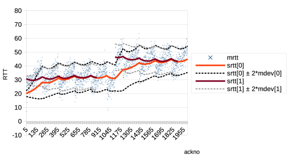
Figure 13: Example plot of ‘incorrect’ (light red) and ‘correct’ (dark red) smoothed RTT and their mean deviations after a reroute at ackno 1100

If the base RTT suddenly changes, e.g. due to a re-route, the smoothed RTT (srtt) could take a long time to converge on the new value. In the meantime, the mean deviation (mdev) will expand, not because there is more queue variability, but because srtt is ‘incorrect’. The resultant increase in mdev could cause the fall-back detection algorithm to incorrectly detect a Classic AQM, even when it is not and there is very littel queue variability.

The pseudocode below is designed to rapidly lock-on to a better smoothed RTT following a significant step change in the base RTT. Consequently, the mean deviation based of this ‘corrected’ smoothed RTT should not increase when there is a step-change in base RTT.

Figure 13 shows an example with both the uncorrected smoothed RTT in bright red (labelled srtt[0]) and the corrected smoothed RTT in dark red (labelled srtt[1]).

Numerous data points for the actual RTT measurements are shown as tiny blue crosses. On closer inspection, a characteristic sawtoothing pattern can be seen in data points as TCP cycles between capacity-seeking and relaxing. At ackno=1100, a step increase in the sawtoothing pattern can be picked out, despite the noisy data. For comparison, the bright red plot labelled srtt[0] is the uncorrected smoothed RTT, which can be seen slowly converging on the new smoothed average after ackno 1100. In contrast, the dark red smoothed RTT labelled srtt[1] rapidly corrects itself by jumping to a ‘better’ value soon after the re-route.

Once the original EWMA converges with the alternative one, the algorithm disables calculation of the alternative to save processing, as can be seen where the dark red plot stops. The algorithm is also useful at the start of a flow, where it can quickly correct an unfortunate initial value of the EWMA, as seen on the left of Figure 13.

The black dashed plots labelled $\mathtt{srtt[0]}\pm 2*\mathtt{mdev[0]}$ illustrate two mean deviations either side of the uncorrected srtt[0] plot. After the re-route, this mean deviation can be seen to expand. In contrast, the grey dashed lines illustrate two mean deviations either side of the corrected srtt[1] plot (labelled $\mathtt{srtt[1]}\pm 2*\mathtt{mdev[1]}$ ). It can be seen that mdev[1] hardly increases at all during the re-route episode.

This is actually a clue to how the algorithm works; whenever there is an outlier, it starts a new EWMA (srtt[1]) from that outlier and initializes the new mean deviation (mdev[1]) with a slightly inflated copy of the original mean deviation (mdev[0]). It only maintains the new EWMA as long as it results in a tighter mean deviation than that based off the original EWMA. The inflation factor for the new mean deviation (K1) is contrived in such a way that the new EWMA will quickly be rejected if it is not ‘better’. In particular, even if the next data point after the outlier is as close as possible to the first outlier without actually being an outlier (with respect to the original EWMA), the alternative EWMA will immediately be disabled (and it will never have been used, because the initial inflated mean deviation was ‘worse’ than the original). The derivation of K1 is left as an exercise for the reader. color=olive!40,inline]Bob: Strictly, a similar exercise using the lower outlier threshold will need to be done, because the outcome of the mean deviation approach is asymmetric. Then the greater value of K1 should be used.

In this way, the algorithm is (usually) able to ignore TCP’s sawtooth jumps, given the mean deviation established over time includes them. By default, outliers are defined as outside $\texttt{K2}=2$ mean deviations.

The pseudocode is given below, followed by a walk-through. It is written as a general-purpose algorithm that could be used to ‘correct’ any EWMAs of RTT and its deviation, whether for Classic ECN AQM detection, retransmit timer calculation or moving averages that are nothing to do with RTT for that matter. Nonetheless, in the case of Classic ECN AQM detection, the variables srtt[] and mdev[] are intended to be equivalent to fbk_srtt and fbk_mdev as defined in pseudocode throughout the rest of this paper (not the srtt and mdev variables already maintained by Linux for RTO calculation). Similarly, for Classic ECN AQM detection, the gain parameters (g_srtt and g_mdev) are intended to be equivalent to fbk_g_srtt and fbk_g_mdev in the rest of this paper.

/* Macros */
#define G1 (1/g_srtt)     // The gain already used to maintain srtt
#define G2 (1/g_mdev)     // The gain already used to maintain mdev
#define K2 2              // Outlier threshold, as multiple of mdev
#define K1 1+G2*(K2*(1-G1)+(K2-1)*(1-G2)-1) // Hysteresis factor (see text later)
// SRTT or MDEV can be used wherever TCP uses srtt or mdev
#define SRTT (srtt[1] && mdev[1] < mdev[0] ? srtt[1] : srtt[0])
#define MDEV (srtt[1] && mdev[1] < mdev[0] ? mdev[1] : mdev[0])

/* Definitions of variables and functions
 *Ψsrtt[1] and mdev[1] are candidate alternatives to srtt[0] and mdev[0],
 *  which are the original uncorrected variables
 */
srtt[2];                 // Array for smoothed RTT (primary and alt)
mdev[2];                 // Array for mean deviation of RTT (primary and alt)
acc_mrtt;                // Latest measured accurate RTT (excl. delayed ACK)
error_;
sign_ = 0;

/* Initialize EWMAs */
srtt[1] = FALSE;        // holds the alt smoothed RTT, but if FALSE disables alt’s.
mrtt[1] = 0;
// srtt[0] and mdev[0] will have been initialized elsewhere (resp. to acc_mrtt and 0)

{ /* Per ACK */
    error_ = acc_mrtt - srtt[0];
    // Check for inlier or outlier on opposite side to the alt srtt
    if (  (abs(error_) <= K2 * mdev[0])                                // Inlier
            ||  (srtt[1] && (sign_ * error_ <= K2 * mdev[0])) ) {      // Opp. outlier
        if (srtt[1]) {
            mdev[1] += G2 * (abs(acc_mrtt - srtt[1]) - mdev[1])); // Update alt mdev
            if (mdev[1] > mdev[0])) {    // suppress alt’s if worse mean deviation
                srtt[1] = FALSE;
            } else {                     // Continue to maintain alt srtt
                srtt[1] += G1 * (acc_mrtt - srtt[1]);
            }
        }
    } else {                             // Outlier (on same side if alt srtt enabled)
        if (srtt[1]) {                   // Continue to maintain alt srtt
            mdev[1] += G2 * (abs(acc_mrtt - srtt[1]) - mdev[1]));
            srtt[1] += G1 * (acc_mrtt - srtt[1]);
        } else {                         // Initialize alt’s
            mdev[1] = mdev[0] * K1;      // Inflate by K1 for hysteresis
            srtt[1] = acc_mrtt;
            sign_ = sgn(error_);         // Record which side the outlier is on
        }
    }

    // Regular update of non-alt srtt and mdev  (order-significant)
    mdev[0] += G2 * (abs(acc_mrtt - srtt[0]) - mdev[0]));
    srtt[0] += G1 * (acc_mrtt - srtt[0]);
}

Pseudocode Walk-Through

The purpose of each variable is assumed to be self-explanatory from the comments in the pseudocode. So this explanation will focus on the logic, which all executes on a per-ACK basis.

The structure of the main ‘if’ block consists of two inter-locked conditions in a bistable flip-flop arrangement:

• Whether the latest RTT is an outlier with respect to srtt[0] (and, whether it outlies on the same side as the alternative EWMA, if one is enabled);

• Whether alternative EWMAs are enabled (i.e. whether srtt[1] is non-zero).

Within each branch of the “outlier?” condition, there is an “alt’s enabled?” condition, so the code flip-flops as follows:

• If “outlier?” is true, and “alt’s enabled?” is not, alt’s are enabled.

• If “outlier?” is false, and “alt’s enabled?” is true, then alt’s are tested to see if they should be disabled (they are disabled if the alternative mdev[1] is worse (larger) than the original mdev[0]).

In the stable state when alternative EWMAs are enabled, they are maintained as normal. And in the stable state when alternative EWMAs are disabled, they are not. This prevents the code doing unnecessary per-ACK work. In production code, a tolerance could easily be added to disable maintenance of alternative EWMAs sooner; when they are hardly any better than the originals.

Once the main ‘if’ block completes, the original EWMAs are updated, as always.

The macros SRTT and MDEV are provided for other code to use. They compare the mean deviation of the two EWMAs and use the best (smallest). In production code, to make these macros more efficient, when srtt[1] is set to FALSE to disable alternative EWMAs, mdev[1] could be set to a special ‘inifinite’ value, so that these macros would not need to test srtt[1] as well as mdev[1].

Appendix D Core or Peering Link with Shared-Queue Classic ECN AQM

First, for brevity, we will use the term ‘common link’ for either a core link or a peering link. This appendix is about the possibility that such a common link could use a shared-queue Classic ECN AQM, and that it could become a bottleneck.

Initially, let us assume an ideal situation in which end systems all ensure equal flow rates at a bottleneck and let us define the equal division of a bottleneck’s capacity among all flows bottlenecked there as the ’equitable rate’ for that bottleneck.

Usually networks are designed so that flows bottleneck in access links. If the number of flows converging into a common link grows, even though they are all bottlenecked elsewhere, there will come a point where the sum of all the flows feeding traffic into the common link exceeds its capacity. If the number of flows continues to rise, the equitable rate for the common bottleneck will continue to reduce. As the equitable rate reduces below the highest capacity access links, the bottleneck for any lone flow in each of those access links will move to the common link.

Let us now imagine that the equitable rate has just reduced to 50% of the capacity of the fastest access link feeding the common bottleneck. If it contains one flow, that will now be running at half the access rate. If it contains two flows, the bottleneck for them will start to move to the common link as well.

Now let’s change the scenario by replacing some classic sources with L4S. At the common bottleneck (still assuming a Classic ECN AQM), there will be little variability in the queue because of the high degree of multiplexing. So as the bottleneck moves there, L4S flows will not detect a classic ECN bottleneck and they will yield less than any classic flows. Classic flows will end up below the equitable rate and L4S flows above it. However, as L4S flows increase, they will bottleneck in their own access link again, which will naturally limit the inequality to $100\%/50\%=2\times$.

Of course, serious anomalies might concentrate so much load at a common link that the equitable rate reduces to less than 50% of the fastest access, say $x\%$. Then the worst inequality would be $100/x\times$. But it is extremely rare for an anomaly to even reduce $x$ to 50%. In robustly designed networks, even during an anomaly, $x$ will only just dip below 100%, e.g. 95%. Then the worst inequality due to classic ECN fall-back not detecting a classic ECN AQM in a highly multiplexed common link would be $100/95=1.05\times$.

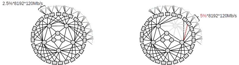
Figure 14: Example before (left) and after (right) a dual anomaly that shifts congestion to a core link

Example:

Starting with the network as designed on the left of Figure 14, the 8 circles in the centre are core routers. The rectangles connected around them are broadband network gateways (BNGs), each dual-homed to two core routers, and each providing Internet access to 8192 customer access links. For ease of explanation, the access links all have the same 120 Mb/s capacity.

The network is designed on the assumption of 2.5% access network utilization outwards, i.e. 2.5% of access links are fully utilized at any one time (or proportionately more than 2.5% are partially utilized). Thus, each BNG needs 2.5%*8192*120 Mb/s = 25 Gb/s. The core links are 40 Gb/s. Assuming reasonably equal load balancing in the core (e.g. randomized equal cost multipath routing), this implies each core link is designed to be utilized at roughly $25/(40*2)=31\%$.

The core’s design utilization is under 50%, which is common for dual-homed cores because, if one core router or link fails, the remaining core capacity will still be sufficient. This keeps the BNGs as the bottlenecks (then more costly per-customer schedulers only need to be deployed at one node on each path).

Now let’s consider two anomalies at once, as on the right hand side of Figure 14. As well as a core node failure, there happens to be unusually high utilization on one BNG, averaging 5%; double the design utilization. This BNG needs 50 Gb/s of core capacity, but it only has one 40 Gb/s link left to connect it to the core. This moves the bottleneck from the BNG to the interface from the core router into the core link shown coloured red. However core routers do not provide per-customer scheduling, so the capacity share that each customer gets now depends on their end-system congestion control algorithms (e.g. TCP), not the network’s schedulers.

If every one of the 5% of customers actively downloading at any one time were using just a single Classic flow with perfect capacity sharing, each access link would be utilized at $40\,Gb/s/(5\%*8192)/120\,Mb/s=81\%$. Therefore, if one customer was to switch to an L4S congestion control instead of Classic, as soon as it used more than $1/0.81=1.23\times$ the Classic equitable share, its bottleneck would shift back to its own access link, thus limiting any further advantage.

This would be no different from the similar common link bottleneck scenario where all customers except one open a single flow. The one opening more flows can only get $1.23\times$ more capacity than everyone else before their bottleneck shifts back to their own access link.

In summary:

Generally, public Internet access networks do not rely on end-system congestion controls to equitably share out capacity between their customers. They rely on per-customer schedulers, but they usually only deploy these at one node on the path, which they design to be the bottleneck. A core or peering link can become the bottleneck under anomalous conditions, so that capacity sharing does temporarily rely on end-system congestion controls. However, if it does, any individual congestion control only has limited scope to take advantage of the situation before it becomes bottlenecked again within its own access link.

Document history

Version	Date	Author	Details of change
00A	20 Oct 2019	Bob Briscoe	First draft.
00B	21 Oct 2019	Bob Briscoe	Moved alt-srtt algo to appendix and made optional, also corrected K1 and used MDEV_MAX. Completed all the discussions about other factors. Just the pseudocode to pull it all together left to do.
00C	23 Oct 2019	Bob Briscoe	First full draft. Completed pseudocode that pulls all the metrics together.
00D	02 Nov 2019	Bob Briscoe	Added active detection section. Other minor alterations.
01	02 Nov 2019	Bob Briscoe	Issued as a complete design, but still some corners to investigate.
01A	02 Nov 2019	Bob Briscoe	Evaluation section ToDo.
01B	06-Mar-2020	Bob Briscoe	Corrected re-route pseudocode
01C	25-Mar-2020	Bob Briscoe	Incorporated improvements from testing & evaluation
01D	05-Apr-2020	Bob Briscoe	Added appendices on Adaptive RTT Smoothing & Implementation; Re-wrote appendix on Reroutes and added example to appendix on core links.
01E	15 Apr 2020	Bob Briscoe	Passive Algorithm v2; Added Asad as co-author, Rewrote Problem Statement; Subdivided Passive Detection section; Added Adaptive Smoothing subsection; Rewrote Parameters subsection; Added Evaluation section; Improved throughout.
01F	18 Apr 2020	Bob Briscoe	Improved clarity & correctness of Eval section and added switching of AQM subsection. Added Conclusions and Further Work.
02	18 Apr 2020	Bob Briscoe	Editorial corrections, mainly in Eval section.
02A	19 Apr 2020	Bob Briscoe	Adding more todo notes; editorial corrections.
02B	16 Feb 2021	Bob Briscoe	Updated link to online evaluation results.
02C	17 Feb 2021	Bob Briscoe	Restructured to add sections with new ideas. Added section on spacing between marks (§ 3.1.5).
03	19 Feb 2021	Bob Briscoe	Completed new ideas sections on: exclusive marking (§ 5.3) and out-of-band testing (§ 4). Altered top and tail sections appropriately to accommodate.

References

- [A+10] Mohammad Alizadeh et al. Data Center TCP (DCTCP). Proc. ACM SIGCOMM’10, Computer Communication Review, 40(4):63–74, October 2010.
- [AKM04] Guido Appenzeller, Isaac Keslassy, and Nick McKeown. Sizing Router Buffers. Proc. ACM SIGCOMM’04, Computer Communication Review, 34(4), September 2004.
- [APB09] M. Allman, V. Paxson, and E. Blanton. TCP Congestion Control. Request for Comments 5681, RFC Editor, September 2009.
- [APS99] M. Allman, V. Paxson, and W. Stevens. TCP Congestion Control. Request for Comments 2581, RFC Editor, April 1999.
- [BCC+15] Wei Bai, Li Chen, Kai Chen, Dongsu Han, Chen Tian, and Hao Wang. Information-Agnostic Flow Scheduling for Commodity Data Centers. In 12th USENIX Symposium on Networked Systems Design and Implementation (NSDI 15), pages 455–468, Oakland, CA, 2015. USENIX Association.
- [BEDSBW20] Bob Briscoe (Ed.), Koen De Schepper, Marcelo Bagnulo, and Greg White. Low Latency, Low Loss, Scalable Throughput (L4S) Internet Service: Architecture. Internet Draft draft-ietf-tsvwg-l4s-arch-06, Internet Engineering Task Force, March 2020. (Work in Progress).
- [Bra89] R. Braden. Requirements for Internet Hosts – Communication Layers. Request for Comments 1122, RFC Editor, October 1989.
- [Bri15] Bob Briscoe. Review: Proportional Integral controller Enhanced (PIE) Active Queue Management (AQM). Technical Report TR-TUB8-2015-001, BT, May 2015.
- [Bri19] Bob Briscoe. Per-Flow Scheduling and the End-to-End Argument. Discussion Paper TR-BB-2019-001, bobbriscoe.net, July 2019.
- [DOC19] Data-Over-Cable Service Interface Specifications DOCSIS® 3.1; MAC and Upper Layer Protocols Interface Specification. Specification CM-SP-MULPIv3.1-I17-190121, CableLabs, January 2019.
- [DSBE20] Koen De Schepper and Bob Briscoe (Ed.). Identifying Modified Explicit Congestion Notification (ECN) Semantics for Ultra-Low Queuing Delay (L4S). Internet Draft draft-ietf-tsvwg-ecn-l4s-id-10, Internet Engineering Task Force, March 2020. (Work in Progress).
- [DSBEW20] Koen De Schepper, Bob Briscoe (Ed.), and Greg White. DualQ Coupled AQM for Low Latency, Low Loss and Scalable Throughput (L4S). Internet Draft draft-ietf-tsvwg-aqm-dualq-coupled-11, Internet Engineering Task Force, March 2020. (Work in Progress).
- [FJ93] Sally Floyd and Van Jacobson. Random Early Detection Gateways for Congestion Avoidance. IEEE/ACM Transactions on Networking, 1(4):397–413, August 1993.
- [Flo03] Sally Floyd. HighSpeed TCP for Large Congestion Windows. Request for Comments 3649, RFC Editor, December 2003.
- [GM02] Liang Guo and Ibrahim Matta. Scheduling Flows with Unknown Sizes: Approximate Analysis. SIGMETRICS Perform. Eval. Rev., 30(1):276–277, June 2002.
- [HJMT+18] T. Hoeiland-Joergensen, P. McKenney, D. Täht, J. Gettys, and E. Dumazet. The FlowQueue-CoDel Packet Scheduler and Active Queue Management Algorithm. Request for Comments RFC8290, RFC Editor, January 2018.
- [HRX08] Sangtae Ha, Injong Rhee, and Lisong Xu. CUBIC: a new TCP-friendly high-speed TCP variant. SIGOPS Operating Systems Review, 42(5):64–74, July 2008.
- [Jac88] Van Jacobson. Congestion Avoidance and Control. Proc. ACM SIGCOMM’88 Symposium, Computer Communication Review, 18(4):314–329, August 1988.
- [JK88] Van Jacobson and Michael J. Karels. Congestion Avoidance and Control. Technical report, Laurence Berkeley Labs, November 1988. (a slightly modified version of the original published at SIGCOMM in Aug’88 [Jac88]).
- [KWAF18] Naeem Khademi, Michael Welzl, Grenville Armitage, and Gorry Fairhurst. TCP Alternative Backoff with ECN (ABE). Request for Comments RFC8511, RFC Editor, December 2018.
- [MSMO97] Matthew Mathis, Jeffrey Semke, Jamshid Mahdavi, and Teunis Ott. The Macroscopic Behavior of the TCP Congestion Avoidance Algorithms. SIGCOMM Comput. Commun. Rev., 27(3):67–82, 1997.
- [MSSM12] G. R. Moktan, S. Siikavirta, M. Särelä, and J. Manner. Favoring the short. In Proc. IEEE INFOCOM Workshops, pages 31–36, March 2012.
- [NJ18] Kathleen Nichols and Van Jacobson. Controlled Delay Active Queue Management. Request for Comments RFC8289, RFC Editor, January 2018.
- [PGI+19] J. Palmei, S. Gupta, P. Imputato, J. Morton, M. P. Tahiliani, S. Avallone, and D. Täht. Design and Evaluation of COBALT Queue Discipline. In 2019 IEEE International Symposium on Local and Metropolitan Area Networks (LANMAN), pages 1–6, 2019.
- [PPP+13] Rong Pan, Preethi Natarajan Chiara Piglione, Mythili Prabhu, Vijay Subramanian, Fred Baker, and Bill Ver Steeg. PIE: A Lightweight Control Scheme To Address the Bufferbloat Problem. In High Performance Switching and Routing (HPSR’13). IEEE, 2013.
- [RFB01] K. K. Ramakrishnan, Sally Floyd, and David Black. The Addition of Explicit Congestion Notification (ECN) to IP. Request for Comments 3168, RFC Editor, September 2001.
- [Sd02] Shanchieh Yang and G. de Veciana. Size-based adaptive bandwidth allocation: optimizing the average QoS for elastic flows. In Proc. IEEE Conference on Computer Communications, volume 2, pages 657–666, June 2002.
- [WP17] Greg White and Rong Pan. Active Queue Management (AQM) Based on Proportional Integral Controller Enhanced (PIE) for Data-Over-Cable Service Interface Specifications (DOCSIS) Cable Modems. Request for Comments RFC 8034, RFC Editor, February 2017.
- [ZTH04] Thomas Ziegler, Hung Tuan Tran, and Eduard Hasenleithner. Improving Perceived Web Performance by Size Based Congestion Control. In Proc 3rd Int’l IFIP-TC6 Networking Conf., page 687, May 2004.