Precision measurements of the gradient of the Casimir force between ultra clean metallic surfaces at larger separations

Abstract

We report precision measurements of the Casimir interaction at larger separation distances between the Au-coated surfaces of a sphere and a plate in ultrahigh vacuum using a much softer cantilever of the dynamic atomic force microscope-based setup and two-step cleaning procedure of the vacuum chamber and test body surfaces by means of UV light and Ar-ion bombardment. Compared to the previously performed experiment, two more measurement sets for the gradient of the Casimir force are provided which confirmed and slightly improved the results. Next, additional measurements have been performed with a factor of two larger oscillation amplitude of the cantilever. This allowed obtaining meaningful results at much larger separation distances. The comparison of the measurement data with theoretical predictions of the Lifshitz theory using the dissipative Drude model to describe the response of Au to the low-frequency electromagnetic field fluctuations shows that this theoretical approach is experimentally excluded over the distances from 250 to 1100 nm (i.e., a major step forward has been made as compared to the previous work where it was excluded up to only 820 nm). The theoretical approach using the dissipationless plasma model at low frequencies is shown to be consistent with the data over the entire measurement range from 250 to 1300 nm. The possibilities to explain these puzzling results are discussed.

I Introduction

Extensive studies of the Casimir force in the last two decades lead us to conclude that this fluctuation-induced quantum phenomenon is of considerable importance for both fundamental physics and its technological applications (see the monograph 1 and reviews 2 ; 3 ; 4 ). For almost half a century it was generally believed that the Lifshitz theory 5 provides quite a satisfactory description of the van der Waals and Casimir forces acting between the closely spaced surfaces made of various materials. In so doing the single input parameter needed to make theoretical predictions was the frequency-dependent dielectric permittivity of the interacting bodies describing their response to the electromagnetic field. Contrary to expectations, several precise measurements performed in the last fifteen years resulted in contradictions between experiment and theory which are sometimes called the Casimir puzzle and Casimir conundrum to specify the problems arising for metallic and dielectric or semiconductor materials, respectively 5a ; 5b .

The Casimir puzzle consists in the fact that theoretical predictions of the Lifshitz theory for metallic test bodies obtained with inclusion of the relaxation properties of conduction electrons are excluded by the measurement data of all precise experiments at short separations 6 ; 7 ; 8 ; 9 ; 10 ; 11 ; 12 ; 13 ; 14 ; 15 . The dielectric response of metals used in computations is found from the optical data extrapolated down to zero frequency by means of the Drude model, where the relaxation parameter $\gamma$ describes the energy losses of conduction electrons. It is puzzling also that if one puts $\gamma$ equal to zero (as if there were no energy losses at low frequencies) the Lifshitz theory comes to good agreement with the measurement data of the same experiments 6 ; 7 ; 8 ; 9 ; 10 ; 11 ; 12 ; 13 ; 14 ; 15 (recall that all of them have been performed at separations below 750 nm between the interacting bodies). This means that the dissipationless plasma model, which is in fact applicable only at high frequencies in the region of infrared optics, works well for some reasons even at low frequencies characteristic of the normal skin effect. The problem is aggravated by the fact that for metals with perfect crystal lattices the Casimir entropy calculated within the Lifshitz theory using the Drude model violates the Nernst heat theorem although the same satisfies it if the plasma model is used 16 ; 17 ; 18 ; 19 ; 20 ; 21 .

In a similar way, the term Casimir conundrum is applied in reference to the fact that theoretical predictions of the Lifshitz theory for dielectrics and dielectric-type semiconductors obtained with the inclusion of the dc conductivity are excluded by the measurement data of several experiments 23 ; 24 ; 25 ; 26 ; 27 . If the conductivity of dielectric materials at room temperature is disregarded, the Lifshitz theory comes to agreement with the same data 22 ; 23 ; 24 ; 25 ; 26 ; 27 . By analogy with the case of metals, it has been proven that the Casimir entropy calculated in the framework of the Lifshitz theory violates the Nernst heat theorem if the conductivity of dielectrics is taken into account which is otherwise satisfied 28 ; 29 ; 30 . Considering that all dielectric materials possess a rather small but nonzero electric conductivity at any nonzero temperature, the situation should be considered as paradoxical.

Resolution of the problems arising in the Lifshitz theory for both metallic and dielectric materials is of major importance for applications of the Casimir force in nanotechnology. With the decrease in separations between the moving parts of microelectromechanical devices below a micrometer, the Casimir force becomes dominant. Because of this, it has long been proposed 31 that the next generation of micro- and nanodevices will exploit the Casimir force for their functionality. In the early twenty first century, extensive studies of the role of Casimir force in microdevices have been conducted and a lot of devices driven by the Casimir force, such as oscillators, switches, microchips etc., have been proposed 32 ; 33 ; 34 ; 35 ; 36 ; 37 ; 38 ; 39 ; 40 ; 41 ; 42 ; 43 ; 44 ; 45 ; 46 . The description of their functionality on the basis of the Lifshitz theory essentially depends on whether the dissipative Drude or the dissipationless plasma model is used in extrapolation of the optical data to low frequencies. This places strong emphasis on the Casimir puzzle and Casimir conundrum as they impact fundamental physics as well as technology.

All precision measurements of the Casimir interaction mentioned above lead to meaningful results at relatively short separations below 750 nm between the test bodies (with the single exception of measuring the Casimir-Polder force 22 relevant to the Casimir conundrum). After the experiment 14 on measuring the difference Casimir force was performed, where the theoretical predictions of the Lifshitz theory using the Drude and plasma models differ by up to a factor of 1000, an exclusion of the former within this separation range was conclusively established. In so doing the role of different background effects, such as the surface roughness 47 ; 48 , variations in the optical data 49 , patch potentials 50 ; 51 etc., as well as the validity of calculation procedure (including the role of deviations from the proximity force approximation 53a ; 52 ; 53 ; 54 ; 55 ), were investigated in detail.

Special attention was paid to the background forces due to patch potentials which become much larger than the Casimir force at separations of a few micrometers. Thus, in Ref. 56 an attempt was undertaken to extract the Casimir force from up to an order of magnitude larger forces between a centimeter-size spherical lens and a plate, presumably caused by the patch potentials, by means of some fitting procedure. The obtained Casimir force was found to be in better agreement with the Drude model approach. It was shown 57 , however, that depending on uncontrolled imperfections on the lens surface the obtained results may agree with equal ease either with the Drude or the plasma model approaches.

Taking into account the significance of the above problems in Casimir physics, which remain unsolved for almost twenty years, in Ref. 58 an upgraded atomic force microscope (AFM)-based technique was developed and an advanced surface cleaning procedure was used in order to eliminate the role of patch potentials and make progress towards a precision measurement of the Casimir interaction at larger separations. For this purpose both interior surfaces of the vacuum chamber and Au-coated test bodies (the sphere and the plate) were successively cleaned by means of UV light and Ar ions. Another improvement was the use of a much softer cantilever. These allowed the separation-independent and low residual potential difference as well as a sixfold decrease of the systematic error in measuring the gradient of the Casimir force. The measurement data have been compared with theoretical predictions of the Lifshitz theory obtained using the extrapolations of the optical data of Au to zero frequency by means of the Drude and plasma models. As a result, the Drude model approach was excluded and the plasma model approach confirmed by the data up to the sphere-plate separation distance of 820 nm.

In this paper, we continue the investigation of the Casimir force between an Au-coated sphere and a plate at larger separation distances using an upgraded technique and the cleaning procedure of Ref. 58 . The results reported in the rapid communication 58 were based on a single measurement set (the gradient of the Casimir force was measured for 21 times at each separation over the range from 250 to 950 nm with a step of 1 nm). Here, we discuss the data of two additional measurement sets and present the mean results from all the three sets. The comparison of these results with theoretical predictions of the Lifshitz theory made using two different statistical procedures leads to the exclusion of the Drude model approach and confirmation of the plasma model approach up to the separation of 850 nm.

Next we present additional measurements with increased oscillation amplitude of the cantilever (20 nm instead of 10 nm in Ref. 58 ) which decreased by the factor of 1.375 the systematic error in measuring the frequency shift. The obtained measurement data are again compared with theoretical predictions of the Lifshitz theory using the two alternative statistical approaches. As a result, the Drude model approach is excluded up to much larger separation distance of 1100 nm. The plasma model approach is found to be consistent with the data up to the separation of $1.3~{}\mu$m. The importance and possibilities to test the Lifshitz theory experimentally at even larger separations are discussed.

The paper is organized as follows. In Sec. II we briefly present the upgraded AFM-based setup and some additional details of the cleaning procedure by means of UV light and Ai-ion bombardment. Section III is devoted to the measurement results with relatively small oscillation amplitude of the cantilever and their comparison with theory. In Sec. IV the measurement results at larger separations are presented and compared with theoretical predictions. In Sec. V the reader will find our conclusions and a discussion of future prospects.

II Upgraded setup with a two-step surface cleaning

We have measured the gradient of the Casimir force between an Au-coated hollow glass sphere and an Au-coated polished Si wafer by means of the AFM-based setup working in the frequency-shift mode in ultrahigh vacuum. The main steps in making these measurements are the following.

The force-sensitive element in our setup shown schematically in Fig. 1 is a rectangular cantilever. As compared to previous experiments 10 ; 11 ; 12 ; 13 ; 15 , the precision of force measurements here was improved by increasing the sensitivity of the cantilever through a decrease of its spring constant. The cantilever spring constant is given by 59

$$k=\frac{wv^{3}Y}{4L^{3}},$$ (1)

where $w,~{}v$, and $L$ are the width, thickness, and length of the cantilever beam, respectively, and $Y$ is its Young’s modulus. As is seen from Eq. (1), the spring constant can be effectively decreased by reducing the thickness of the beam.

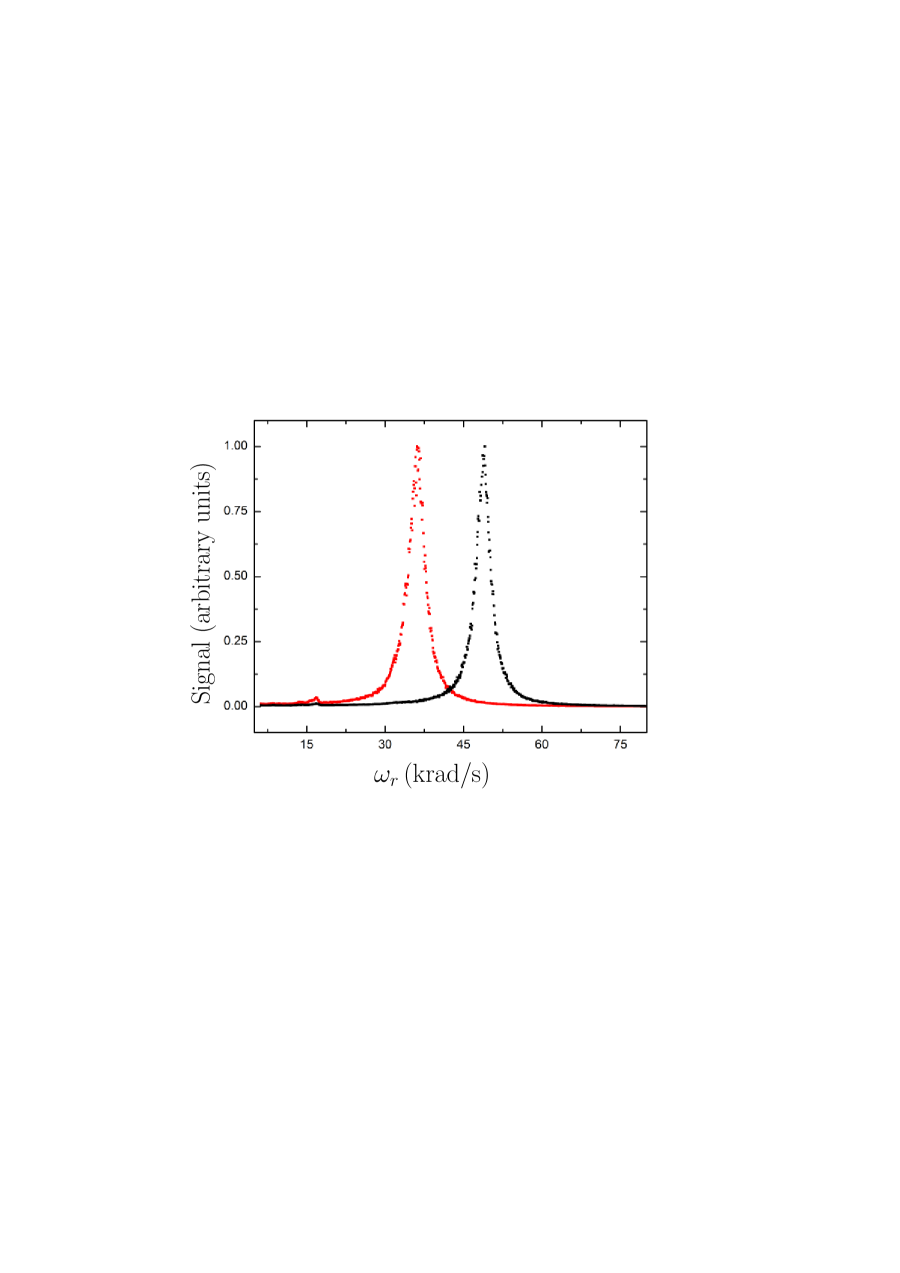
Figure 2: The cantilever thermal noise oscillation spectrum is shown as a function of frequency before (right peak) and after (left peak) etching.

This was achieved by means of the etching process. At first, the cantilever was rinsed with buffered HF solution (BOE 6:1) for 1 min. followed by DI water to remove the oxide layer. Then the cantilever was etched with 60% KOH solution at $T=50\,{}^{\circ}$C for 55 s. Mild agitation by hand was used to obtain a uniform etching. Relatively high concentration of KOH solution and high temperature were necessary to achieve sufficiently smooth surfaces after etching 61 . The spring constant was measured using the thermal oscillation spectrum of the cantilever, as discussed in Ref. 60 , both before and after the etching process and the values $k=0.013$ and 0.0063 N/m were obtained, respectively. As a result, the resonant frequency of the cantilever $\omega_{0}$ was reduced from its original value $4.877\times 10^{4}~{}$rad/s to $3.608\times 10^{4}~{}$rad/s (see Fig. 2). These measurements were made in ambient conditions at room temperature.

The first test body of our setup is the hollow glass sphere of approximately $43~{}\mu$m radius. It was made from liquid phase which leads to almost perfectly spherical shape with less than 0.1% relative difference along any two perpendicular axes. The sphere was baked at $60\,{}^{\circ}$C for two hours to remove volatile components. Then it was picked up using a bare optical fiber and attached to a cantilever using a very small amount of conducting silver epoxy (see Fig. 1). The process of attachment was performed under an optical microscope.

Following the attachment of the sphere, the Au coating was applied on the cantilever and the sphere using an E-beam evaporator at a pressure $5\times 10^{-6}~{}\mbox{Torr}\approx 0.7\times 10^{-3}~{}$Pa. In contrast to thermal evaporators used in previous experiments, the E-beam evaporator leads to smoother surfaces and lower roughness. The Au coating speed was 2 Å/s and the thickness of the Au layer was $118\pm 1~{}$nm. After the measurements of the Casimir force were completed, the radius of the Au-coated sphere was measured to be $R=43.466\pm 0.042~{}\mu$m using a calibrated scanning electron microscope and software ImageJ to precisely determine the sphere boundary. Quantification of the deviation from a perfect sphere was done by finding the difference between the maximum and minimum diameters for any two perpendicular line scans of the sphere diameter in ImageJ. The respective difference in the sphere radii was taken into account in the total error of $R$ indicated above. As a result, the error in determination of the sphere radius was decreased as compared to previously reported in the literature (see, e.g., Refs. 10 ; 60a ; 60b ). The rms roughness on the sphere surface $\delta_{s}=1.13~{}$nm was also measured when the work was completed. After the Au coating, the spring constant of a cantilever with sphere attached increased to $k=0.007353$ N/m, and its resonant frequency decreased to $\omega_{0}=0.9444\times 10^{4}~{}$rad/s in ultrahigh vacuum.

The Au-coated sphere-cantilever system was attached to two block piezoelectric actuators. The cantilever is electrically grounded (see Fig. 1). The cantilever motion was monitored using a fiber optical interferometer with a laser light wavelength of 1550 nm. For so doing, single mode 1550 nm fibers were used. To improve the finesse of the Fabry-Perot cavity of the interferometer, the reflectance of the top side of the cantilever was increased with a layer of Au of 40 nm thickness.

The second test body of our setup is a polished Si wafer of $1\times 1~{}\mbox{cm}^{2}$ area and of $500~{}\mu$m thickness used as a plate. It can be considered infinitely large as compared to the sphere (in Fig. 1 the test bodies are not shown to scale). The Si wafer was HF washed and then coated with $120\pm 1~{}$nm of Au using an E-beam evaporator. This resulted in the rms roughness $\delta_{p}=1.08~{}$nm measured after finishing the Casimir force measurements. The plate was mounted on a piezoelectric tube which is used to precisely control its position. The tube, in its turn, was mounted on a $XYZ$ linear translational stage which is used to perform a coarse approach of the plate to the sphere. The fine movement of the plate due to application of voltage to the piezoelectric tube was measured by means of the second interferometer using laser light of 520 nm wavelength. There is also a connection to a function generator which can be used to apply different voltages to the plate (see Fig. 1).

The experimental setup was placed inside a stainless steel vacuum chamber consisting of a mechanical scroll pump and a turbo pump connected in series to achieve a pressure down to $10^{-9}~{}\mbox{Torr}\approx 1.3\times 10^{-7}~{}$Pa, and an ion pump for further reduction (see Refs. 10 ; 15 for details). During the force measurements only the ion pump was used in order to reduce the background mechanical noise to a minimum. In fact ultrahigh vacuum conditions are necessary for precise measurements of the Casimir force and are closely connected to the absence of contaminations on the Au surface. As discussed in Sec. I, the latter causes the electric patch effect and can lead to a distance-dependent residue potential $V_{0}$ between two Au surfaces. In addition, the desorption of contaminants from the chamber walls and their deposition on the Au surfaces leads to a time-dependent $V_{0}$. To reduce the drift rate of $V_{0}$, an ultra low and stable pressure is necessary. We have measured the drift rate of $V_{0}$ at different chamber pressures and found that it was 0.1 mV/min at $1\times 10^{-7}~{}\mbox{Torr}\approx 1.3\times 10^{-5}~{}$Pa and less than 0.005 mV/min at $5\times 10^{-9}~{}\mbox{Torr}\approx 0.7\times 10^{-6}~{}$Pa pressure.

It has been known that to reach ultrahigh vacuum in different experiments of surface physics the vacuum chamber is cleaned through a baking step when its temperature is increased to more than 200 ^∘C to desorb all contaminants which are then pumped out. This procedure, however, cannot be used in precise Casimir force measurements because changes in temperature would lead to misalignment of the two interferometers due to thermal expansion.

The removal of contamination on the Au sphere-plate surfaces used in Casimir force measurements by means of Ar-ion bombardment was suggested in Ref. 15 . An application of this method has helped to lower the residual potential $V_{0}$ by an order of magnitude and thus, reduce the detrimental role of electrostatic forces. However, the ions emitted by the Ar-ion gun mostly hit the surfaces of the sphere and the plate leaving almost untouched the contaminants on the chamber walls. As a result, after some period of time, the $V_{0}$ increases due to desorption of contaminants from the chamber walls and their redeposition on the Au surfaces of the samples.

In Ref. 58 the use of a two-step cleaning procedure in measurements of the Casimir force was reported. It consisted of the illumination of the entire interior of the vacuum chamber by UV light followed by the Ar-ion bombardment of the interacting surfaces. The UV light has long been used for removing contaminants from both the chamber walls and surfaces of the test bodies 62 ; 63 ; 64 ; 65 ; 66 ; 67 . UV radiation can reflect off the inner surfaces of the chamber leading to the excellent coverage of its entire volume. The UV light can desorb water vapor and decompose oxidative hydrocarbon from the chamber walls.

In this experiment, the UV lamp (UVB-100 Water Desorption System, RBD Instruments, Inc.) with dimensions of $10.5^{\prime\prime}=26.67~{}$cm length and $1.3125^{\prime\prime}=3.3338~{}$cm diameter has been used. It was attached to the top of the vacuum chamber using a $2.75^{\prime\prime}=6.985~{}$cm flange (see Fig. 1). This lamp uses a hot cathode mercury discharge tube as an emitter. It emits a combination of light with 185 nm wavelength (30%) and with 254 nm wavelength (70%). The radiated power was approximately 2 W at 185 nm and 5 W at 254 nm. The UV light with 185 nm wavelength is important because it is absorbed by oxygen and thus, leads to the generation of ozone, whereas the UV light with the 254 nm wavelength is absorbed by most hydrocarbons and ozone leading to their ionization and disintegration. The resulting volatile species can then be pumped out of the vacuum chamber.

The two-step cleaning procedure was performed as described below. At the first step, the vacuum chamber was pumped down to the pressure of $9\times 10^{-9}~{}\mbox{Torr}\approx 1.2\times 10^{-6}~{}$Pa by means of the scroll mechanical pump and the turbo pump. Next the UV lamp (see Fig. 1) was turned on for 10 min. During the UV cleaning process, the valve of the ion pump was closed to avoid its contamination. The volatile species released by the UV light caused the increase of chamber pressure to $8\times 10^{-7}~{}\mbox{Torr}\approx 1.1\times 10^{-4}~{}$Pa. These species were pumped out by the turbo pump and mechanical pump. As a result, organic and water contaminants on the Au surfaces of the test bodies and chamber walls were removed leading to a modification of the residual potential $V_{0}$ between the sphere and the plate.

To study this modification, a rough measurement of the $V_{0}$ was done for a sphere-plate separation of $1~{}\mu$m before and after the UV cleaning. We applied different voltages $V_{i}$ to the plate and by trial and error found the two voltages $V_{1}$ and $V_{2}$ which lead to the same frequency shift. Taking into account that the frequency shift is proportional to $(V_{i}-V_{0})^{2}$ (see Sec. III), $V_{0}$ was estimated as $(V_{1}+V_{2})/2$. This results in $V_{0}=49.6\pm 0.3~{}$mV before cleaning. During and immediately after (up to 60 min.) the UV treatment, measurements of the frequency shift were not possible due to the fluctuating interferometer signal induced by the thermal effects of the UV radiation. We have found that after the UV lamp was turned off for 60 min., and the signal was stabilized, $V_{0}$ reaches a higher value in the region of 100–200 mV. The reason for this increase may be the exposure of inorganic contaminants on the sample surface including the possible formation of nonstable oxides of Au.

In the second step, Ar-ion-beam bombardment was used to remove any additional organic and also inorganic contaminations, including Au oxide, from the sample surfaces 15 ; 68 ; 69 . For this purpose, the sphere-plate separation was increased up to $500~{}\mu$m and the Ar gas from the Ar-ion gun (see Fig. 1) was released into the chamber until the pressure reached the value of $1.2\times 10^{-5}~{}\mbox{Torr}\approx 1.6\times 10^{-3}~{}$Pa (during the Ar-ion cleaning, the ion pump remained shut off). The Ar ions were accelerated with a 500 V potential difference. This value was selected so that the kinetic energy of Ar ions is high enough to break chemical bonds of Au oxide and organic molecules but low enough to avoid any sputtering of Au surfaces. The anode current of $4~{}\mu$A was used as the ion beam flux. The filament current was 2.1 A. At these conditions, the Ar-ion cleaning was done in several 5-min stages. After each cleaning stage the turbo pump gate valve was opened until the pressure reached $5\times 10^{-9}~{}\mbox{Torr}\approx 0.7\times 10^{-6}~{}$Pa in less than 30 min. Next the value of $V_{0}$ was measured. This was repeated several times until $V_{0}$ reached the smallest value of few millivolts. The complete Ar-ion cleaning time was typically between 20–30 min.

To reduce mechanical noise, the turbo and mechanical pumps were valved and then turned off and the ion pump was turned on. As a result, the two-step cleaning procedure using the UV light and Ar ions provides us with clean sphere-plate surfaces with low and time-stable $V_{0}$ ready for the force measurements at a ultrahigh vacuum of $5\times 10^{-9}~{}\mbox{Torr}\approx 0.7\times 10^{-6}~{}$Pa.

III Measurement results using small oscillation amplitude of the cantilever and comparison with theory

As mentioned in Sec. I, we perform measurements of the gradient of the Casimir force in the frequency-shift mode which is often referred to as frequency modulation. In so doing, the cantilever with attached sphere is set to oscillate above a plate so that the separation distance between them varies harmonically with time $t$ as

$$a(t)=a+A\cos\omega_{r}t,$$ (2)

where $\omega_{r}$ is the resonant frequency of the cantilever under the influence of the Casimir, electric or any other force and $A$ is the oscillation amplitude. Changes in the resonant frequency $\Delta\omega=\omega_{r}-\omega_{0}$, where $\omega_{0}$ is the proper resonant frequency of the cantilever measured when it is far away from the plate, is detected. The feedback using a phase-locked loop (see Fig. 1) allows one to keep the cantilever oscillating at its current resonant frequency with constant amplitude 10 ; 59 .

In our experiment the sphere is subjected to the Casimir force $F$ and electric force $F_{\rm el}$ caused by the constant voltages $V_{i}$ applied to the plate and the residual potential difference $V_{0}$:

$$F_{\rm tot}(a)=F(a)+F_{\rm el}(a).$$ (3)

Then, in the linear regime, the frequency shift is given by 10 ; 59

$$\Delta\omega=-C\frac{\partial F_{\rm tot}(a)}{\partial a},$$ (4)

where $C=\omega_{0}/(2k)$. The nonlinear corrections to this equation are investigated in Ref. 10 . The oscillation amplitude $A$ in Eq. (2) should be chosen from the condition that nonlinear corrections to Eq. (4) are negligibly small.

Substituting Eq. (3) in Eq. (4) and using the exact expression for the electrostatic force between a metallic sphere and plate 1 ; 70 , after the differentiation with respect to $a$ one obtains

$$\Delta\omega=-\gamma(V_{i}-V_{0})^{2}-C\frac{\partial F(a)}{\partial a},$$ (5)

where the quantity $\gamma$ is given by

$$\gamma=\frac{2\pi\epsilon_{0}C}{\sqrt{a(2R+a)}}\sum_{n=1}^{\infty}{\rm csch}(n\kappa)\left\{\vphantom{n^{2}}n\coth(n\kappa)\right.$$ (6)

$$~{}~{}\left.\times[n\coth(n\kappa)-\coth\kappa]-{\rm csch}^{2}\kappa+n^{2}{\rm csch}^{2}(n\kappa)\right\}.$$

Here, the parameter $\kappa$ is defined by $\cosh\kappa=1+a/R$ and $\epsilon_{0}$ is the permittivity of a free space.

The first three measurement sets were taken over the separations exceeding 250 nm. The oscillation amplitude of the cantilever in all the three sets was chosen to be $A=10~{}$nm. According to Fig. 14 of Ref. 10 this ensures that the nonlinear corrections to Eq. (4) are negligibly small. The two-step cleaning procedure described in Sec. II was done prior to the beginning of each measurement set.

In each of the three sets, the measurements have been performed in the following way. Ten different voltages $V_{i}$ ($i=1,\ldots\,,10$) with the step of 0.01 V and eleven with fixed $V_{i}$ ($i=11,\ldots\,,21$) were sequentally applied to the plate and the cantilever frequency shift was measured as a function of sphere-plate separation at time intervals corresponding to 0.14 nm. The frequency-shift signals at every 1 nm separation were found by interpolation (details on the data acquisition are given in Ref. 10 ). In the first, second, and third sets, $V_{i}$ ($i=1,\ldots\,,10$) between the range (–0.04 V, 0.06 V), (–0.049 V, 0.051 V), and (–0.049 V, 0.051 V), respectively, were applied. In the first set, $V_{i}$ ($i=11,\ldots\,,21$) was equal to 0.01 V, whereas in the second and third sets to 0.001 V corresponding to the different values of $V_{0}$ (see below). The relative separation between the sphere and the plate $z_{\rm rel}$ was controlled by application of voltage to the piezoelectric tube situated below the Au-coated plate (see Fig. 1). The interference fringes from the 520-nm fiber interferometer were used to calibrate the distance moved by the plate. The absolute sphere-plate separation was defined as $a=z_{0}+z_{\rm rel}$, where $z_{0}$ is the separation at the closest approach determined for each of the measurement sets separately during electrostatic calibration.

The calibration of the setup, i.e., precise determination of the absolute values of parameters $C$, $V_{0}$, and $z_{0}$, was performed with corrections for the mechanical drift as described in Ref. 10 . According to Eq. (5), at any separation the frequency shift $\Delta\omega$ is described by the parabolic function of $V_{i}-V_{0}$. By fitting the parabolas to the measured $\Delta\omega$, one finds $V_{0}$ from the position of the parabola maximum and $\gamma$ from the quadratic coefficient. The obtained values of $V_{0}$ over the entire measurement range from 250 to 1200 nm with a step of 1 nm for the first, second, and third sets are shown as dots in Figs. 3(a), 3(b), and 3(c), respectively. From Fig. 3 it is seen that after the two-step cleaning procedure the residual potential difference is almost independent of separation (compared with strongly separation-dependent $V_{0}$ in Fig. 2 of Ref. 15 measured between uncleaned surfaces). The best fit of the straight line $V_{0}=Ka+b$ to these data leads to the following mean values of $V_{0}$ and the parameters $K$ and $b$:

$$\bar{V_{0}}=10.7\,\mbox{mV},{\ }K=-8.48\,\times 10^{-5}\frac{\mbox{mV}}{\mbox{nm}},{\ }b=10.7\,\mbox{mV},$$

$$\bar{V_{0}}=1.93\,\mbox{mV},{\ }K=-5.33\times 10^{-4}\,\frac{\mbox{mV}}{\mbox{nm}},{\ }b=2.32\,\mbox{mV},$$

$$\bar{V_{0}}=2.16\,\mbox{mV},{\ }K=2.16\times 10^{-4}\,\frac{\mbox{mV}}{\mbox{nm}},{\ }b=2.00\,\mbox{mV}$$

for the first, second, and third measurement sets, respectively.

Next, we performed the least squares fit of the analytic expression for $\gamma$ in Eq. (6) to the value of $\gamma$ obtained from fitting the measurement data for the frequency shift $\Delta\omega$ to the parabolas. This was done at different separations with almost separation-independent results for the calibration constant $C$ and the separation at the closest approach $z_{0}$ (compare with Ref. 10 ). The obtained mean values of these parameters are

$$z_{0}=248.0\pm 0.4\,\mbox{nm},{\ }C=(6.485\pm 0.006)\times 10^{5}\,\frac{\mbox{s}}{\mbox{kg}},$$

$$z_{0}=240.2\pm 0.6\,\mbox{nm},{\ }C=(6.422\pm 0.012)\times 10^{5}\,\frac{\mbox{s}}{\mbox{kg}},$$

$$z_{0}=234.4\pm 0.5\,\mbox{nm},{\ }C=(6.529\pm 0.008)\times 10^{5}\,\frac{\mbox{s}}{\mbox{kg}}$$

for the first, second, and third measurement sets, respectively. Note that the above values for the calibration constant are almost an order of magnitude larger than that found in Ref. 10 . This is explained by the fact that now we use a softer cantilever with much smaller spring constant $k$. Note also that the values of $C$ are determined independently for each set of data, i.e., for each experiment. The small random variations in $C$ are probably from some uncontrolled effects of the cleaning process particular to that experiment.

For each of the three measurement sets, the 21 values of the gradient of the Casimir force $F^{\prime}(a)=\partial F/\partial a$ at each separation distance with a step 1 nm were found from Eq. (5). The mean measured Casimir forces for each set were obtained by averaging over 21 repetitions and their random errors were determined at the 67% confidence level. These random errors were added in quadrature to the systematic errors mostly determined by the systematic error in measuring the frequency shift (in the measurement sets 1–3 it was equal to $5.5\times 10^{-2}~{}$rad/s). In this way, the total errors in each of the three measurement sets have been obtained as functions of separation. Then the mean gradients of the Casimir force were averaged over the three measurement sets. The total errors of the mean force gradients $\bar{F}^{\prime}$ obtained by averaging over the three sets is given by the mean of the total errors found for each measurement set separately as described above 71 .

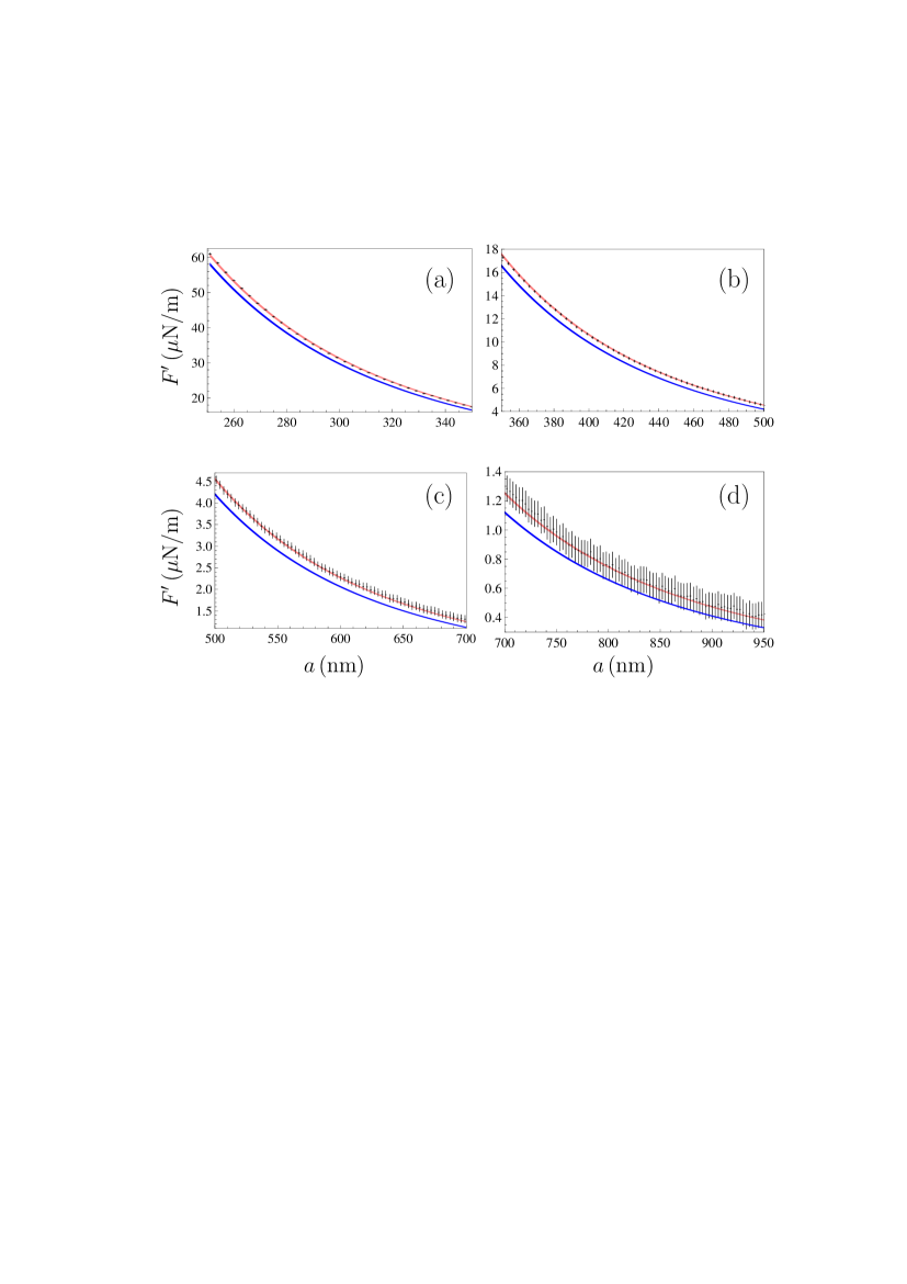
Figure 4: The mean gradient of the Casimir force obtained from the three measurement sets with small oscillation amplitude of the cantilever is shown by crosses as a function of separation within four separation intervals. For clarity only every third experimental data point is plotted. The bottom and top lines demonstrate theoretical predictions of the Lifshitz theory with inclusion and neglect of the relaxation of conduction electrons, respectively.

The measurement results for the gradient of the Casimir force obtained from the three sets are shown as crosses in Fig. 4(a-d) over the separation range from 250 to 950 nm (at larger separations the data are not informative). The vertical arms of the crosses indicate the total error in measuring the force gradient at the 67% confidence level. The horizontal arms are determined by the constant error in measuring the absolute separations $\Delta z=0.5~{}$nm. For better visualization only each third data point is plotted in Fig. 4.

We now compare experiment and theory. The thicknesses of the Au coatings on the sphere and the plate allow one to consider these bodies as made up entirely of Au in calculations of the Casimir force 1 . At the relatively large separations considered in this work, the surface roughness with rms characterized in Sec. II leads to only negligibly small contribution which can be taken into account perturbatively. For a small ratio $a/R<0.022$ the calculation of the gradient of the Casimir force can be performed within the proximity force approximation with inclusion of the first-order corrections to this approximation in $a/R$ 53a ; 52 ; 53 ; 54 ; 55 computed with inclusion of the real material properties. As a result, the gradient of the Casimir force acting between a sphere and a plate is given by

$$F_{\rm theor}^{\prime}(a)=-2\pi R\left[1+\beta(a,R)\frac{a}{R}\right]\left(1+10\frac{\delta_{s}^{2}+\delta_{p}^{2}}{a^{2}}\right)P(a),$$ (7)

where we use numerical values for the function $\beta$ computed in Ref. 55 using the extrapolation of the optical data for Au to low frequencies by means of the Drude and plasma models, and $P(a)$ is the Casimir pressure between two Au plates computed at the temperature $T=20~{}{}^{\circ}$C of the experiment. This pressure is expressed by the commonly known Lifshitz formula 1 ; 2 ; 3 ; 4 ; 5

$$P(a)=-\frac{k_{B}T}{\pi}\sum_{l=0}^{\infty}{\vphantom{\sum}}^{\prime}\!\!\int_{0}^{\infty}\!\!\!\!q_{l}k_{\bot}dk_{\bot}\!\sum_{\alpha}\frac{1}{r_{\alpha}^{-2}(i\xi_{l},k_{\bot})e^{2aq_{l}}-1}.$$ (8)

Here, $q_{l}=(k_{\bot}^{2}+\xi_{l}^{2}/c^{2})^{1/2}$, the integration is performed with respect to the magnitude of the projection of the wave vector on the plane of plates, $\xi_{l}=2\pi k_{B}Tl/\hbar$ with $k_{B}$ being the Boltzmann constant, $l=0,\,1,\,2,\,\ldots$ are the Matsubara frequencies, the summation in $\alpha$ is made over the two independent polarizations of the electromagnetic field, transverse magnetic ($\alpha={\rm TM}$) and transverse electric ($\alpha={\rm TE}$), and the reflection coefficients are expressed as

$$r_{\rm TM}(i\xi_{l},k_{\bot})=\frac{\varepsilon_{l}q_{l}-k_{l}}{\varepsilon_{l}q_{l}+k_{l}},\quad r_{\rm TE}(i\xi_{l},k_{\bot})=\frac{q_{l}-k_{l}}{q_{l}+k_{l}},$$ (9)

where the dielectric permittivity of Au is taken at the pure imaginary Matsubara frequencies $\varepsilon_{l}=\varepsilon(i\xi_{l})$ and

$$k_{l}=\left(k_{\bot}^{2}+\varepsilon_{l}\frac{\xi_{l}^{2}}{c^{2}}\right)^{1/2}.$$ (10)

Numerical computations of the gradient of the Casimir force have been performed by Eqs. (7)–(10) in the framework of the two approaches discussed in Sec. I, i.e., by using $\varepsilon_{l}$ obtained from the optical data of Au 72 extrapolated down to zero frequency by means of either the dissipative Drude or the dissipationless plasma models

$$\varepsilon_{D}(i\xi)=1+\frac{\omega_{p}^{2}}{\xi(\xi+\tau^{-1})},\quad\varepsilon_{p}(i\xi)=1+\frac{\omega_{p}^{2}}{\xi^{2}},$$ (11)

where $\hbar\omega_{p}=9.0~{}$eV and $\hbar\tau^{-1}=35~{}$meV are the energies corresponding to the plasma frequency and relaxation parameter $\gamma=\tau^{-1}$ ($\tau$ is the relaxation time) 72 .

The computational results are presented in Fig. 4(a–d) as a function of separation by the bottom and top lines obtained using the Drude and the plasma model approaches, respectively. The width of the lines characterizes the size of the theoretical error which is largerly determined by inaccuracies in the optical data of Au.

From Fig. 4 one can conclude that the theoretical predictions using the Drude model approach (i.e., taking into account the energy losses by conduction electrons) are excluded by the data over the separation range from 250 to 850 nm. As to the plasma model approach, which disregards the energy losses of conduction electrons, it is consistent with the measurement data over the entire separation region. Similar results have been obtained previously in the separation range up to 420 nm with the help of the dynamic AFM 10 ; 15 and in the separation range up to 750 nm with the help of micromechanical torsional oscillator 1 ; 2 ; 6 ; 7 ; 8 ; 9 ; 14 . In Ref. 58 only one of the three measurement sets, presented in this paper, allowed an exclusion of the Drude model approach in the region of separations from 250 to 820 nm.

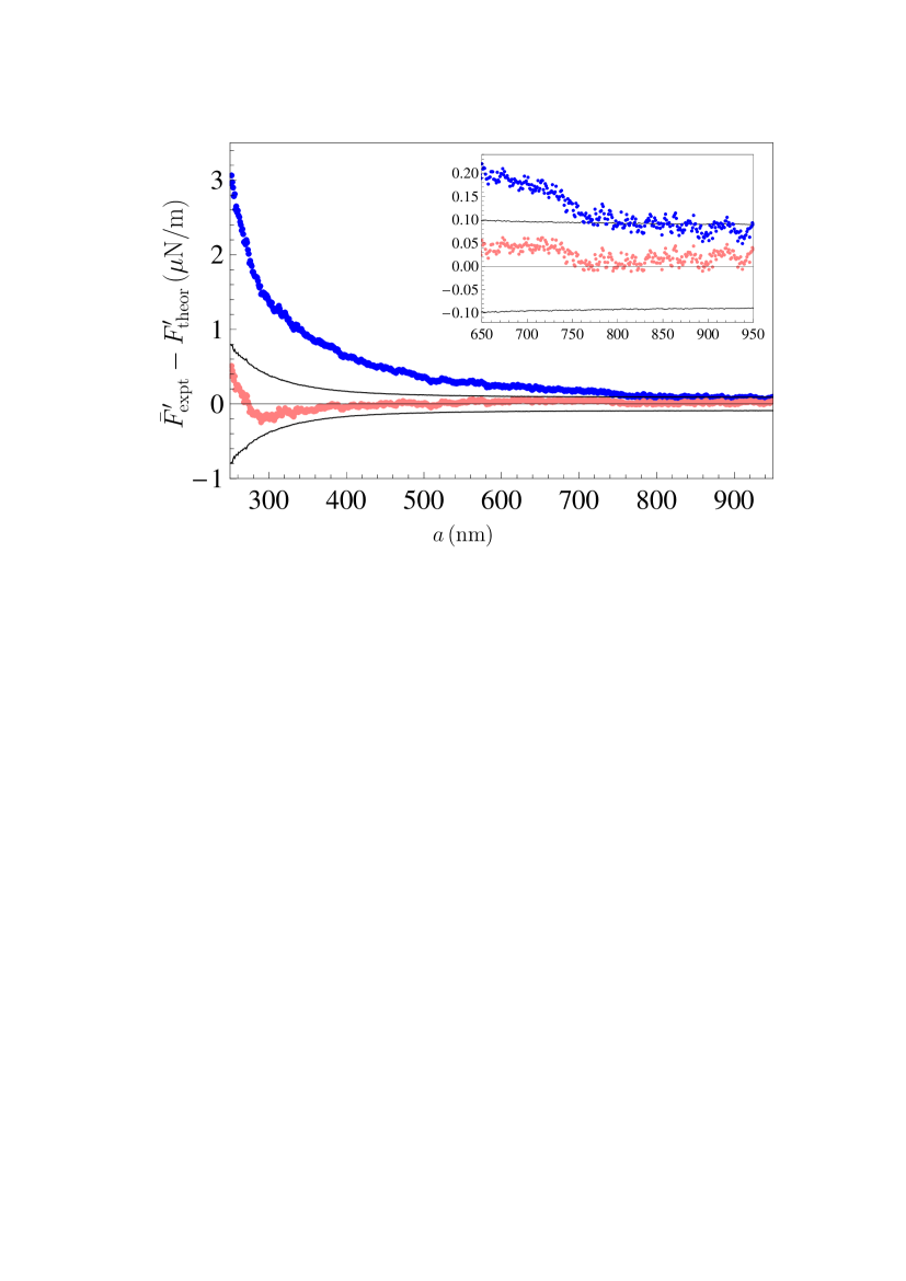
Figure 5: The differences between the mean gradient of the Casimir force obtained from the three measurement sets with small oscillation amplitude of the cantilever and theoretical gradients calculated with inclusion and neglect of the relaxation of conduction electrons are shown as functions of separations by the top and bottom sets of dots, respectively. The two lines are formed by the boundary points of the confidence intervals for the quantity $\bar{F}_{\rm expt}^{\prime}-{F}_{\rm theor}^{\prime}$. In the inset the region of separations from 650 to 950 nm is shown on an enlarged scale.

The obtained results are confirmed using another method of comparison between experiment and theory which considers the differences between mean experimental $\bar{F}_{\rm expt}^{\prime}$ and theoretical ${F}_{\rm theor}^{\prime}$ gradients of the Casimir force. These differences are plotted as dots in Fig. 5 with a step of 1 nm by the top and bottom sets found using the Drude and the plasma model approaches for ${F}_{\rm theor}^{\prime}$, respectively. In doing so the experimental gradients are the mean values obtained from the three measurement sets. The lower and upper solid lines in Fig. 5 are formed by the smoothly joined boundary points of the confidence intervals for the differences $\bar{F}_{\rm expt}^{\prime}-{F}_{\rm theor}^{\prime}$. The width of these intervals is equal to twice the total error in the quantity $\bar{F}_{\rm expt}^{\prime}-{F}_{\rm theor}^{\prime}$. The latter is found by combining in quadrature the already known total experimental error of $\bar{F}_{\rm expt}^{\prime}$ and the total theoretical error of ${F}_{\rm theor}^{\prime}$, which is determined by the errors arising from the inaccuracy of the optical data and from the calculation of the force gradient at the separation distance determined with an error $\Delta z$ (see Refs. 1 ; 7 for details). In the inset, the region of separations from 650 to 950 nm is shown on an enlarged scale.

The meaning of the confidence band in between the solid lines is the following. If the theoretical approach is consistent with the data within some separation interval at the 67% confidence level, no less than 67% of the dots in this interval should belong to the confidence band. On the other hand, the theoretical approach is excluded by the data within some interval at the same confidence level if more than 33% of the dots fall outside the confidence band 1 ; 7 ; 73 . From Fig. 5 one can see that the plasma model approach is consistent with the data over the entire measurement range from 250 to 950 nm. At the same time, the Drude model approach is excluded by the data at all separations below 850 nm (note that although some dots of the top set belong to the confidence band at separations from 770 to 850 nm, the number of these dots does not reach 67% of all the dots belonging to this interval).

Thus, the consideration of three measurement sets allows us not only to confirm the results obtained in Ref. 58 from a single set, but also to increase the upper boundary of the separation interval up to 850 nm, where the Drude model approach is excluded by the data.

IV Comparison with theory of the measurement results with larger oscillation amplitude

Next we have performed one more set of measurements of the gradient of the Casimir force with much larger separation of the closest approach between the sphere and the plate. This allows the use of a larger oscillation amplitude of the cantilever $A\approx 20$ nm while preserving the linearity of Eq. (4).

After finishing the third measurement set it was checked to confirm that the vacuum conditions in the chamber remain stable. Because of this, it was not necessary to repeat the two-step cleaning procedure done previously before each of the first three measurement sets. Measurements have been performed in the separation region from 600 nm to 2 $\mu$m in a similar way to the first three sets but the values of the applied voltages have been changed for larger ones. Ten different voltages $V_{i}$ $(i=1,\ldots,10)$ with a step of 0.01$V$ varied in the interval (–0.092 V, 0.108 V) whereas eleven fixed voltages $V_{i}$ $(i=11,\ldots,21)$ were equal to 0.008 V close to $V_{0}$.

The calibration of the setup was performed as described in Sec. III. First the residual potential difference $V_{0}$ was determined at each separation with a step of 1 nm. The obtained results are shown by the dots in Fig. 6 as a function of separation. Similar to Fig. 3, the residual potential difference is almost separation-independent. This confirms that the surfaces of both test bodies are sufficiently clean and ready for the force measurements. The best fit of the straight line $V_{0}=Ka+b$ to these data results in $K=3.23\times 10^{-4}~{}$mV/nm and $b=7.50~{}$mV in close analogy to the results obtained in the first three measurement sets (see Sec. III). The mean value of the $V_{0}$ in this case was found to be $\bar{V}_{0}=7.92~{}$mV.

Next the separation at the closest approach $z_{0}=571.9\pm 1.1~{}$nm and the calibration constant $C=(6.342\pm 0.004)\times 10^{5}~{}$s/kg were determined from the fit as described above. The latter is again in agreement with the values obtained in the first three measurement sets.

Then the 21 values of the gradient of the Casimir force at each separation with a step of 1 nm were calculated using Eq. (5). These values were averaged and the random error was found at the 67% confidence level as a function of separation. The systematic error in measurements of the frequency shift for this set was equal to $4.0\times 10^{-2}~{}$rad/s. The decrease of this error as compared to the value used in Sec. III is due to the fact that with the larger amplitude of the cantilever oscillations the corresponding interferometer signal is increased. This increases the signal-to-noise ratio leading to a reduced error in the determination of the cantilever frequency shift from the sphere-plate interaction forces. This error is used in the calculation of the systematic error in measurements of the force gradient by Eq. (4) and combined in quadrature with the random error to obtain the total experimental error in the gradient of the Casimir force $\bar{F}^{\prime}$.

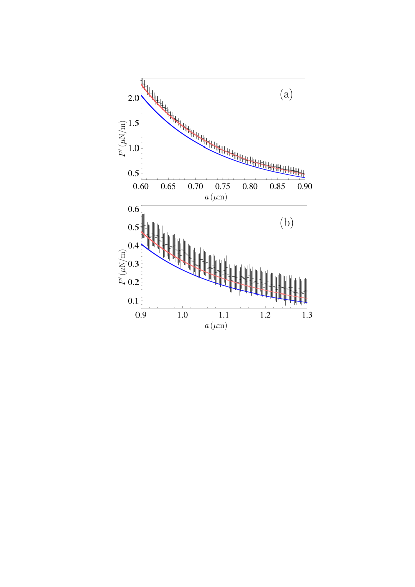
Figure 7: The mean gradient of the Casimir force obtained from the measurement set with larger oscillation amplitude of the cantilever is shown as a function of separation within two separation intervals. For clarity only every third experimental data point is plotted. The bottom and top lines demonstrate theoretical predictions of the Lifshitz theory with inclusion and neglect of the relaxation of conduction electrons, respectively.

The measured gradients are shown as crosses in Fig. 7(a,b) over the separation region from 600 nm to 1.3 $\mu$m. The arms of the crosses indicate the total error in measuring the force gradient and in measuring the absolute separations $\Delta z=1.1~{}$nm. Only each third cross is plotted in Fig. 7 to make the figure more informative.

The theoretical force gradients are computed as described in Sec. III. The computational results obtained using the Lifshitz theory and the optical data for Au extrapolated down to zero frequency by means of either the Drude of the plasma models are shown in Fig. 7 as functions of separation by the bottom and top lines, respectively. As is seen in this figure, the theoretical predictions using the dissipationless plasma model are consistent with the measurement data over the entire range from 600 nm to $1.3~{}\mu$m. From the same figure, we can conservatively conclude that the predictions of the Lifshitz theory using the dissipative Drude model for extrapolation are excluded at all separations up to $1.1~{}\mu$m. Thus, the range of separations where the Drude model is excluded by the data has been significantly extended.

Now we compare with theory the measurement data obtained at larger separations with increased oscillation amplitude using another statistical approach discussed in Sec. III. The differences between $\bar{F}_{\rm expt}^{\prime}$ and ${F}_{\rm theor}^{\prime}$ are plotted in Fig. 8 as dots with a step of 1 nm. The top and bottom sets of dots are obtained using ${F}_{\rm theor}^{\prime}$ calculated using the Drude and plasma model approaches, respectively. The two solid lines are formed by the boundary points of the confidence intervals for $\bar{F}_{\rm expt}^{\prime}-{F}_{\rm theor}^{\prime}$ determined as discussed in Sec. III. In the inset, the region of largest separations from 1 to $1.3~{}\mu$m is shown on an enlarged scale to gain a better understanding.

From Fig. 8 it is seen that all the points of the bottom set belong to the confidence interval, i.e., the plasma model approach is consistent with the data. The Lifshitz theory combined with the Drude model approach is excluded by the data over the region of separations from 0.6 to $1.1~{}\mu$m. In the intervals belonging to this range more than 33% of dots lie outside the confidence band. Therefore, the second method of comparison between experiment and theory leads to the same conclusions as the first one which means that in this experiment the region of separations where the Drude model approach is excluded is extended up to $1.1~{}\mu$m.

V Conclusions and discussion

In the foregoing, we have presented a description of the experiment on measuring the gradient of the Casimir force between metallic surfaces of a sphere and a plate cleaned by means of a two-step cleaning procedure using the UV light and Ar-ion bombardment. Compared to Ref. 58 , two additional measurement sets within the same separation range are reported here, as well as the measurement results at larger separations with a factor of two larger amplitude of the cantilever oscillations. The latter allowed one to significantly increase the range of separations where the experiment discriminates between the two theoretical approaches used in the literature on Casimir physics. Specifically, theoretical predictions based on the Lifshitz theory in combination with the dissipative Drude model for conduction electrons were excluded by the measurement data up to the separation of $1.1~{}\mu$m (to compare with 820 nm in Ref. 58 ).

As discussed in Sec. I, both the Casimir puzzle for metallic test bodies and the Casimir conundrum for dielectric and semiconductor ones are the problems which still remain to be solved. Prior to this there already was a reasonably good picture of the experimental situation concerning the Casimir puzzle at separations below a few hundred nanometers, but the situation at separations above $0.8~{}\mu$m remained completely unresolved. This made harder the theoretical solution to the problem and called for precise measurements of the Casimir interaction in the micrometer separation range. Several experiments of this kind directed to the resolution of the Casimir puzzle and Casimir conundrum have been proposed recently 74 ; 75 ; 76 ; 77 ; 78 .

The main improvements made in the experiment presented here are the use of much softer cantilever, which allowed the increase of the calibration constant by up to an order of magnitude, and implementation of the two-step cleaning procedure by means of the UV light and Ar ions, which resulted in ultra clean surfaces of both the internal walls of vacuum chamber and of the test bodies at ultrahigh ($<5\times 10^{-9}~{}\mbox{Torr}\approx 0.7\times 10^{-6}~{}$Pa) and stable vacuum. This allowed to reach low (a few mV) and stable residual potential difference which was independent of separation for the regular (not specially selected) samples. The introduction of these tools has made it possible to discriminate between the theoretical predictions with inclusion and neglect of the dissipative relaxation of conduction electrons in three measurement sets with oscillation amplitude of cantilever equal to 10 nm up to larger separation distances. As a result, the Drude model approach was excluded by the data over the separation range from 250 to 850 nm, and the plasma model approach was found to be consistent with the data.

It was checked that in the separation range from 0.6 to $2~{}\mu$m the oscillator used is still in the linear regime when the oscillation amplitude is increased to 20 nm. With this increased oscillation amplitude, the measurements of the gradient of the Casimir force have been repeated and compared with the same two theoretical approaches. It is found that the plasma model approach neglecting the relaxation of conduction electrons is again consistent with the data over the entire measurement range from 0.6 to $1.3~{}\mu$m. The Drude model approach taking into account the relaxation properties of conduction electrons was excluded over the separation range from 0.6 to $1.1~{}\mu$m. Thus, by the results of measurements with 10- and 20-nm oscillation amplitudes of the cantilever the Drude model approach is excluded by the data over the separation range from 250 to 1100 nm.

The problem of why the Lifshitz theory is in contradiction with the measurement data when it takes into account the relaxation properties of conduction electrons at low frequencies is discussed in the literature but there is yet no consensus on how this puzzle can be explained. In Refs. 58 ; 78 ; 79 it was hypothesized that a material system might not respond similarly to electromagnetic fields with nonzero field strength and to fluctuations with zero field strength but nonzero dispersion. This hypothesis does not necessarily assume a violation of the fluctuation-dissipation theorem, but might be connected with the phenomenological character of the Drude model which describes well the response of metals to real electromagnetic fields on the mass-shell but fails to give an adequate description for fluctuations that are not on the mass-shell. Future investigations will shed new light on this problem.

             

Figure 1: Schematic of the upgraded experimental setup (see text for further discussion) placed inside the vacuum chamber with a pressure $<5\times 10^{-9}~{}\mbox{Torr}\approx 0.7\times 10^{-6}~{}$Pa.

             

Figure 3: The residual potential differences between Au-coated surfaces of a sphere and a plate are shown by dots as functions of separation for (a) first, (b) second, and (c) third sets of measurements using small oscillation amplitude of the cantilever.

     

   

                          

Figure 6: The residual potential difference between Au-coated surfaces of a sphere and a plate is shown by dots as a function of separation for the set of measurements with larger oscillation amplitude of the cantilever.

   

Figure 8: The differences between the mean gradient of the Casimir force obtained from the measurement set with larger oscillation amplitude of the cantilever and theoretical gradients calculated with inclusion and neglect of the relaxation of conduction electrons are shown as functions of separations by the top and bottom sets of dots, respectively. The two lines are formed by the boundary points of the confidence intervals for the quantity $\bar{F}_{\rm expt}^{\prime}-{F}_{\rm theor}^{\prime}$. In the inset the region of separations from 1 to $1.3~{}\mu$m is shown on an enlarged scale.

References

- (1) M. Bordag, G. L. Klimchitskaya, U. Mohideen, and V. M. Mostepanenko, Advances in the Casimir Effect (Oxford University Press, Oxford, 2015).
- (2) G. L. Klimchitskaya, U. Mohideen, and V. M. Mostepanenko, The Casimir force between real materials: Experiment and theory, Rev. Mod. Phys. 81, 1827 (2009).
- (3) A. W. Rodrigues, F. Capasso, and S. G. Johnson, The Casimir effect in microstructured geometries, Nat. Photon. 5, 211 (2011).
- (4) L. M. Woods, D. A. R. Dalvit, A. Tkatchenko, P. Rodriguez-Lopez, A. W. Rodriguez, and R. Podgornik, Materials perspective on Casimir and van der Waals interactions, Rev. Mod. Phys. 88, 045003 (2016).
- (5) E. M. Lifshitz, The theory of molecular attractive forces between solids, Zh. Eksp. Teor. Fiz. 29, 94 (1955) [Sov. Phys. JETP 2, 73 (1956)].
- (6) G. L. Klimchitskaya and V. M. Mostepanenko, Experiment and theory in the Casimir effect, Contemp. Phys. 47, 131 (2006).
- (7) G. L. Klimchitskaya and V. M. Mostepanenko, Graphene may help to solve the Casimir conundrum in indium tin oxide systems, Phys. Rev. B 98, 035307 (2017).
- (8) R. S. Decca, E. Fischbach, G. L. Klimchitskaya, D. E. Krause, D. López, and V. M. Mostepanenko, Improved tests of extra-dimensional physics and thermal quantum field theory from new Casimir force measurements, Phys. Rev. D 68, 116003 (2003).
- (9) R. S. Decca, D. López, E. Fischbach, G. L. Klimchitskaya, D. E. Krause, and V. M. Mostepanenko, Precise comparison of theory and new experiment for the Casimir force leads to stronger constraints on thermal quantum effects and long-range interactions, Ann. Phys. (N.Y.) 318, 37 (2005).
- (10) R. S. Decca, D. López, E. Fischbach, G. L. Klimchitskaya, D. E. Krause, and V. M. Mostepanenko, Tests of new physics from precise measurements of the Casimir pressure between two gold-coated plates, Phys. Rev. D 75, 077101 (2007).
- (11) R. S. Decca, D. López, E. Fischbach, G. L. Klimchitskaya, D. E. Krause, and V. M. Mostepanenko, Novel constraints on light elementary particles and extra-dimensional physics from the Casimir effect, Eur. Phys. J. C 51, 963 (2007).
- (12) C.-C. Chang, A. A. Banishev, R. Castillo-Garza, G. L. Klimchitskaya, V. M. Mostepanenko, and U. Mohideen, Gradient of the Casimir force between Au surfaces of a sphere and a plate measured using an atomic force microscope in a frequency-shift technique, Phys. Rev. B 85, 165443 (2012).
- (13) A. A. Banishev, C.-C. Chang, G. L. Klimchitskaya, V. M. Mostepanenko, and U. Mohideen, Measurement of the gradient of the Casimir force between a nonmagnetic gold sphere and a magnetic nickel plate, Phys. Rev. B 85, 195422 (2012).
- (14) A. A. Banishev, G. L. Klimchitskaya, V. M. Mostepanenko, and U. Mohideen, Demonstration of the Casimir Force between Ferromagnetic Surfaces of a Ni-Coated Sphere and a Ni-Coated Plate, Phys. Rev. Lett. 110, 137401 (2013).
- (15) A. A. Banishev, G. L. Klimchitskaya, V. M. Mostepanenko, and U. Mohideen, Casimir interaction between two magnetic metals in comparison with nonmagnetic test bodies, Phys. Rev. B 88, 155410 (2013).
- (16) G. Bimonte, D. López, and R. S. Decca, Isoelectronic determination of the thermal Casimir force, Phys. Rev. B 93, 184434 (2016).
- (17) J. Xu, G. L. Klimchitskaya, V. M. Mostepanenko, and U. Mohideen, Reducing detrimental electrostatic effects in Casimir-force measurements and Casimir-force-based microdevices, Phys. Rev. A 97, 032501 (2018).
- (18) V. B. Bezerra, G. L. Klimchitskaya, and V. M. Mostepanenko, Thermodynamical aspects of the Casimir force between real metals at nonzero temperature, Phys. Rev. A 65, 052113 (2002).
- (19) V. B. Bezerra, G. L. Klimchitskaya, and V. M. Mostepanenko, Correlation of energy and free energy for the thermal Casimir force between real metals, Phys. Rev. A 66, 062112 (2002).
- (20) V. B. Bezerra, G. L. Klimchitskaya, V. M. Mostepanenko, and C. Romero, Violation of the Nernst heat theorem in the theory of the thermal Casimir force between Drude metals, Phys. Rev. A 69, 022119 (2004).
- (21) M. Bordag and I. G. Pirozhenko, Casimir entropy for a ball in front of a plane, Phys. Rev. D 82, 125016 (2010).
- (22) G. L. Klimchitskaya and V. M. Mostepanenko, Low-temperature behavior of the Casimir free energy and entropy of metallic films, Phys. Rev. A 95, 012130 (2017).
- (23) G. L. Klimchitskaya and C. C. Korikov, Analytic results for the Casimir free energy between ferromagnetic metals, Phys. Rev. A 91, 032119 (2015).
- (24) F. Chen, G. L. Klimchitskaya, V. M. Mostepanenko, and U. Mohideen, Demonstration of optically modulated dispersion forces, Opt. Express 15, 4823 (2007).
- (25) F. Chen, G. L. Klimchitskaya, V. M. Mostepanenko, and U. Mohideen, Control of the Casimir force by the modification of dielectric properties with light, Phys. Rev. B 76, 035338 (2007).
- (26) C.-C. Chang, A. A. Banishev, G. L. Klimchitskaya, V. M. Mostepanenko, and U. Mohideen, Reduction of the Casimir Force from Indium Tin Oxide Film by UV Treatment, Phys. Rev. Lett. 107, 090403 (2011).
- (27) A. A. Banishev, C.-C. Chang, R. Castillo-Garza, G. L. Klimchitskaya, V. M. Mostepanenko, and U. Mohideen, Modifying the Casimir force between indium tin oxide film and Au sphere, Phys. Rev. B 85, 045436 (2012).
- (28) G. L. Klimchitskaya and V. M. Mostepanenko, Conductivity of dielectric and thermal atom-wall interaction, J. Phys. A: Math. Theor. 41, 312002 (2008).
- (29) J. M. Obrecht, R. J. Wild, M. Antezza, L. P. Pitaevskii, S. Stringari, and E. A. Cornell, Measurement of the Temperature Dependence of the Casimir-Polder Force, Phys. Rev. Lett. 98, 063201 (2007).
- (30) B. Geyer, G. L. Klimchitskaya, and V. M. Mostepanenko, Thermal quantum field theory and the Casimir interaction between dielectrics, Phys. Rev. D 72, 085009 (2005).
- (31) G. L. Klimchitskaya and C. C. Korikov, Casimir entropy for magnetodielectrics, J. Phys.: Condens. Matter 27, 214007 (2015).
- (32) G. L. Klimchitskaya and V. M. Mostepanenko, Casimir free energy of dielectric films: classical limit, low-temperature behavior and control, J. Phys.: Condens. Matter 29, 275701 (2017).
- (33) Y. Srivastava, A. Widom, and M. H. Friedman, Microchips as Precision Quantum-Electrodynamic Probes, Phys. Rev. Lett. 55, 2246 (1985).
- (34) H. B. Chan, V. A. Aksyuk, R. N. Kleiman, D. J. Bishop, and F. Capasso, Quantum Mechanical Actuation of Microelectromechanical Systems by the Casimir Force, Science 291, 1941 (2001).
- (35) H. B. Chan, V. A. Aksyuk, R. N. Kleiman, D. J. Bishop, and F. Capasso, Nonlinear Micromechanical Casimir Oscillator, Phys. Rev. Lett. 87, 211801 (2001).
- (36) E. Buks and M. L. Roukes, Stiction, adhesion, and the Casimir effect in micromechanical systems, Phys. Rev. B 63, 033402 (2001).
- (37) E. Buks and M. L. Roukes, Metastability and the Casimir effect in micromechanical systems, Europhys. Lett. 54, 220 (2001).
- (38) J. Bárcenas, L. Reyes, and R. Esquivel-Sirvent, Scaling of micro- and nanodevices actuated by the Casimir force, Appl. Phys. Lett. 87, 263106 (2005).
- (39) G. Palasantzas, Contact angle influence on the pull-in voltage of microswitches in the presence of capillary and quantum vacuum effects, J. Appl. Phys. 101, 053512 (2007).
- (40) G. Palasantzas, Pull-in voltage of microswitch rough plates in the presence of electromagnetic and acoustic Casimir forces, J. Appl. Phys. 101, 063548 (2007).
- (41) R. Esquivel-Sirvent and R. Pérez-Pascual, Geometry and charge carrier induced stability in Casimir actuated nanodevices, Eur. Phys. J. B 86, 467 (2013).
- (42) W. Broer, G. Palasantzas, J. Knoester, and V. B. Svetovoy, Significance of the Casimir force and surface roughness for actuation dynamics of MEMS, Phys. Rev. B 87, 125413 (2013).
- (43) M. Sedighi, W. H. Broer, G. Palasantzas, and B. J. Kooi, Sensitivity of micromechanical actuation on amorphous to crystalline phase transformations under the influence of Casimir forces, Phys. Rev. B 88, 165423 (2013).
- (44) J. Zou, Z. Marcet, A. W. Rodriguez, M. T. H. Reid, A. P. McCauley, I. I. Kravchenko, T. Lu, Y. Bao, S. G. Johnson, and H. B. Chan, Casimir forces on a silicon micromechanical chip, Nat. Commun. 4, 1845 (2013).
- (45) W. Broer, H. Waalkens, V. B. Svetovoy, J. Knoester, and G. Palasantzas, Nonlinear Actuation Dynamics of Driven Casimir Oscillators with Rough Surfaces, Phys. Rev. Appl. 4, 054016 (2015).
- (46) N. Inui, Optical switching of a graphene mechanical switch using the Casimir effect, J. Appl. Phys. 122, 104501 (2017).
- (47) G. L. Klimchitskaya, V. M. Mostepanenko, V. M. Petrov, and T. Tschudi, Optical Chopper Driven by the Casimir Force, Phys. Rev. Applied 10, 014010 (2018).
- (48) F. Tajik, M. Sedighi, A. A. Masoudi, H. Waalkens, and G. Palasantzas, Sensitivity of chaotic behavior to low optical frequencies of a double-beam torsional actuator, Phys. Rev. E 100, 012201 (2019).
- (49) M. Bordag, G. L. Klimchitskaya, and V. M. Mostepanenko, The Casimir force between plates with small deviations from plane parallel geometry, Int. J. Mod. Phys. A 10, 2661 (1995).
- (50) W. Broer, G. Palasantzas, J. Knoester, and V. B. Svetovoy, Roughness correction to the Casimir force at short separations: Contact distance and extreme value statistics, Phys. Rev. B 85, 155410 (2012).
- (51) V. B. Svetovoy, P. J. van Zwol, G. Palasantzas, and J. Th. M. De Hosson, Optical properties of gold films and the Casimir force, Phys. Rev. B 77, 035439 (2008).
- (52) C. C. Speake and C. Trenkel, Forces between Conducting Surfaces due to Spatial Variations of Surface Potential, Phys. Rev. Lett. 90, 160403 (2003).
- (53) R. O. Behunin, D. A. R. Dalvit, R. S. Decca, C. Genet, I. W. Jung, A. Lambrecht, A. Liscio, D. López, S. Reynaud, G. Schnoering, G. Voisin, and Y. Zeng, Kelvin probe force microscopy of metallic surfaces used in Casimir force measurements, Phys. Rev. A 90, 062115 (2014).
- (54) C. D. Fosco, F. C. Lombardo, and F. D. Mazzitelli, Proximity force approximation for the Casimir energy as a derivative expansion, Phys. Rev. D 84, 105031 (2011).
- (55) G. Bimonte, T. Emig, R. L. Jaffe, and M. Kardar, Casimir forces beyond the proximity force approximation, Europhys. Lett. 97, 50001 (2012).
- (56) G. Bimonte, T. Emig, and M. Kardar, Material dependence of Casimir force: gradient expansion beyond proximity, Appl. Phys. Lett. 100, 074110 (2012).
- (57) G. Bimonte, Going beyond PFA: A precise formula for the sphere-plate Casimir force, Europhys. Lett. 118, 20002 (2017).
- (58) M. Hartmann, G.-L. Ingold, and P. A. Maia Neto, Plasma versus Drude Modeling of the Casimir Force: Beyond the Proximity Force Approximation, Phys. Rev. Lett. 119, 043901 (2017).
- (59) A. O. Sushkov, W. J. Kim, D. A. R. Dalvit, and S. K. Lamoreaux, Observation of the thermal Casimir force, Nat. Physics 7, 230 (2011).
- (60) V. B. Bezerra, G. L. Klimchitskaya, U. Mohideen, V. M. Mostepanenko, and C. Romero, Impact of surface imperfections on the Casimir force for lenses of centimeter-size curvature radii, Phys. Rev. B 83, 075417 (2011).
- (61) M. Liu, J. Xu, G. L. Klimchitskaya, V. M. Mostepanenko, and U. Mohideen, Examining the Casimir puzzle with an upgraded AFM-based technique and advanced surface cleaning, Phys. Rev. B 100, 081406(R) (2019).
- (62) F. J. Giessibl, Advances in atomic force microscopy, Rev. Mod. Phys. 75, 949 (2003).
- (63) E. D. Palik, O. J. Glembocki, I. Heard, P. S. Burno, and L. Tenerz, Etching roughness for (100) silicon surfaces in aqueous KOH, J. Appl. Phys. 70, 3291 (1991).
- (64) E.-L. Florin, M. Rief, H. Lehmann, M. Ludwig, C. Dornmair, V. T. Moy, and H. E. Gaub, Sensing specific molecular interactions with the atomic force microscope, Biosens. Bioelectron. 10, 895 (1995).
- (65) Y.-J. Chen, W. K. Tham, D. E. Krause, D. López, E. Fischbach, and R. S. Decca, Stronger Limits on Hypothetical Yukawa Interactions in the 30–8000 Nm Range, Phys. Rev. Lett. 116, 221102 (2016).
- (66) J. L. Garrett, D. A. T. Somers, and J. N. Munday, Measurement of the Casimir Force between Two Spheres, Phys. Rev. Lett. 120, 040401 (2018).
- (67) R. R. Sowell, R. E. Cuthrell, D. M. Mattox, and R. D. Bland, Surface cleaning by ultraviolet radiation, J. Vac. Sci. Technol. 11, 474 (1974).
- (68) J. R. Vig, UV/ozone cleaning of surfaces, J. Vac. Sci. Technol. A 3, 1027 (1985).
- (69) N. S. McIntyre, R. D. Davidson, T. L. Walzak, R. Williston, M. Westcott, and A. Pekarsky, Uses of ultraviolet/ozone for hydrocarbon removal: Applications to surfaces of complex composition or geometry, J. Vac. Sci. Technol. A 9, 1355 (1991).
- (70) D. E. King, Oxidation of gold by ultraviolet light and ozone at 25 ∘C, J. Vac. Sci. Technol. A 13, 1247 (1995).
- (71) A. Krozer and M. Rodahl, X-ray photoemission spectroscopy study of UV/ozone oxidation of Au under ultrahigh vacuum conditions, J. Vac. Sci. Technol. A 15, 1704 (1997).
- (72) S. R. Koebley, R. A. Outlaw, and R. R. Dellwo, Degassing a vacuum system with in-situ UV radiation, J. Vac. Sci. Technol. A 30, 060601 (2012).
- (73) Handbook of Adhesive Technology, eds. A. Pizzi and K. L. Mittal, 2nd Edition (Marcel Dekker, New York, 2003).
- (74) H. Lüth, Surfaces and Interfaces of Solid Materials (Springer, Berlin, 2015).
- (75) W. R. Smythe, Electrostatics and Electrodynamics (McGraw-Hill, New York, 1950).
- (76) S. G. Rabinovich, Measurement Errors and Uncertainties: Theory and Practice (AIP Press, Springer, New York, 2000).
- (77) Handbook of Optical Constants of Solids, ed. E. D. Palik (Academic, New York, 1985).
- (78) V. M. Mostepanenko, How to confirm and exclude different models of material properties in the Casimir effect, J. Phys.: Condens. Matter 27, 214013 (2015).
- (79) G. Bimonte, G. L. Klimchitskaya, and V. M. Mostepanenko, Universal experimental test for the role of free charge carriers in the thermal Casimir effect within a micrometer separation range, Phys. Rev. A 95, 052508 (2017).
- (80) R. Sedmik and P. Brax, Status Report and first Light from Cannex: Casimir Force Measurements between flat parallel Plates, J. Phys.: Conf. Ser. 1138, 012014 (2018).
- (81) G. L. Klimchitskaya, V. M. Mostepanenko, R. I. P. Sedmik, and H. Abele, Prospects for Searching Thermal Effects, Non-Newtonian Gravity and Axion-Like Particles: CANNEX Test of the Quantum Vacuum, Symmetry 11, 407 (2019).
- (82) G. Bimonte, Apparatus to probe the influence of the Mott-Andersen metal-insulator transition in doped semiconductors on the Casimir effect, Phys. Rev. A 99, 052506 (2019).
- (83) G. L. Klimchitskaya, V. M. Mostepanenko, and R. I. P. Sedmik, Casimir pressure between metallic plates out of thermal equilibrium: Proposed test for the relaxation properties of free electrons, Phys. Rev. A 100, 022511 (2019).
- (84) G. L. Klimchitskaya and V. M. Mostepanenko, Casimir energy and pressure for magnetic metal films, Phys. Rev. B 94, 045404 (2016).