A Generalized Rate-Distortion-$\lambda$ Model Based HEVC Rate Control Algorithm

Abstract

The High Efficiency Video Coding (HEVC/H.265) standard doubles the compression efficiency of the widely used H.264/AVC standard. For practical applications, rate control (RC) algorithms for HEVC need to be developed. Based on the R-Q, R-$\rho$ or R-$\lambda$ models, rate control algorithms aim at encoding a video clip/segment to a target bit rate accurately with high video quality after compression. Among the various models used by HEVC rate control algorithms, the R-$\lambda$ model performs the best in both coding efficiency and rate control accuracy. However, compared with encoding with a fixed quantization parameter (QP), even the best rate control algorithm [1] still under-performs when comparing the video quality achieved at identical average bit rates.

In this paper, we propose a novel generalized rate-distortion-$\lambda$ (R-D-$\lambda$) model for the relationship between rate (R), distortion (D) and the Lagrangian multiplier ($\lambda$) in rate-distortion (RD) optimized encoding. In addition to the well designed hierarchical initialization and coefficient update scheme, a new model based rate allocation scheme composed of amortization, smooth window and consistency control is proposed for a better rate allocation. Experimental results implementing the proposed algorithm in the HEVC reference software HM-16.9 show that the proposed rate control algorithm is able to achieve an average of BDBR saving of 6.09%, 3.15% and 4.03% for random access (RA), low delay P (LDP) and low delay B (LDB) configurations respectively as compared with the R-$\lambda$ model based RC algorithm [1] implemented in HM. The proposed algorithm also outperforms the state-of-the-art algorithms, while rate control accuracy and encoding speed are hardly impacted.

I Introduction

HEVC [2] is the latest video compression standard from ITU and MPEG as the successor to H.264/AVC [3]. It has been widely observed that HEVC can save 50% of the bits on average as compared to H.264/AVC while achieving the same visual quality, at a cost of much higher encoding complexity [4]. Even though video can be encoded using the constant quantization parameter (CQP) mode, also known as the non-RC mode, in practical applications, rate control is more commonly used to encode an input video to a target bit rate for bandwidth constrained applications while achieving good video quality after compression.

Rate control can be generally categorized into two types, constant bit rate (CBR) control and average bit rate (ABR) control. ABR sets a target average bit rate for the entire video or every single video segment while allowing the bit rate to vary among different parts of the video according to the complexity of those parts. On the other side, CBR requires a strictly uniform output bit rate for every time period, typically one second. At a given bit rate, ABR usually provides a higher quality after compression than CBR, as CBR sacrifices a lot in coding efficiency for constant bit rates over time. ABR is usually used in coding efficiency oriented applications like video on demand and video storage, while CBR is often used in jitter-sensitive applications like video call and satellite based video communication. This paper focuses on proposing a novel ABR algorithm to improve the coding efficiency of HEVC, so only ABR is discussed and tested in this paper.

In general, rate control algorithms need to achieve a high bit rate accuracy as measured by bit rate error, while achieving good video coding efficiency, which is generally measured by BDBR [5]. On a high level, rate control consists of two steps,

1. allocating the target bit rate across and inside frames of the input sequence,

2. selecting proper coding parameters to meet the target bit rate with good video quality.

Existing rate control algorithms for HEVC typically use one of three rate estimation models, namely the R-Q model [6, 7], the R-$\rho$ model [8, 9], and the R-$\lambda$ model [10, 1]. These models were designed to predict the output bit rate R after compression using features such as the quantization $Q$ in the R-Q model, the percentage of zero-valued transformed coefficients $\rho$ in the R-$\rho$ model and the Lagrangian multiplier $\lambda$ in the R-$\lambda$ model.

Experiments show that R-$\lambda$ model based rate control algorithms [10, 1] significantly outperform the R-Q model and R-$\rho$ model based algorithms. The first R-$\lambda$ model based rate control algorithm [10] is 15% better in coding efficiency than the previous state-of-the-art R-Q model based rate control algorithm [7] with a nearly halved bit rate error. As a result, R-$\lambda$ model based algorithms [10, 1] have been adopted and integrated in the HEVC reference software. However, as mentioned in [10, 1], the coding efficiency of the current R-$\lambda$ model based rate control algorithm is still much lower than the CQP mode. In addition, Wen et al [11] pointed out that the current R-$\lambda$ model based rate control algorithm might fail when meeting scene changes.

To improve the performance of R-$\lambda$ model based rate control, many algorithms [12, 13, 14, 15, 16, 11, 17] have been proposed to improve rate allocation and/or model coefficients update mechanisms. These algorithms achieve a higher coding efficiency than the original R-$\lambda$ model based RC algorithm proposed in [10, 1]. However, those algorithms mainly focus on improving the rate allocation and model coefficients update based on the R-$\lambda$ model without further improving the R-$\lambda$ model.

In this paper, we propose a novel generalized rate-distortion-$\lambda$ model to better model the relationship between rate, distortion and $\lambda$. The proposed algorithm improves the accuracy of model fitting by 56% over R-$\lambda$ model. Besides the new model, the well designed hierarchical initialization and the model coefficients update scheme, a new model based rate allocation scheme is proposed for a better rate allocation. The rate allocation module includes amortization for I frame, smooth window based compensation and consistency control on QP value selection. Experimental results implementing the proposed algorithm in the HEVC reference software HM-16.9 show that the proposed rate control algorithm is able to produce average BDBR savings of 6.09%, 3.15% and 4.03% for the Random Access (RA), Low Delay P (LDP) and Low Delay B (LDB) configurations respectively as compared with the R-$\lambda$ model based RC algorithm in [1], i.e. the default RC algorithm in HM. The proposed algorithm also outperforms the state-of-the-art rate control algorithms, while the rate control accuracy and encoding speed are hardly impacted.

The remainder of this paper is organized as follows. Sec. II reviews the research on HEVC rate control. Sec. III describes the proposed algorithm in detail. Sec. IV presents experimental results. Section V concludes the paper.

II Related Work

II-A Rate Control Models

In HEVC encoding, the quantization parameter (QP) and the Lagrangian multiplier $\lambda$ for rate-distortion optimization (RDO) are two important parameters that directly determine output video quality and bit rate after compression. QP decides the quantization step that is used to quantize the residual after transform, which determines the distortion of each predicting mode as well as the residual after quantization. $\lambda$, as a function of QP, defines the following RDO target function in [18],

$$J=min(D+\lambda\cdot R),$$ (1)

where $J$ is also known as the RD cost. It has been widely agreed that the following logarithmic relationship [19] between QP and $\lambda$ can achieve the best encoding efficiency statistically.

$$QP=c_{1}\times ln(\lambda)+c_{2},$$ (2)

where $c_{1}$ and $c_{2}$ are variables related to the video characteristics and compression performance. Based on this relationship, rate control algorithms only need to decide either QP or $\lambda$. Then various models are used to estimate the coding parameters according to the target bit rate.

The R-Q model assumes that the quantization step $Q$ has a direct correspondence to the coding complexity and can accurately estimate the number of bits consumed using the following quadratic model [6],

$$R = aQ^{-1}+bQ^{-2},$$ (3)

$$QP = 12.0+6.0\times log(Q/0.85),$$ (4)

where $a$ and $b$ are two parameters related to video content that are updated as encoding proceeds. Choi et al [7] proposed a pixel based unified R-Q model based rate control algorithm for HEVC, which was adopted and implemented in HEVC reference software HM-8.0. As discussed, $Q$ can only determine the distortion and residual of each predicting mode. However, $\lambda$ decides which prediction mode to use, while the output bit rate of the current prediction is determined by CABAC. Therefore, the indirect relationship between R and Q cannot achieve a high accuracy in rate estimation. In addition, the non-monotonic quadratic model in R-Q model is hard to be accurately updated during the encoding process, which would also reduce the coding efficiency.

Another class of rate control algorithms, namely $\rho$ domain rate control [20, 8, 9], assumes a linear relationship, shown in Equation (5), between the output bit rate and the percentage of zeros among the quantized transform coefficients, denoted as $\rho$.

$$R=\theta\cdot(1-\rho).$$ (5)

$\rho$ domain rate control algorithms were popular for H.264. However, HEVC standard introduces a flexible quad-tree coding unit (CU) partition scheme and the skip prediction method, leading to significant difference in the distribution of zeros after transform and quantization. In addition, the extra bits consumed by newly introduced syntaxes also make the linear relationship between $\rho$ and output bit rate less accurate as compared with H.264. As a result, $\rho$ domain rate control is rarely used in HEVC.

As the state of the art, Li et al [10] proposed a novel R-$\lambda$ model for HEVC, where the relationship between distortion and rate is modelled as a hyperbolic function in Equation (6). Accordingly, the relationship between bit per pixel (bpp) and $\lambda$ is also hyperbolic after unit conversion, as given in Equation (7).

$$D = CR^{-K},$$ (6)

$$\lambda = \alpha bpp^{\beta},$$ (7)

where $C$, $K$, $\alpha$ and $\beta$ are content related parameters. Only $\alpha$ and $\beta$ are needed to be estimated and updated during encoding. Similar to the hierarchical structure used in HEVC, $\lambda$ domain rate control algorithms also propose its own hierarchy, where frames in the same frame-reference hierarchy share a same set of model coefficients. During encoding, $\alpha$ and $\beta$ are updated using a least mean square based gradient descent scheme. Experimental results [10] show that R-$\lambda$ model is able to properly model the relationship between distortion and rate with a coefficient of determination ($r^{2}$) value around 0.995. Compared with R-Q model based rate control algorithm [7], the former state of the art, R-$\lambda$ model based rate control algorithm [10] improves the coding efficiency by 15.9% for LD and 24.6% for RA respectively. As a result, the R-$\lambda$ model based rate control algorithm in [10] was adopted and implemented in the HEVC reference software HM-10.0. However, experimental results in [10] also show that the coding efficiency of the R-$\lambda$ model based algorithm is still far inferior to CQP.

II-B Bit Allocation

The R-$\lambda$ model in Equation (7) is highly effective for output rate estimation and determining the QP value to hit a target bit rate. However, the question of optimally allocating the total bit rate budget to frames and/or CUs for a higher video coding efficiency remains open.

Li et al [1] proposed a largest coding unit (LCU)-level separate model based block level bit allocation scheme, which achieves a higher rate control accuracy and also a higher coding efficiency (2.8% and 3.9% for LD and RA) than [10]. As a result, the algorithm was incorporated into HEVC reference software HM-11.0.

As LD configuration and RA configuration are very different from each other in rate distribution, some rate allocation algorithms were designed to work with only one of the two configurations. For example, [15] was predominantly designed to work very well in the RA mode, whereas [12] is among the best for LD. RA uses a more complex reference hierarchy that needs to adapt to input content, so it is generally more difficult for RC algorithms to work well with RA.

Xie et al [13] proposed a temporal dependent bit allocation scheme which allocates bit rate according to the complexity of each coding tree unit (CTU). Results show a coding efficiency improvement of 1.78% over [10] for LD. Wang [14] et al proposed a new relationship between the distortion and $\lambda$ for a better rate regulation and a higher consistency in quality with an average gain of 0.37 dB in PSNR. Li et al [12, 16] proposed a recursive Taylor expansion method to iteratively estimate a close form of the optimal rate allocation, which improved the coding efficiency by 2.2% and 2.4% on average over [1] for LDP and LDB respectively.

As to RA configuration, Song et al [21] proposed a group of pictures (GOP) level rate allocation scheme to accurately match the HEVC GOP coding structure in RA, which achieves a coding efficiency that is 0.2% higher than [1]. Gong et al [22] proposed a temporal-layer-motivated lambda domain picture level rate control algorithm to better estimate the influence of each layer, which leads to an average gain of 3.87% in coding efficiency as compared with [1]. He et al [15] proposed an inter-frame dependency based dynamic programming method for frame level bit allocation, which improves the coding efficiency by 5.19% on average for RA than [1] with an increase of 0.41% in encoding time .

II-C Other methods

Besides rate allocation, various schemes have been proposed for a better RC performance, such as adaptive quantization, new RC models and multi-pass encoding.

Adaptive quantization is another mean of bit allocation, which usually first uses traditional RC algorithms to decide a central QP value. The QP values for frames and CUs are adjusted later. Tang et al [23] proposed a Hadamard energy feature for adaptive quantization and achieved 3.3% gain in coding efficiency as compared with [1].

Lee et al [17] proposed a Laplacian probability density function to derive a new model between rate and distortion. The coding performance is slightly better than [10] but worse than [1], so this model was not adopted by HEVC reference software.

Besides only using features inside a frame, there are also some multi-pass methods, which increases the coding efficiency at a cost of higher latency and higher computing complexity. Wen et al [11] proposed a pre-compression based double update scheme to better handle scene changes, which achieves an average gain in PSNR of 0.1dB for common single-scene test sequences and up to 4.5dB for complicated multi-scene videos. The macroblock-tree algorithm proposed in [24] was designed to adjust the QP value according to the frequency at which a block is directly and indirectly referenced. An extra pass of encoding is required in the macroblock-tree algorithm, which leads to a higher latency and a higher complexity. Based on the macroblock-tree algorithm, Yang et al [25] proposed a low-delay source distortion temporal propagation model, which improves the coding efficiency of H.264 reference software JM by 15%. Fiengo et al [26] proposed a convex optimization based recursive R-D model, which achieves a gain of 12% in coding efficiency as compared with [10] with a 10x-50x higher encoding time. Ropert et al [27, 28] proposed a sequential two-pass method for a better rate allocation, which results in an increase of 16% in coding efficiency at a cost of an average increase of 57% in encoding time as compared with [1].

III The Proposed Algorithm

In this section, we describe in detail, the proposed generalized rate-distortion-$\lambda$ model, and the proposed rate control algorithm based on the new model, including the hierarchical initialization, least mean square based update scheme and the rate allocation module.

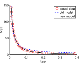
(a) PeopleOnStreet 1600p

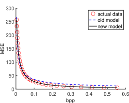
(b) PartyScene 480p

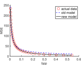
(c) BlowingBubbles 240p

Figure 1: R-D Curves Fit Using the Two Different Models

III-A Rate-Distortion-$\lambda$ Model

The core of the R-$\lambda$ model can be found in Equation (6) and (7). Though the model performs well in R-D fitting, there are two implied assumptions that are invalid under border conditions in real world applications, namely, (a) infinite bit rate when distortion is zero, (b) infinite distortion when bit rate is zero rate.

HEVC provides a lossless encoding mode, where the QP value is 4 and the corresponding quantization step is 1. Therefore, the output rate of lossless encoding is the minimum bit rate for the video to be encoded without distortion. Such lossless bit rate is not much greater than output bit rate values from lossy encodings. For example, the lossless bit rate of Kimono in class B is 3.3 bpp, and that of FourPeople in class F is 2.2 bpp. A common target bit rate of lossy encoding usually lies in the range between 0.01 bpp and 0.5 bpp, which is only one to two orders of magnitude smaller than the rate of lossless encoding. Therefore, such border cases cannot be ignored in the model. On the other side, zero rate encoding can be approximated by only storing the average value of the video, where the output distortion is the variance of the video.

These two boundary cases prove that a more realistic rate-distortion model must intercept both the rate axis and the distortion axis. This is, however, not true for the R-$\lambda$ model, which manifests as loss of model accuracy, especially for very low/high bit rates.

According to the discussion above, the proposed model is given as follows,

$$D = max(0,C(R+B)^{-K}-T)$$ (8)

$$\approx C(R+B)^{-K}-T,$$ (9)

where $C$ and $K$ are parameters similar to their name sakes in the traditional R-$\lambda$ model that represent the basic characters of the video. According to the results in [10], $K$ is usually around 1. $B$ is the parameter describing the interception on the distortion axis. The distortion of zero bit rate encoding can be described by $CB^{-K}$, which equals to the variance of the video. As a result, $B$ is usually much smaller than a typical target bit rate. $T$ is the parameter for the interception on the rate axis, which equals to $C(R_{lossless}+B)^{-K}$ and usually is one to two orders of magnitude smaller than typical output distortion. The model can be simplified to Expression (9) if only lossy encoding is considered.

The modelling performance between rate and distortion, i.e. how close the model could fit the regression curve to the actual data, determines how accurately the model could possibly be updated. Therefore, a fitting experiment was conducted to evaluate the expressive power of the proposed new model in describing the relationship between rate and distortion, where test sequences in HEVC common test condition [29] (class A to E, 20 videos in total) were encoded using the CQP mode with QP values from 4 to 51 tested to cover all possible output rates. When QP is set to 4, the quantization step is 1 in encoding, which represents lossless encoding and also the highest possible output rate. 51 is the greatest QP value that is allowed in HEVC, which leads to a lowest possible output rate. For each video sequence, the relationship between distortion (measured by mean squared error, MSE) and rate (measured by bpp) were fit using the rate-distortion model [10] in Equation (6) and the proposed model defined in Equation (9).

TABLE I: RD Curves Fitting Performance

QP Range	Model	$r^{2}$			RMSE
		worst	avg	std	worst	avg	std
4…51	[10]	0.9504	0.9925	0.0106	11.24	3.03	2.91
	Proposed	0.9777	0.9966	0.0055	7.62	1.32	1.62
4…22	[10]	0.9046	0.9831	0.0242	1.59	0.32	0.36
	Proposed	0.9763	0.9940	0.0074	0.36	0.15	0.11
17…37	[10]	0.8904	0.9880	0.0252	9.89	1.47	2.10
	Proposed	0.9603	0.9941	0.0108	2.65	0.65	0.72
32…51	[10]	0.9818	0.9978	0.0040	8.24	2.14	2.37
	Proposed	0.9880	0.9992	0.0027	6.90	0.76	1.47

Table I gives the fitting results of the model used in R-$\lambda$ model and the proposed model with coefficient of determination ($r^{2}$) and root mean square error (RMSE) used as the metrics. $r^{2}$ describes how close the actual data is to the fitted regression curve. RMSE is the standard deviation of the prediction residues. A higher $r^{2}$ value or a lower RMSE value for a same set of data suggests a better fitting.

In the experiment, four QP ranges (namely, full QP range: 4…51, low QP range: 4…22, middle QP range: 17…37, high QP range: 32…51) were tested to compare the expressive powers of two models for different QP ranges. Each of the sub-ranges contains around 20 points to guarantee a similar difficulty in fitting. As shown in Table I, for the full QP range (4…51), the proposed model is able to improve $r^{2}$ value from 0.9925 to 0.9966 on average, with RMSE reduced from 3.03 to 1.32, i.e. a 56% reduction. It should be noted that the $r^{2}$ values in the proposed experiment are lower than the results in [10] because 48 data points (QP from 4 to 51) were used in our experiment, while only four points (QP in {22, 27, 32, 37}) were used in [10]. Furthermore, the proposed model is intended for both the average and worst cases for full QP range, while the much lower standard deviations (std) of $r^{2}$ and RMSE show that the proposed model is more robust than the model in [10] when handling different kinds of videos.

In addition, the results in Table I prove that the proposed model outperforms the R-$\lambda$ model for all three sub-ranges of QP values. The R-$\lambda$ model sometimes produces very low $r^{2}$ values for low QP values. As discussed above, a common target bit rate of lossy encoding is only one to two orders of magnitude smaller than the rate of lossless encoding. As a result, the proposed model greatly benefits from the refinement on the zero-distortion boundary case and therefore produces a much higher and stabler fitting performance. On the other side, the distortion of zero rate encoding, i.e. the variance of the video, is usually much greater than the distortion after compression, so the gain in $r^{2}$ for the high QP range due to the zero-rate boundary case is expected to be smaller than that for the low and middle QP ranges. The R-$\lambda$ model is already very accurate for the high QP range, while the proposed model still provides a similar improvement in RMSE for the high QP range as compared with other ranges. It should be noted that $r^{2}$ and RMSE both increase for the high QP range as compared with the low and middle QP ranges because RMSE is proportional to distortion. So RMSE increases for the high QP range due to a much greater distortion in spite of a higher $r^{2}$ value.

Fig. 1 gives three examples of the RD curves fitted using the two models. The original data points are plotted in distinct red circles, while the curves fitted using the old model and the proposed model are plotted using blue dashed line and black solid line respectively. It needs to be noted that the model coefficients were estimated using all data points in the full QP range, while only a part of data points (QP 15 to 44) is plotted in Fig. 1 to prevent the large range making the plot hard to discern. As can be seen from the figure, the R-$\lambda$ model performs well for high QP values and starts to deteriorate with a lower QP value, while the proposed model is able to accurately predict the RD relationship for all cases.

Based on the proposed rate-distortion model defined in Equation (9), the proposed R-D-$\lambda$ model can be derived as follows,

$$\lambda = -\frac{\partial D}{\partial R}=CK(R+B)^{-K-1}$$ (10)

$$= \alpha(bpp+\gamma)^{\beta},$$ (11)

$$bpp = (\frac{\lambda}{\alpha})^{1/\beta}-\gamma,$$ (12)

$$\alpha = CK,$$ (13)

$$\beta = -K-1,$$ (14)

$$\gamma = \frac{B}{W\times H\times Fr},$$ (15)

where $\lambda$ is the opposite number of the derivative between distortion and rate. Equation (11) and (12) provide another two interpretations of Equation (10) with the unit of rate converted from bits to bpp. $\alpha$, $\beta$ and $\gamma$ are the short codes of the video characters related parameters with definitions given in Equation (13)-(15). These three parameters are updated using the algorithm proposed in Sec. III-C as coding proceeds. $W$, $H$ and $Fr$ are the width, height and frame rate of the video.

Based on the model definition introduced above, $\lambda$ can be calculated according to the target bit rate. And the value of QP can be calculated using the logarithmic function defined in Equation (2). The values of $c_{1}$ and $c_{2}$ in Equation (2) were determined through a tuning experiment where various values were tested to cooperate with the remaining parts of the proposed algorithm. It was found that the following QP-$\lambda$ relationship provided the best coding efficiency for the HEVC common test condition, and therefore is used in the proposed algorithm.

$$QP=round(4.3\times ln(\lambda)+14.6).$$ (16)

III-B Hierarchical Initialization

Similar to [10], in the proposed algorithm, frames of a same reference hierarchy share a same set of model coefficients, which is updated after every encoding of frame. All CUs inside a frame share the model of that frame without separate maintenance. The update mechanism of the model coefficients is introduced in Sec. III-C.

In [10], the initial values of $\alpha$ and $\beta$ are set to 3.2003 and -1.367 respectively, which are the averaged fitted values using the sequences in the HEVC common test condition. It is agreed that the initial values of model coefficients do not have an overall significant influence on the coding efficiency as long as model coefficients can be properly updated during encoding. However, it is still beneficial to set the initial values according to the reference frame hierarchy.

TABLE II: RA Coding Structure in HEVC

FrameNum	POC	Level	Ref Num	QP Offset	$\lambda$ Multiplier
1	8	1	3	1	0.442
2	4	2	3	2	0.3536
3	2	3	4	3	0.3536
4	1	4	4	4	0.68
5	3	4	4	4	0.68
6	6	3	3	3	0.3536
7	5	4	4	4	0.68
8	7	4	4	4	0.68

TABLE III: LD Coding Structure in HEVC

FrameNum	POC	Level	Ref Num	QP Offset	$\lambda$ Multiplier
1	1	3	4	3	0.4624
2	2	2	4	2	0.4624
3	3	3	4	3	0.4624
4	4	1	4	1	0.578

Figure 2: R-D Curves of Different Frame Levels

A hierarchically structured GOP mechanism with frames at different levels of the hierarchy using different numbers of reference frames and different QP values was proposed in HEVC. In general, a smaller QP value is used for frames of a lower level, which are referenced more and reference other frames less. The hierarchical structures of HEVC (RA in Table III, LD in Table III) were carefully designed and fine-tuned for a statistically optimal coding efficiency under the HEVC common test condition. Intra-picture coded frames (I frames) belong to frame level 0, while inter-picture coded frames (P frames and B frames) are categorized into frame level 1 to 4 in RA. A lower frame level represents a higher importance in the reference structure and a lower dependence on other frames in coding and therefore a usually lower coding efficiency. Fig. 2 gives the RD curves of different frame levels of “PartyScene” from class C, which was encoded by HM-16.9 using RA configuration with QP values from 22 to 37. As shown in Fig. 2, for a given output quality, frames of frame level 4 only require about 25% of the bit rate that is needed by frames of frame level 1. Therefore, it is not proper to set the initial values of all frame levels to the same value.

To derive a close form of the optimal relationship between model parameters and frame level, it is assumed that when a video sequence is encoded to a bit rate of $R$ by encoder A and a certain quality, encoder B would encode that video into a similar quality if the output bit rate is $dR$, where $d$ is the relative coding efficiency between encoder B and encoder A over a range of bit rates. This assumption is widely used in many encoder evaluation schemes, such as the BDBR metric [5]. In this paper, it is assumed that the linear scaling of difference in coding efficiencies between two encoders is applicable to the coding efficiencies of two frame levels as well. The distortions when encoding a frame at two different frame levels ($i$ and $j$) by the same encoder can be modelled by

$$D = C_{i}(R+B_{i})^{-K_{i}}-T_{i}$$ (17)

$$= C_{j}(dR+B_{j})^{-K_{j}}-T_{j},$$ (18)

where $d$ is the relative coding efficiency between level $j$ and $i$. $T_{i}$ is the feature same in Expression (9), which equals to $C_{i}(R_{i,lossless}+B_{i})^{-K_{i}}$ and is one to two orders smaller than that in lossy encoding cases. The difference between $T_{i}$ and $T_{j}$ is much smaller than common distortion and therefore can be ignored. As introduced earlier, $B$ is usually much smaller than practical bit rates so that Expression (19) and (21) can be approximated using Taylor expansion. According to the results in [10], $K$ is usually around 1 so that $K$ will not affect the order of magnitude of $\frac{B}{R}$. So $\frac{B_{i}B_{j}}{R^{2}}$ in Expression (22) is much smaller than 1, and therefore can be ignored to get the final approximation. The entire approximation is described as follows,

$$C_{i}(R+B_{i})^{-K_{i}} \approx C_{j}(dR+B_{j})^{-K_{j}}$$ (19)

$$C_{i}R^{-K_{i}}(1-\frac{K_{i}B_{i}}{R}) \approx C_{j}(dR)^{-K_{j}}(1-\frac{K_{j}B_{j}}{dR})$$ (20)

$$R^{{K}_{j}-{K}_{i}} \approx \frac{C_{j}}{C_{i}}{d}^{-{K}_{j}}\frac{1-\frac{K_{j}B_{j}}{dR}}{1-\frac{K_{i}B_{i}}{R}}$$ (21)

$$\approx \frac{C_{j}}{C_{i}}{d}^{-{K}_{j}}(1-\frac{K_{i}K_{j}B_{i}B_{j}}{dR^{2}})$$ (22)

$$\approx \frac{C_{j}}{C_{i}}{d}^{-{K}_{j}}$$ (23)

To ensure Expression (23) roughly holds for a wide range of rates to satisfy the assumption, $K_{i}$ and $K_{j}$ must be very close to each other, while the $C$ values for different frame levels roughly follows a reciprocal relationship of the relative coding efficiency of each frame level.

$$\frac{C_{j}}{C_{i}}\approx{d}^{K}\approx d$$ (24)

TABLE IV: $C$ for Different Frame Levels in RA

Frame Level	1 (P frame)	2	3	4
Ref Distance	8	4	2	1
$C$	4.180	2.905	1.892	1.020

Wang et al [30] concludes that coding efficiency decreases as a logarithmic function of the distance between the current frame and the reference, which is highly consistent with the fitted results of the RD curves of different frame levels given in Table IV. It should be noted that the logarithmic relationship is not a good fit for frame level 1 (P frames), as frames in level 1 only allows uni-directional prediction, while frames of higher frame levels can be encoded using bi-directional prediction that improves the coding efficiency.

Moreover, the hierarchical initialization scheme for $\gamma$ can be obtained using the zero rate encoding case, where the theoretical maximum distortion is the variance, which is similar for frames within one scene. Therefore, the hierarchical initialization scheme for $\gamma$ can be derived as follows,

$$C_{i}{B_{i}}^{-K} \approx C_{j}{B_{j}}^{-K}$$ (25)

$$(\frac{B_{j}}{B_{i}})^{K} \approx \frac{C_{j}}{C_{i}}\quad\approx d^{K}$$ (26)

$$\frac{\gamma_{j}}{\gamma_{i}} \approx \frac{C_{j}}{C_{i}}\quad\approx d$$ (27)

In summary, the model coefficients of different frame levels are initialized hierarchically, while frames of the same frame level share the same set of model coefficients. For the RA configuration, all frame levels share the same $\beta$ value of -1.35, while $\alpha$ and $\gamma$ follow a fixed proportional relation of [4.2:3:2:1] from the results in Table IV for frame level 1 to 4 with center values (frame level 2) set to 4.4 and 0.005 for $\alpha$ and $\gamma$ respectively. For the LD configuration, $\beta$ is also set to -1.35, while $\alpha$ and $\gamma$ are set to 2.4 and 0.005 for frame level 1 to 3. 0.005 is the averaged fitted values of $\gamma$ using the sequences in HEVC common test condition. A $\gamma$ value of 0.005 (i.e. 140kbps for 720p@30fps and 60kbps for 480p@30fps) is usually much lower than practical target bit rates. It is still possible that $\gamma$ is comparable with the target bit rate for very simple videos. In those cases, the relationship that $B$ is much smaller than target bit rate will not sustain and the approximations like Expression (21) will fail. To ensure this relationship, the initial $\gamma$ is clipped by 0.1 times of the target bit rate as the upper bound.

III-C Model Parameters Update Scheme

In the proposed rate control algorithm, frames of a same frame level share a same set of model coefficients, which is updated after every encoding of a frame. Unlike the LCU-level separate model proposed in [1], the proposed algorithm only allows separate models for different frame levels. CUs inside a frame share the model of this frame, which will not be updated until this frame is completely encoded. In the proposed algorithm, each frame is first allocated with a target bit rate, denoted as $bpp_{0}$. The estimated coding parameter $\lambda$ (denoted as $\lambda_{0}$) can be calculated using

$$\lambda_{0}=\alpha_{i}(bpp_{0}+\gamma_{i})^{{\beta}_{i}},$$ (28)

where $i$ is the frame level of the current frame. The corresponding QP value ($QP_{0}$) can be calculated using Equation (16).

After the current frame is encoded, the output bit rate ($bpp_{1}$) can be observed, which is used to update the proposed R-D-$\lambda$ model using the least mean square (LMS) update rule. The $\lambda$ estimation for hitting a target bit rate can be considered a regression problem, where $bpp_{0}$ is the input variable, and $\lambda_{0}$ is the estimated output. Then ($bpp_{1}$, $\lambda_{0}$) becomes an actual data point of the model, while $\lambda_{1}$ is the estimated biased output, which can be calculated as follows.

$$\lambda_{1}=\alpha_{i}(bpp_{1}+\gamma_{i})^{{\beta}_{i}}.$$ (29)

To make the power function easy to be updated in gradient descent, a squared logarithmic error ($e^{2}$) is used as follows,

$$e^{2} = \frac{1}{2}(ln\lambda_{0}-ln\lambda_{1})^{2},$$ (30)

$$ln\lambda_{1} = ln\alpha_{i}+\beta_{i}ln(bpp_{1}+\gamma_{i})$$ (31)

The derivatives between $e^{2}$ and $\alpha$, $\beta$ as well as $\gamma$ can be calculated as follows,

$$\frac{\partial{e^{2}}}{\partial{\alpha_{i}}} = \frac{\partial{e^{2}}}{\partial{ln\lambda_{1}}}\frac{\partial{ln\lambda_{1}}}{\partial{ln\alpha_{i}}}\frac{\partial{ln\alpha_{i}}}{\partial{\alpha_{i}}}$$ (32)

$$= -(ln{\lambda}_{0}-ln{\lambda}_{1})\frac{\partial{ln{\lambda}_{1}}}{\partial{ln\alpha_{i}}}\frac{\partial{ln\alpha_{i}}}{\partial{\alpha_{i}}}$$

$$= -(ln{\lambda}_{0}-ln{\lambda}_{1})\frac{1}{\alpha_{i}}$$

$$\frac{\partial{e^{2}}}{\partial{\beta_{i}}} = -(ln{\lambda}_{0}-ln{\lambda}_{1})\frac{\partial{ln{\lambda}_{1}}}{\partial{\beta_{i}}}$$ (33)

$$= -(ln{\lambda}_{0}-ln{\lambda}_{1})ln(bpp_{1}+\gamma_{i})$$

$$\frac{\partial{e^{2}}}{\partial{\gamma_{i}}} = -(ln{\lambda}_{0}-ln{\lambda}_{1})\frac{\partial{ln{\lambda}_{1}}}{\partial{\gamma_{i}}}$$ (34)

$$= -(ln{\lambda}_{0}-ln{\lambda}_{1})\frac{\beta_{i}}{bpp_{1}+\gamma_{i}},$$

Based on the LMS update rule, the model coefficients can be updated using the updating strength set ($\sigma_{\alpha}$, $\sigma_{\beta}$, $\sigma_{\gamma}$) as follows. The symbols with a dot symbol above are the coefficients after update.

$$\dot{\alpha_{i}} := \alpha_{i}+\sigma_{\alpha}(ln{\lambda_{0}}-ln{\lambda_{1}})\frac{1}{\alpha_{i}},$$ (35)

$$\dot{\beta_{i}} := \beta_{i}+\sigma_{\beta}(ln{\lambda_{0}}-ln{\lambda_{1}})ln(bpp_{1}+\gamma_{i}),$$ (36)

$$\dot{\gamma_{i}} := \gamma_{i}+\sigma_{\gamma}(ln{\lambda_{0}}-ln{\lambda_{1}})\frac{\beta_{i}}{bpp_{1}+\gamma_{i}}.$$ (37)

In the proposed algorithm, the initial update strengths of $\alpha$, $\beta$ and $\gamma$ are set to 0.05, 0.2 and 0.000001 times of the target bpp, which gradually decrease during the encoding process using a decay scheme. Inspired by the decreasing learning rate schemes that are widely used in deep learning applications, an exponential decay scheme is used in the proposed algorithm for a better convergence and noise reduction. In the proposed algorithm, each frame level maintains a set of model coefficients as well as a decay value, which is multiplied by 0.99 after a frame of that level is encoded. Furthermore, the efficient scene change detection algorithm proposed in our previous work [23] is included in the proposed algorithm. If a scene change is observed, the model parameters are reset to initial values and the decay value is reset to 1. It should be noted that the videos in the HEVC common test condition do not include scene changes, so the scene change detection module was disabled in the experiment.

III-D Rate Allocation

The rate allocation scheme in the proposed algorithm can be separated into two levels, GOP level and picture level. CUs inside a frame share a same set of coding parameters for a spatially consistent output quality. The rates mentioned in this section are all measured in bpp.

As a special case, I frames are usually very different from inter-picture coded frames in terms of R-D relationship, so there is usually a special rate control module for I frames. Similar as [10, 1], the proposed rate allocation module first treats I frames as inter-picture coded frames and obtain a target bit rate for that frame. Then the algorithm in [31] is used to refine the target bit rate and get a new target bit rate as well as a new set of coding parameters. As I frames usually consume a bit rate that is much higher than the average target bit rate, Li et al [1] proposed a smooth window scheme to mitigate the overflow in bit rate consumption, where the rate overflow is compensated in the next smooth window (typically 40 frames) at any instant moment. The smooth window scheme works well for most cases, but it may fail in the cases with excessive bit consumption. In addition, the compensation will be unbalanced if the planned intra period and the length of smooth window are not aligned.

To solve this problem, an amortization and smooth window joint scheme with restriction on maximum bit rate for I frames is designed in the proposed rate control algorithm. “Amortization” is a process where the “debt”, i.e. the excessive consumption of bit rate caused by I frame encoding, is paid off (i.e. compensated) by the remaining non-I frames within the current intra period. For example, an I frame (frame number $i$) is first considered as a P frame and allocated with a target bit rate ($R_{i0}$). $R_{i0}$ is refined using the algorithm in [31] into a new target bit rate $R_{i1}$, which is restricted to be not greater than half of the target rate consumption of the intra period. After encoding, the I frame is encoded into a different number of bits $R_{i2}$. The rate to be recorded (denoted as $R_{i3}$, which is $R_{i0}$ for I frames and $R_{i2}$ for non-I frames) is used in the smooth window module, while the overhead of I frames (i.e. $R_{i2}-R_{i0}$) is amortized by the remaining non-I frames within the current intra period as follows,

$$R_{am}=\frac{R_{i2}-R_{i0}}{IntraPeriod-1},$$ (38)

where $R_{am}$ is the averaged amortized rate compensation for each frame, and $IntraPeriod$ is the length of the current intra period. It needs to be noted that I-frames overhead is amortized in a weighted manner rather than in a uniform way. Details are introduced in the frame level rate allocation part. $R_{am}$ is an averaged compensation to make the calculation easier. On top of the amortization scheme, the smooth window module proposed in [1] only accumulates and compensates the overflow caused by non-I frames.

Given the current status of amortization, the proposed GOP level bit allocation first deducts the target amortization from the average target bit rate. Then the overflow caused by non-I frames is compensated uniformly for each GOP within a smooth window, which is set to 40 frames in the proposed algorithm. According to the description, the target bit rate of the current GOP (${R}_{GOP}$) can be calculated as follows.

$$R_{of} = \sum_{i=0}^{N-1}{(R_{i3}-R_{i0})}$$ (39)

$${R}_{GOP} = ({R}_{avg}-R_{am}-\frac{R_{of}}{SW}){N}_{GOP}.$$ (40)

$R_{of}$ is the accumulated non-I rate overflow of the $N$ frames that have been encoded. $SW$ is the length of the smooth window. $R_{avg}$ is the average target bit rate, and ${N}_{GOP}$ is the length of the current GOP.

Within the GOP, the target bit rate for each frame is allocated in a weighted manner, aiming at a sensible hierarchical quality distribution. As the output bit rate can be estimated by Equation (12), the optimal frame level rate allocation can be considered as an optimal central $\lambda$ selection problem, which is introduced as follows,

$$\underset{\lambda}{min}(abs(\sum_{i=0}^{N_{GOP}-1}{max(R_{i0},minRate)}-R_{GOP})),$$ (41)

$$R_{i0}=(\frac{\lambda\omega_{i}}{\alpha_{i}})^{1/\beta_{i}}-\gamma_{i},$$ (42)

where $\alpha_{i},\beta_{i},\gamma_{i}$ are the model coefficients for frame $i$. $\lambda$ is the central $\lambda$ value to be solved, and $\omega_{i}$ is the $\lambda$ multiplier for each frame. $abs(.)$ is the absolute value function. Same as [10], $minRate$ of one frame is set to 100 bits as the minimum achievable number of bits in the proposed algorithm. Similar to the hierarchical scheme introduced in Sec. III-B, frames of a same frame level share the same value of $\omega$.

Based on Equation (10), the relationship between D and $\lambda$ can also be interpreted in the forms of Equation (43) and (44)

$$(\frac{D}{C})^{\frac{K+1}{K}} = R^{-K-1}=\frac{\lambda}{CK},$$ (43)

$$D^{\frac{K+1}{K}} = \frac{\lambda}{K}C^{\frac{1}{K}},$$ (44)

$$D^{2} \approx \lambda C.$$ (45)

Expression (45) is approximated from Equation (44) based on the fact that $K$ is usually close to 1, which was mentioned in [10]. Table IV shows that the relationship among the $C$ coefficients for different frame levels of RA follows a proportional relationship of [4.2:3:2:1]. Therefore, a reciprocal relationship of $\lambda$ would roughly produce a similar output quality for frames of different frame levels. As the hierarchical structure was designed to encode a more important frame into a better quality, the proposed rate allocation algorithm uses a relationship of [1:2.5:4.5:10] for the $\omega$ values for different frame levels in RA. After the $\omega$ values are specified, the optimization in Expression (41) can be solved using an iterative binary search. The corresponding $\omega$ values for LD are set to [1:4:5]. The fixed values above were selected through an experiment, which tried various values to cooperate with the remaining parts of the proposed algorithm for a higher coding efficiency.

After the frame level coding parameters are determined, CUs inside a frame share the same set of coding parameters, which may slightly reduce the accuracy of rate control but improve coding efficiency and spatial consistency in output quality.

III-E Consistency Control

After $\lambda$ value is specified, QP can be calculated using Equation (16). To guarantee the output quality to be consistent over time, $\lambda$ and QP must not change significantly. Therefore, a constraint on the maximum QP difference between different frames is used. The maximum QP difference between two consecutive frames of a same frame level is set as 3, while the maximum QP difference between two consecutive encoded frames is 10.

TABLE V: RD Performance for RA Configuration, CQP as Anchor

Clip	[7]		[10]-Frame		[10]-LCU		[1]-Frame		[1]-LCU		[15]		Proposed
	BDBR	$\Delta$R	BDBR	$\Delta$R	BDBR	$\Delta$R	BDBR	$\Delta$R	BDBR	$\Delta$R	BDBR	$\Delta$R	BDBR	$\Delta$R
A_NebutaFestival	9.55	0.62	14.20	0.88	14.78	0.57	4.06	0.43	2.97	0.20	-2.94	1.53	3.74	0.79
A_PeopleOnStreet	44.35	0.74	41.95	0.96	50.13	0.26	18.13	0.05	24.91	0.01	22.30	1.22	1.57	0.27
A_SteamLoco	202.06	0.77	62.31	2.96	54.93	3.05	44.76	3.20	46.29	3.69	43.65	2.46	45.57	3.91
A_Traffic	65.00	1.49	6.03	0.60	6.06	0.52	1.20	0.77	4.57	0.87	0.55	0.56	0.77	1.51
B_BasketballDrive	33.22	0.87	4.65	0.65	7.78	0.61	2.00	0.67	6.60	0.57	-0.26	0.43	-1.84	0.43
B_BQTerrace	57.54	0.40	3.74	0.88	5.76	0.67	3.88	1.44	7.44	0.93	5.01	2.11	-0.37	1.79
B_Cactus	76.00	0.53	0.86	0.09	1.60	0.04	1.71	0.06	3.18	0.03	-3.13	1.60	-2.48	0.03
B_Kimono	44.72	1.30	8.86	0.13	10.18	0.07	8.08	0.23	9.86	0.45	3.81	0.83	8.91	0.41
B_ParkScene	54.72	0.96	2.95	0.13	5.28	0.38	2.74	0.31	3.14	0.03	-3.18	1.09	0.01	0.68
C_BasketballDrill	58.56	0.50	3.81	1.14	3.60	1.12	1.41	1.22	0.58	1.06	-2.52	0.76	-3.37	0.71
C_BQMall	87.82	0.43	15.87	1.07	18.38	0.65	13.52	1.04	12.55	0.60	8.55	0.67	4.74	1.23
C_PartyScene	102.03	0.23	10.89	0.54	13.59	0.54	4.77	0.50	3.94	0.29	-0.64	0.42	0.04	0.51
C_Racehorses	48.13	1.03	14.23	0.05	16.46	0.09	7.12	0.06	9.61	0.05	4.15	1.22	2.67	0.01
D_BasketballPass	27.64	0.42	6.75	0.72	9.91	1.01	3.82	0.73	4.75	1.05	2.74	0.70	0.16	0.56
D_BlowingBubbles	70.31	0.73	17.77	1.73	25.97	0.75	10.95	1.11	15.25	0.61	9.27	1.16	2.45	1.54
D_BQSquare	91.74	0.42	7.22	1.05	8.99	1.01	5.01	1.28	5.88	1.03	-1.02	2.54	0.30	0.96
D_Racehorses	44.49	1.13	10.13	0.27	12.56	0.20	3.40	0.34	4.44	0.24	-2.76	2.00	-0.56	0.20
Average	65.76	0.74	13.66	0.81	15.65	0.68	8.03	0.79	9.76	0.69	4.92	1.25	3.67	0.92
Average Without *	57.24	0.74	10.62	0.68	13.19	0.53	5.74	0.64	7.48	0.50	2.50	1.18	1.05	0.73

TABLE VI: RD Performance for LDP Configuration, CQP as Anchor

Clip	[7]		[10]-Frame		[10]-LCU		[1]-Frame		[1]-LCU		[12]		Proposed
	BDBR	$\Delta$R	BDBR	$\Delta$R	BDBR	$\Delta$R	BDBR	$\Delta$R	BDBR	$\Delta$R	BDBR	$\Delta$R	BDBR	$\Delta$R
B_BasketballDrive	17.70	0.54	0.54	0.64	7.37	0.61	0.53	0.64	4.51	0.54	4.44	0.62	3.60	0.64
B_BQTerrace	53.03	0.79	0.38	1.27	1.09	1.15	0.32	1.25	5.84	1.05	0.70	1.10	0.58	1.21
B_Cactus	42.82	0.11	-5.61	0.10	-4.42	0.03	-5.56	0.04	-2.13	0.02	-5.23	0.02	-8.29	0.04
B_Kimono	33.48	0.30	8.65	0.51	14.10	0.03	6.96	1.72	9.21	0.03	6.14	0.03	6.51	0.81
B_ParkScene	39.82	0.43	1.25	0.23	4.82	0.04	0.63	0.78	2.37	0.04	0.66	0.02	1.00	0.57
C_BasketballDrill	11.51	1.32	-5.43	1.32	-3.95	1.21	-5.39	1.35	-5.78	1.24	-6.13	1.29	-7.53	1.35
C_BQMall	22.38	1.18	7.08	1.09	9.08	1.02	7.08	1.09	7.48	1.04	6.51	0.99	5.74	1.06
C_PartyScene	69.89	1.51	2.16	0.69	7.43	0.70	2.17	0.69	2.77	0.59	1.32	0.62	2.45	0.66
C_Racehorses	20.67	0.07	7.63	0.29	14.84	0.57	7.79	0.11	9.94	0.07	9.38	0.07	8.31	0.06
C_BasketballPass	9.85	1.72	1.33	1.05	7.94	1.05	1.39	1.04	2.20	1.00	2.21	1.30	2.38	1.09
D_BlowingBubbles	21.22	1.13	1.09	1.05	7.62	1.02	1.08	1.04	2.28	0.94	0.57	0.87	2.53	1.00
D_BQSquare	41.05	1.87	1.26	1.53	7.42	1.42	1.26	1.57	2.13	1.42	1.43	1.40	-0.35	1.50
D_Racehorses	10.25	0.13	2.69	0.29	7.73	0.26	2.75	0.21	3.48	0.18	3.12	0.18	3.14	0.18
E_FourPeople	19.18	0.58	6.28	0.08	11.87	0.06	6.18	0.18	2.25	0.08	-2.85	0.05	-8.10	0.16
E_Johnny	70.91	0.47	12.79	0.15	27.62	0.06	12.80	0.12	6.67	0.06	1.83	0.05	-5.39	0.09
E_Kristen&Sara	37.86	0.20	5.81	0.08	15.48	0.07	5.80	0.09	0.31	0.10	-6.28	0.11	-11.33	0.09
Average	32.60	0.77	2.99	0.65	8.50	0.58	2.86	0.74	3.35	0.52	1.11	0.54	-0.30	0.66

TABLE VII: RD Performance for LDB Configuration, CQP as Anchor

Clip	[7]		[10]-Frame		[10]-LCU		[1]-Frame		[1]-LCU		[12]		Proposed
	BDBR	$\Delta$R	BDBR	$\Delta$R	BDBR	$\Delta$R	BDBR	$\Delta$R	BDBR	$\Delta$R	BDBR	$\Delta$R	BDBR	$\Delta$R
B_BasketballDrive	19.04	0.61	5.62	0.69	8.64	0.67	0.94	0.69	4.93	0.58	5.01	0.66	3.58	0.68
B_BQTerrace	76.62	0.77	1.71	1.48	4.69	1.35	3.38	1.48	8.64	1.25	2.78	1.29	1.38	1.43
B_Cactus	46.83	0.13	-4.81	0.10	-3.52	0.03	-4.16	0.05	-1.03	0.03	-4.22	0.02	-8.26	0.04
B_Kimono	35.64	0.28	11.81	0.55	13.58	0.03	6.48	1.71	8.52	0.02	5.57	0.02	5.74	0.84
B_ParkScene	41.17	0.42	2.38	0.32	4.93	0.06	0.95	0.77	2.76	0.05	0.94	0.04	1.10	0.64
C_BasketballDrill	38.42	1.67	-6.33	1.33	-3.32	1.25	-4.77	1.40	-5.39	1.25	-5.56	1.29	-7.00	1.37
C_BQMall	22.42	1.15	9.32	1.10	9.54	1.06	7.86	1.12	7.81	1.07	6.56	1.02	6.18	1.08
C_PartyScene	58.28	1.21	4.89	0.70	8.13	0.70	2.40	0.69	3.05	0.60	1.56	0.63	1.71	0.68
C_Racehorses	20.98	0.04	13.31	0.26	15.53	0.51	8.04	0.06	10.63	0.03	10.32	0.02	8.39	0.05
C_BasketballPass	8.72	1.63	5.65	1.09	8.22	1.11	1.63	1.12	2.17	1.03	2.49	1.35	2.55	1.12
D_BlowingBubbles	19.75	1.18	4.94	1.05	7.66	1.03	0.91	1.02	2.00	0.93	0.02	0.87	2.19	1.03
D_BQSquare	41.26	1.67	8.06	1.56	10.93	1.48	2.85	1.62	3.66	1.42	3.02	1.45	0.61	1.47
D_Racehorses	10.30	0.13	7.03	0.28	8.63	0.18	3.15	0.14	3.62	0.12	3.34	0.12	3.30	0.14
E_FourPeople	19.21	0.71	14.76	0.10	12.53	0.07	6.77	0.20	3.07	0.08	-2.21	0.07	-7.44	0.19
E_Johnny	69.72	0.71	34.84	0.37	30.70	0.26	16.58	0.34	9.64	0.26	2.95	0.26	-2.68	0.31
E_Kristen&Sara	39.79	0.22	18.94	0.08	15.94	0.10	7.26	0.08	1.55	0.10	-5.16	0.10	-10.30	0.09
Average	35.51	0.78	8.26	0.69	9.55	0.62	3.77	0.78	4.10	0.55	1.71	0.57	0.07	0.70

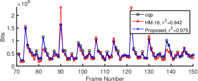
(a) PeopleOnStreet Bits

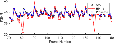
(b) PeopleOnStreet PSNR

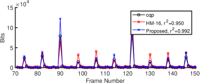
(c) BlowingBubbles Bits

(d) BlowingBubbles PSNR

Figure 3: Per-Frame Bits and PSNR for PeopleOnStreet and BlowingBubbles

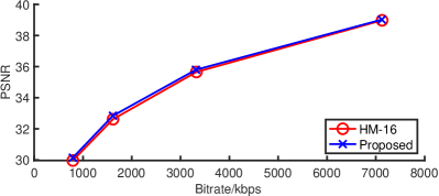
(a) RA, PartyScene, 480p

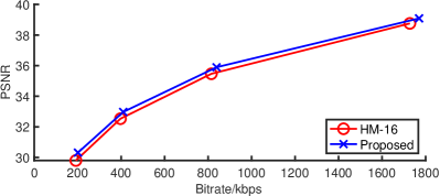
(b) RA, BlowingBubbles, 240p

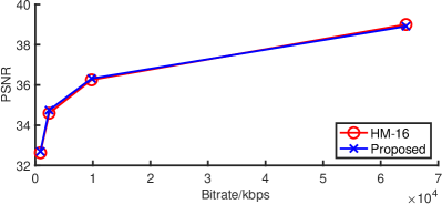
(c) LDP, BQTerrace, 1080p

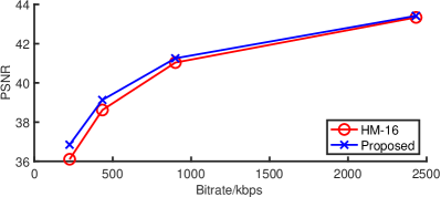
(d) LDP, FourPeople, 720p

(e) LDB, Cactus, 1080p

(f) LDB, Johnny, 720p

Figure 4: Comparisons of the RD Curves for Different Sequences

IV Experimental Results

IV-A Experiments Set-Up

To evaluate the performance of the proposed algorithm, the proposed algorithm was implemented in the HEVC reference software HM-16.9. Besides the proposed algorithm, the state-of-the-art rate control algorithms [7, 10, 1, 12, 15] were also tested in the experiment. It should be noted that the algorithms in [10] and [1] provide two modes each, allowing LCU-level separate model or not. The corresponding results of two modes are denoted with suffix Frame/LCU in the tables. The default setting of HM enables LCU-level separate model. It is found that the rate control algorithm in HM is able to achieve a higher coding efficiency and a higher bit rate error without LCU-level separate model, so the two modes were both tested in the experiments.

The HEVC common test condition [29] is used as the core test of the proposed experiment. All 20 videos (roughly 10 seconds each) in class A to E of HEVC common test condition are used as the test sequences to cover videos of various video characteristics. According to the HEVC common test condition, the sequences in class B, C, D and E are tested for the LD test, including low delay P (LDP) configuration and low delay B (LDB) configuration, while the sequences in classes A, B, C and D are tested in the RA test. As instructed in the common test condition, the test sequences were first encoded by HM-16.9 using the CQP mode (QP in {22,27,32,37}) and three configurations to generate the target average bit rates of the later rate control (ABR) encoding. The results of the CQP mode are also used as the anchor of the comparison, which is widely accepted as the statistical upper limit of the coding efficiency that one-pass rate control algorithms can approach.

Then different rate control algorithms were used to encode the test sequences into the corresponding target bit rates generated by the CQP mode. As to the state-of-the-art algorithms, it should be noted that the algorithm in [12], the best rate control algorithm for LDP and LDB configurations, was designed dedicated for LD, while the algorithm in [15], so far the best RC algorithm for RA, was solely proposed for RA. As a result, the algorithms in [12] and [15] were only tested for LD and RA respectively.

As instructed in the HEVC common test condition, the algorithms were evaluated using two metrics, PSNR based coding efficiency and rate control accuracy in sequence level. Four points of encoding results (bit rate and MSE based YUV PSNR) were used to calculate the BDBR between the CQP mode and RC algorithms. BDBR was proposed in [5], which estimates the delta bit rate that is needed for the current codec to achieve a same quality as compared with the anchor codec. A negative value of BDBR suggests an average bit rate saving for a given quality after compression, i.e. gain in coding efficiency. Rate control accuracy was measured by the averaged absolute bit rate error per sequence using the following formula:

$$\Delta R=\frac{|R_{out}-R_{target}|}{R_{target}}\times 100,$$ (46)

where $|.|$ operator is to get the absolute value. The experiments were conducted on a server with dual Intel Xeon CPU E5-2695 v2 without optimization on parallelism and SIMD.

To better evaluate the performance of the proposed algorithm, subjective quality (SSIM[32]) based coding efficiency (BDBR-SSIM) is also analyzed in the proposed experiment besides the HEVC common test condition which only compares the objective quality (PSNR) based coding efficiency.

In the subjective experiment, BDBR-SSIM results are used to evaluate the performance of the proposed algorithm. SSIM value is designed to lie in the range of [0, 1], a greater SSIM value suggesting a better subjective quality. However, SSIM is not a distance metric, which is usually first translated into a dB value (${SSIM}_{dB}$) using Equation (47) for a better fitting in the BDBR tool, especially when SSIM values are very close to 1.

$${SSIM}_{dB}=min(-10*{log}_{10}(1-ssim),100),$$ (47)

In addition, the respective impact caused by the modules in the proposed algorithm are also tested and discussed, including objective and subjective quality based coding efficiency as well as computing complexity.

IV-B Performance for HEVC Common Test Condition

Table VII gives the results of various algorithms for RA. The default algorithm in HM ([1]-LCU) is 9.76% worse than the CQP mode, while the state-of-the-art RC algorithm for RA [15] reduces the gap to 4.92% at a cost of nearly doubled rate control error. The proposed algorithm is only 3.67% away from CQP, while the rate control error is 0.92%, which is much lower than [15]. It should be noted that among the test sequences, SteamLoco (marked with $*$ in Table VII) is an outlier due to its extremely high complexity. SteamLoco is a video captured by a moving camera, which contains a running steam locomotive with plenty of billowing steam, i.e. rich and volatile texture with limited temporal similarity. Therefore, SteamLoco is not suitable for hierarchical schemes which were built based on the assumption of high temporal similarity. None of the algorithms is able to properly handle this video, and the BDBR losses of various RC algorithms over CQP are all around 45%. The BDBR results of SteamLoco are much greater than other videos, which has a significant influence on the average results. Therefore, the bottom row of Table VII also provides the averaged results without SteamLoco to better compare the performance on other videos. Under that criterion, the proposed algorithm is only 1.05% worse than the CQP mode, while the algorithms in [1]-LCU and [15] are 5.74% and 2.50% worse than the CQP mode.

Table VII and VII give the results of the LDP and LDB configurations. Experimental results show that the proposed algorithm is on average 0.30% better than CQP for LDP and only 0.07% worse than CQP for LDB with a very low bit rate error. The proposed algorithm is the first rate control algorithm that is able to reach the statistically upper limit of the coding efficiency of single-pass rate control algorithms for LD. On the other side, [1]-LCU, the default RC algorithm in HM, is 3.35% and 4.10% worse than CQP for LDP and LDB, while the best RC algorithm for LD in [12] is 1.11% and 1.71% worse than CQP for LDP and LDB respectively. It should be noted that the results of [12] is slightly different from the results in their paper, because a different setting of option “KeepHierarchicalBit” was used in [12]. In the experiment of [12], option “KeepHierarchicalBit” was set to 1 for the anchor configuration, while the default setting in HM-16.9 is 2, which outperforms 1 in coding efficiency.

It should be noted that the proposed algorithm achieves a better coding efficiency than the CQP mode for some videos. This result is not against the claim that the coding efficiency of the CQP mode is the “statistical” upper limit of single-pass RC algorithms. The coefficients in the QP-$\lambda$ relationship in Equation (2) and the hierarchical structures are statistically optimal for the HEVC common test condition, which are not necessarily optimal for any single video. As a result, it is possible that a RC algorithm produces a rate allocation and coding parameters selection scheme that is closer to the per-sequence optimum than the CQP mode.

Fig. 4 gives some examples of per-frame rate consumption and PSNR using the proposed algorithm, the default RC algorithm in HM [1] and the CQP mode, where $r^{2}$ is the correlation coefficient between the output per-frame rates of RC algorithms and CQP. The CQP mode is usually considered as the statistical upper bound of the coding efficiency of single-pass rate control algorithms, because the CQP mode was designed to encode a video into a reasonable distribution of quality after compression. The output per-frame rates of CQP mode suggest a favorable distribution of per-frame rates to hit the favorable distribution of quality after compression. As a result, a higher correlation indicates a better rate allocation. Fig. 4-(a) and 4-(c) show that the proposed algorithm is able to produce per-frame rates that are much closer to the CQP output than [1]. Fig. 4-(b) gives an example of improper overflow compensation of [1], which causes a significant quality deterioration after a frame that consumes too many bits. On the contrary, the proposed algorithm encodes that part into a more temporally consistent quality. Fig. 4 gives some examples of RD curves comparison for different configurations, which show that the proposed algorithm is able to steadily improve the coding efficiency for a wide range of bit rates. Fig. 4-(d) and 4-(f) show that the proposed algorithm is able to provide a higher gain for the cases targeting very low bit rates.

IV-C Module-level Subjective and Objective Performance

The proposed module-level experiment includes objective and subjective performance evaluation as well as complexity analysis. As some modules in the proposed algorithm are designed to work with the proposed R-D-$\lambda$ model, like the new update scheme, it is hard to test and analyze those modules separately. Therefore, the module-level analysis is conducted in an incremental way. The proposed algorithm is separated into four phases, namely,

1. Phase 1: The proposed R-D-${\lambda}$ model in Equation (11) is used to replace the model used in [10] with the QP-$\lambda$ relation in Equation (16). The model coefficients are updated using the update scheme proposed in [10].

2. Phase 2: The proposed hierarchical initialization scheme is implemented on top of Phase 1.

3. Phase 3: The proposed rate allocation scheme is implemented on top of Phase 2.

4. Phase 4: The proposed update scheme is used to replace the update scheme proposed in [10] on top of Phase 3. Phase 4 is the proposed algorithm.

TABLE VIII: Per-module Analysis of the Proposed Algorithm

HM-RC[1] as Anchor		Phase 1	Phase 2	Phase 3	Phase 4
RA	BDBR-PSNR	-4.35%	-4.37%	-4.49%	-5.44%
	BDBR-SSIM	-1.26%	-1.48%	-1.48%	-2.16%
	$\Delta$T	+1.70%	+1.74%	+1.70%	+1.67%
LDP	BDBR-PSNR	-1.68%	-1.75%	-3.27%	-3.62%
	BDBR-SSIM	-0.88%	-1.41%	-2.76%	-3.13%
	$\Delta$T	+1.10%	+0.69%	-0.08%	+0.18%
LDB	BDBR-PSNR	-1.78%	-1.79%	-3.54%	-3.93%
	BDBR-SSIM	-0.85%	-1.34%	-2.98%	-3.42%
	$\Delta$T	+0.99%	+0.63%	+0.01%	-0.40%

Table VIII shows the performance of each phase of the proposed algorithm. The proposed R-D-$\lambda$ model (Phase 1) provides the majority of the gain in objective quality based coding efficiency (BDBR-PSNR), which is 4.35%/5.44% for RA, 1.68%/3.62% for LDP and 1.78%/3.93% for LDB. The gain caused by the proposed model is higher for RA than LD because RA allows bi-directional referencing with more available reference frames, which greatly increases the coding efficiency of the frames of a higher frame level. The gap between the bit rates of lossy encoding and lossless encoding is lower for RA than LD, so the proposed model brings a higher gain for RA.

In addition, the proposed algorithm results in a similar gain in subjective quality based coding efficiency, though the parameters in the proposed algorithm was tuned using BDBR-PSNR, which proves that the proposed algorithm is effective for improving both the objective and subjective quality after compression.

Table VIII also provides the results on the complexity change caused by the proposed algorithm. An increase of 0.5% in complexity is observed on average for three configurations, which is usually within the range of measurement noise and therefore can be considered negligible.

V Conclusion and Discussion

In this paper, we propose a novel generalized R-D-$\lambda$ model to better model the relationship between rate, distortion and $\lambda$. Based on the new model, a novel average bit rate control (ABR) scheme for HEVC is designed, which includes hierarchical initialization, LMS based update for model coefficients as well as amortization and smooth window joint rate allocation. Experimental results of implementing the proposed algorithm into the HEVC reference software HM-16.9 shows that the proposed rate control algorithm is able to achieve the best coding efficiency among the state-of-the-art RC algorithms, which is only 3.67% and 0.07% worse than CQP for RA and LDB configurations and 0.3% better than CQP for LDP, while rate control accuracy and encoding speed are hardly impacted.

In future, we will keep investigating the following issues. The proposed algorithm is designed and tested using the HEVC common test condition, which uses a fixed reference structure and an ABR scheme. However, real-world applications are usually much more complicated than that, which may require CBR, adaptive reference structure and some optimizations on specific usages like screen content videos and videos of ultra high resolutions (4K, 8K and even higher). It will be valuable to optimize the proposed algorithm for various application scenarios respectively. In addition, some of the variables, e.g. the values in Equation (16), are set to fixed numbers in the proposed algorithm, which were selected through tuning experiments. In fact, the selection of those values is a chicken-and-egg problem. It will be beneficial to explore a way to interactively determine these values.

Minhao Tang received the B.S. degree from the Department of Electronic Engineering, Tsinghua University, Beijing, China, in 2014, and Ph.D degree from the Department of Computer Science and Engineering, Tsinghua University in 2019. Dr. Tang is a senior researcher at Media Lab of Tencent. Dr. Tang’s research interests include video encoding and transcoding and high-quality panoramic videos production. Dr. Tang was a nominee for the 2016 IEEE Trans. CSVT Best Paper Award and 2017 ICME 10K Best Paper Award. The high quality video encoding/transcoding solution project Dr. Tang developed won 2016 Frost & Sullivan best practice in Enabling Technology Leadership award.

Jiangtao Wen received the BS, MS and Ph.D. degrees with honors from Tsinghua University, Beijing, China, in 1992, 1994 and 1996 respectively, all in Electrical Engineering. Dr. Wen’s research focuses on multimedia communication over challenging networks and computational photography. He has authored many widely referenced papers in related fields. Products deploying technologies that Dr. Wen developed are currently widely used worldwide. Dr. Wen holds over 40 patents with numerous others pending. Dr. Wen is an Associate Editor for IEEE Transactions Circuits and Systems for Video Technologies (CSVT). He is a recipient of the 2010 IEEE Trans. CSVT Best Paper Award and a nominee for the 2016 IEEE Trans CSVT Best Paper Award. Dr. Wen was elected a Fellow of the IEEE in 2011. He is the Director of the Research Institute of the Internet of Things of Tsinghua University, and a Co-Director of the Ministry of Education Tsinghua-Microsoft Joint Lab of Multimedia and Networking. Besides teaching and conducting research, Dr. Wen also invests in high technology companies as an angel investor.

Yuxing Han received her B.S from Hong Kong University of Science and Technology, and Ph.D from UCLA, both in Electrical Engineering. Yuxing is currently a professor in school of engineering at South China Agriculture University, China. Her research area focuses on virtual reality, multimedia communication over challenging networks and big data analysis. She has authored many widely referenced papers and patents in related fields. Products deploying technologies that Dr. Han developed are currently widely used worldwide. The high quality video encoding/transcoding solution project Yuxing led won 2016 Frost & Sullivan best practice in Enabling Technology Leadership award.

References

- [1] L. Li, B. Li, H. Li, and C. W. Chen, “-domain optimal bit allocation algorithm for high efficiency video coding,” IEEE Transactions on Circuits and Systems for Video Technology, vol. 28, no. 1, pp. 130–142, 2018.
- [2] G. J. Sullivan, J. Ohm, W.-J. Han, and T. Wiegand, “Overview of the high efficiency video coding (hevc) standard,” Circuits and Systems for Video Technology, IEEE Transactions on, vol. 22, no. 12, pp. 1649–1668, 2012.
- [3] I. E. Richardson, “H. 264/mpeg-4 part 10 white paper,” White Paper/www. vcodex. com, 2003.
- [4] J. Ohm, G. J. Sullivan, H. Schwarz, T. K. Tan, and T. Wiegand, “Comparison of the coding efficiency of video coding standards including high efficiency video coding (hevc),” Circuits and Systems for Video Technology, IEEE Transactions on, vol. 22, no. 12, pp. 1669–1684, 2012.
- [5] G. Bjontegaard, “Improvements of the bd-psnr model,” ITU-T SG16 Q, vol. 6, p. 35, 2008.
- [6] S. Ma, W. Gao, and Y. Lu, “Rate-distortion analysis for h. 264/avc video coding and its application to rate control,” Circuits and Systems for Video Technology, IEEE Transactions on, vol. 15, no. 12, pp. 1533–1544, 2005.
- [7] H. Choi, J. Nam, J. Yoo, D. Sim, and I. Bajic, “Rate control based on unified rq model for hevc,” ITU-T SG16 Contribution, JCTVC-H0213, pp. 1–13, 2012.
- [8] M. Liu, Y. Guo, H. Li, and C. W. Chen, “Low-complexity rate control based on rho-domain model for scalable video coding.” in ICIP, 2010, pp. 1277–1280.
- [9] S. Wang, S. Ma, S. Wang, D. Zhao, and W. Gao, “Rate-gop based rate control for high efficiency video coding,” IEEE Journal of selected topics in signal processing, vol. 7, no. 6, pp. 1101–1111, 2013.
- [10] B. L. Li, H. Li, and J. Zhang, “ domain rate control algorithm for high efficiency video coding,” Image Processing, IEEE Transactions on, vol. 23, no. 9, pp. 3841–3854, 2014.
- [11] J. Wen, M. Fang, M. Tang, and K. Wu, “R-(lambda) model based improved rate control for hevc with pre-encoding,” in Data Compression Conference (DCC), 2015. IEEE, 2015, pp. 53–62.
- [12] S. Li, M. Xu, Z. Wang, and X. Sun, “Optimal bit allocation for ctu level rate control in hevc,” IEEE Transactions on Circuits and Systems for Video Technology, vol. 27, no. 11, pp. 2409–2424, 2017.
- [13] J. Xie, L. Song, R. Xie, Z. Luo, and X. Wang, “Temporal dependent bit allocation scheme for rate control in hevc,” in Signal Processing Systems (SiPS), 2015 IEEE Workshop on. IEEE, 2015, pp. 1–6.
- [14] M. Wang, K. N. Ngan, and H. Li, “Low-delay rate control for consistent quality using distortion-based lagrange multiplier,” IEEE Transactions on Image Processing, vol. 25, no. 7, pp. 2943–2955, 2016.
- [15] J. He and F. Yang, “Efficient frame-level bit allocation algorithm for h. 265/hevc,” IET Image Processing, vol. 11, no. 4, pp. 245–257, 2017.
- [16] H. Guo, C. Zhu, S. Li, and Y. Gao, “Optimal bit allocation at frame level for rate control in hevc,” IEEE Transactions on Broadcasting, no. 99, pp. 1–12, 2018.
- [17] B. Lee, M. Kim, and T. Q. Nguyen, “A frame-level rate control scheme based on texture and nontexture rate models for high efficiency video coding,” IEEE Transactions on Circuits and Systems for Video Technology, vol. 24, no. 3, pp. 465–479, 2014.
- [18] G. J. Sullivan and T. Wiegand, “Rate-distortion optimization for video compression,” Signal Processing Magazine, IEEE, vol. 15, no. 6, pp. 74–90, 1998.
- [19] B. Li, D. Zhang, H. Li, and J. Xu, “Qp determination by lambda value,” in JCTVC-I0426, 9th JCTVC Meeting, Geneva, Switzerland, 2012.
- [20] Z. He, Y. K. Kim, and S. K. Mitra, “Low-delay rate control for dct video coding via -domain source modeling,” Circuits and Systems for Video Technology, IEEE Transactions on, vol. 11, no. 8, pp. 928–940, 2001.
- [21] F. Song, C. Zhu, Y. Liu, and Y. Zhou, “A new gop level bit allocation method for hevc rate control,” in Broadband Multimedia Systems and Broadcasting (BMSB), 2017 IEEE International Symposium on. IEEE, 2017, pp. 1–4.
- [22] Y. Gong, S. Wan, K. Yang, H. R. Wu, and Y. Liu, “Temporal-layer-motivated lambda domain picture level rate control for random-access configuration in h. 265/hevc,” IEEE Transactions on Circuits and Systems for Video Technology, vol. 29, no. 1, pp. 156–170, 2017.
- [23] M. Tang, X. Chen, J. Wen, and Y. Han, “Hadamard transform based optimized hevc video coding,” IEEE Transactions on Circuits and Systems for Video Technology, 2018.
- [24] J. Garrett-Glaser, “A novel macroblock-tree algorithm for high-performance optimization of dependent video coding in h. 264/avc,” Tech. Rep., 2009.
- [25] T. Yang, C. Zhu, X. Fan, and Q. Peng, “Source distortion temporal propagation model for motion compensated video coding optimization,” in 2012 IEEE International Conference on Multimedia and Expo. IEEE, 2012, pp. 85–90.
- [26] A. Fiengo, G. Chierchia, M. Cagnazzo, and B. Pesquet-Popescu, “Rate allocation in predictive video coding using a convex optimization framework,” IEEE Transactions on Image Processing, vol. 26, no. 1, pp. 479–489, 2016.
- [27] M. Bichon, J. Le Tanou, M. Ropert, W. Hamidouche, and L. Morin, “Optimal adaptive quantization based on temporal distortion propagation model for hevc,” IEEE Transactions on Image Processing, vol. 28, no. 11, pp. 5419–5434, 2019.
- [28] M. Ropert, J. Le Tanou, M. Bichon, and M. Blestel, “Rd spatio-temporal adaptive quantization based on temporal distortion backpropagation in hevc,” in 2017 IEEE 19th International Workshop on Multimedia Signal Processing (MMSP). IEEE, 2017, pp. 1–6.
- [29] F. Bossen et al., “Common test conditions and software reference configurations,” JCTVC-L1100, vol. 12, 2013.
- [30] Y. Wang, M. Claypool, and R. Kinicki, “Impact of reference distance for motion compensation prediction on video quality,” in Multimedia Computing and Networking 2007, vol. 6504. International Society for Optics and Photonics, 2007, p. 650405.
- [31] M. Karczewicz and X. Wang, “Jctvc-m0257, intra frame rate control based on satd,” ISO/IEC JTC1/SC29 WG11, 2013.
- [32] Z. Wang, A. C. Bovik, H. R. Sheikh, E. P. Simoncelli et al., “Image quality assessment: from error visibility to structural similarity,” IEEE transactions on image processing, vol. 13, no. 4, pp. 600–612, 2004.