Unsupervised Multi-Domain Multimodal Image-to-Image Translation with Explicit Domain-Constrained Disentanglement

Abstract

Image-to-image translation has drawn great attention during the past few years. It aims to translate an image in one domain to a given reference image in another domain. Due to its effectiveness and efficiency, many applications can be formulated as image-to-image translation problems. However, three main challenges remain in image-to-image translation: 1) the lack of large amounts of aligned training pairs for different tasks; 2) the ambiguity of multiple possible outputs from a single input image; and 3) the lack of simultaneous training of multiple datasets from different domains within a single network. We also found in experiments that the implicit disentanglement of content and style could lead to unexpect results. In this paper, we propose a unified framework for learning to generate diverse outputs using unpaired training data and allow simultaneous training of multiple datasets from different domains via a single network. Furthermore, we also investigate how to better extract domain supervision information so as to learn better disentangled representations and achieve better image translation. Experiments show that the proposed method outperforms or is comparable with the state-of-the-art methods.

1 Introduction

Table 1: Feature-by-feature comparison of image-to-image translation methods. Our model achieves unsupervised multi-domain multi-modal image-to-image translation with explicit domain-constrained disentanglement.

Method	Pix2pix	CycleGAN	BicycleGAN	StarGAN	DosGAN	MUNIT	DRIT	Ours
Unsupervised learning	-	✓	-	✓	✓	✓	✓	✓
Multi-modal	-	-	✓	-	-	✓	✓	✓
Multi-domain	-	-	-	✓	✓	-	-	✓
Disentangled representation	-	-	-	-	-	✓	✓	✓
Domain supervision	-	-	-	-	✓	-	-	✓

Image-to-image translation aims to learn a mapping that can transfer an image from a source domain to a target domain, while maintaining the main representations of the input image. It has received significant attention since many problems in computer vision can be formulated as the cross-domain image-to-image translation (Isola et al., 2017; Zhu et al., 2017a, b), including super-resolution (Ledig et al., 2017), image inpainting (Yu et al., 2018a, b; Nazeri et al., 2019), and style transfer (Gatys et al., 2016).

Despite of the great success, learning the mapping between two visually different domains is still challenging in three aspects. First, exquisite large-scale datasets with thousands of aligned training pairs for different tasks are often unavailable. Second, in many scenarios, such mappings of interest are inherently multi-modal or one-to-many, i.e., a single input may correspond to multiple possible outputs. Third, for multi-domain image translation tasks, many existing methods learn an individual mapping separately between only two domains selected from all given domains. With $n$ domains, this needs $\tbinom{n}{2}=\Theta\left(n^{2}\right)$ models to train. They are incapable of jointly learning the mapping between all available domains from different datasets. Several recent efforts have been made to address these issues.

To tackle the paired training data limitation, many works propose their unsupervised learning frameworks for general-purpose image-to-image translation. Most methods are inspired by the idea that the unpaired images from two domains should be consistent with their reconstructions in a cyclic mapping (Zhu et al., 2017a) or primal-dual relation (Yi et al., 2017). Superiority of this cycle consistency loss has been demonstrated on several tasks where paired training data hardly exist. However, these methods fail to produce multi-modal outputs conditioned on the given input image.

To capture the full distribution of possible outputs, simply incorporating noise vectors as additional inputs often lead to the mode collapsing issue and thus does not increase the variation of the generation images. Zhu et al. (2017b) tries to encourage the one-to-one relationship between the output and the latent vector to generate diverse outputs. Nevertheless, the training process of Zhu et al. (2017b) requires paired images. Very recently, Lee et al. (2018) and Huang et al. (2018) propose the disentangled representation framework to generate diverse outputs with unpaired training data. These two multi-modal unsupervised image-to-image translation methods assume that the latent space of image can be decomposed into a content latent space and a style latent space, and the images in different domains vary in the style but share a common content. Thus multi-modality can be achieved by recombining the content vector of an image from the source domain with a random style vector in the target style latent space.

To simultaneously train multiple datasets with different domains within a single network, Choi et al. (2018) uses a label (e.g., binary or one-hot vector) to represent domain information. Instead of learning a fixed mapping for two domains, they input both images and their corresponding domain information to the model, and learn to flexibly translate the images from the source domain to the target domain. By controlling domain labels, an image can be translated into any desired domain. Instead of representing domain characteristics with multiple domain labels as in Choi et al. (2018), Lin et al. (2019) treats domain information as explicit supervision. They pre-train a classification network to classify the domain of an image. Such features, together with the latent content features of an image in the source domain are used to generate an image in the target domain. Such features extracted from this pre-trained network can represent domain information, thus can be called domain features and training with domain features is called Domain Supervision. However, both methods produce a single output and are lack of output diversity.

Many methods (Lee et al., 2018; Huang et al., 2018; Liu et al., 2018) adapt disentangled representations for unsupervised image-to-image translation, but we found in experiments that implicit disentanglement learning may confuse content with style in some cases. As shown in Figure 3, if adapting Lee et al. (2018) for image de-blurring task, the de-blurred images have different face contour with original one, which means that the attribute extractor has not only learned blur distortion pattern but also recognize some content representations like face contour as style. It can be attributed to the ambiguous and implicit disentanglement of content and style.

What’s more, domain information are under-exploited in the area of image-to-image translation. For photo-to-art translation, we can distinguish that the generated image is either in the style of Pablo Picasso or in the style of Isaac Levitan. Similarly, different weather like sunny, foggy, rainy, snowy and cloudy should contain specific modality, and the same is true for seasons. Style itself could be learned in the collections of a unique artist.

To the best of our knowledge, we are the first image-to-image translation approach trying to handle forementioned challenges. In this paper, we propose the unsupervised Multi-domain Multimodal Image-to-image Translation with Explicit Domain-Constrained Disentanglement (named DCM²IT). DCM²IT is a unified framework for learning to generate diverse outputs with unpaired training data and allow simultaneous training of multiple datasets with different domains by a single network. Furthermore, we investigate how to utilize domain information and explicitly constrain the disentanglement for unsupervised image-to-image translation.

To sum up, our key contributions can be summarized as:

• We introduce the first image-to-image method that achieves diverse outputs with simultaneous unsupervised training of multiple datasets by a single network.

• We propose disentanglement learning constraint with domain supervision. We investigate how to extract domain supervision information so as to learn explicit disentangled representations of content and style.

• Extensive qualitative and quantitative experiments on multiple datasets show that the proposed method outperforms or comparable with the state-of-the-art methods.

2 Related work

We initially provide an overview of the recent advances with Generative Adversarial Networks, then introduce some existing image-to-image translation methods and disentangled representations. We also give brief introduction of style transfer and domain adaptation, which are two tasks closely related with image-to-image translation.

2.1 Generative Adversarial Network

The Generative Adversarial Network (GAN) (Goodfellow et al., 2014) framework has achieved excellent results in many tasks such as image super-resolution (Ledig et al., 2017), and image inpainting (Yu et al., 2018a, b; Nazeri et al., 2019). GANs usually consist of a generator $G$ and a discriminator $D$. The training procedure for GANs is a minimax game between $G$ and $D$. $D$ is trained to distinguish whether the input image as real or fake, and $G$ is trained to fool $D$ with generated samples. The ideal solution is the Nash equilibrium where $G$ and $D$ could not improve their cost unilaterally (Heusel et al., 2017).

Various improvement has been proposed to handle challenges in GANs including model generalization and training stability. Arjovsky et al. (2017) and Gulrajani et al. (2017) propose to minimize the Wasserstein distance between model and data distributions. Berthelot et al. (2017) try to optimize a lower bound of the Wasserstein distances between auto-encoder loss distributions on real and fake data distributions. Mao et al. (2017) propose a least square loss for the discriminator, which implicitly minimizes Pearson $\mathcal{X}^{2}$ divergence, leading to stable training, high image quality and considerable diversity.

2.2 Image to image translation

Isola et al. (2017) propose the first general image-to-image translation method (pix2pix) based on conditional GANs. Wang et al. (2018a) propose an HD version of pix2pix by utilizing a coarse-to-fine generator, several multi-scale discriminators, and a feature matching loss, which increase the resolution to $2048\times 1024$. Since it is usually time-consuming and expensive to collect such an exquisite large-scale dataset with thousands of image pairs, many studies have also attempted to tackle the paired training data limitation. Zhu et al. (2017a), Kim et al. (2017), Yi et al. (2017) and Liu et al. (2017) leverage cycle consistency to regularize the unsupervised training process. Many works aim to produce diverse outputs, including Zhu et al. (2017b), Lee et al. (2018) and Huang et al. (2018). Some other methods like Choi et al. (2018), Lin et al. (2019), Liu et al. (2018) and Anoosheh et al. (2018) are proposed to improve the scalability of unsupervised image-translation methods. Table 1 shows a feature-by-feature comparison among some existing image-to-image translation methods.

Figure 1: The pipeline of our method. To achieve image translation between two domains, images from different domains are encoded as domain-invariant content representations $c$ and domain-specific style representations $s$. Then swap the style codes and use generator $G$ to produce the translated output images. The second translation process constrains the image reconstruction with cycle consistency loss. Due to the disentangled representations, the style representations are constrained to match the prior Gaussian distribution, so we can generate several possible outputs by random sampling from this prior. The domain style representations are extracted from collection of a certain style and constrain the disentanglement of content and style. The multi-domain simultaneous training is implemented by adding specific discriminative labels for each domain.

2.3 Disentangled representations

There are many recent works on disentangled representation learning. For example, Lu et al. (2019) try to disentangle content from blur, Denton et al. (2017) separate time-independent and time-varying parts, Johnson et al. (2016) intend to iteratively optimize the image by minimizing a content loss and a style loss, which can also be regard as an implicit disentanglement of content and style. Zhu et al. (2017b) combine cLR-GAN and cVAE-GAN to model the distribution of possible outputs. Chen et al. (2016a) decompose representation by maximizing the mutual information between the latent factors and the synthesized images without utilizing paired training data. Some other works (Xiao et al., 2018; Liu et al., 2018; Lee et al., 2018; Huang et al., 2018) focus on disentanglement of content and style or attribute. It is difficult to explicitly define content or style and different works may adopt different definitions due to their specific tasks. In our setting, we refer to content as being visual elements that can be shared across domains and style as domain-specific. We disentangle an image into domain-invariant and domain-specific representations to facilitate learning diverse cross-domain mappings.

2.4 Style transfer

Gatys et al. (2016) introduce an impressive neural algorithm that transfers a content image to the style of another image, achieving so-called style transfer. The original work of Gatys et al. (2016) iteratively updates the image to minimize a content loss and a style loss by a slow optimization process. Some methods (Johnson et al., 2016; Li and Wand, 2016; Ulyanov et al., 2016a) change this optimization to a feed-forward alternative for acceleration. Ulyanov et al. (2017) propose a method to improve the quality and diversity of the generated samples. Chen and Schmidt (2016) introduce a feed-forward method with style swap layers that can adapt to arbitrary styles even for those not observed during training.

Style transfer is closely related to image-to-image translation. However, image-to-image translation could not handle the tasks of example-guided style transfer, in which the target style is defined by a single image. When the target style is defined by a collection of images, image-to-image translation usually performs better than classical style transfer approaches.

2.5 Domain adaptation

Domain adaptation is also similar with image-to-image translation. These approaches mainly focus on adapting a model trained in the source domain to another target domain. The Adversarial Discriminative Domain Adaptation (ADDA) (Tzeng et al., 2017) aims to learn a discriminative feature subspace using the labeled source data. Then, it encodes the target data to this learned subspace using an asymmetric transformation through a domain-adversarial loss. The Domain Adversarial Neural Network (DANN) (Bousmalis et al., 2016; Ganin et al., 2016; Tsai et al., 2018; Ganin and Lempitsky, 2014) has focused on transferring deep representations by matching the feature distributions of different domains, aiming to learn domain-invariant features. In this case, it is critical to first define a measure of distance between two distributions. There are several different choices such as covariance (Sun and Saenko, 2016), Kullback-Leibler (KL) divergence (Kullback and Leibler, 1951), and the non-parametric Maximum Mean Discrepancy (MMD) (Borgwardt et al., 2006; Long et al., 2014, 2015; Bousmalis et al., 2017; Zellinger et al., 2017).

3 Method

Our goal is to achieve unsupervised multi-domain multi-modal image-to-image translation via disentangled representations with a single model. The pipeline of our method is shown in Figure 1. For multi-domain translation, we design an intra-domain and inter-domain supervision mechanism, which is able to represent the essence of different domains and translate images cross different domains with only one single model. For multi-modal generation between two domains, we regularize the style codes in the training phase so that they can be represented by a Gaussian distribution. By controlling the parameters of style codes, multi-modality of generated images are possible. The model architecture and loss functions are also coherently designed for diverse and realistic image-to-image translation.

3.1 Problem formulation

Assuming there are $n$ datasets of different domains $\{\mathcal{D}_{1},\mathcal{D}_{2},\cdots,\mathcal{D}_{n}\}$, our goal is to achieve unsupervised multi-domain multimodal image-to-image translation with domain-constrained disentanglement by single model. For each image $x_{i}\in\mathcal{D}_{i}$, the unique disentangled representations of content latent code $c\in\mathcal{C}$ and the style latent code $s_{i}\in\mathcal{S}_{i}$ can be extracted from content encoder $E_{\mathcal{D}_{i}}^{c}$ and style encoder $E_{\mathcal{D}_{i}}^{s}$. The generator $G_{i}$ can produce an image of certain style if given specific style latent code and corresponding content code. Let $x_{1}\in\mathcal{D}_{1}$ and $x_{2}\in\mathcal{D}_{2}$ be images from two different domains, the content encoders $E_{1}^{c}$ and $E_{2}^{c}$ map images onto a domain-invariant content space $\left(E_{i}^{c}:\mathcal{D}_{i}\rightarrow\mathcal{C}\right)$ and the style encoders $E_{1}^{s}$ and $E_{2}^{s}$ map images onto the domain-specific style spaces $\left(E_{i}^{s}:\mathcal{D}_{i}\rightarrow\mathcal{S}_{i}\right)$. The generator $G_{i}$ generates images conditioned on given content codes and style codes $\left(G_{i}:\left\{\mathcal{C},\mathcal{S}_{i}\right\}\rightarrow\mathcal{D}_{i}\right)$. We postulate that only the content latent part can be shared across domains and the style is part is domain-specific.

3.2 Intra-domain and inter-domain supervision

Figure 2: Illustration of self translation, intra-domain translation and inter-domain translation. For better comprehension and comparison, we follow the representations in Huang et al. (2018), i.e. (a) and (b). To avoid confusion, we change their descriptions. Our model consists of two types of auto-encoders (denoted by red and blue arrows respectively), one for each domain. Similar with Huang et al. (2018); Lee et al. (2018), the latent code of each auto-encoder is composed of a content code $c$ and a style code $s$. The model is trained with adversarial objectives (dotted lines) that ensure the translated images to be indistinguishable from real images in the target domain, as well as bidirectional reconstruction objectives (dashed lines) that reconstruct both images and latent codes.

To utilize domain information and explicitly constrain the disentanglement of content and style, we propose explicit domain-constrained disentanglement by first introducing intra-domain and inter-domain supervision.

Let $x_{1\rightarrow 2}$ be a sample produced by translating image $x_{1}$ to its counterpart $x_{2}$ in domain $\mathcal{D}_{2}$ (similarly for $x_{2\rightarrow 1}$), then for a pair images $\left(x_{1},x_{2}\right)$, we have

$$x_{1} = G_{1}(c,s_{1}) x_{2} = G_{2}(c,s_{2}),$$ , (1)

$$x_{1\rightarrow 2} = G_{2}(c,s_{2}) x_{2\rightarrow 1} = G_{1}(c,s_{1}).$$ ,

Since $s_{1}$ and $s_{2}$ are domain-specific style codes extracted from single images $x_{1}$ and $x_{2}$, respectively, we can call this translation as inter-domain translation. The style code extracted from a single image contains more information rather than only generalized style of a collection of images. In the training phase, the model may extracts incorrectly some content features as style features as illustrated in Figure 3.

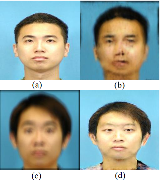
Figure 3: Translation results of Lee et al. (2018) for image de-blurring task. (a) real image. (b) blurred version of (a). (c) real blurred image. (d) deblurred version of (c). We can see that if adapting Lee et al. (2018) for image de-blurring task, the de-blurred images have different face contours from original ones, which means that the attribute extractor has not only learned blur distortion pattern but also recognized some content representations such as face contour as attribute. It might be attributed to the ambiguous and implicit disentanglement of content and style.

To alleviate this situation, we design an intra-domain supervision to constrain the disentangled representation learning and represent the essence of different domains. The main idea to achieve this is relatively simple: “Two images from the same domain exchange their style codes, the generated images should be consistent with themselves.” Different from style codes extracted from a single image $s_{i}\in\mathcal{S}_{i}$, these style codes extracted at domain level should be domain-specific and represent generalized domain style representations. For $n$ domains of datasets $\{\mathcal{D}_{1},\mathcal{D}_{2},\cdots,\mathcal{D}_{n}\}$, we have $n$ domains style representations $\{\mathcal{S}_{\mathcal{D}_{1}},\mathcal{S}_{\mathcal{D}_{2}},\cdots,\mathcal{S}_{\mathcal{D}_{n}}\}$. We can call this translation as intra-domain translation. As shown in Figure 2, intra-domain and inter-domain translation can be representation as

$$x_{1} = G_{1}(c,s_{1}), x_{2} = G_{2}(c,s_{2}),$$ (2)

$$x_{1\rightarrow 2} = G_{2}(c,s_{2}), x_{2\rightarrow 1} = G_{1}(c,s_{1}),$$

$$x_{1\rightarrow 1^{\prime}} = G_{1}(c,\mathcal{S}_{\mathcal{D}_{1}}), x_{1^{\prime}\rightarrow 1} = G_{1}(c,\mathcal{S}_{\mathcal{D}_{1}}).$$

The intra-domain translation aims to learn the essence style of a domain, which means the learned style representations of images from the same domain do not vary to an unreasonable degree. Specifically, all images converge to the “mean” style. After training on carefully selected images, this constraint helps the content and style encoders learn explicit disentangled representations during inter-domain translation. We can readily control its influence by changing the weight parameters.

3.3 Pre-training of domain style representation extractor

Different from many previous works regarding multiple domains as different sources of images, we treat each domain as explicit supervision. Similarly to Lin et al. (2019), we pre-train a domain feature representation extractor for each domain as explicit domain supervision.

For domain supervision, Lin et al. (2019) train a classifier that tries to correctly distinguish images of different domains. Then they regard the output of second-to-last layer of the classifier as the domain feature. Different from this ambiguous and implicit definition, we try to learn the domain feature representations by intra-domain translation.

Given images from $n$ different domains, we train a CNN network by switching style codes of images from the same domain. The goal of this CNN network, which we call domain representation extractor $E_{\mathcal{D}_{i}}^{s}$, is to learn domain-specific style representations $\mathcal{S}_{\mathcal{D}_{1}}$ for domain $\mathcal{D}_{i}$ and to correctly classify the domain of an image. Then this pre-trained model $E_{\mathcal{D}_{i}}^{s}$ is used as explicit domain supervision for inter-domain translation.

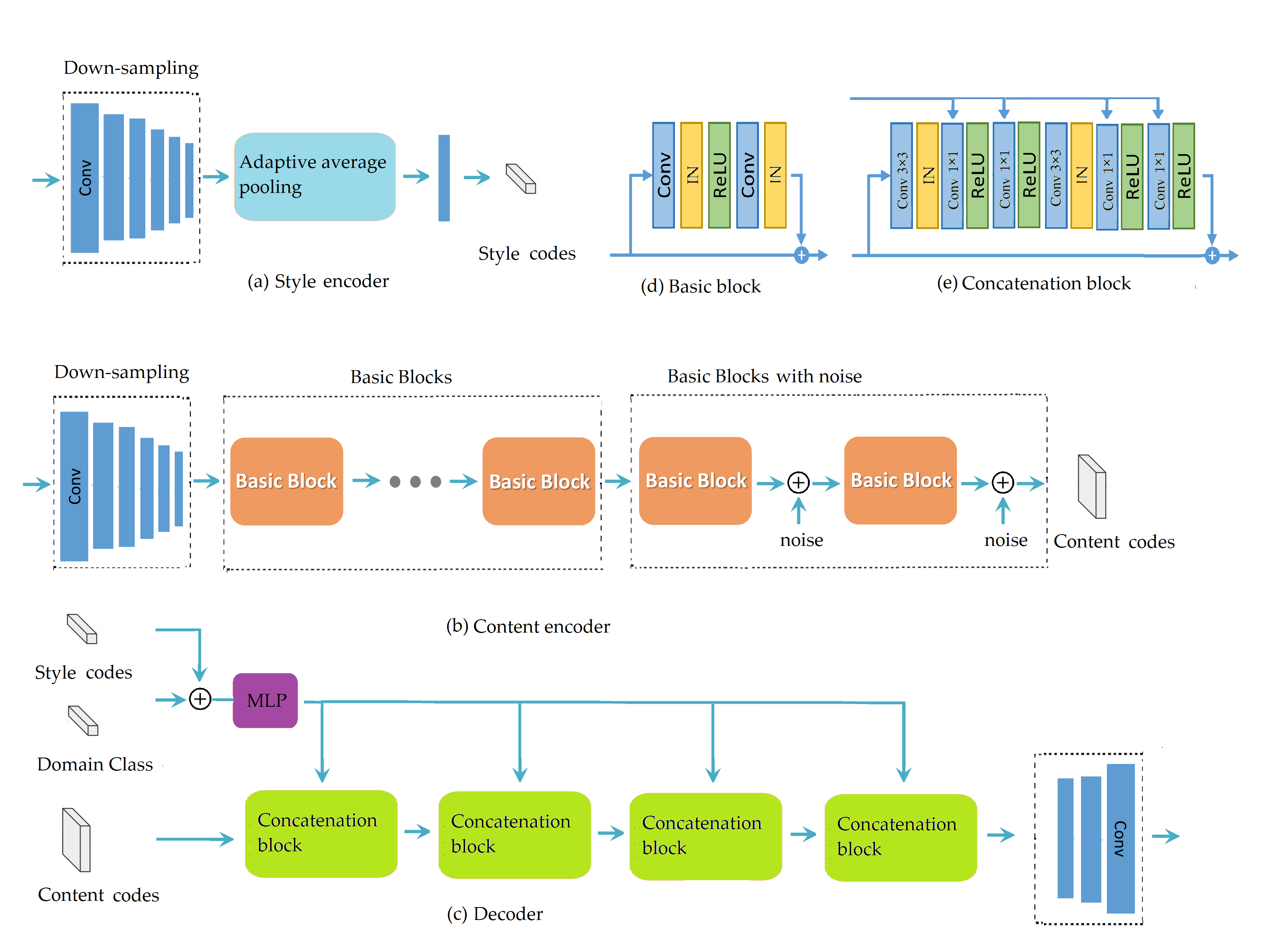
Figure 4: Network architecture. For more details, refer to Section 3.5.

3.4 Model

As aforementioned, the pipeline of our model is shown in Figure 1. Similar to other unsupervised image-to-image translation via disentangled representations (Liu et al., 2018; Lee et al., 2018; Huang et al., 2018), our model consists of a content encoder ${E}^{c}_{i}$ , style encoder ${E}^{s}_{i}$, decoder $G$ and discriminator $D_{i}$ for each domain $\mathcal{D}_{i}(i=1,2,\cdots,n)$. What’s more, in our experiment, we have the domain classifier $D_{cls}$ pre-trained together with the domain style representation extractor $E_{\mathcal{D}_{i}}^{s}$.

As shown, to achieve image translation between two domains $\{\mathcal{D}_{1},\mathcal{D}_{2}\}$, images $x_{1}$, $x_{2}$ from different domains are encoded as domain-invariant content representations $c_{1}=E_{1}^{c}\left(x_{1}\right)$, $c_{1}=E_{2}^{c}\left(x_{2}\right)$; and domain-specific style representations $s_{1}=E_{1}^{2}\left(x_{1}\right)$, $s_{2}=E_{s}^{2}\left(x_{2}\right)$. Then swap the style codes and use ${G}_{2}$ to produce the translated output image $x_{1\rightarrow 2}=G_{2}\left(c_{1},s_{2}\right)$.

3.5 Network architecture

Figure 4 shows the network architecture of our model. It consists of a content encoder, a style encoder and a decoder.

Content encoder.

The content encoder consists of several convolutional layers to down-sample the input images to get high-dimension features and several basic blocks for further processing. There are many choices for basic block such as residual block (He et al., 2016), residual dense block (Zhang et al., 2018b), residual in residual dense block (Wang et al., 2018b). Here we use the traditional residual block for simplicity and replace Batch Normalization (BN) (Ioffe and Szegedy, 2015) layer with Instance Normalization (IN) (Ulyanov et al., 2016b). For diversity, we add noise in the last two basic blocks as in Lee et al. (2018).

Style encoder.

The style encoder includes several strided convolutional layers, followed by an adaptive average pooling layer and a convolutional layer. We do not use IN layers in the style encoder, as IN removes the original feature mean and variance which represent important style information.

Decoder.

The decoder generates images from their content codes and style codes. For multi-domain translation, we also add domain class as input. Specifically, the domain class and style codes are concatenated by channel and then fed into a multi-layer perceptron (MLP). The the content codes and outputs generated by the MLP are further processed via several concatenation blocks. We equip the residual blocks with Adaptive Instance Normalization (AdaIN) (Huang and Belongie, 2017) layers whose parameters are dynamically generated by the MLP from the style codes (Huang and Belongie, 2017; Ghiasi et al., 2017).

$$\operatorname{AdaIN}(z,\gamma,\beta)=\gamma\left(\frac{z-\mu(z)}{\sigma(z)}\right)+\beta$$ (3)

Discriminator and domain classifier.

The architecture of discriminator is similar with Choi et al. (2018). The domain classifier is built on top of the discriminator, as shown in Figure 5. It consists of six convolution layers with kernel size $4\times 4$ and stride $2$, following two separated convolutional branches that are implemented for discriminative output and domain class.

Domain style representation extractor.

The domain style representation extractor shares the same architecture with style encoder. Specifically, it consists of one convolution layer with kernel size $4\times 4$ and stride $1$; six convolution layers with kernel size $4\times 4$, stride $2$ and ReLU followed by an adaptive average pooling layer and a convolutional layer with kernel size $1\times 1$, stride $1$.

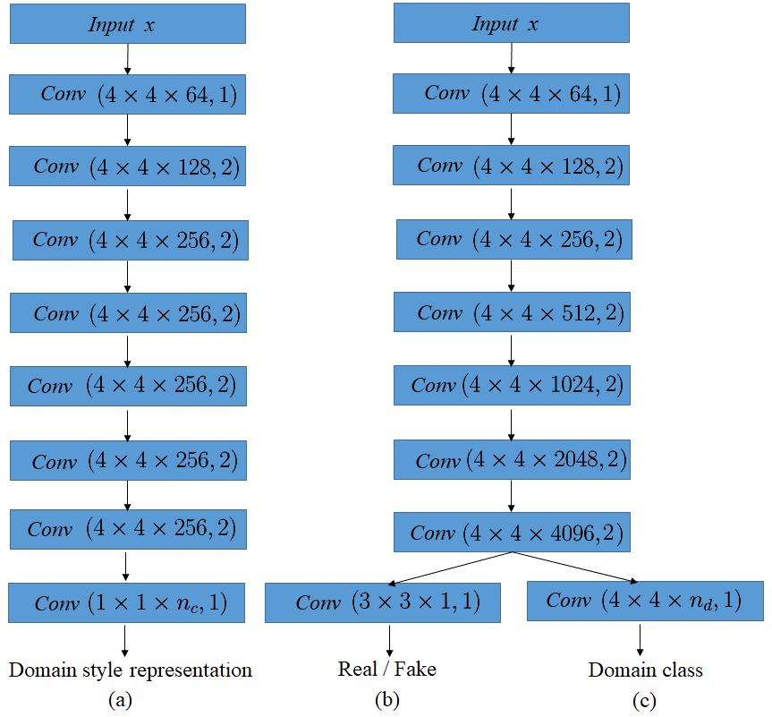
Figure 5: Discriminator and domain classifier.

3.6 Loss function

The loss functions are designed for unsupervised multi-domain multi-modal image-to-image translation. For unsupervised training, we adapt image reconstruction loss and latent reconstruction loss based on cycle consistent loss. We also add constraints to improve the representations of content and style codes by self-reconstruction loss. For multi-modality, we introduce a distribution matching loss to make the style codes extracted by content encoder close to a prior Gaussian distribution. By doing this, we are able to sample style codes from prior Gaussian distribution at testing phase. Since the sampled style codes are random and stochastic, the decoder can produce diverse samples sharing the same content. For simultaneous training of multiple different domains, we adapt a domain classification loss.

Self reconstruction loss.

Given an image from a certain domain, we should be able to reconstruct itself after encoding and decoding. Thus the self reconstruction loss $\mathcal{L}_{\mathrm{sr}}$ can be written as

$$\mathcal{L}_{\mathrm{sr}}^{x_{1}}=\mathbb{E}_{x_{1}\sim p\left(x_{1}\right)}\left[\left\|G_{1}\left(E_{1}^{c}\left(x_{1}\right),E_{1}^{s}\left(x_{1}\right)\right)-x_{1}\right\|_{1}\right].$$ (4)

Image reconstruction loss.

Given an image sampled from the data distribution, we should be able to reconstruct it after encoding and decoding. The image reconstruction loss $\mathcal{L}_{\mathrm{cc}}$ is adapted in two stages. In the pre-training of domain representations, we use image reconstruction loss to obtain a domain-specific style representation extractor $E_{\mathcal{D}_{i}}^{s}$ during the process of image reconstruction.

$$\mathcal{L}_{\mathrm{cc}}^{x}=\mathbb{E}_{x\sim p\left(x\right)}\left[\left\|G_{1}\left(E_{1}^{c}\left(x\right),E_{\mathcal{D}_{i}}^{s}\left(x^{\prime}\right)\right)-x\right\|_{1}\right],$$ (5)

where $x$ and $x^{\prime}$ are from the same domain.

In inter-domain translation, image reconstruction loss $\mathcal{L}_{\mathrm{cc}}$ is used for the style from a single image. The image reconstruction loss can be represented as:

$$\mathcal{L}_{\mathrm{cc}}^{x} = \mathbb{E}_{x,y}\left[\left\|G_{1}\left(E_{2}^{c}(y^{\prime}),E_{1}^{s}(x^{\prime})\right)-x\right\|_{1}\right],$$ (6)

$$\mathcal{L}_{\mathrm{cc}}^{y} = \mathbb{E}_{x,y}\left[\left\|G_{2}\left(E_{1}^{c}(x^{\prime}),E_{2}^{s}(y^{\prime})\right)-y\right\|_{1}\right],$$

where

$$x^{\prime}= G_{1}\left(E_{2}^{c}(y)\right),E_{1}^{s}(x)),$$ (7)

$$y^{\prime}= G_{2}\left(E_{1}^{c}(x)\right),E_{2}^{s}(y)).$$

Disentanglement constrained loss.

To utilize domain information and explicitly constrain the disentanglement, we propose the disentanglement loss. For style from domain style representation, the disentanglement constrained loss $\mathcal{L}_{\mathrm{dc}}$ can be represented as

$$\mathcal{L}_{\mathrm{dc}}^{x}=\mathbb{E}_{x,y}\left[\left\|y^{\prime}-y^{\prime\prime}\right\|_{1}\right],\\$$ (8)

where $y^{\prime\prime}=G_{2}\left(E_{2}^{c}(x),\mathcal{S}_{\mathcal{Y}}\right)$, $\mathcal{S}_{\mathcal{Y}}$ is extracted domain style.

Latent reconstruction loss.

Given a latent code (style and content) sampled from the latent distribution at translation time, we should be able to reconstruct it after decoding and encoding.

$$\mathcal{L}_{\mathrm{lr}}^{c_{1}} = \mathbb{E}_{c_{1}\sim p\left(c_{1}\right),s_{2}\sim q\left(s_{2}\right)}\left[\left\|E_{2}^{c}\left(G_{2}\left(c_{1},s_{2}\right)\right)-c_{1}\right\|_{1}\right],$$ (9)

$$\mathcal{L}_{\mathrm{lr}}^{s_{2}} = \mathbb{E}_{c_{1}\sim p\left(c_{1}\right),s_{2}\sim q\left(s_{2}\right)}\left[\left\|E_{2}^{s}\left(G_{2}\left(c_{1},s_{2}\right)\right)-s_{2}\right\|_{1}\right].$$

Distribution matching loss.

We adapt a distribution matching loss to make the style codes close to a prior Gaussian distribution. At testing phase, we are able to sample stochastically from prior Gaussian distribution and regard it as style code. As demonstrated in Section 2.5, the measure of distance between two distributions can be covariance, MMD or KL divergence. Instead of implementing KL divergence as in Huang et al. (2018) and Lee et al. (2018), here we choose the Maximum-Mean Discrepancy (MMD). We will illustrate the reasons in Section 4.7.

The distribution matching loss $\mathcal{L}_{\mathrm{dm}}$ described by MMD can be written as

$$\mathcal{L}_{\mathrm{dm}}=\mathbb{E}\left[D_{\mathrm{MMD}}\left(z|N(0,1)\right)\right],$$ (10)

where

$$D_{\mathrm{MMD}}(q|p) =\mathbb{E}_{p(z),p\left(z^{\prime}\right)}\left[k\left(z,z^{\prime}\right)\right]-2\mathbb{E}_{q(z),p\left(z^{\prime}\right)}\left[k\left(z,z^{\prime}\right)\right]$$ (11)

$$+\mathbb{E}_{q(z),q\left(z^{\prime}\right)}\left[k\left(z,z^{\prime}\right)\right]$$

$k(\cdot,\cdot)$ can be any positive definite kernel, such as Gaussian $k\left(z,z^{\prime}\right)=e^{-\frac{\left\|z-z^{\prime}\right\|^{2}}{2\sigma^{2}}}$.

Domain classification loss.

To achieve simultaneous training of multiple domains with a single model, we assign a unique class label for each domain as in Choi et al. (2018). While translating given input images $x_{1}$ with domain class $c_{1}$ to $x_{2}$ with $c_{2}$, the auxiliary domain classifier tries to distinguish images from different domains. The corresponding domain classification loss can be defined as

$$\mathcal{L}_{\mathrm{cls}}^{real}= \mathbb{E}_{x,c^{\prime}}\left[-\log D_{\mathrm{cls}}\left(c^{\prime}|x\right)\right],$$ (12)

$$\mathcal{L}_{\mathrm{cls}}^{fake}= \mathbb{E}_{x,c}\left[-\log D_{\mathrm{cls}}(c|G(x,c))\right],$$

where $D_{\mathrm{cls}}\left(c^{\prime}|x\right)$ represents a probability distribution over domain labels calculated by $D$. The goal of this term is that $D$ can correctly classify a real image $x$ to its original domain $c^{\prime}$ and $G$ tries to generate images that can be recognized as target domain $c$ by $D$.

This auxiliary domain classifier is build on top of discriminator $D$. In training phase, the domain classification loss of real images is used to optimize parameters of discriminator $D$ and the domain classification loss of fake images is used to optimize $G$.

In our experiment, the domain classifier $D_{cls}$ is pre-trained together with the domain style representation extractor $E_{\mathcal{D}_{i}}^{s}$.

Adversarial loss.

For high image quality, stable training and considerable diversity as discussed in Section 2.1, we use the least-squares GAN proposed by Mao et al. (2017). Thus $\mathcal{L}_{\mathrm{adv}}$ can be formulated as:

$$\min_{D_{1}}\mathcal{L}_{\mathrm{adv}}\left(D_{1}\right)= \frac{1}{2}\mathbb{E}_{\boldsymbol{x}\sim p{\mathrm{(}\boldsymbol{x})}}\left[\left(D_{1}(\boldsymbol{x})-b\right)^{2}\right]+$$ (13)

$$\frac{1}{2}\mathbb{E}_{\boldsymbol{z}\sim p_{\boldsymbol{z}}(\boldsymbol{z})}\left[\left(D_{1}\left(G_{1}(\boldsymbol{z})\right)-a\right)^{2}\right]$$

$$\min_{G_{1}}\mathcal{L}_{\mathrm{adv}}\left(G_{1}\right)= \frac{1}{2}\mathbb{E}_{\boldsymbol{z}\sim p_{z}(\boldsymbol{z})}\left[\left(D_{1}\left(G_{1}(\boldsymbol{z})\right)-c\right)^{2}\right].$$

Overall training loss.

The total training loss functions of the encoder $E$, decoder $G$ and discriminator $D$ are defined as follows:

$$\mathcal{L}_{\mathrm{E\circ G}}^{\mathrm{total}} = \mathcal{L}_{\mathrm{adv}}+\lambda_{\mathrm{sr}}\mathcal{L}_{\mathrm{sr}}+\lambda_{\mathrm{cc}}\mathcal{L}_{\mathrm{cc}}+\lambda_{\mathrm{dc}}\mathcal{L}_{\mathrm{dc}}$$ (14)

$$+ \lambda_{\mathrm{dm}}\mathcal{L}_{\mathrm{dm}}+\lambda_{\mathrm{lr}}\mathcal{L}_{\mathrm{lr}}+\lambda_{\mathrm{cls}}\mathcal{L}_{\mathrm{cls}}^{fake},$$

$$\mathcal{L}_{D}^{\mathrm{total}} = \mathcal{L}_{\mathrm{adv}}+\lambda_{\mathrm{cls}}\mathcal{L}_{\mathrm{cls}}^{real},$$ (15)

where hyper-parameters $\lambda_{sc}$, $\lambda_{cc}$, $\lambda_{dl}$, $\lambda_{dm}$, $\lambda_{lr}$ and $\lambda_{cls}$ are weights to control the importance of each term.

The overall process.

The overall process is summarized in Algorithm 1. The training process consists of two phase: the domain style representation extractor training and cross-domain translation training. Both phases share almost the same network architecture and loss functions except the following differences. Since we want to learn domain style representation from each domain and adapt it to cross-domain translation as domain supervision, we select images from the same domain and swap their style codes. Ideally, the style-exchanged images should be consisted with the original ones. Only one-step translation is required to get the domain style representation. So the loss function of the domain style representation extractor training can be defined as:

$$\mathcal{L}_{\mathrm{E\circ G}}^{\mathrm{total}} = \mathcal{L}_{\mathrm{adv}}+\lambda_{\mathrm{sr}}\mathcal{L}_{\mathrm{sr}}+\lambda_{\mathrm{dm}}\mathcal{L}_{\mathrm{dm}}+\lambda_{\mathrm{cls}}L_{\mathrm{cls}}^{fake},$$ (16)

$$\mathcal{L}_{D}^{\mathrm{total}} = \mathcal{L}_{\mathrm{adv}}+\lambda_{\mathrm{cls}}\mathcal{L}_{\mathrm{cls}}^{real},$$ (17)

where hyper-parameters $\lambda_{\mathrm{sc}}$, $\lambda_{\mathrm{dm}}$, $\lambda_{\mathrm{cls}}$ are weights to control the importance of each term.

Thus we get the domain style representation extractor $E_{\mathcal{D}_{i}}^{s}$. It mainly used in image reconstruction loss to constrain feature disentanglements.

1 Input: $N$ different domains $\mathcal{D}_{k}\ \forall k\in[N]$, batch size $N$, learning rate $\eta$;

Stage 1: domain style representation extractor training

2 Randomly initialize the parameters $\Theta_{E}$ of domain representation extractor $E_{\mathcal{D}}^{s}$;

3 Randomly select one domain $\mathcal{D}_{k}$, $k\in[N]$. Get a mini-batch of data $\mathcal{D}_{k}$ satisfying $D_{k}\subset\mathcal{D}_{k}$ and $\left|D_{k}\right|=K$;

4 Update the network as follows: $\Theta_{E\circ G}\leftarrow\Theta_{E\circ G}-\eta\nabla_{\Theta}\Theta_{E\circ G}\ell_{\mathrm{E\circ G}}^{\text{total }}\left(D_{\mathcal{S}}\right)$ $\Theta_{D}\leftarrow\Theta_{D}-\eta\nabla_{\Theta_{D}}\ell_{D}^{\mathrm{total}}\left(D_{\mathcal{S}}\right)$

5 where $\ell_{\mathrm{E\circ G}}^{\text{total }}\left(D_{\mathcal{S}}\right)$ and $\ell_{D}^{\text{total }}\left(D_{\mathcal{S}}\right)$ are defined in Eqn. 16 and Eqn. 17, respectively.

6 Repeat step $3$ and step $4$ until convergence.

Stage 2: cross-domain translation training

7 Randomly initialize the parameters $\Theta_{E\circ G}$ of content encoder $E^{c}$, style encoder $E^{s}$, decoder $G$ and parameters $\theta_{G}$ of discriminator $D$;

8 Randomly select two different domains $\mathcal{D}_{A},\mathcal{D}_{B},A,B\in[N]$ . For each selected domain $\mathcal{D}_{l}$ where $l\in\{A,B\}$, get a minibatch of data $D_{l}$ satisfying $D_{l}\subset\mathcal{D}_{l}$ and $\left|D_{l}\right|=K$.

9 if Training then

10       Update the parameters as follows: $\Theta_{E\circ G}\leftarrow\Theta_{E\circ G}-\eta\nabla_{\Theta}\Theta_{E\circ G}\ell_{\mathrm{E\circ G}}^{\text{total }}\left(D_{A}\right)$ $\Theta_{D}\leftarrow\Theta_{D}-\eta\nabla_{\Theta_{D}}\ell_{D}^{\mathrm{total}}\left(D_{A}\right)$

11where $\ell_{\mathrm{E\circ G}}^{\text{total }}\left(D_{A}\right)$ and $\ell_{D}^{\text{total }}\left(D_{A}\right)$ are defined in Eqn. 14 and Eqn. 15, respectively.

Repeat step $7$ and step $10$ until convergence.

Algorithm 1 Training process.

4 Experiment

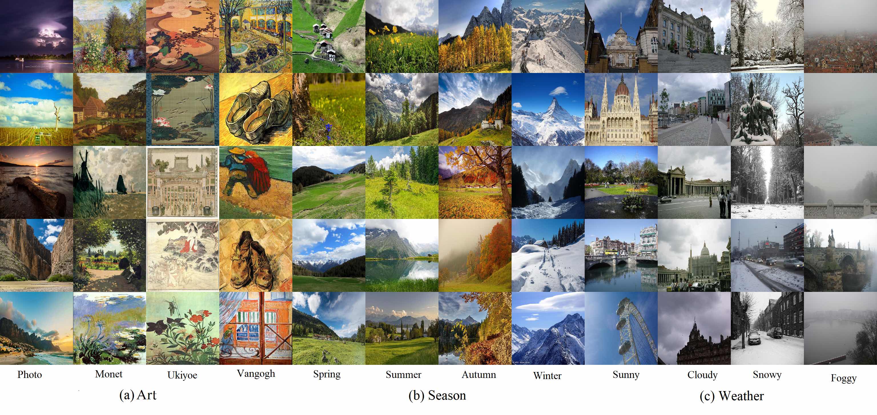
Figure 6: Samples from datasets. We mainly use three multi-domain datasets for experiments: Art, Season and Weather. Each contains four domains.

4.1 Experiment Settings

For training, we adapt Adam optimizer with a batch size $8$, a learning rate of $0.0001$ with exponential decay rates $\beta_{1}=0.5$, $\beta_{2}=0.999$. We resize all input images into $216\times 216$ in experiments. The hyper-parameters are set as $\lambda_{\mathrm{sr}}=10$, $\lambda_{\mathrm{cc}}=10$, $\lambda_{\mathrm{dm}}=0.01$, $\lambda_{\mathrm{lr}}=10$. And $\lambda_{\mathrm{cls}}$ of $G$ is $5.0$, $\lambda_{\mathrm{cls}}$ of $D$ is $1.0$. We don’t implement domain supervision if training data are paired.

4.2 Datasets

We use three multi-domain datasets for experiments: art, weather, season. Notice that all images in these datasets are not paired.

Art: This dataset contains four domains: real images, Monet, Ukiyo-e and Van Gogh. These art images can be download from Wikiart and the real photos are from Flickr with tags landscape and landscapephotography. We use the monet2photo, vangogh2photo, ukiyoe2photo and cezanne2photo datasets collected by Zhu et al. (2017a).

Weather: This dataset contains four domains: sunny, cloudy, snowy, and foggy, which is randomly selected from the Image2Weather (Chu et al., 2017).

Season: This dataset consists of approximately $6,000$ images of the Alps mountain range scraped from Flickr. The original dataset collected by Anoosheh et al. (2018) categorizes photos individually into four seasons based on the provided timestamp of when it was taken. But this lead to many misclassifications. We revise each category by deleting ambiguous images or removing misclassified images to the right category to make them more distinguishable.

Since Zhu et al. (2017b) need paired data for training, we evaluate multi-modality on edges $\rightarrow$ shoes and edges $\rightarrow$ handbags. The edges $\rightarrow$ shoes dataset contains 50k training images from UT Zappos50K dataset (Yu and Grauman, 2014). The edges $\rightarrow$ handbags dataset contains 137K Amazon Handbag images from Zhu et al. (2016). Edges are computed by HED edge detector (Xie and Tu, 2015) and post-processing. Both datasets can be downloaded at CycleGAN (Zhu et al., 2017a) website.

Samples from these three datasets are visually demonstrated in Figure 6 to describe their styles. And Table 2 describes domain information and corresponding number of training data.

Table 2: Features of each datasets.

Art	Num.	Weather	Num.	Season	Num.
Photos	2853	Sunny	70601	Spring	1382
Monet	1074	Cloudy	45662	Summer	1512
Van Gogh	401	Foggy	357	Autumn	1606
Ukiyo-e	1433	Snowy	1252	Winter	993

4.3 Baselines

We perform the evaluation on the following baseline approaches:

BicycleGAN. BicycleGAN (Zhu et al., 2017b) is the first image-to-image translation model that aims to generate continuous and multi-modal output images. However, it needs paired images for training.

DRIT (Lee et al., 2018) and MUNIT (Huang et al., 2018) propose to simultaneously generate diverse outputs given the same input image without requirement of pair supervision via disentangled representations. It’s designed for translation between two domains.

StarGAN. StarGAN (Choi et al., 2018) aim to handle scalability of unsurprised image-to-image translation problems. It uses one generator and discriminator in common for all domains by adding domain labels. The generator requires images and the desired domain label specifying the target domain as inputs, and the discriminator is trained to classify the domain labels of generated images and judge whether it’s real or fake. By doing this, it’s able to take any number of domains as input. However, the model was just applied on task of face attribute translation in original paper. It didn’t validate on datasets with various categories. Furthermore, it didn’t pay attention on the problem of multi-modality.

DosGAN. DosGAN (Lin et al., 2019) share the similar idea of (Choi et al., 2018) to achieve simultaneous training for multi-domains. It farther introduce the domain supervision, which uses domain-level information as supervision and pre-trains a classifier to predict which domain an image is from. The authors believe that the classifier should carry rich domain signal. Therefore, the output of the second-to-last layer of this classifier can be leveraged to extract the domain features of an image. Still, it follows the same drawback to diversity with Choi et al. (2018).

ComboGAN. Different from Choi et al. (2018) and Lin et al. (2019), Anoosheh et al. (2018) don’t use domain labels to achieve simultaneous training for multi-domains. Instead, it uses $n$ generators and discriminators for translations among $n$ domains. Specifically, it divides each generator network in half, labeling each one as encoders and decoders, respectively, and then assigns an encoder and decoder to each domain.

Since that those methods are designed for different purposes, we conduct comparisons on two criterions. For simultaneous training, we compare our approach with Choi et al. (2018), Lin et al. (2019) and Anoosheh et al. (2018). For multi-modality, we compare our method with Zhu et al. (2017b), Lee et al. (2018) and Huang et al. (2018).

Figure 7: Multi-domain multi-modal image translation results on Art. The Art dataset contains four domain: real image, Monet, Van Gogh and Ukiyoe. Better look by zooming in.

Figure 8: Multi-domain multi-modal translation result on Season. The Season dataset contains four domain: spring, summer, autumn and winter. Notice that all these image are generated via one training process. Better look by zooming in.

4.4 Evaluation Metrics

We use the Fr$\acute{e}$chet Inception distance and LPIPS Distance to evaluate the quality and diversity of the generated images.

LPIPS Distance. Similar to Zhu et al. (2017b), we use Learned Perceptual Image Patch Similarity (LPIPS) metric (Zhang et al., 2018a) to measure translation diversity. LPIPS Distance is calculated by a weighted $\mathcal{L}_{2}$ distance between deep features of randomly-sampled translation results from the same input. It has been shown to correlate well with human perceptual similarity.

FID score. Fr$\acute{e}$chet Inception distance (FID) (Heusel et al., 2017) is a measure of similarity between two datasets of images. It was shown to correlate well with human judgement of visual quality and is most often used to evaluate the quality of samples of Generative Adversarial Networks. FID is calculated by computing the Fr$\acute{e}$chet Inception distance between two Gaussians fitted to feature representations of the Inception network.

4.5 Qualitative evaluation

Figure 9: Results of StarGAN, DosGAN, ComboGAN and ours on Season dataset. Images in the first column are input images randomly selected from the four seasons. Following are results generated by ours, StarGAN, DosGAN and ComboGAN. For each method, the four columns are arranged successively as spring, summer, autumn and winter. Better look by zooming in.

We conduct comparisons on two criterions. For simultaneous training, we compare our approach with Choi et al. (2018), Lin et al. (2019) and Anoosheh et al. (2018) on season dataset. For multi-modality, we compare our method with Zhu et al. (2017b), Lee et al. (2018) and Huang et al. (2018) on edges $\rightarrow$ shoes and edges $\rightarrow$ handbags datasets. Qualitative comparison of simultaneous multi-domain translation with baselines on Season dataset are demonstrated in Figure 9. The results produced by Choi et al. (2018) all have obvious artifacts. Lin et al. (2019) generate fewer artifacts than Choi et al. (2018). However, the results are still unpleasing and lack diversity for different seasons. In most cases, the translated spring and summer images are almost indistinguishable. All four translated season images are even nearly the same in the last row of Lin et al. (2019). Anoosheh et al. (2018) generate better results in both realism and diversity than the aforementioned two methods. However, it needs $8$ generators and$4$ discriminators to achieve conversion of four seasons between any two.

Compared with baseline methods, our approach generates high-quality images which are more photo-realistic and diverse. The green blocks in Figure 9 represent real input images. Those real images can still be easily told apart from the generated ones translated by Anoosheh et al. (2018). In terms of realism,the real input images are indistinguishable from the four images generated by our method while in terms of diversity, the four season images can be easily classified into corresponding category. More results of our method on art, season and weather translation can be found in Figure 7, Figure 8 and Figure 10.

Figure 10 shows the results of our methods conducted on weather dataset. The images in the first row demonstrate that our method can handle images with complex and elaborate structures. The rest images show its potential capacities to the image defogging tasks.

Figure 11 shows the results of qualitative comparison on edges $\rightarrow$ shoes and edges $\rightarrow$ handbags.

Figure 10: Weather result. The images in the first row demonstrate that our method can handle images with complex and elaborate structures. The rest images show its potential capacities to the image defogging tasks. Better look by zooming in.

Figure 11: Qualitative comparison on edges $\rightarrow$ shoes and edges $\rightarrow$ handbags. The first column shows the input and ground truth image. Each following column shows three random possible outputs from corresponding method. Better look by zooming in.

4.6 Quantitative evaluation

We conduct the quantitative evaluation on the realism and diversity of season cross-domain translation (Anoosheh et al., 2018).

For realism, we conduct a user study using pairwise comparisons. Given a pair of images sampled from real images and translation outputs generated from different methods, users need to answer two questions: “Which image of this pair is more realistic?” and “Which season is this image?” They are given unlimited time to select their preferences. For each comparison, we randomly generate $100$ questions and each question is answered by $30$ different persons. Table 4 show the results of fooling rate and season classification accuracy. Anoosheh et al. (2018) get the highest fooling rate of $47.33\%$ and ours rank the second highest. Notice that Anoosheh et al. (2018) use several encoders and decoders to achieve this and our method only use one model. For season classification accuracy, since many images in Season dataset are too ambiguity to classify it into a certain season, the classification accuracy of the real images is like random guess, $48.9\%$. But the image-to-image translation methods tend to learn the general properties, the generated images are endowed with more distinguishable properties of certain season. Lin et al. (2019) and Anoosheh et al. (2018) get higher classification accuracy that real images, i.e., $54.2\%$ and $55.6\%$. And ours achieve the highest accuracy of $65.8\%$, which means the domain-specific styles are better captured by our proposed method. Figure 12 demonstrate the realism preference results. We conduct another user study to ask people to select a more realistic one between ours and Choi et al. (2018), Lin et al. (2019), Anoosheh et al. (2018), real images. The number indicates the percentage of preference on the pairwise comparisons. We use the season translation for this experiment.

For diversity, similar to Zhu et al. (2017b), we use the LPIPS metric to measure the similarity among images. Additionally, we implement FID to acquire perceptual scores. We compute the distance between $1000$ pairs of randomly sampled images translated from $100$ real images. As shown in Table 3, our method achieves the lowest FID scores, which means that our method produces the best results in both high-level similarity and perceptual judgement, and the highest LPIPS scores, which means the most diverse results.

As Zhu et al. (2017b) need paired data for training, we evaluate multi-modality on edges $\rightarrow$ shoes and edges $\rightarrow$ handbags. We use the LPIPS and FID metric to compare our method with the existing state-of-the-art method, i.e., Zhu et al. (2017b); Lee et al. (2018); Huang et al. (2018). As shown in Table 5, our method outperforms the supervised method (Zhu et al., 2017b) and produce comparable results with other unsupervised methods (Zhu et al., 2017b; Lee et al., 2018; Huang et al., 2018).

Table 3: Perfomance as the LPIPS and FID on the Season dataset. The best and second best results are highlighted in each column. For details refer to Section 4.6.

Method	LPIPS	FID
Choi et al. (2018)	0.4273	221.7
Lin et al. (2019)	0.2503	145.3
Anoosheh et al. (2018)	0.4349	109.99
Ours	0.4810	73.47

Table 4: Perfomance as the Fooling Rate and Season Classification Accuracy on the Season dataset. We conduct the user study to select results that are more realistic through pairwise comparisons and distinguish which season of an image is. The number indicates the percentage of preference on that comparison pair. The best and second best results are highlighted in each column. For details refer to Section 4.6.

Method	Fooling Rate	Accuracy
Real photos	-	48.9%
Choi et al. (2018)	5.3%	41.3%
Lin et al. (2019)	27.2%	54.2%
Anoosheh et al. (2018)	47.33%	55.6%
Ours	37.8%	65.8%

Table 5: Diversity. We use the LPIPS and FID metric to measure the diversity of generated images on the edges $\rightarrow$ shoes and edges $\rightarrow$ handbags. The best and second best results are highlighted in each column.

Method	edges $\rightarrow$ shoes		edges $\rightarrow$ handbags
	LPIPS	FID	LPIPS	FID
Zhu et al. (2017b)	0.2443	115.87	0.3180	184.56
Lee et al. (2018)	0.2631	62.67	0.3760	90.89
Huang et al. (2018)	0.2652	65.87	0.3820	91.43
Ours	0.2639	64.46	0.3759	89.19

Figure 12: Realism preference results. We conduct a user study to ask people to select a more realistic one between ours and Choi et al. (2018), Lin et al. (2019), Anoosheh et al. (2018). The number indicates the percentage of preference on the pairwise comparisons. We use the season translation for this experiment.

4.7 Ablation study

The effect of domain supervision.

As illustrated in Section 3.2, the de-blurred images of Lee et al. (2018) have different face contour with original ones, which means that the attribute extractor has not only learned blur distortion pattern but also recognize some content representations such as face contour as attribute. It might be caused by the ambiguous and implicit disentanglement of content and style. Thus we introduce explicit domain-constraint for disentanglement of content and style to better utilize domain information and explicitly constrain the disentanglement learning.

Figure 13 shows the style-swapped reconstruction results of intra-domain translation. It only shows that the pre-trained model could reconstruct style-swapped images from the same domain but fail to proof the domain supervision help the explicit disentanglement learning of content and style. To further validate the effectiveness of domain supervision, we adapt our method for image de-blurring task, and compare with the results of Lee et al. (2018) in Figure 3. The blurred images are generated using the same method as in Yu et al. (2018c) and CUFS dataset (Wang and Tang, 2009). The results of image de-blurring after adding proposed disentanglement loss are shown in Figure 14. Compared with Figure 3, the generated image are consistent with the original except the blur distortion are removed.

Figure 13: Results of intra-domain supervision. Better look by zooming in.

Figure 14: Results of adapting our method for image de-blurring. Better look by zooming in.

Furthermore, we also found that perceptual loss (Johnson et al., 2016) can achieve similar disentangled constraint. The perceptual loss is based on perceptual similarity, which is often computed as the distance of two activated features in a pre-trained deep neural network between the output and the reference image:

$$\mathcal{L}_{\text{percep}}=\mathbb{E}\left[\sum_{i}\frac{1}{N_{i}}\left\|\phi_{i}\left(\mathrm{I_{gt}}\right)-\phi_{i}(\mathrm{I_{pred}})\right\|_{1}\right],$$ (18)

where $\phi_{i}$ donates the feature maps of the pre-trained VGG-19 network.

The perceptual loss and disentanglement restrained loss constrain the learning of disentangled representations in different aspects. The former, which is image-level, forces the generated images sharing the same content with the input ones. The latter, which is collection-level, restrains the style encoder from learning any content of images.

The measure of distributions.

Many criteria can be used to estimate the distance between distributions. Kullback-Leibler (KL) divergence may be the most widely used in practice:

$$L_{\mathrm{dm}}=\mathbb{E}\left[D_{\mathrm{KL}}\left(\left(z\right)|N(0,1)\right)\right],$$ (19)

where $D_{\mathrm{KL}}(p|q)=-\int p(z)\log\frac{p(z)}{q(z)}\mathrm{d}z$.

However, researchers have noticed that KL divergence might be too restrictive (Bowman et al., 2015; Sønderby et al., 2016; Chen et al., 2016b; Bińkowski et al., 2018). Sometimes it failed to learn any meaningful latent representation. Several methods (Bowman et al., 2015; Sønderby et al., 2016; Chen et al., 2016b) try to alleviate this problem, but do not completely solve the issue. Borgwardt et al. (2006) propose the Maximum Mean Discrepancy (MMD) as a relevant criterion for comparing distributions based on the Reproducing Kernel Hilbert Space (RKHS). It’s a framework to quantify the distance of two c by calculating all of their moments. It can be efficiently adapted using kernel trick.

$$D_{\mathrm{MMD}}(q\|p) =\mathbb{E}_{p(z),p\left(z^{\prime}\right)}\left[k\left(z,z^{\prime}\right)\right]-2\mathbb{E}_{q(z),p\left(z^{\prime}\right)}\left[k\left(z,z^{\prime}\right)\right]$$ (20)

$$+\mathbb{E}_{q(z),q\left(z^{\prime}\right)}\left[k\left(z,z^{\prime}\right)\right],$$

where $k(\cdot,\cdot)$ can be any positive definite kernel, such as Gaussian $k\left(z,z^{\prime}\right)=e^{-\frac{\left\|z-z^{\prime}\right\|^{2}}{2\sigma^{2}}}$. Therefore, the distance between distributions of two samples can be well-estimated by the distance between the means of the two samples mapped into a RKHS.

To make this more intuitive, we conduct experiment on MNIST dataset (LeCun et al., 1998). For visualization, we make the latent code two dimensions. It can be seen in Figure 15 that with KL $q_{\phi}(z)$, the distribution matches the prior Gaussian distribution $p(z)$ poorly, while with MMD $q_{\phi}(z)$ matches significantly better. And results in Table 6 also demonstrate that MMD helps better reconstruction than KL.

Table 6: Feature visualization.

Method	Reconstruction loss	Log likelihood
KL	0.04367	82.75
MMD	0.03605	80.76

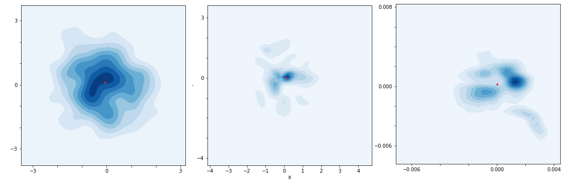
Figure 15: Comparing the prior Gaussian distribution $p(z)$, MMD $q_{\phi}(z)$ and KL $q_{\phi}(z)$. The red dots represent $(0,0)$. It clearly demonstrates that with KL $q_{\phi}(z)$, the distribution matches the prior Gaussian distribution $p(z)$ poorly, while with MMD $q_{\phi}(z)$ matches significantly better.

5 Conclusion

In this paper, we propose a unified framework for learning to generate diverse outputs with unpaired training data and allow simultaneous training of multiple datasets with different domains by a single network. Furthermore, we also investigate how to better extract domain supervision information so as to better utilize domain information and explicitly constrain the disentanglement. Qualitative and quantitative experiments on different datasets show that the proposed method outperforms the state-of-the-art methods.

6 Appendix

In this appendix, we show some additional cross-domain translation results of art in Figure 16, season in Figure 17 and weather in Figure 18.

Figure 16: Art result. Better look by zooming in.

Figure 17: Season result. Better look by zooming in.

Figure 18: Weather result. Better look by zooming in.

References

- Anoosheh et al. (2018) Anoosheh A, Agustsson E, Timofte R, Van Gool L (2018) Combogan: Unrestrained scalability for image domain translation. In: Proceedings of the IEEE Conference on Computer Vision and Pattern Recognition Workshops, pp 783–790
- Arjovsky et al. (2017) Arjovsky M, Chintala S, Bottou L (2017) Wasserstein generative adversarial networks. In: International Conference on Machine Learning, pp 214–223
- Berthelot et al. (2017) Berthelot D, Schumm T, Metz L (2017) Began: Boundary equilibrium generative adversarial networks. arXiv preprint arXiv:170310717
- Bińkowski et al. (2018) Bińkowski M, Sutherland DJ, Arbel M, Gretton A (2018) Demystifying mmd gans. arXiv preprint arXiv:180101401
- Borgwardt et al. (2006) Borgwardt KM, Gretton A, Rasch MJ, Kriegel HP, Schölkopf B, Smola AJ (2006) Integrating structured biological data by kernel maximum mean discrepancy. Bioinformatics 22(14):e49–e57
- Bousmalis et al. (2016) Bousmalis K, Trigeorgis G, Silberman N, Krishnan D, Erhan D (2016) Domain separation networks. In: Advances in Neural Information Processing Systems, pp 343–351
- Bousmalis et al. (2017) Bousmalis K, Silberman N, Dohan D, Erhan D, Krishnan D (2017) Unsupervised pixel-level domain adaptation with generative adversarial networks. In: Proceedings of the IEEE conference on computer vision and pattern recognition, pp 3722–3731
- Bowman et al. (2015) Bowman SR, Vilnis L, Vinyals O, Dai AM, Jozefowicz R, Bengio S (2015) Generating sentences from a continuous space. arXiv preprint arXiv:151106349
- Chen and Schmidt (2016) Chen TQ, Schmidt M (2016) Fast patch-based style transfer of arbitrary style. arXiv preprint arXiv:161204337
- Chen et al. (2016a) Chen X, Duan Y, Houthooft R, Schulman J, Sutskever I, Abbeel P (2016a) Infogan: Interpretable representation learning by information maximizing generative adversarial nets. In: Advances in Neural Information Processing Systems 29, 2016, pp 2172–2180
- Chen et al. (2016b) Chen X, Kingma DP, Salimans T, Duan Y, Dhariwal P, Schulman J, Sutskever I, Abbeel P (2016b) Variational lossy autoencoder. arXiv preprint arXiv:161102731
- Choi et al. (2018) Choi Y, Choi M, Kim M, Ha J, Kim S, Choo J (2018) Stargan: Unified generative adversarial networks for multi-domain image-to-image translation. In: 2018 IEEE Conference on Computer Vision and Pattern Recognition, CVPR 2018, pp 8789–8797
- Chu et al. (2017) Chu WT, Zheng XY, Ding DS (2017) Camera as weather sensor: Estimating weather information from single images. Journal of Visual Communication and Image Representation 46:233–249
- Denton et al. (2017) Denton EL, et al. (2017) Unsupervised learning of disentangled representations from video. In: Advances in neural information processing systems, pp 4414–4423
- Ganin and Lempitsky (2014) Ganin Y, Lempitsky V (2014) Unsupervised domain adaptation by backpropagation. arXiv preprint arXiv:14097495
- Ganin et al. (2016) Ganin Y, Ustinova E, Ajakan H, Germain P, Larochelle H, Laviolette F, Marchand M, Lempitsky V (2016) Domain-adversarial training of neural networks. The Journal of Machine Learning Research 17(1):2096–2030
- Gatys et al. (2016) Gatys LA, Ecker AS, Bethge M (2016) Image style transfer using convolutional neural networks. In: IEEE Conference on Computer Vision and Pattern Recognition, pp 2414–2423
- Ghiasi et al. (2017) Ghiasi G, Lee H, Kudlur M, Dumoulin V, Shlens J (2017) Exploring the structure of a real-time, arbitrary neural artistic stylization network. arXiv preprint arXiv:170506830
- Goodfellow et al. (2014) Goodfellow IJ, Pouget-Abadie J, Mirza M, Xu B, Warde-Farley D, Ozair S, Courville A, Bengio Y (2014) Generative adversarial nets. In: International Conference on Neural Information Processing Systems, pp 2672–2680
- Gulrajani et al. (2017) Gulrajani I, Ahmed F, Arjovsky M, Dumoulin V, Courville AC (2017) Improved training of wasserstein gans. In: Advances in Neural Information Processing Systems 30, 2017, pp 5769–5779
- He et al. (2016) He K, Zhang X, Ren S, Sun J (2016) Deep residual learning for image recognition. In: Computer Vision and Pattern Recognition, pp 770–778
- Heusel et al. (2017) Heusel M, Ramsauer H, Unterthiner T, Nessler B, Hochreiter S (2017) Gans trained by a two time-scale update rule converge to a local nash equilibrium. In: Advances in Neural Information Processing Systems, pp 6626–6637
- Huang and Belongie (2017) Huang X, Belongie S (2017) Arbitrary style transfer in real-time with adaptive instance normalization. In: Proceedings of the IEEE International Conference on Computer Vision, pp 1501–1510
- Huang et al. (2018) Huang X, Liu M, Belongie SJ, Kautz J (2018) Multimodal unsupervised image-to-image translation. In: Computer Vision - ECCV 2018 - 15th European Conference, Proceedings, Part III, pp 179–196
- Ioffe and Szegedy (2015) Ioffe S, Szegedy C (2015) Batch normalization: Accelerating deep network training by reducing internal covariate shift. arXiv preprint arXiv:150203167
- Isola et al. (2017) Isola P, Zhu J, Zhou T, Efros AA (2017) Image-to-image translation with conditional adversarial networks. In: 2017 IEEE Conference on Computer Vision and Pattern Recognition, CVPR 2017, pp 5967–5976
- Johnson et al. (2016) Johnson J, Alahi A, Li FF (2016) Perceptual losses for real-time style transfer and super-resolution. In: European Conference on Computer Vision, pp 694–711
- Kim et al. (2017) Kim T, Cha M, Kim H, Lee JK, Kim J (2017) Learning to discover cross-domain relations with generative adversarial networks. In: Proceedings of the 34th International Conference on Machine Learning-Volume 70, pp 1857–1865
- Kullback and Leibler (1951) Kullback S, Leibler RA (1951) On information and sufficiency. The annals of mathematical statistics 22(1):79–86
- LeCun et al. (1998) LeCun Y, Bottou L, Bengio Y, Haffner P, et al. (1998) Gradient-based learning applied to document recognition. Proceedings of the IEEE 86(11):2278–2324
- Ledig et al. (2017) Ledig C, Theis L, Huszar F, Caballero J, Cunningham A, Acosta A, Aitken AP, Tejani A, Totz J, Wang Z, Shi W (2017) Photo-realistic single image super-resolution using a generative adversarial network. In: 2017 IEEE Conference on Computer Vision and Pattern Recognition, CVPR 2017, pp 105–114
- Lee et al. (2018) Lee H, Tseng H, Huang J, Singh M, Yang M (2018) Diverse image-to-image translation via disentangled representations. In: Computer Vision - ECCV 2018 - 15th European Conference, Proceedings, Part I, pp 36–52
- Li and Wand (2016) Li C, Wand M (2016) Precomputed real-time texture synthesis with markovian generative adversarial networks. In: European Conference on Computer Vision, Springer, pp 702–716
- Lin et al. (2019) Lin J, Liu S, Xia Y, Zhao S, Qin T, Chen Z (2019) Unpaired image-to-image translation with domain supervision. arXiv preprint arXiv:190203782
- Liu et al. (2018) Liu AH, Liu Y, Yeh Y, Wang YF (2018) A unified feature disentangler for multi-domain image translation and manipulation. In: Advances in Neural Information Processing Systems 31, NeurIPS 2018, pp 2595–2604
- Liu et al. (2017) Liu M, Breuel T, Kautz J (2017) Unsupervised image-to-image translation networks. In: Advances in Neural Information Processing Systems 30: Annual Conference on Neural Information Processing Systems 2017, 4-9 December 2017, Long Beach, CA, USA, pp 700–708
- Long et al. (2014) Long M, Wang J, Ding G, Sun J, Yu PS (2014) Transfer joint matching for unsupervised domain adaptation. In: Proceedings of the IEEE conference on computer vision and pattern recognition, pp 1410–1417
- Long et al. (2015) Long M, Cao Y, Wang J, Jordan MI (2015) Learning transferable features with deep adaptation networks. arXiv preprint arXiv:150202791
- Lu et al. (2019) Lu B, Chen JC, Chellappa R (2019) Unsupervised domain-specific deblurring via disentangled representations. arXiv preprint arXiv:190301594
- Mao et al. (2017) Mao X, Li Q, Xie H, Lau RY, Wang Z, Paul Smolley S (2017) Least squares generative adversarial networks. In: Proceedings of the IEEE International Conference on Computer Vision, pp 2794–2802
- Nazeri et al. (2019) Nazeri K, Ng E, Joseph T, Qureshi FZ, Ebrahimi M (2019) Edgeconnect: Generative image inpainting with adversarial edge learning. CoRR abs/1901.00212
- Sønderby et al. (2016) Sønderby CK, Raiko T, Maaløe L, Sønderby SK, Winther O (2016) Ladder variational autoencoders. In: Advances in neural information processing systems, pp 3738–3746
- Sun and Saenko (2016) Sun B, Saenko K (2016) Deep coral: Correlation alignment for deep domain adaptation. In: European Conference on Computer Vision, Springer, pp 443–450
- Tsai et al. (2018) Tsai YH, Hung WC, Schulter S, Sohn K, Yang MH, Chandraker M (2018) Learning to adapt structured output space for semantic segmentation. In: Proceedings of the IEEE Conference on Computer Vision and Pattern Recognition, pp 7472–7481
- Tzeng et al. (2017) Tzeng E, Hoffman J, Saenko K, Darrell T (2017) Adversarial discriminative domain adaptation. In: Proceedings of the IEEE Conference on Computer Vision and Pattern Recognition, pp 7167–7176
- Ulyanov et al. (2016a) Ulyanov D, Lebedev V, Vedaldi A, Lempitsky VS (2016a) Texture networks: Feed-forward synthesis of textures and stylized images. In: Proceedings of the 33nd International Conference on Machine Learning, ICML 2016, pp 1349–1357
- Ulyanov et al. (2016b) Ulyanov D, Vedaldi A, Lempitsky V (2016b) Instance normalization: The missing ingredient for fast stylization. arXiv preprint arXiv:160708022
- Ulyanov et al. (2017) Ulyanov D, Vedaldi A, Lempitsky V (2017) Improved texture networks: Maximizing quality and diversity in feed-forward stylization and texture synthesis. In: Proceedings of the IEEE Conference on Computer Vision and Pattern Recognition, pp 6924–6932
- Wang et al. (2018a) Wang T, Liu M, Zhu J, Tao A, Kautz J, Catanzaro B (2018a) High-resolution image synthesis and semantic manipulation with conditional gans. In: 2018 IEEE Conference on Computer Vision and Pattern Recognition, CVPR 2018, pp 8798–8807
- Wang and Tang (2009) Wang X, Tang X (2009) Face photo-sketch synthesis and recognition. IEEE Trans Pattern Anal Mach Intell 31(11):1955–1967
- Wang et al. (2018b) Wang X, Yu K, Wu S, Gu J, Liu Y, Dong C, Qiao Y, Loy CC (2018b) ESRGAN: enhanced super-resolution generative adversarial networks. In: Computer Vision - ECCV 2018 Workshops, Proceedings, Part V, pp 63–79
- Xiao et al. (2018) Xiao T, Hong J, Ma J (2018) Elegant: Exchanging latent encodings with gan for transferring multiple face attributes. In: Proceedings of the European Conference on Computer Vision (ECCV), pp 172–187
- Xie and Tu (2015) Xie S, Tu Z (2015) Holistically-nested edge detection. In: Proceedings of IEEE International Conference on Computer Vision, pp 1395–1403
- Yi et al. (2017) Yi Z, Zhang H, Tan P, Gong M (2017) Dualgan: Unsupervised dual learning for image-to-image translation. In: Proceedings of the IEEE International Conference on Computer Vision, pp 2849–2857
- Yu and Grauman (2014) Yu A, Grauman K (2014) Fine-grained visual comparisons with local learning. In: Proceedings of IEEE International Conference on Computer Vision, pp 192–199
- Yu et al. (2018a) Yu J, Lin Z, Yang J, Shen X, Lu X, Huang TS (2018a) Free-form image inpainting with gated convolution. arXiv preprint arXiv:180603589
- Yu et al. (2018b) Yu J, Lin Z, Yang J, Shen X, Lu X, Huang TS (2018b) Generative image inpainting with contextual attention. arXiv preprint arXiv:180107892
- Yu et al. (2018c) Yu K, Dong C, Lin L, Loy CC (2018c) Crafting a toolchain for image restoration by deep reinforcement learning. In: Proceedings of IEEE Conference on Computer Vision and Pattern Recognition, pp 2443–2452
- Zellinger et al. (2017) Zellinger W, Grubinger T, Lughofer E, Natschläger T, Saminger-Platz S (2017) Central moment discrepancy (cmd) for domain-invariant representation learning. arXiv preprint arXiv:170208811
- Zhang et al. (2018a) Zhang R, Isola P, Efros AA, Shechtman E, Wang O (2018a) The unreasonable effectiveness of deep features as a perceptual metric. In: Proceedings of the IEEE Conference on Computer Vision and Pattern Recognition, pp 586–595
- Zhang et al. (2018b) Zhang Y, Tian Y, Kong Y, Zhong B, Fu Y (2018b) Residual dense network for image super-resolution. In: Proceedings of the IEEE Conference on Computer Vision and Pattern Recognition, pp 2472–2481
- Zhu et al. (2016) Zhu J, Krähenbühl P, Shechtman E, Efros AA (2016) Generative visual manipulation on the natural image manifold. In: Computer Vision - ECCV 2016, Proceedings, Part V, pp 597–613
- Zhu et al. (2017a) Zhu J, Park T, Isola P, Efros AA (2017a) Unpaired image-to-image translation using cycle-consistent adversarial networks. In: IEEE International Conference on Computer Vision, ICCV 2017, pp 2242–2251
- Zhu et al. (2017b) Zhu J, Zhang R, Pathak D, Darrell T, Efros AA, Wang O, Shechtman E (2017b) Toward multimodal image-to-image translation. In: Advances in Neural Information Processing Systems 30, 2017, pp 465–476