BIMC: The Bayesian Inverse Monte Carlo method for goal-oriented uncertainty quantification. Part I.

Abstract

We consider the problem of estimating rare event probabilities, focusing on systems whose evolution is governed by differential equations with uncertain input parameters. If the system dynamics is expensive to compute, standard sampling algorithms such as the Monte Carlo method may require infeasible running times to accurately evaluate these probabilities. We propose an importance sampling scheme (which we call “BIMC”) that relies on solving an auxiliary, “fictitious” Bayesian inverse problem. The solution of the inverse problem yields a posterior PDF, a local Gaussian approximation to which serves as the importance sampling density. We apply BIMC to several problems and demonstrate that it can lead to computational savings of several orders of magnitude over the Monte Carlo method. We delineate conditions under which BIMC is optimal, as well as conditions when it can fail to yield an effective IS density.

65C05, 62F15, 62P30

1 Introduction

We consider the following goal-oriented uncertainty quantification (UQ) problem. Let $f(\bm{x}):\mathbb{R}^{m}\rightarrow\mathbb{R}$ be a smooth nonlinear operator, and $p(\bm{x})$ a given probability density function (PDF) for $\bm{x}$. Given a target interval $\mathbb{Y}\subset\mathbb{R}$, our goal is to compute $\mu=\mathbb{P}(f(\bm{x})\in\mathbb{Y})$. Equivalently, $\mu$ is the expectation under $p(\bm{x})$ of the indicator function $\bm{\mathrm{1}}_{\mathbb{Y}}(f(\bm{x}))$. We focus on the case when $\mu\ll 1$, i.e., the event $f(\bm{x})\in\mathbb{Y}$ is rare.

In our context, $f(\bm{x})$ is a map from some random finite dimensional parameter space to a quantity-of-interest (QoI). Such parameter-to-QoI maps are often a composition of the solution of a differential equation for a state variable, and an operator that extracts the QoI from the state. The parameters $\bm{x}$ represent uncertain parameters in the physical model. This uncertainty can arise from a variety of sources, such as lack of knowledge, measurement errors, or noise. Here, we assume that the uncertainty is described by a known PDF, $p(\bm{x})$. A Monte Carlo (MC) method can be used to compute $\mu$ by sampling $\bm{x}$ from $p(\bm{x})$ and then checking whether $f(\bm{x})\in\mathbb{Y}$. But such an approach can be prohibitively expensive if the operator $f$ is expensive to evaluate, especially when $\mu\ll 1$.

Summary of the methodology

We propose a variance reduction scheme based on importance sampling (IS). In IS, samples are drawn from a new distribution, say $q(\bm{x})$, in order to increase the occurrences of the rare event. We construct our IS density as follows. We begin by setting up an auxiliary inverse problem. First we select a $y\in\mathbb{Y}$, and then we find $\bm{x}$ such that $f(\bm{x})\approx y$. This is an ill-posed or inverse problem since given a scalar $y$ we want to reconstruct the vector $\bm{x}$. A simple counting argument shows that this is impossible unless we use some kind of regularization. To address this ill-posedness we adopt a Bayesian perspective, that is, the solution of the inverse problem is not a specific point estimate $\bm{x}$ but a “posterior distribution”, $p(\bm{x}|y)$, a PDF on the parameters $\bm{x}$ conditioned on $y$. We will use a Gaussian approximation of this posterior around the Maximum A Posteriori (MAP) point as the importance sampling distribution. The mean of the approximating Gaussian is the MAP point itself, and its covariance is the inverse of the Gauss-Newton Hessian, $\mathbf{H}_{\mathrm{GN}}^{-1}$, of $-\log(p(\bm{x}|y))$ at the MAP point.

Contributions

In summary, our contributions are the following.

• We introduce the concept of solving inverse problems for forward uncertainty quantification.

• To our knowledge, this is the first algorithm that exploits derivatives of the forward operator $f$ to arrive at an IS density for simulating rare events.

• We offer a thorough theoretical analysis of the affine-Gaussian inverse problem. This analysis establishes conditions for optimality of our algorithm, as well as guides the tuning of various algorithmic “knobs”.

• We apply our methodology to several real and synthetic problems and demonstrate orders-of-magnitude speedup over a vanilla MC implementation.

Limitations

• The success of our algorithms depends strongly upon the quality (both in terms of accuracy and speed) of the inverse problem solution. When the operator $f$ involves differential equations, efficiently solving the inverse problem requires adjoint operators and perhaps sophisticated PDE-constrained optimization solvers and preconditioners.

• Our methodology has several failure mechanisms. These are described in detail in Figure 6. In light of these failure mechanisms, the question of a priori assessing the applicability of BIMC to a given problem (i.e., a given combination of $f(\bm{x})$, $p(\bm{x})$, and $\mathbb{Y}$) has also been left unexplored.

Related work

The literature on goal-oriented techniques, importance sampling, rare-event probability estimation, and Bayesian inference is quite extensive. Here, we review work that is most relevant.

Goal-oriented methods

The idea of goal-oriented techniques for UQ isn’t new (see [16, 17, 28]). However, most of these works focus on dimensionality reduction, and not rare events. Also pertinent is the measure-theoretic approach to inverse problems [5, 7].

Rare-event probability estimation

A large body of work on rare events has been motivated by the problem of assessing the reliability of systems. In such problems, the task is to compute the probability of failure of a system, which occurs when $f(\bm{x})<0$ (or in our framework, when $\mathbb{Y}=(-\infty,0)$).

Analytical approaches to approximate this failure probability include the First and Second Order Reliability Methods (see [23] for a review). These methods are based on approximating $f$ with a truncated Taylor series expansion around a “design” point. A drawback of these methods is that they have no means of estimating the error in the computed failure probability. We would like to note that the concept of “design” points here is similar to the MAP point in our algorithm, but they are not exactly identical. The design point, say $\bm{x}^{*}$, is always constrained to satisfy $f(\bm{x}^{*})=0$. That is, it lies at the edge of the pre-image $f^{-1}(\mathbb{Y})$. The MAP point, on the other hand, is expected to lie in the interior of the region $f^{-1}(\mathbb{Y})$. Moreover, the fact that $\bm{x}_{\mathrm{MAP}}$ lies in the interior of $f^{-1}(\mathbb{Y})$ is accounted for, and in fact, exploited, when we choose tunable parameters of our algorithm.

Statistical approaches to evaluate the failure probability have received considerable attention (see [26] for a review). As opposed to analytical methods, these methods have well-understood convergence properties, and they come with a natural error estimate. In this context, a simple Monte Carlo method is usually inefficient, and some form of variance reduction is usually required. Several importance sampling methods have been proposed to this effect. We refer the reader to [20] for a general introduction to importance sampling. Several IS algorithms ([27, 6, 19, 3]) reuse the concept of design points by placing normal distributions centered there. In [6, 27], the covariance of the IS distribution is either set equal to that of $p(\bm{x})$, or evaluated heuristically, for example, from samples. In our method, approximating the posterior via a Gaussian yields a natural covariance for the IS density.

Within reliability analysis, another class of algorithms uses surrogate models to reduce the computational effort required to build an IS density [21, 22, 15]. A different approach involves simulating a sequence of relatively higher frequency events to arrive at the rare event probability. This idea is used in the Cross Entropy algorithm [8] to arrive at an optimal IS distribution within a parametric family. It has also been coupled with Markov Chain Monte Carlo methods for high-dimensional reliability problems [2, 14, 4].

A common feature of all these algorithms is that they only use pointwise evaluations of the forward model $f$ (or its low-fidelity surrogates) to arrive at the IS distribution. Hence, these methods are “non-intrusive”. On the other hand, the manner in which we construct our IS density naturally endows it with information from derivatives of $f$. To our knowledge, the only other algorithms that utilize derivative information to construct IS densities are IMIS and LIMIS [24, 9]. However, these aren’t tailored for rare-event simulation. Directly substituting the zero-variance (zero-error) IS density (see Section 2.2) for the target distribution in these algorithms wouldn’t work, since the zero-variance density is non-differentiable, owing to the presence of the characteristic function.

PDE-constrained optimization and Bayesian inverse problems

In BIMC, we rely on adjoints to compute gradients and Hessians of $-\log p(\bm{x}|y)$. We refer to [10] for an introduction to the method of adjoints. Computing the MAP point is a PDE-constrained optimization problem which can require sophisticated algorithms [1]. Scalable algorithms for characterizing the Hessian of $-\log(p(\bm{x}|y))$ are described in [12]. Because we construct our IS density through the solution of an inverse problem, our approach can be easily built on top of existing scalable frameworks for solving Bayesian inverse problems, such as [29, 30].

Outline of the paper

The rest of this paper is organized as follows - Table 1 introduces the notation adopted in this paper. Section 2 provides introductions to the Monte Carlo method, importance sampling, as well as Bayesian inference. In Section 3, we describe our algorithm. including analysis that governs the choice of tunable parameters that arise in the algorithm. Figure 6 contains numerical experiments and their results, as well as a description of the failure mechanisms of our method. Finally, we summarize our conclusions in Section 5.

Symbol	Meaning
$f$	The input-output, or the forward, map
$\bm{x}$	Vector of input parameters to $f$
$p(\bm{x})$	Input probability density for $\bm{x}$
$\mathbb{Y}$	Target interval for $f(\bm{x})$
$\mathbb{P}(f(\bm{x})\in\mathbb{Y})$	Probability of the event $f(\bm{x})\in\mathbb{Y}$
$\mu$	$\mathbb{P}\left(f(\bm{x})\in\mathbb{Y}\right)$
$\mathcal{N}\left(\bm{x}_{0},\bm{\Sigma}_{0}\right)$	Normal distribution with mean $\bm{x}_{0}$ and covariance $\bm{\Sigma}_{0}$
$N$	Number of Monte Carlo (MC) or Importance Sampling (IS) samples
$\hat{\mu}^{N}$	MC estimate for $\mu$ computed using $N$ samples
$\tilde{\mu}^{N}$	IS estimate for $\mu$ computed using $N$ samples
$\hat{e}_{\mathrm{RMS}}$	Root Mean Square (RMS) error in $\hat{\mu}^{N}$
$\tilde{e}_{\mathrm{RMS}}$	RMS error in $\tilde{\mu}^{N}$
$p(y|\bm{x})$	The likelihood density
$p(\bm{x}|y)$	The posterior density
$\bm{x}_{\mathrm{MAP}}$	The Maximum A Posteriori (MAP) point of $p(\bm{x}|y)$
$\mathbf{H}_{\mathrm{GN}}$	The Gauss-Newton Hessian of $-\log p(\bm{x}|y)$
$D_{\mathrm{KL}}(p||q)$	The Kullback-Leibler divergence between densities $p$ and $q$

Table 1: Summary of key notation used in this paper.

2 Background

2.1 The Monte Carlo Method

One way to compute the rare-event probability, $\mu$, is using the Monte Carlo method. The forward operator is applied on $N$ independent, identically distributed (i.i.d.) samples from $p(\bm{x})$, ${\{\bm{x}_{i}\}}_{i=1}^{N}$. Then, an unbiased estimate of $\mu$ is:

(1) $$\hat{\mu}^{N}=\frac{\sum_{i=1}^{N}\bm{\mathrm{1}}_{\mathbb{Y}}(f\left(\bm{x}_{i}\right))}{N}.$$

The law of large numbers guarantees that in the limit $N\rightarrow\infty$, $\hat{\mu}$ converges to $\mu$ [25]. The relative Root Mean Square Error (RMSE) in $\hat{\mu}$ is:

$$\hat{e}_{\mathrm{RMS}}=\frac{1}{\mu}\sqrt{\mathbb{E}_{p}\Big{(}(\hat{\mu}^{N}-\mu)^{2}\Big{)}}=\frac{1}{\mu}\sqrt{\frac{\mathbb{V}_{p}\Big{(}\bm{\mathrm{1}}_{\mathbb{Y}}(f(\bm{x}))\Big{)}}{N}}=\sqrt{\frac{\sigma_{p}^{2}}{\mu^{2}N}}.$$

Since $\bm{\mathrm{1}}_{\mathbb{Y}}(f(\bm{x}))$ is a binary random variable, its variance is $\sigma_{p}^{2}=\mu(1-\mu)$. This implies that the relative RMSE is approximately $\sqrt{1/\mu N}$ when $\mu\ll 1$. In order to achieve a specified relative accuracy threshold, the number of samples must then scale as $N\sim 1/\mu$. This is problematic since it can render evaluating extremely rare probabilities virtually impossible if $f(\bm{x})$ is expensive to evaluate. The evaluation of rare probabilities can be made tractable by reducing the variance of the MC estimate. In BIMC, we aim to achieve variance reduction through importance sampling, which is briefly introduced in the next section.

2.2 Importance Sampling

Importance sampling biases samples towards regions which trigger the rare event (or in our context, where $f(\bm{x})\in\mathbb{Y}$) with the help of a new probability density $q$. The contribution from each sample, however, must be weighed to account for the fact that one is no longer sampling from the original distribution $p$. Thus,

(2) $$\mu =\int_{\mathbb{R}^{m}}\bm{\mathrm{1}}_{\mathbb{Y}}\left(f(\bm{x})\right)p(\bm{x})\mathrm{d}\bm{x}=\int_{\mathbb{R}^{m}}\bm{\mathrm{1}}_{\mathbb{Y}}\left(f(\bm{x})\right)\frac{p(\bm{x})}{q(\bm{x})}q(\bm{x})\mathrm{d}\bm{x}=\mathbb{E}_{q}\left(\bm{\mathrm{1}}_{\mathbb{Y}}\left(f(\bm{x})\right)\frac{p(\bm{x})}{q(\bm{x})}\right).$$

Then, $q$ is called the importance distribution and $p(\bm{x})/q(\bm{x})$ is the likelihood ratio. The importance sampling estimate for $\mu$ is:

(3) $$\tilde{\mu}^{N}=\frac{1}{N}\sum_{i=1}^{N}\frac{\bm{\mathrm{1}}_{\mathbb{Y}}\big{(}f(\bm{x}_{i})\big{)}p(\bm{x}_{i})}{q(\bm{x}_{i})},\quad\bm{x}_{i}\sim q(\bm{x}).$$

The relative RMSE in estimating $\mu$ using importance sampling is:

(4) $$\begin{split}\tilde{e}_{\mathrm{RMS}}&=\frac{1}{\mu}\sqrt{\mathbb{E}_{q}\big{(}(\tilde{\mu}^{N}-\mu)^{2}\big{)}}=\sqrt{\frac{\sigma_{q}^{2}}{\mu^{2}N}},\,\text{where,}\\ \sigma_{q}^{2}&=\mathbb{V}_{q}\bigg{(}\bm{\mathrm{1}}_{\mathbb{Y}}\big{(}f(\bm{x})\big{)}\frac{p(\bm{x})}{q(\bm{x})}\bigg{)}.\end{split}$$

If $\sigma_{q}^{2}$ is smaller than $\sigma_{p}^{2}$, the importance sampling estimate of $\mu$ is more accurate than the one obtained using simple MC. The main challenge in importance sampling is selecting an importance density $q$ such that $\sigma_{q}<\sigma_{p}$. The IS density that minimizes $\sigma_{q}$ is known to be $q^{*}=\bm{\mathrm{1}}_{\mathbb{Y}}(f(\bm{x}))p(\bm{x})/\mu$ (see [13]). That is, the optimal density for importance sampling is just $p(\bm{x})$ truncated over regions where $f(\bm{x})\in\mathbb{Y}$, and then appropriately renormalized. However, $q^{*}$ cannot be sampled from, since the renormalization constant $\mu$ is exactly the probability we set out to compute in the first place. Nevertheless, it defines characteristics desirable of a good importance density - it must have most of its mass concentrated over regions where $f(\bm{x})\in\mathbb{Y}$ and resemble $p(\bm{x})$ in those regions.

So the first step in constructing an effective IS density is identifying regions where $f(\bm{x})\in\mathbb{Y}$. As mentioned in Section 1, this is done by solving a Bayesian inverse problem. Before describing the BIMC methodology in detail, we first provide a brief introduction to Bayesian inference in a generalized setting.

2.3 Bayesian inference

In a general setting where inference must be performed, the problem is slightly different. Here the goal is to infer input parameters $\bm{x}$ from a (possibly noisy) real-world observation of the output, say $y$. In the Bayesian approach, this problem is solved in the statistical sense. The solution of a Bayesian inference problem is a probability density over the space of parameters that takes into account any prior knowledge about the parameters as well as uncertainties in measurement and/or modeling. This probability density, known as the posterior, expresses how likely it is for a particular estimate to be the true parameter corresponding to the observation.

In addition to the observation $y$, assume the following quantities have been specified - i) a suitable probability density $p(\bm{x})$ that captures prior knowledge about the parameters $\bm{x}$, and ii) the conditional probability density of observing the data $y$ given the parameters $\bm{x}$, $p(y|\bm{x})$. Then, from Bayes’ theorem, the posterior is given by:

(5) $$p(\bm{x}|y)\propto p(y|\bm{x})p(\bm{x}).$$

The posterior can also be interpreted to be updated beliefs once the data and errors have been assimilated. We would like to emphasize here that in an actual inverse problem, the observation $y$, as well as the likelihood density $p(y|\bm{x})$ are physically meaningful. The former corresponds to real-world measurements of the output of the forward model. The latter describes a model for errors arising out due to modeling inadequacy or measurement.

The posterior by itself is of little use. Often, the task is to evaluate integrals involving the posterior. This might be the case, for example, when trying to characterize uncertainty in the inferred parameters by evaluating moments (mean, covariance) of the posterior. Analytical evaluation of these integrals is often out of the question and a sample based estimate must be used. Except in certain cases, the posterior is an arbitrary PDF in $\mathbb{R}^{m}$ and generating samples from it requires sophisticated methods such as Markov Chain Monte Carlo. For easy sample generation, the posterior can be locally approximated by a Gaussian around its mode (also known as the Maximum A Posteriori point). By linearizing $f$ around the MAP point, it can be shown that the mean of the approximating Gaussian is the MAP point, and its covariance is the inverse of the Gauss-Newton Hessian matrix of $-\log p(\bm{x}|y)$ at the MAP point [12].

As a concrete example, consider the case when the likelihood density represents Gaussian additive error of magnitude $\sigma$, $p(y|\bm{x})=\mathcal{N}(f(\bm{x}),\sigma^{2})$. Then, $p(\bm{x}|y)\propto\exp\left(-\frac{\left(y-f(\bm{x})\right)^{2}}{2\sigma^{2}}\right)p(\bm{x})$, and we have (up to an additive constant),

(6) $$-\log p(\bm{x}|y)=\frac{1}{2\sigma^{2}}\left(y-f(\bm{x})\right)^{2}-\log p(\bm{x}),$$

and, $\bm{x}_{\mathrm{MAP}}$ can be found as:

(7) $$\begin{split}\bm{x}_{\mathrm{MAP}}&=\operatorname*{arg\,min}_{\bm{x}\in\mathbb{R}^{m}}\frac{1}{2\sigma^{2}}\left(y-f(\bm{x})\right)^{2}-\log p(\bm{x}).\end{split}$$

Then, the Gauss-Newton Hessian matrix of $-\log(p(\bm{x}|y))$ can be written as

(8) $$\begin{split}\mathbf{H}_{\mathrm{GN}}&=-\nabla_{\bm{x}}^{2}\log p(\bm{x}|y)\\ &=\frac{1}{\sigma^{2}}(\nabla_{\bm{x}}f)(\nabla_{\bm{x}}f)^{T}-\nabla_{\bm{x}}^{2}\log p(\bm{x}).\end{split}$$

Note that, the Gauss-Newton Hessian has the attractive property of being positive-definite. These expressions show that $\bm{x}_{\mathrm{MAP}}$ can be interpreted as that point in parameter space that minimizes mismatch with the observation but is also highly likely under the prior. So sampling from a Gaussian approximation of the posterior can be thought of as drawing samples in the vicinity of a point that is consistent with the data as well as the prior. In addition, the covariance or spread of the samples is informed by the derivatives of the forward model. While constructing the IS density in BIMC, this feature of the Gaussian approximation of the posterior in a general, real-world setting will be used in conjunction with the knowledge of the shape of the ideal IS density. This completes the presentation of the necessary theoretical background and we are ready to describe the BIMC methodology.

3 Methodology

Recall that the forward UQ problem is to compute $\mathbb{P}\left(f(\bm{x})\in\mathbb{Y}\right)$ when $\bm{x}\sim p(\bm{x})$. In BIMC, we use the ingredients of the forward UQ problem to construct a fictitious Bayesian inverse problem as follows. We

1. select some $y\in\mathbb{Y}$ as a surrogate for real-world observation,

2. use $p(\bm{x})$ as the prior, and,

3. concoct a likelihood density $p(\bm{x}|y)$.

This enables us to define a pseudo-posterior $p(\bm{x}|y)$, and subsequently, a Gaussian approximation to it. We call this inverse problem fictitious because both the observation $y$ and the likelihood density $p(\bm{x}|y)$ are arbitrarily chosen by us. Neither is $y$ a real-world measurement of a physical quantity, nor does $p(\bm{x}|y)$ correspond to an actual error model. From here on, we will refer to these artificial quantities as the pseudo-data and the pseudo-likelihood respectively.

We propose using the Gaussian approximation to the posterior as an IS density. As outlined in the previous section, in the real-world setting, the mean of the Gaussian approximation of the posterior (the MAP point) is that point in parameter space that is consistent with the data as well as the prior. So by solving the fictitious Bayesian inverse problem defined earlier, we expect the mean of the IS density to be a point that is consistent with some $y\in\mathbb{Y}$ as well as the nominal PDF $p(\bm{x})$. This ensures the IS density is centered around regions where $f(\bm{x})\in\mathbb{Y}$. Further, the covariance matrix of the Gaussian approximation, and hence the IS density, contains first-order derivative information. This approach is illustrated in Figure 1.

Since a Gaussian likelihood model has been assumed, the pseudo-posterior is proportional to $\exp\left(-{\left(y-f(\bm{x})\right)^{2}}/{2\sigma^{2}}\right)p(\bm{x})$. Thus, an alternative interpretation of the pseudo-posterior in this case is as a “mollified” approximation of the ideal IS density, $\bm{\mathrm{1}}_{\mathbb{Y}}\left(f(\bm{x})\right)p(\bm{x})$, where the mollification has been achieved by smudging the sharply defined characteristic function $\bm{\mathrm{1}}_{\mathbb{Y}}(f(\bm{x}))$ into a Gaussian, $\exp\left(-{\left(y-f(\bm{x})\right)^{2}}/{2\sigma^{2}}\right)$ The advantage of doing this lies in the fact that the mollified ideal IS density has well-defined derivatives and can be explored via derivative-aware methods, unlike the true ideal IS density, which isn’t differentiable. Algorithms like IMIS [24], and LIMIS [9] can now be employed for rare-event probability estimation by plugging in the pseudo-posterior as the target.

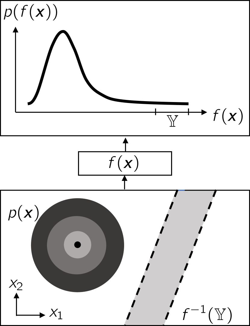
(a)

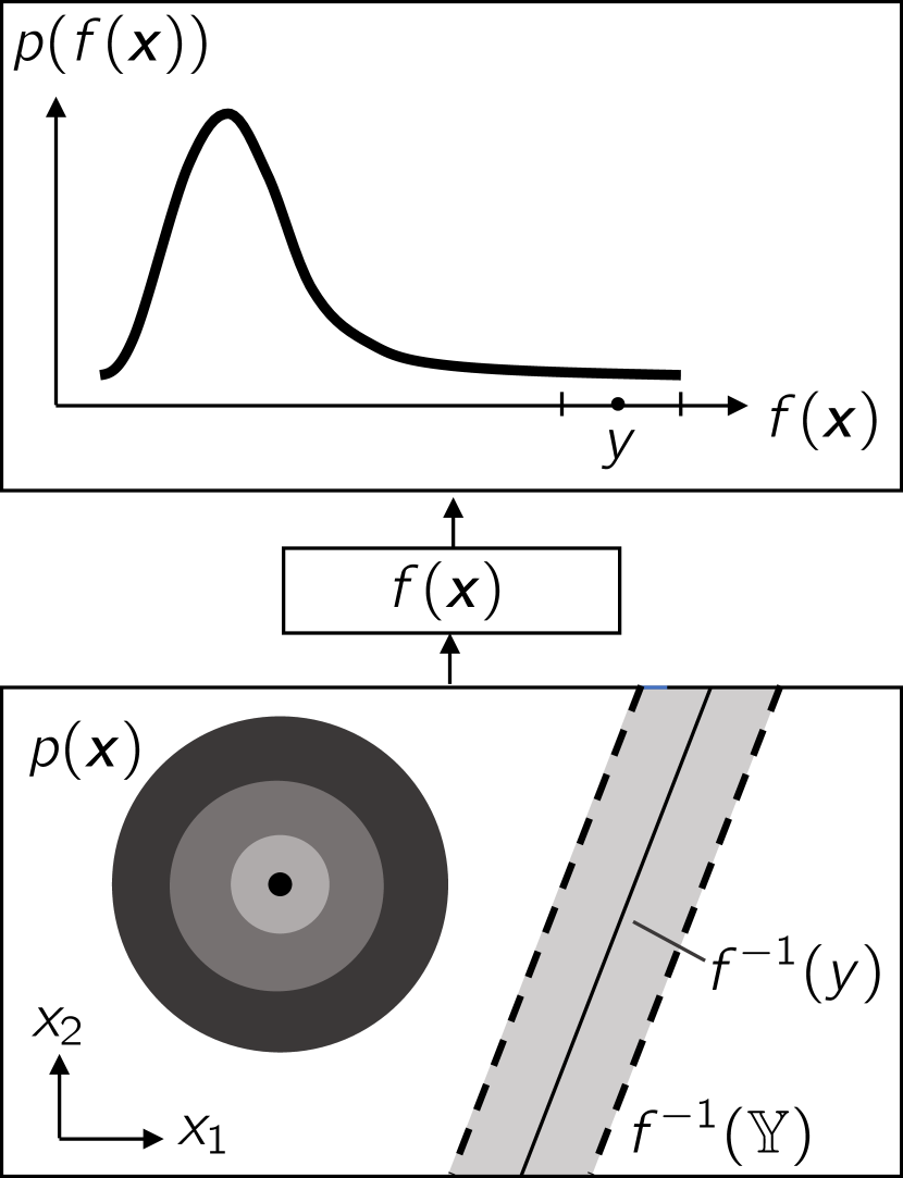
(b)

(c)

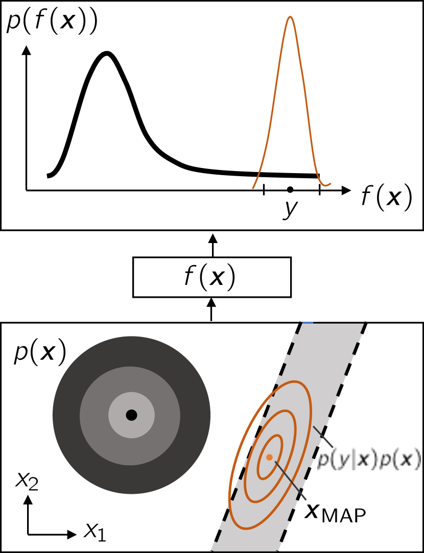
(d)

Figure 1: Summary of the BIMC methodology. In (1(a)), the problem statement is summarized - we need to compute the probability of the pre-image of the target interval, $f^{-1}(\mathbb{Y})$. In (1(b)), we introduce the pseudo-data point $y\in\mathbb{Y}$ and redefine $p(\bm{x})$ to be the pseudo-prior in a fictitious Bayesian inverse problem. The true inverse of the pseudo-data point $y$ is a straight line in $\mathbb{R}^{2}$. Next, in (1(c)), we select a pseudo-likelihood density, $p(y|\bm{x})$. The pseudo-likelihood density can also be viewed as a mollified approximation of the characteristic function. Part (1(d)) shows the contours of the posterior, $p(\bm{x}|y)$, which is proportional to $p(y|\bm{x})p(\bm{x})$. We use a Gaussian approximation to this posterior as an IS density.

Irrespective of the interpretation, this methodology introduces two tunable parameters—the pseudo-data $y\in\mathbb{Y}$ and variance of the pseudo-likelihood density, $\sigma^{2}$. These parameters can have a profound effect on the accuracy of the importance sampler and must be tuned with care. The tuning strategy depends on the nature of $f(\bm{x})$ as well as $p(\bm{x})$. Next, we discuss possible cases as well as the corresponding tuning strategy.

3.1 Affine $f$, Gaussian $p$

Although for a affine $f(\bm{x})$ and Gaussian $p(\bm{x})$, the probability $\mu=\mathbb{P}(f(\bm{x})\in\mathbb{Y})$ may be analytically computed, the availability of analytical expressions for $\bm{x}_{\mathrm{MAP}}$ and $\mathbf{H}_{\mathrm{GN}}$ in this case illustrates how our importance sampler achieves variance reduction. Let $f(\bm{x})=\bm{v}^{T}\bm{x}+\beta$, $p(\bm{x})=\mathcal{N}(\bm{x}_{0},\mathbf{\Sigma}_{0})$ for some $\bm{v}$, $\bm{x}_{0}\in\mathbb{R}^{m}$, $\beta\in\mathbb{R}$ and $\mathbf{\Sigma}_{0}\in\mathbb{R}^{m\times m}$. Then, $\mu$ is given analytically as

(9) $$\mu=\Phi\left(\frac{y_{\max}-\nu}{\gamma}\right)-\Phi\left(\frac{y_{\min}-\nu}{\gamma}\right),$$

where $\nu=\bm{v}^{T}\bm{x}_{0}+\beta$, $\gamma^{2}=\bm{v}^{T}\mathbf{\Sigma}_{0}\bm{v}$, and $\Phi$ is the standard Normal CDF.

Now, suppose the pseudo-data is some $y\in\mathbb{Y}$ and the variance of the pseudo-likelihood is some $\sigma^{2}\in\mathbb{R}$. Then the pseudo-posterior $p(\bm{x}|y)$ is also a Gaussian and no approximations are necessary. Hence, the IS density is given by $q(\bm{x})=\mathcal{N}(\bm{x}_{\mathrm{MAP}},\mathbf{H}_{\mathrm{GN}}^{-1})$, where,

(10) $$\bm{x}_{\mathrm{MAP}}=\bm{x}_{0}+\frac{y-f(\bm{x}_{0})}{\sigma^{2}+\bm{v}^{T}\mathbf{\Sigma}_{0}\bm{v}}\mathbf{\Sigma}_{0}\bm{v},\quad\mathbf{H}_{\mathrm{GN}}^{-1}=\mathbf{\Sigma}_{0}-\frac{1}{\sigma^{2}+\bm{v}^{T}\mathbf{\Sigma}_{0}\bm{v}}\big{(}\mathbf{\Sigma}_{0}\bm{v}\big{)}{\big{(}\mathbf{\Sigma}_{0}\bm{v}\big{)}}^{T}.$$

The expressions for $\bm{x}_{\mathrm{MAP}}$ and $\mathbf{H}_{\mathrm{GN}}^{-1}$ expose how our importance sampler achieves variance reduction. The MAP point identifies the region in parameter space where $f(\bm{x})\approx y$. The spread of the importance sampler, as encapsulated in its covariance, is reduced over its nominal value $\bm{\Sigma}_{0}$ in a direction informed by $\bm{v}$, the gradient of $f(\bm{x})$. Note that the reduction in variance occurs in just one direction, $\bm{\Sigma}_{0}\bm{v}$; the variance of $p(\bm{x})$ is retained in all other directions. The parameter $\sigma^{2}$ controls how much $q(\bm{x})$ is updated over $p(\bm{x})$- a small value for $\sigma$ results in a larger shift from $\bm{x}_{0}$ and a larger reduction in its spread. These claims become more transparent by noticing that the pushforward of $q(\bm{x})$ under $f$ is another Gaussian distribution in $\mathbb{R}$ (the pushforward density represents how $f(\bm{x})$ will be distributed if $\bm{x}$ is distributed according to $q(\bm{x})$). The mean $\chi$ and variance $\xi^{2}$ of this pushforward density are-

(11) $$\chi=(1-\rho^{2})y+\rho^{2}f(\bm{x}_{0}),\,\xi^{2}=\rho^{2}\bm{v}^{T}\bm{\Sigma}_{0}\bm{v},\,\text{where,}\,\rho^{2}=\frac{\sigma^{2}}{\sigma^{2}+\bm{v}^{T}\bm{\Sigma}_{0}\bm{v}}<1.$$

A small $\sigma$ implies small $\rho$, which means $\chi$ is closer $y$ and $\xi^{2}$ is small.

Since our goal is importance sampling, we wish to select those values for the tunable parameters that deliver just the right amount of update over $p$. We do this by minimizing the Kullback-Leibler (KL) divergence between $q(\bm{x})$ and the ideal IS distribution $q^{*}(\bm{x})$. Although not a true metric, the KL divergence between two probability densities is a measure of the distance between them. It is defined as:

(12) $$D_{\mathrm{KL}}(p||q)=\int p(\bm{x})\log\frac{p(\bm{x})}{q(\bm{x})}\mathrm{d}\bm{x}.$$

Then, the optimal pseudo-data point and the optimal variance of the pseudo-likelihood density can be obtained as:

(13) $$\begin{pmatrix}\sigma^{*}\\ y^{*}\end{pmatrix} =\operatorname*{arg\,min}_{\sigma,y}D_{\mathrm{KL}}(q^{*}||q;\sigma,y).$$

Analytic expressions for $D_{\mathrm{KL}}$, $y^{*}$, and $\sigma^{*}$ are derived for the affine Gaussian case in the supplement in LABEL:section:supplementAffineGauss. Selecting the tunable parameters in this way, in fact, allows us to make the following claim regarding the resulting IS distribution:

Claim 1 (BIMC optimality).

In the affine-Gaussian case, the importance sampling density that results from the BIMC procedure is equivalent to the Gaussian distribution closest in KL divergence to $q^{*}(\bm{x})$.

Proof 3.1.

Proof given in the supplement in LABEL:section:supplementAffineGauss:

Hence, BIMC is implicitly searching for the best Gaussian approximation of $q^{*}(\bm{x})$. A Gaussian distribution in $m$ dimensions has ${m(m+1)}/{2}$ free variables, so a naive search for the best Gaussian approximation of $q^{*}(\bm{x})$ will optimize over all $\mathcal{O}(m^{2})$ free variables. However, BIMC accomplishes this task be optimizing just 2 free variables. This can be attributed to the similar structure of the pseudo-posterior ${p(y|\bm{x})p(\bm{x})}/{p(y)}$, and the ideal IS density, ${\bm{\mathrm{1}}_{\mathbb{Y}}(f(\bm{x}))p(\bm{x})}/{\mu}$.

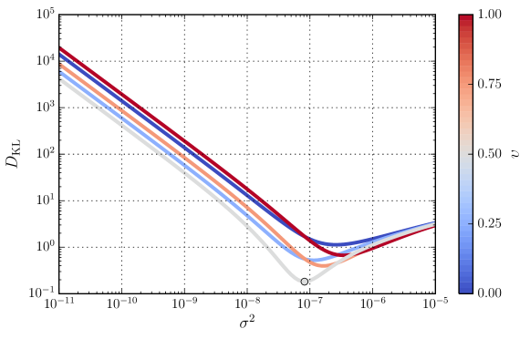
Figure 2: This figure shows the variation of $D_{\mathrm{KL}}$ at various values of the data point $y$ and pseudo-likelihood variance $\sigma^{2}$. Here, the data point $y$ has been normalized to $\upsilon=(y-y_{\min})/(y_{\max}-y_{\min})$ and $f(\bm{x})$ is an affine transformation from $\mathbb{R}^{100}$ to $\mathbb{R}$. The marker shows the $(\sigma,\upsilon)$ combination that resulted from numerical minimization of $D_{\mathrm{KL}}$.

To verify whether minimizing $D_{\mathrm{KL}}$ to obtain parameters actually translates to improved performance of our IS density, we synthesized a affine map from $\mathbb{R}^{100}$ to $\mathbb{R}$ (implementation details are provided in the supplement in LABEL:supplement:fwdModels). We measure performance by the relative RMSE in the probability estimate, $\tilde{e}_{\mathrm{RMS}}$, and we expect $\tilde{e}_{\mathrm{RMS}}$ to be small when $y=y^{*}$ and $\sigma=\sigma^{*}$. In addition, in this case, $\mu$ is available to us analytically. This provides yet another indicator of performance- the absolute difference between the analytical value and the IS estimate must be small when the optimal parameters are being used.

Figure 2 shows the variation of $D_{\mathrm{KL}}$ with $\sigma^{2}$ at various $y$ in addition to the optimal $(\sigma,y)$ combination that results from numerical optimization. We conclude the following from the figure:

• The optimal pseudo-data point lies almost exactly at the mid-point of $\mathbb{Y}$.

• $D_{\mathrm{KL}}$ is extremely sensitive to the spread of the pseudo-likelihood probability density $\sigma$, much more so than the pseudo-data $y$. Intuitively, a large value for $\sigma$ emphasizes the pseudo-prior over the data so that sampling from $q(\bm{x})$ is akin to sampling from $p(\bm{x})$. On the other hand, too small a value for $\sigma^{2}$ results in $q(\bm{x})$ not having enough spread to cover the region where $f(\bm{x})\in\mathbb{Y}$, which could result in significant bias when the number of samples is small.

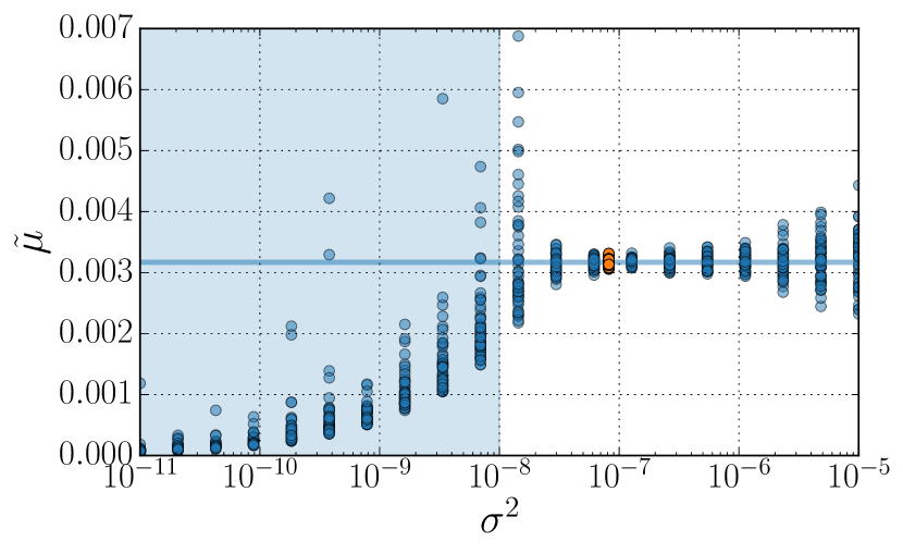
(a) The IS probability estimate $\tilde{\mu}$ against $\sigma^{2}$ at $y=y^{*}$. Each marker indicates $\tilde{\mu}$ from an individual run. The solid line indicates the true value of $\mu$. The markers in orange denote runs at $\sigma=\sigma^{*}$.

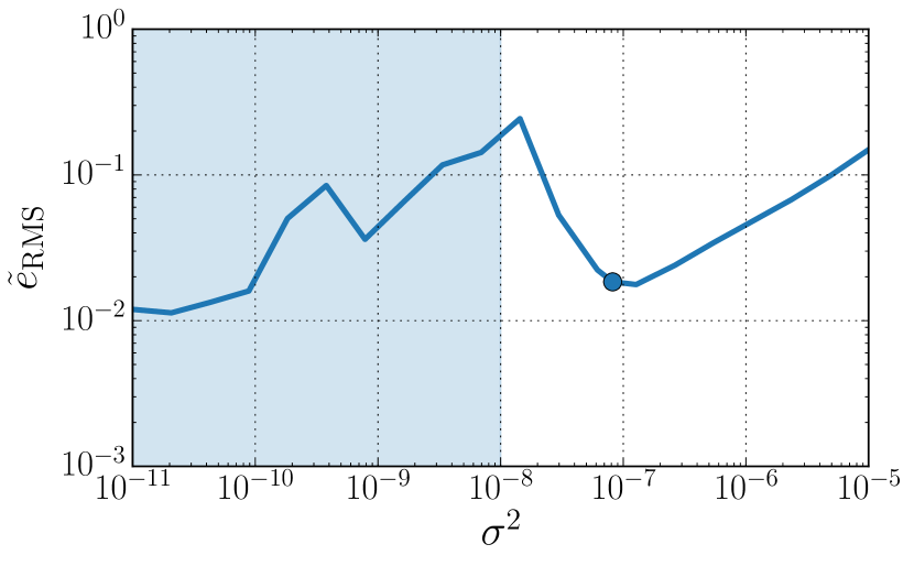
(b) The relative RMSE $\tilde{e}_{\mathrm{RMS}}$ against $\sigma^{2}$ at $y=y^{*}$. Only the average $\tilde{e}_{\mathrm{RMS}}$ over all runs at fixed $\sigma^{2}$ is plotted. The marker is at $\sigma=\sigma^{*}$.

Figure 3: This figure shows the variation of the probability estimate $\tilde{\mu}$ and the relative RMSE $\tilde{e}_{\mathrm{RMS}}$ with the likelihood variance $\sigma^{2}$. At fixed $\sigma^{2}$, we performed 50 independent runs using $N=1000$ samples. For $\tilde{\mu}$, we plot the probability estimate obtained from each run, whereas for $\tilde{e}_{\mathrm{RMS}}$, we plot the ensemble average at each $\sigma$.

In Figure 3, we fix $y=y^{*}$ and plot the variation of the probability estimate, $\tilde{\mu}$, and the relative RMSE, $\tilde{e}_{\mathrm{RMS}}$, with $\sigma^{2}$. For each value of $\sigma^{2}$, we performed several independent runs. Figure 3(a) plots $\tilde{\mu}$ obtained from each run. In Figure 3(b), we plot the ensemble average of $\tilde{e}_{\mathrm{RMS}}$ over all simulations at fixed $\sigma^{2}$. Both figures demonstrate that when $\sigma^{2}$ is small, both the probability estimate and the associated RMSE have significant bias (shaded region in the figures). When $\sigma^{2}$ is large, error increases with $\sigma^{2}$ since the emphasis on pseudo-data decreases. There lies an optimal $\sigma^{2}$ somewhere in between, and indeed, minimizing $D_{\mathrm{KL}}$ helps identify it. So far we’ve been using just one pseudo-data point $y\in\mathbb{Y}$. However, it is also possible to use multiple pseudo-data points, $\{y_{i}\}_{i=1}^{n},y_{i}\in\mathbb{Y}$. In this case, using the same pseudo-likelihood density for all $y_{i}$, a posterior $p(\bm{x}|y_{i})$ and its corresponding Gaussian approximation can be obtained for each $y_{i}$. These Gaussians can then be collected into a mixture distribution to form the IS density. So, a possibility is to use the following IS density:

(14) $$q(\bm{x})=\frac{1}{n}\sum_{i=1}^{n}\mathcal{N}\left(\bm{x}_{\mathrm{MAP}}^{(i)},{\left(\mathbf{H}^{(i)}_{\mathrm{GN}}\right)}^{-1}\right).$$

where $\bm{x}_{\mathrm{MAP}}^{(i)}$ is the MAP point corresponding to $y_{i}$ and $\mathbf{H}_{\mathrm{GN}}^{(i)}$ is the Hessian matrix of $-\log p(\bm{x}|y_{i})$ at $\bm{x}_{\mathrm{MAP}}^{(i)}$. Next, we investigate whether using $n>1$ pseudo-data points in $\mathbb{Y}$ leads to better performance than using just one pseudo-data point, i.e., $n=1$.

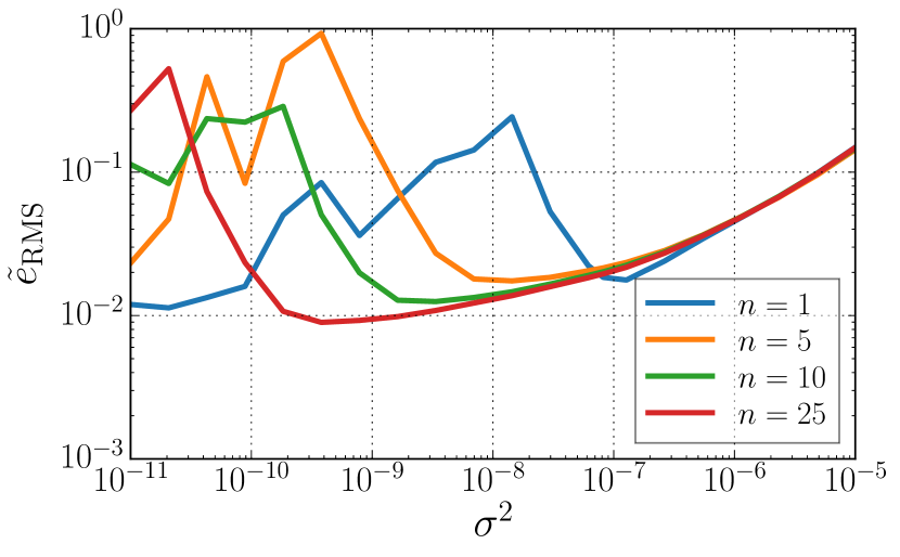
(a) Linear inverse problem.

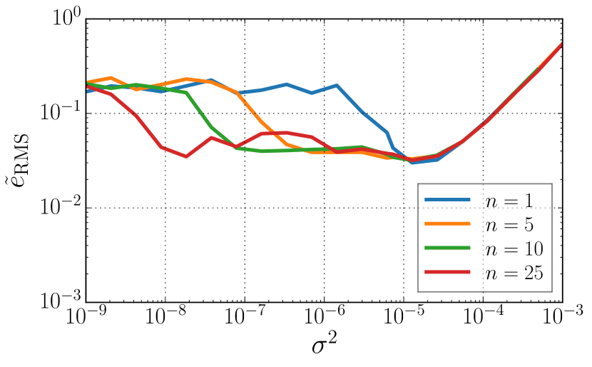
(b) Synthetic non-linear problem.

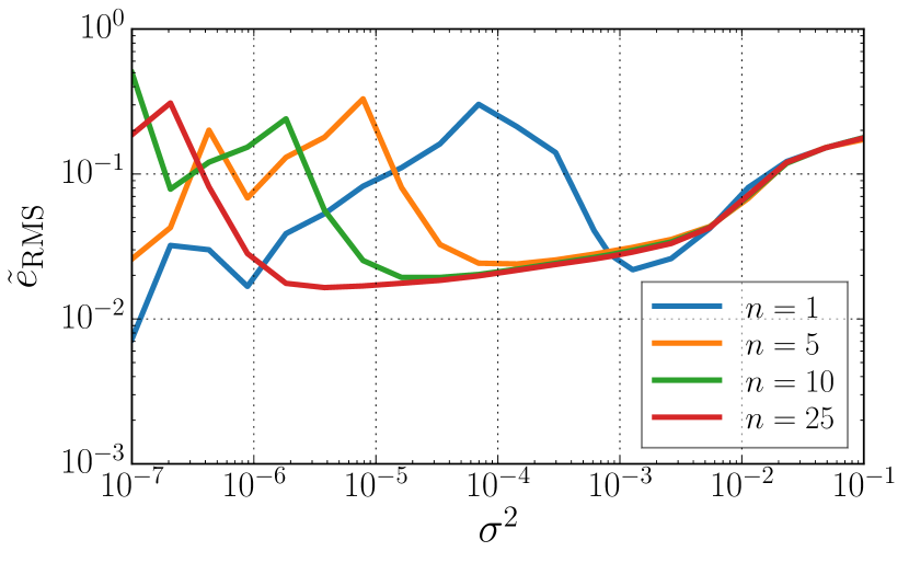
(c) Single step reaction.

(d) Elliptic PDE.

Figure 4: This figure shows how $\tilde{e}_{\mathrm{RMS}}$ varies with $\sigma^{2}$ at different values of $n$ for various forward models. At fixed $\sigma^{2}$, we perform 50 independent simulations and report the ensemble averaged $\tilde{e}_{\mathrm{RMS}}$. When $n=1$, we use the optimal data point obtained employing the appropriate tuning strategy described in the text. When $n>1$, we select $n$ evenly spaced points in $\mathbb{Y}$. Similar to Figure 3, IS estimates are biased when $\sigma^{2}$ is small. The extent of the biased regions depends on $n$ and appears to decrease as $n$ increases.

To ensure a fair comparison between the two cases, they must each be run using their respective optimal parameters. When $n>1$, the tunable parameters are the number of pseudo-data points, $n$, their values, $\{y_{i}\}_{i=1}^{n}$, and the variance of the common pseudo-likelihood density, $\sigma^{2}$. However, minimizing the Kullback-Leibler distance between $q$ and $q^{*}$ to obtain parameters is no longer possible. This is because the Kullback-Leibler distance between two Gaussian mixtures doesn’t have a closed form expression [11]. To proceed, given $n>1$, we fix $\{y_{i}\}$ to be $n$ evenly spaced points in $\mathbb{Y}$. We then sweep over several values of $n$ and $\sigma^{2}$ to investigate whether increasing $n$ has any advantages.

Empirical evidence seems to suggest no. In Figure 4, we plot the variation of the ensemble averaged $\tilde{e}_{\mathrm{RMS}}$ with $\sigma^{2}$ at various values of $n$ and using various forward models, both linear and non-linear (details of the forward models are provided in the supplement in LABEL:supplement:fwdModels). While the error decreases with increasing $n$ for some cases, we believe the decrease isn’t large enough to justify the increased computational cost of solving additional inverse problems.

Figure 5: Arbitrary unimodal $p$. In this case, the true posterior and the ideal IS density are multimodal. The optimizer used for computing $\bm{x}_{\mathrm{MAP}}$ will only find one of these modes. Our IS density will then only sample around that mode, leading to incorrect estimates.

3.2 Affine $f$, mixture-of-Gaussians $p$

If $p(\bm{x})$ is a mixture of Gaussians, $p(\bm{x})=\sum_{i=1}^{k}w_{i}p_{i}(\bm{x})$, then, notice that,

(15) $$\mu=\int\bm{\mathrm{1}}_{\mathbb{Y}}\left(f(\bm{x})\right)p(\bm{x})\mathrm{d}\bm{x}=\sum_{i=1}^{k}w_{i}\int\bm{\mathrm{1}}_{\mathbb{Y}}\left(f(\bm{x})\right)p_{i}(\bm{x})\mathrm{d}\bm{x}=\sum_{i=1}^{k}w_{i}\mu_{i}$$

The contribution to $\mu$ from each component $p_{i}(\bm{x})$, $\mu_{i}$, can then be calculated using BIMC as described above. If $\tilde{\mu}_{i}$ is the estimate from each component, $\mu$ can be estimated as $\tilde{\mu}=\sum_{i=1}^{k}w_{i}\tilde{\mu}_{i}$.

3.3 Affine $f$, arbitrary unimodal $p$

In this case, even though $p$ is unimodal, $q^{*}$, and the pseudo-posterior $p(\bm{x}|y)$, can be multi-modal (see Figure 5). Then, depending on the initial guess provided, the optimizer used for computing the MAPs may converge to only one of the modes. A local Gaussian characterization of the pseudo-posterior will only sample near this mode and all the other modes will be ignored. This will cause $\mu$ to be underestimated. To avoid this, we propose approximating $p$ with a mixture of Gaussians and then proceeding with the methodology outlined in the previous section. This will lead to an estimate whose accuracy is as good as the accuracy in approximating $p$ with a mixture of Gaussians.

3.4 Non-linear $f$, Gaussian $p$

When $f(\bm{x})$ is non-linear, the KL divergence may not have a tractable closed-form expression even when only one pseudo-data point is used. Although a sample based estimate of the KL divergence can be obtained, it would require evaluating $f(\bm{x})$ for each sample, increasing the cost of constructing the IS density. To compute the optimal parameters in this case, we instead propose linearizing $f(\bm{x})$ around the MAP point corresponding to an initial pseudo-data point, $y^{\mathrm{mid}}=\mathrm{mid}\,\mathbb{Y}$, which we denote $\bm{x}_{\mathrm{MAP}}^{\mathrm{mid}}$. This necessitates solving another optimization problem (as in Equation 7), for which we require $\sigma^{2}$, a quantity we set out to tune in the first place. However, this $\sigma^{2}$ is only used to construct the linearization and has little bearing on subsequent sampling. We recommend setting $\sigma=0.1(y_{\max}-y_{\min})$. Once we have $\bm{x}_{\mathrm{MAP}}^{\mathrm{mid}}$, we linearize $f(\bm{x})$ as follows:

(16) $$f(\bm{x})\approx f(\bm{x}_{\mathrm{MAP}}^{\mathrm{mid}})+\mathbf{J}^{\mathrm{mid}}(\bm{x}-\bm{x}_{\mathrm{MAP}}^{\mathrm{mid}})$$

Here, $\mathbf{J}^{\mathrm{mid}}\in\mathbb{R}^{1\times m}$ is the Jacobian matrix of the $f(\bm{x})$ evaluated at $\bm{x}_{\mathrm{MAP}}^{\mathrm{mid}}$. From here on, we can proceed to obtain the optimal parameters as in the affine case by identifying $\bm{v}^{T}\equiv\mathbf{J}^{\mathrm{mid}}$ and $\beta\equiv f(\bm{x}_{\mathrm{MAP}}^{\mathrm{mid}})-\mathbf{J}^{\mathrm{mid}}\bm{x}_{\mathrm{MAP}}^{\mathrm{mid}}$. Note that such a procedure will not reveal the true optimal parameters that correspond to the non-linear forward model. It only provides an estimate, but allows us to use analytically derived expressions and keep computational costs low. Another consequence of linearizing $f(\bm{x})$ is that it allows for the analytical computation of the rare event probability associated with the linearized map (Equation 9). We will refer to this estimate of $\mu$ as the linearized probability estimate, $\mu_{\mathrm{lin}}$.

3.5 Non-linear $f$, mixture-of-Gaussian $p$

This case is similar to Section 3.2. Recall that $\mu$ is just the weighted sum of probability corresponding to each component mixtures, $\mu_{i}$. Each $\mu_{i}$ can be estimated by the method outlined above, and then weighed and summed to obtain an estimate for $\mu$.

Procedure 1 BIMC

1:$f(\bm{x})$, $p(\bm{x})$, $\mathbb{Y}$, $N$

2:$\tilde{\mu}$

3:% Select optimal parameters, $y^{*},\sigma^{*}$

4:$y^{\max}\leftarrow\max\mathbb{Y}$, $y^{\min}\leftarrow\min\mathbb{Y}$, $y^{\mathrm{mid}}\leftarrow 0.5(y^{\mathrm{min}}+y^{\mathrm{max}})$

5:$\sigma_{0}\leftarrow 0.1(y^{\max}-y^{\min})$

6:$\bm{x}_{\mathrm{MAP}}^{\mathrm{mid}}\leftarrow\texttt{getMAP}(y_{\mathrm{mid}},\sigma_{0})$ % Minimize Equation 6 using $y=y^{\mathrm{mid}},\sigma=\sigma_{0}$

7:$\bm{v}^{T}\leftarrow\left.\frac{\partial f(\bm{x})}{\partial\bm{x}}\right|_{\bm{x}=\bm{x}_{\mathrm{MAP}}}$

8:$\beta\leftarrow f(\bm{x}_{\mathrm{MAP}}^{\mathrm{mid}})-\bm{v}^{T}\bm{x}_{\mathrm{MAP}}^{\mathrm{mid}}$

9:$(y^{*},\sigma^{*})\leftarrow\texttt{minimizeKLDiv}(\bm{v},\beta,p)$ % Minimize $D_{\mathrm{KL}}(q^{*}||q)$ as in LABEL:dkl

10:

11:% Build IS density using optimal parameters

12:$\bm{x}_{\mathrm{MAP}}\leftarrow\texttt{getMAP}(y^{*},\sigma^{*})$ % Minimize Equation 6 using $y=y^{*},\sigma=\sigma^{*}$

13:$\mathbf{H}_{\mathrm{GN}}\leftarrow\texttt{getHessian}(\bm{x}_{\mathrm{MAP}},y^{*},\sigma^{*})$ % Compute Hessian of Equation 6 at $\bm{x}_{\mathrm{MAP}}$ using $y=y^{*},\sigma=\sigma^{*}$

14:$q(\bm{x})\leftarrow\mathcal{N}(\bm{x}_{\mathrm{MAP}},\mathbf{H}_{\mathrm{GN}}^{-1})$

15:

16:% Sample from $q$ to estimate $\mu$

17:for $i=1,\ldots,N$ do

18:     $\bm{x}_{i}\sim q(\bm{x})$

19:     $w_{i}\leftarrow\bm{\mathrm{1}}_{\mathbb{Y}}(f(\bm{x}_{i}))p(\bm{x}_{i})/q(\bm{x}_{i})$

20:end for

21:$\tilde{\mu}\leftarrow\sum_{i=1}^{N}w_{i}/N$

22:return $\tilde{\mu}$

3.6 Summary

To summarize, in this section we described how a fictitious Bayesian inverse problem can be constructed from the components of the forward UQ problem. The solution of this fictitious inverse problem yields a posterior whose Gaussian approximation is our IS density. The parameters on which the IS density depends can be tuned by minimizing an analytical expression for its Kullback-Leibler divergence with respect to the ideal IS density. A drawback of our method is that we’re restricted to nominal densities that are Gaussian mixtures or easily approximated by one. The overall algorithm for arbitrary, non-linear $f$ is given in Algorithm 1. Next, we present and discuss results of our numerical experiments.

4 Experiments

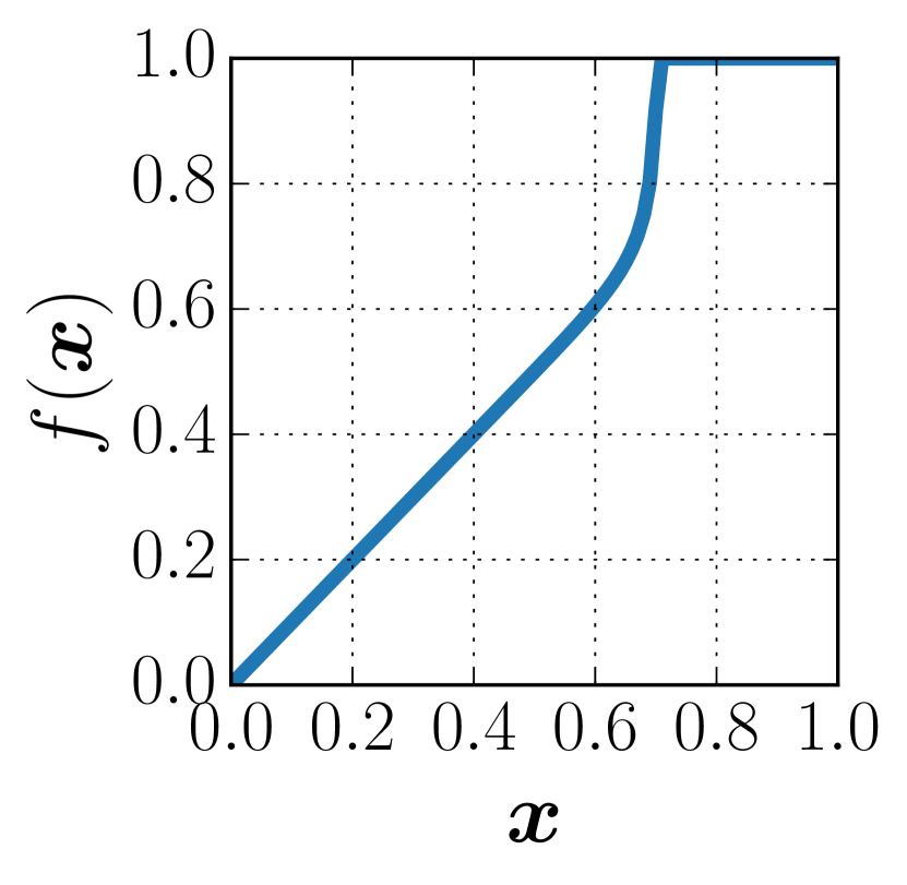
(a) Single step reaction

(b) Autoignition

(c) Synthetic non-linear

Figure 6: Non-linearity of $f$. For the single step reaction problem, we plot the full forward map $f$ for all possible values of the input $\bm{x}$. For the autoignition and synthetic non-linear problems, we demonstrate how $\nabla f(\bm{x})$ varies. We draw samples, $\bm{x}_{i}$, from $p(\bm{x})$, and evaluate $\|\nabla f(\bm{x})-\nabla f(\bm{x}_{0})\|/\|\nabla f(\bm{x}_{0})\|$, where $\bm{x}_{0}$ is the prior mean. Departure from 0 of this quantity signifies the degree of non-linearity.

In this section, we present results that demonstrate the efficacy of our method. We also report cases where our method fails (detailed discussion about failure mechanisms of BIMC is postponed to the end of this section). The forward models we used in our experiments are briefly summarized below. A detailed description of the models and the problem setup is given in the supplement in LABEL:supplement:fwdModels. Figure 6 shows the variation of $f$ for select models and demonstrates that it is indeed non-linear.

• Affine case: In this case $f(\bm{x})$ is a affine map from $\mathbb{R}^{m}$ to $\mathbb{R}$. We choose $m=2$ for illustration, and $m=100$ for comparison with MC.

• Synthetic non-linear problem: In this case, $f(\bm{x})$ is defined to be the following map from $\mathbb{R}^{m}$ to $\mathbb{R}$.

  (17) $$f(\bm{x})=\bm{o}^{T}\bm{u},\,\text{where}\left(\mathbf{S}+\varepsilon\bm{x}\bm{x}^{T}\right)\bm{u}=\bm{b}.$$

  Here, $\varepsilon\in\mathbb{R}$, $\bm{o},\bm{u},\bm{b}\in\mathbb{R}^{m}$, and $\mathbf{S}\in\mathbb{R}^{m\times m}$. Again, $m=2$ was chosen for illustration and $m=10$ for comparison with MC.

• Single step reaction: The forward model here describes a single step chemical reaction using an Arrhenius type rate equation. A progress variable $u\in\left[0,1\right]$ is used to describe the reaction. The parameter $\bm{x}$ is the initial value of progress variable $u(0)$ and the observable $f(\bm{x})$ is the value of the progress variable at some final time $t_{f},u(t_{f})$. Thus $f(\bm{x})$ is a map from $\mathbb{R}$ to $\mathbb{R}$.

• Autoignition: Here, we allow a mixture of hydrogen and air to undergo autoignition in a constant pressure reactor. A simplified mechanism with 5 elementary involving 8 chemical species is used to describe the chemistry. The parameter $\bm{x}$ is the vector of the initial equivalence ratio, initial temperature and the initial pressure in the reactor and the observable is the amount of heat released so that $f(\bm{x})$ is a map from from $\mathbb{R}^{3}$ to $\mathbb{R}$.

• Elliptic PDE: In this system, we invert for the discretized log-permeability field in some spatial domain given an observation of the pressure at some point. The forward problem, that is, obtaining the pressure from the log-permeability field, is governed by an elliptic PDE. A finite element discretization results in $f(\bm{x})$ being a map from $\mathbb{R}^{4225}$ to $\mathbb{R}$.

• The Lorenz system: Here, the forward problem is governed by the chaotic Lorenz equations [18]. The parameter $\bm{x}$ is the initial condition of the system while the observable is value of the first component of the state vector at some final time $t_{f}$. We simulate the Lorenz system over three time horizons, $t_{f}=0.1$s, $t_{f}=5$s, and $t_{f}=15$s. BIMC fails over longer time horizons, i.e., when $t_{f}=5$s and $t_{f}=15$s.

• Periodic case: Here, $f(\bm{x})$ is a periodic function in $\mathbb{R}^{2}$, $f(\bm{x})=\sin(x_{1})\cos(x_{2})$. This is another case when BIMC fails.

Sampling illustration

We begin by presenting examples in low-dimensions that illustrate the quality of samples from BIMC. In Figure 7, we compare samples generated using MC and BIMC. We also depict the ideal IS density $q^{*}$ in the figures, either using contours, or through samples. As expected, the variance of the IS density in our method is only decreased in one data-informed direction. The extent of this decrease depends on the variance of the pseudo-likelihood density, $p(y|\bm{x})$, and a tuning algorithm based on minimizing the Kullback-Leibler distance leads to a good fit between the spread of $q^{*}(\bm{x})$ and $q(\bm{x})$ in this direction. In all other directions, the spread of $q(\bm{x})$ is same as that of $p(\bm{x})$. This is because the pseudo-data $y$ does not inform these directions.

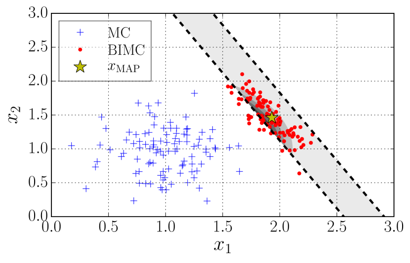
(a) The affine case.

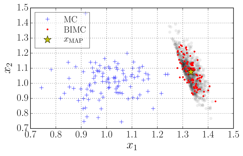
(b) The synthetic non-linear case.

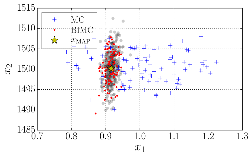
(c) Autoignition, $x_{1}$ - $x_{2}$ plane.

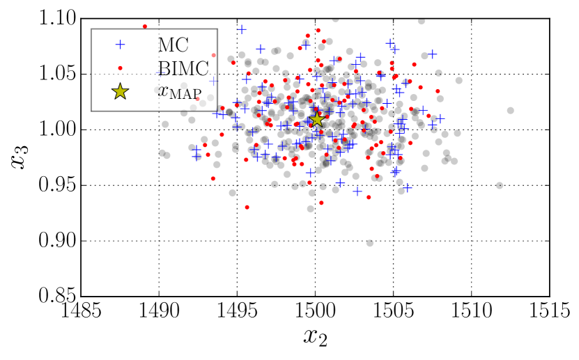
(d) Autoignition, $x_{2}$ - $x_{3}$ plane.

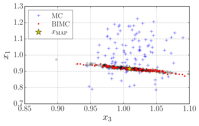
(e) Autoignition, $x_{3}$ - $x_{1}$ plane.

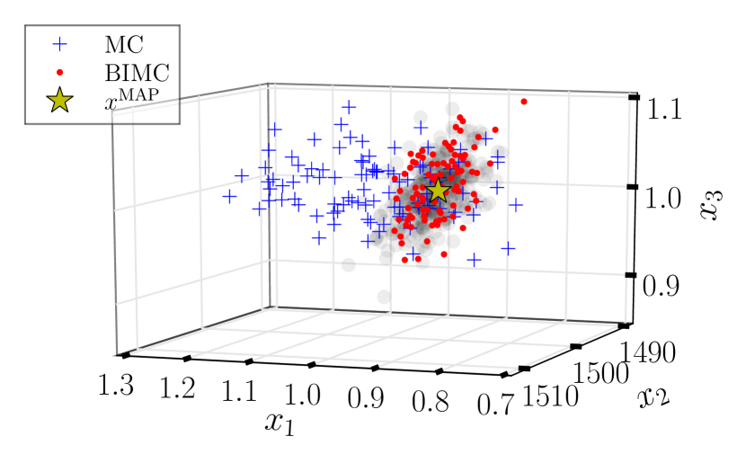
(f) Autoignition, 3D view.

Figure 7: Sampling illustration. In this figure, we plot 100 samples from $p(\bm{x})$ (which corresponds to vanilla MC) as well as $q(\bm{x})$ (which corresponds to BIMC) with $n=1$ for the affine, synthetic non-linear, and the autoignition problems. For the affine case (7(a)), the region in $\mathbb{R}^{2}$ that evaluates inside $\mathbb{Y}$ is analytically available and is plotted between the thick, dashed lines. Also analytically available is the ideal IS density $q^{*}$ whose contours are plotted. For all other forward models, a scatter plot of samples drawn from $q^{*}$ is used to represent its magnitude.

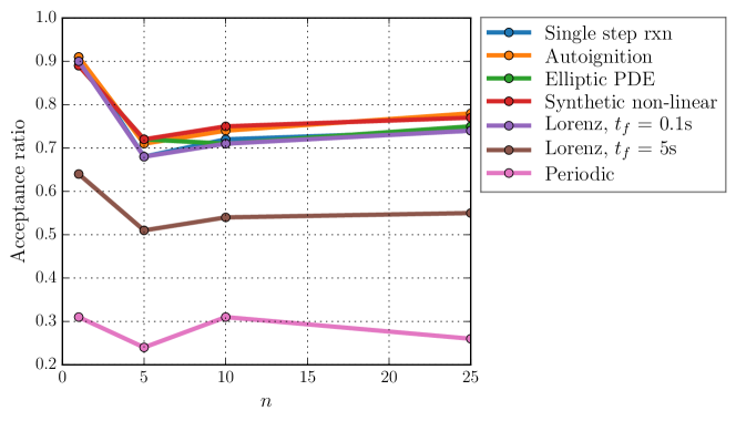
Figure 8: Fraction of samples that evaluate inside $\mathbb{Y}$ for the different forward models at various values of $n$. In this experiment $N=1000$ and $\mu$ spans two orders of magnitude, from $\mathcal{O}(10^{-2})$ to $\mathcal{O}(10^{-4})$. The BIMC methodology fails for the periodic and Lorenz, $t_{f}=5$s cases, hence the lower acceptance ratio.

As a quantitative estimate of the quality of samples, we report the acceptance ratio, defined as the fraction of samples that evaluate inside $\mathbb{Y}$. The acceptance ratio resulting from BIMC is plotted in Figure 8 (the acceptance ratio from MC on the other hand is $\hat{\mu}$ by definition). We observe that $n=1$ consistently leads to an acceptance ratio of around 90% irrespective of $\mu$ (except in the Periodic and Lorenz, $t_{f}=5$s cases; these are failure cases and will be discussed at the end of this section). The slight dip in the acceptance ratio when $n>1$ can be attributed to the effect of always having $y_{\min}$ and $y_{\max}$ as data points. Because these points lie at the edge of the interval $\mathbb{Y}$, they lead to an increased number of samples that are close to these limit points, but don’t actually evaluate inside $\mathbb{Y}$. As $n$ increases however, the number of samples drawn from mixture components corresponding to these two points decreases and the acceptance ratio shows an upward trend.

Convergence with number of samples

Next, we compare the relative RMS error, $e_{\mathrm{RMS}}$, from MC and BIMC in Figure 9. BIMC offers the same accuracy using far fewer number of samples and results in an order of magnitude or more of speedup. The exact speedup achieved depends on the magnitude of the probability. In addition, there is little asymptotic effect of using $n>1$. The corresponding probability estimates are presented in the supplement in LABEL:supplement:results.

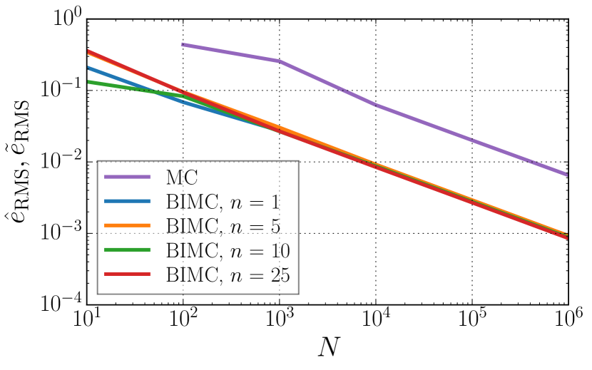
(a) Single step reaction, $\mu\approx 2.30\times 10^{-2}$.

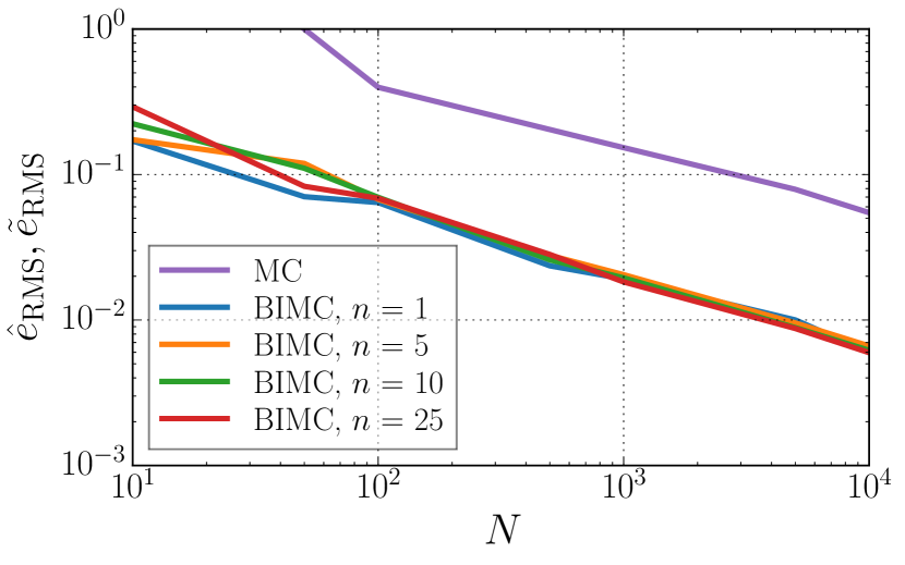
(b) Autoignition, $\mu\approx 3.24\times 10^{-2}$.

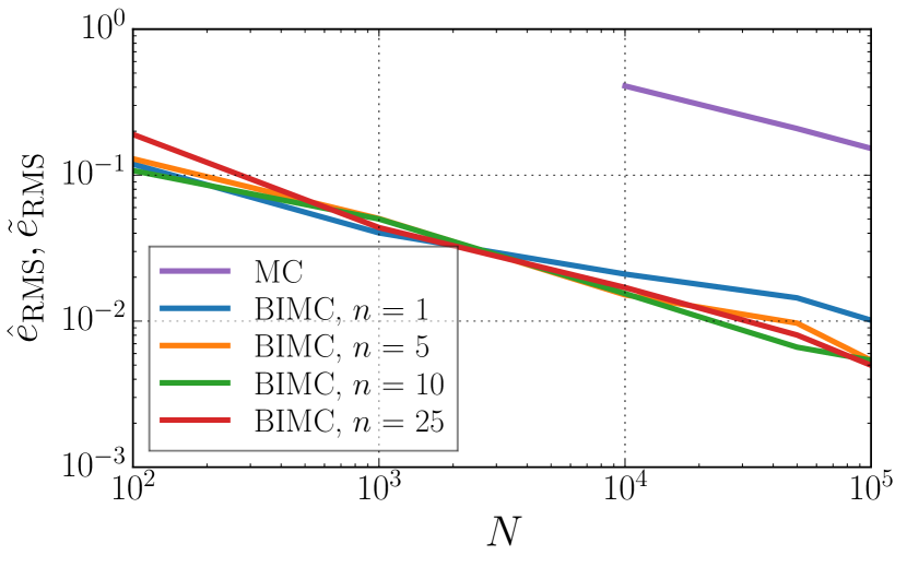
(c) Elliptic PDE, $\mu\approx 3.91\times 10^{-4}$.

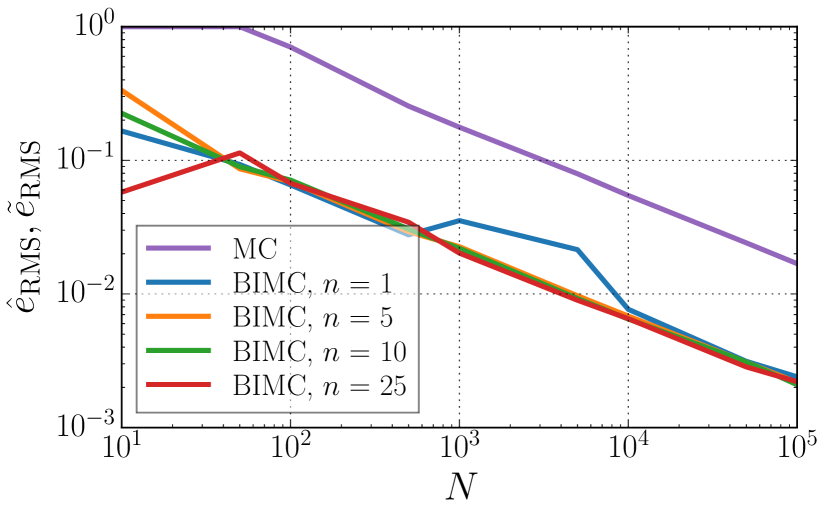
(d) Lorenz, $t_{f}$ = 0.1s., $\mu\approx 3.28\times 10^{-2}$.

Figure 9: Comparison of performance of MC and BIMC. The variation of the relative RMSE, $e_{\mathrm{RMS}}$, is plotted against the number of samples $N$. For reference, the most accurate probability estimate is also reported.

Effect of probability magnitude

In Figure 10, we study the effect of the probability magnitude on the relative RMSE, $\tilde{e}_{\mathrm{RMS}}$. We notice that BIMC is only weakly dependent on the probability magnitude. This is because selecting parameters by minimizing $D_{\mathrm{KL}}$ leads to an IS density that is optimally adapted for sampling around $\mathbb{Y}$.

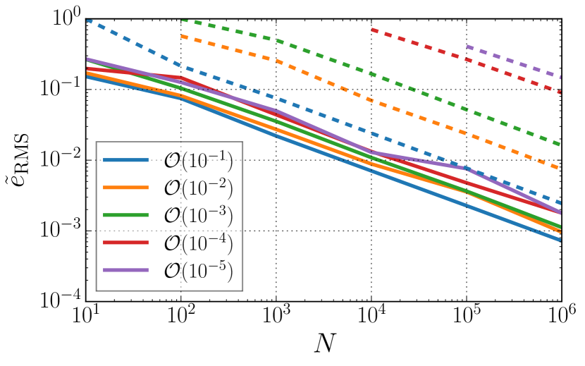
(a) Synthetic non-linear problem

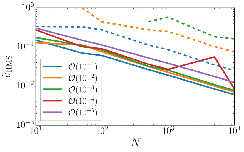
(b) Autoignition

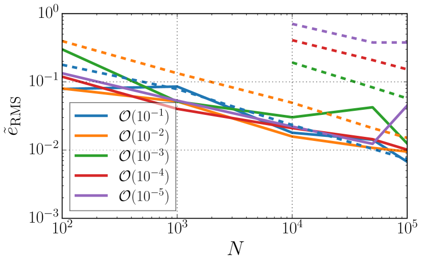
(c) Elliptic PDE

Figure 10: Effect of varying probability levels. In this figure, we plot the variation of ensemble averaged relative $\tilde{e}_{\mathrm{RMS}}$ with the number of samples $N$ for various forward models with varying levels of probability. The varying probability levels are selected by moving $\mathbb{Y}$ to the tail regions of $p(\bm{x})$. The dashed lines indicate errors associated with MC while the solid lines indicate errors in BIMC.

Extremely rare events

In our final experiment, we push BIMC to compute probabilities of extremely rare events. The rare events were constructed by shifting $\mathbb{Y}$ further and further into the tail region of the push forward of $p(\bm{x})$ under $f$. BIMC is able to compute extremely small probabilities using a modest number of samples. This experiment also corroborates our claim that the accuracy of our method is only weakly dependent on the probability magnitude $\mu$. We also report the probability estimate resulting from linearizing $f(\bm{x})$ around $\bm{x}^{\mathrm{mid}}$ and conclude that the linearized probability estimate is a good indicator of the order of magnitude of the true probability.

Table 2: Extremely rare events, $N$ = 1000.

BIMC, $n=1$		BIMC, $n=5$		Linearized
$\tilde{\mu}^{N}$	$\tilde{e}_{\mathrm{RMS}}^{N}$	$\tilde{\mu}^{N}$	$\tilde{e}_{\mathrm{RMS}}^{N}$	$\mu_{\mathrm{lin}}$
$3.6214\times 10^{-3}$	$3.24\times 10^{-2}$	$3.7892\times 10^{-3}$	$3.87\times 10^{-2}$	$5.9770\times 10^{-3}$
$2.3938\times 10^{-6}$	$6.00\times 10^{-2}$	$2.1421\times 10^{-6}$	$6.10\times 10^{-2}$	$1.8252\times 10^{-6}$
$5.4224\times 10^{-8}$	$6.64\times 10^{-2}$	$5.4310\times 10^{-8}$	$7.08\times 10^{-2}$	$4.2072\times 10^{-8}$
$5.7578\times 10^{-10}$	$1.04\times 10^{-1}$	$5.6271\times 10^{-10}$	$6.79\times 10^{-2}$	$3.8026\times 10^{-10}$

(a) Synthetic non-linear problem

$n=1$		$n=5$		Linearized
$\tilde{\mu}^{N}$	$\tilde{e}_{\mathrm{RMS}}^{N}$	$\tilde{\mu}^{N}$	$\tilde{e}_{\mathrm{RMS}}^{N}$	$\mu_{\mathrm{lin}}$
$4.3626\times 10^{-3}$	$2.47\times 10^{-2}$	$4.3688\times 10^{-3}$	$3.52\times 10^{-2}$	$4.5667\times 10^{-3}$
$1.1158\times 10^{-5}$	$3.91\times 10^{-2}$	$1.1278\times 10^{-5}$	$4.52\times 10^{-2}$	$8.4646\times 10^{-5}$
$7.6348\times 10^{-7}$	$5.86\times 10^{-2}$	$8.0428\times 10^{-7}$	$7.76\times 10^{-2}$	$3.8022\times 10^{-6}$
$3.5977\times 10^{-10}$	$9.69\times 10^{-2}$	$3.8106\times 10^{-10}$	$1.54\times 10^{-1}$	$2.6634\times 10^{-10}$

(b) Autoignition

$n=1$		$n=5$		Linearized
$\tilde{\mu}^{N}$	$\tilde{e}_{\mathrm{RMS}}^{N}$	$\tilde{\mu}^{N}$	$\tilde{e}_{\mathrm{RMS}}^{N}$	$\mu_{\mathrm{lin}}$
$2.6422\times 10^{-3}$	$5.05\times 10^{-2}$	$2.7045\times 10^{-3}$	$3.90\times 10^{-2}$	$2.2526\times 10^{-3}$
$5.6726\times 10^{-6}$	$9.44\times 10^{-2}$	$5.1764\times 10^{-6}$	$4.76\times 10^{-2}$	$4.1409\times 10^{-6}$
$8.4630\times 10^{-9}$	$4.94\times 10^{-2}$	$8.6889\times 10^{-9}$	$5.58\times 10^{-2}$	$8.7048\times 10^{-9}$
$8.2730\times 10^{-10}$	$4.99\times 10^{-2}$	$8.0669\times 10^{-10}$	$7.36\times 10^{-2}$	$9.1534\times 10^{-10}$

(c) Elliptic PDE

Failure cases

Here, we report cases which caused BIMC to fail. Figure 11 shows MC and BIMC samples for the periodic forward problem. Because $f(\bm{x})$ has circular contours, the ideal IS density $q^{*}$ has support over a circular region in $\mathbb{R}^{2}$. This is also evident from how the samples from $q^{*}$ are spread. Using a single Gaussian distribution to approximate this complicated density results in a poor fit, and hence, failure of the BIMC method. The nature of the poor fit is noteworthy. The IS density approximates $q^{*}(\bm{x})$ well in the direction that is informed by the data. In the directions orthogonal to this data-informed direction, it inherits the covariance of $p(\bm{x})$, and as such, cannot approximate $q^{*}$ as it curves around.

Also, notice that the pre-image $f^{-1}(\mathbb{Y})$ is the union of two disconnected regions in parameter space. As a result, the ideal IS density, $q^{*}$, has two modes, one near $[1,1]^{T}$, and a weaker one near $[-1,2.5]^{T}$. Which mode is discovered depends on the initial guess provided to the numerical optimization routine. Currently, there exists no robust mechanism in BIMC to discover all the modes of $q^{*}$. This is also the cause of failure when the Lorenz system is inverted over $t_{f}$ = 5s.

Another route to failure occurs if the optimal parameters based on an analysis of the linearized inverse problem aren’t appropriate for the full non-linear problem. While we don’t expect the two to be exactly equal, we implicitly assume that they will be close enough, and serious problems may occur if they’re not. For instance, if the pseudo-likelihood variance from the linearized analysis is much smaller than the (unknown) optimal pseudo-likelihood variance for the full non-linear problem, then large IS weights may be observed, leading to biased estimates of the failure probability.

Finally, BIMC can also fail when the solution of the inverse problem cannot be computed. This happens when the Lorenz problem is simulated over a much longer time horizon, $t_{f}=15$s. In this case, the optimizer failed to identify a descent direction and converge to a minimum. Physically, this happens because of the chaotic nature of the problem. Since all trajectories of the Lorenz system eventually settle on the attractor, going from a point on the attractor back in time is a highly ill-conditioned problem.

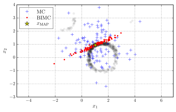
Figure 11: A failure case. Here, $f(\bm{x})=\sin(x_{1})\cos(x_{2})$ is a periodic function in $\mathbb{R}^{2}$. Gray markers depict samples from the ideal IS density $q^{*}$ in this case.

Summary

In summary, the effectiveness of BIMC depends on the interplay between the directions not informed by the pseudo-data point, and the variation of the forward map in these directions. If, at the scale of the covariance of the nominal density $p$, $f(\bm{x})$ varies too quickly in these directions (like the Periodic example), the PDF constructed in BIMC will make for a poor IS density. On the other hand, if $f(\bm{x})$ varies slowly enough (as in the synthetic non-linear, and autoignition examples) or not at all (the affine case), then BIMC is effective. Thus, we conclude that BIMC is best suited to forward maps that are weakly non-linear at the scale of the covariance of the nominal density $p$. Physically, this means that the uncertainties in the input parameters must small enough that $f$ appears almost linear. Note that $f$ can still be highly non-linear at larger scales.

Apart from the forward map being only weakly non-linear, there are two additional requirements. The regions in parameter space that evaluate inside $\mathbb{Y}$ should not be disjoint. The final and perhaps the most important requirement is that the solution of the inverse problem must be computable.

5 Conclusion and future work

In this article, we addressed the problem of efficiently computing rare-event probabilities in systems with uncertain input parameters. Our approach, called BIMC, employs importance sampling in order to achieve efficiency. Noting the structural similarity between the (theoretical) ideal importance sampling density and the posterior distribution of a fictitious inference problem, our importance sampling distribution is constructed by approximating such a fictitious posterior via a Gaussian distribution. The approximation process allows the incorporation of the derivatives of the input-output map into the importance sampling distribution, which is how our scheme achieves parsimonious sampling. Our theoretical analysis establishes that this procedure is optimal in the setting where the input-output map is affine and the nominal density is Gaussian. Hence, BIMC is best applied to maps that appear nearly affine at the scale of the covariance of the nominal distribution. Our numerical experiments support this conclusion and demonstrate that when this is the case, BIMC can lead to speedups of several orders-of-magnitude. Experiments also reveal several drawbacks in BIMC. We will concern ourselves with fixing these drawbacks in part II of this paper.

References

- [1] V. Akçelik, G. Biros, O. Ghattas, J. Hill, D. Keyes, and B. van Bloemen Waanders, Parallel algorithms for PDE-constrained optimization, in Parallel Processing for Scientific Computing, SIAM, 2006, pp. 291–322.
- [2] S. Au and J. Beck, A new adaptive importance sampling scheme for reliability calculations, Structural Safety, 21 (1999), pp. 135 – 158, https://doi.org/https://doi.org/10.1016/S0167-4730(99)00014-4, http://www.sciencedirect.com/science/article/pii/S0167473099000144.
- [3] S. Au, C. Papadimitriou, and J. Beck, Reliability of uncertain dynamical systems with multiple design points, Structural Safety, 21 (1999), pp. 113 – 133, https://doi.org/https://doi.org/10.1016/S0167-4730(99)00009-0, http://www.sciencedirect.com/science/article/pii/S0167473099000090.
- [4] S.-K. Au and J. L. Beck, Estimation of small failure probabilities in high dimensions by subset simulation, Probabilistic Engineering Mechanics, 16 (2001), pp. 263 – 277, https://doi.org/https://doi.org/10.1016/S0266-8920(01)00019-4, http://www.sciencedirect.com/science/article/pii/S0266892001000194.
- [5] J. Breidt, T. Butler, and D. Estep, A measure-theoretic computational method for inverse sensitivity problems I: Method and analysis, SIAM Journal on Numerical Analysis, 49 (2011), pp. 1836–1859, https://doi.org/10.1137/100785946, https://doi.org/10.1137/100785946, https://arxiv.org/abs/https://doi.org/10.1137/100785946.
- [6] C. G. Bucher, Adaptive sampling - an iterative fast monte carlo procedure, Structural Safety, 5 (1988), pp. 119 – 126, https://doi.org/https://doi.org/10.1016/0167-4730(88)90020-3, http://www.sciencedirect.com/science/article/pii/0167473088900203.
- [7] T. Butler, D. Estep, and J. Sandelin, A computational measure theoretic approach to inverse sensitivity problems II: A posteriori error analysis, SIAM Journal on Numerical Analysis, 50 (2012), pp. 22–45, https://doi.org/10.1137/100785958, https://doi.org/10.1137/100785958, https://arxiv.org/abs/https://doi.org/10.1137/100785958.
- [8] P.-T. De Boer, D. P. Kroese, S. Mannor, and R. Y. Rubinstein, A tutorial on the cross-entropy method, Annals of Operations Research, 134 (2005), pp. 19–67.
- [9] M. Fasiolo, F. E. de Melo, and S. Maskell, Langevin incremental mixture importance sampling, Statistics and Computing, 28 (2018), pp. 549–561.
- [10] M. Gunzburger, Perspectives in Flow Control and Optimization, Society for Industrial and Applied Mathematics, 2002, https://doi.org/10.1137/1.9780898718720, https://epubs.siam.org/doi/abs/10.1137/1.9780898718720, https://arxiv.org/abs/https://epubs.siam.org/doi/pdf/10.1137/1.9780898718720.
- [11] J. R. Hershey and P. A. Olsen, Approximating the Kullback Leibler Divergence Between Gaussian Mixture Models, in 2007 IEEE International Conference on Acoustics, Speech and Signal Processing - ICASSP ’07, vol. 4, April 2007, pp. IV–317–IV–320, https://doi.org/10.1109/ICASSP.2007.366913.
- [12] T. Isaac, N. Petra, G. Stadler, and O. Ghattas, Scalable and efficient algorithms for the propagation of uncertainty from data through inference to prediction for large-scale problems, with application to flow of the antarctic ice sheet, Journal of Computational Physics, 296 (2015), pp. 348 – 368, https://doi.org/https://doi.org/10.1016/j.jcp.2015.04.047, http://www.sciencedirect.com/science/article/pii/S0021999115003046.
- [13] H. Kahn and A. W. Marshall, Methods of reducing sample size in Monte Carlo computations, Journal of the Operations Research Society of America, 1 (1953), pp. 263–278.
- [14] L. Katafygiotis and K. Zuev, Estimation of small failure probabilities in high dimensions by adaptive linked importance sampling, COMPDYN 2007, (2007).
- [15] B. Kramer, A. N. Marques, B. Peherstorfer, U. Villa, and K. Willcox, Multifidelity probability estimation via fusion of estimators, Tech. Report ACDL TR-2017-3, Massachusetts Institute of Technology, 2017.
- [16] C. Lieberman and K. Willcox, Goal-oriented inference: Approach, linear theory, and application to advection diffusion, SIAM Review, 55 (2013), pp. 493–519, https://doi.org/10.1137/130913110, https://doi.org/10.1137/130913110, https://arxiv.org/abs/https://doi.org/10.1137/130913110.
- [17] C. Lieberman and K. Willcox, Nonlinear goal-oriented Bayesian inference: Application to carbon capture and storage, SIAM Journal on Scientific Computing, 36 (2014), pp. B427–B449.
- [18] E. N. Lorenz, Deterministic nonperiodic flow, Journal of the Atmospheric Sciences, 20 (1963), pp. 130–141.
- [19] R. Melchers, Importance sampling in structural systems, Structural Safety, 6 (1989), pp. 3 – 10, https://doi.org/https://doi.org/10.1016/0167-4730(89)90003-9, http://www.sciencedirect.com/science/article/pii/0167473089900039.
- [20] A. B. Owen, Monte Carlo theory, methods and examples, 2013.
- [21] B. Peherstorfer, T. Cui, Y. Marzouk, and K. Willcox, Multifidelity importance sampling, Computer Methods in Applied Mechanics and Engineering, 300 (2016), pp. 490 – 509, https://doi.org/http://dx.doi.org/10.1016/j.cma.2015.12.002, http://www.sciencedirect.com/science/article/pii/S004578251500393X.
- [22] B. Peherstorfer, B. Kramer, and K. Willcox, Multifidelity preconditioning of the cross-entropy method for rare event simulation and failure probability estimation, SIAM/ASA Journal on Uncertainty Quantification, (2018).
- [23] R. Rackwitz, Reliability analysis - a review and some perspectives, Structural Safety, 23 (2001), pp. 365 – 395, https://doi.org/https://doi.org/10.1016/S0167-4730(02)00009-7, http://www.sciencedirect.com/science/article/pii/S0167473002000097.
- [24] A. E. Raftery and L. Bao, Estimating and projecting trends in HIV/AIDS generalized epidemics using incremental mixture importance sampling, Biometrics, 66 (2010), pp. 1162–1173.
- [25] C. P. Robert and G. Casella, Monte Carlo Integration, Springer New York, New York, NY, 2004, pp. 79–122, https://doi.org/10.1007/978-1-4757-4145-2_3, http://dx.doi.org/10.1007/978-1-4757-4145-2_3.
- [26] G. Rubino and B. Tuffin, Rare event simulation using Monte Carlo methods, John Wiley & Sons, 2009.
- [27] G. Schuëller and R. Stix, A critical appraisal of methods to determine failure probabilities, Structural Safety, 4 (1987), pp. 293 – 309, https://doi.org/https://doi.org/10.1016/0167-4730(87)90004-X, http://www.sciencedirect.com/science/article/pii/016747308790004X.
- [28] A. Spantini, T. Cui, K. Willcox, L. Tenorio, and Y. Marzouk, Goal-oriented optimal approximations of Bayesian linear inverse problems, SIAM Journal on Scientific Computing, 39 (2017), pp. S167–S196, https://doi.org/10.1137/16M1082123, https://doi.org/10.1137/16M1082123, https://arxiv.org/abs/https://doi.org/10.1137/16M1082123.
- [29] U. Villa, N. Petra, and O. Ghattas, hIPPYlib: an Extensible Software Framework for Large-Scale Deterministic and Bayesian Inverse Problems, Journal of Open Source Software, 3 (2018), https://doi.org/10.21105/joss.00940.
- [30] U. Villa, N. Petra, and O. Ghattas, hIPPYlib: An Extensible Software Framework for Large-Scale Inverse Problems Governed by PDEs; Part I: Deterministic Inversion and Linearized Bayesian Inference, arXiv e-prints, (2019), https://arxiv.org/abs/1909.03948.