Viability of Bouncing Cosmology in Energy-Momentum-Squared Gravity

Abstract

We analyze the early-time isotropic cosmology in the so-called energy-momentum-squared gravity (EMSG). In this theory, a $T_{\mu\nu}T^{\mu\nu}$ term is added to the Einstein-Hilbert action, which has been shown to replace the initial singularity by a regular bounce. We show that this is not the case, and the bouncing solution obtained does not describe our Universe since it belongs to a different solution branch. The solution branch that corresponds to our Universe, while nonsingular, is geodesically incomplete. We analyze the conditions for having viable regular-bouncing solutions in a general class of theories that modify gravity by adding higher order matter terms. Applying these conditions on generalizations of EMSG that add a $\left(T_{\mu\nu}T^{\mu\nu}\right)^{n}$ term to the action, we show that the case of $n=5/8$ is the only one that can give a viable bouncing solution, while the $n>5/8$ cases suffer from the same problem as EMSG, i.e. they give nonsingular, geodesically incomplete solutions. Furthermore, we show that the $1/2<n<5/8$ cases can provide a nonsingular initially de Sitter solution. Finally, the expanding, geodesically incomplete branch of EMSG or its generalizations can be combined with its contracting counterpart using junction conditions to provide a (weakly) singular bouncing solution. We outline the junction conditions needed for this extension and provide the extended solution explicitly for EMSG. In this sense, EMSG replaces the standard early-time singularity by a singular bounce instead of a regular one.

I Introduction

Recent cosmological observations provided us with strong evidence for the accelerating expansion of the Universe Riess et al. (1998); Ade et al. (Planck Collaboration). Trying to understand this acceleration in general relativity (GR) one is led to two possibilities: exotic matter content or a cosmological constant ($\Lambda$). Although these possibilities can fit the observational data, they do not provide us with a fundamental explanation of this acceleration. In addition to this large scale problem, GR predicts its own doom at small scales through the occurrence of spacetime singularities Hawking and Penrose (1970), which are expected to be cured in a full theory of quantum gravity (or at least an effective approximation of it). These issues have led to a plethora of modified-gravity theories (see Clifton et al. (2012); Nojiri et al. (2017) for a review, and also Ishak (2019) for a review on the recent observational constraints). In these theories, GR is seen as an effective field theory (of a more general gravitational theory) that might get corrections either at very large or very small scales.

Some of these modified theories have been shown to replace the initial cosmological singularity that occurs in GR by a regular bounce (see Novello and Bergliaffa (2008); Battefeld and Peter (2015) for a review). Along these efforts, energy-momentum-squared gravity (EMSG), as dubbed by its original authors, was proposed in Roshan and Shojai (2016). This theory modifies gravity by adding a $T_{\mu\nu}T^{\mu\nu}$ term to the Einstein-Hilbert Lagrangian; it is a special case of theories that have a Lagrangian of the form $f(R,T_{\mu\nu}T^{\mu\nu})$ which were first studied in Katırcı and Kavuk (2014).

Further efforts were conducted to study generalizations of EMSG and their implications. Various cosmological models of higher order generalizations of EMSG, which add terms in the form $\left(T_{\mu\nu}T^{\mu\nu}\right)^{n}$, were considered in Board and Barrow (2017) particularly for the case $n>1/2$ relevant to high density scales, while the case $n<1/2$ relevant to late time cosmology was studied in Akarsu et al. (2018a). The cosmological implications for the case $n=1/2$ were studied in Akarsu et al. (2018b), which is interesting since the coupling in this case becomes dimensionless. Besides the form $\left(T_{\mu\nu}T^{\mu\nu}\right)^{n}$, a logarithmic generalization, dubbed as energy-momentum log gravity (EMLG), was considered in Akarsu et al. (2019) where the term $\ln{(\lambda T_{\mu\nu}T^{\mu\nu})}$ was used to extend the $\Lambda$CDM model to study viable cosmologies and to address the tension in $H_{0}$ measurements. Furthermore, phenomenological investigations were done in Akarsu et al. (2018c) using observational data from neutron stars to constrain the free parameter in EMSG, while in Faria et al. (2019) low redshift data were used to constrain $\left(T_{\mu\nu}T^{\mu\nu}\right)^{n}$ theories. In addition to these studies, linear stability analysis was used in Bahamonde et al. (2019) to investigate two models in $f(R,T_{\mu\nu}T^{\mu\nu})$ .

In this study, we focus on the analysis of the early-time cosmological behavior of EMSG and its generalizations, particularly regarding the existence of regular bounces in this class of theories. As a result, we show that the bounce obtained in Roshan and Shojai (2016) is not viable, and that generic theories that modify GR by adding higher order matter terms cannot provide a viable regular bounce.

The structure of this paper is as follows. In Sec. II, we review the EMSG theory and its field equations. In Sec. III, we analyze the isotropic early-time cosmology of EMSG showing that the bounce obtained in Roshan and Shojai (2016) is not viable. We show that the correct solution-branch corresponding to our Universe is also nonsingular but is not valid beyond a certain point in time, i.e. past-geodesically incomplete. In Sec. IV, we analyze the conditions for having a viable bounce in theories that modify gravity by adding higher order matter terms. We apply these conditions to $\left(T_{\mu\nu}T^{\mu\nu}\right)^{n}$ generalizations of EMSG. In Sec. V, we outline the junction conditions needed for extending the geodesically incomplete solutions of EMSG and similar theories. Finally, we conclude with summary and discussion of the results in Sec. VI.

II Energy-Momentum-Squared Gravity

The EMSG action can be written as

$$S_{\text{EMSG}}=\int d^{4}x\,\sqrt{-g}\,\left(\frac{1}{2\kappa}R-\frac{\Lambda}{\kappa}-\frac{1}{2}\alpha\,T_{\mu\nu}T^{\mu\nu}\right)+S_{\text{M}}\,,$$ (1)

where $\kappa=8\pi G$, $R$ is the Ricci scalar, $\Lambda$ is the cosmological constant and $S_{\text{M}}\equiv\int d^{4}x\,\sqrt{-g}\,L_{m}$ with $L_{m}$ as the matter Lagrangian density. Here and thereafter, we use units where $c=1$ and the metric signature $(-,+,+,+)$.

The extra term that makes this theory different from GR is $-\frac{1}{2}\alpha\,T_{\mu\nu}T^{\mu\nu}$, where $\alpha$ is a free parameter in the theory (with dimensions of inverse energy-density) which can be constrained from observations as was done in Akarsu et al. (2018c), and $T_{\mu\nu}$ is the ordinary energy-momentum tensor defined as

$$T_{\mu\nu}=-\frac{2}{\sqrt{-g}}\frac{\delta\left(\sqrt{-g}L_{m}\right)}{\delta g^{\mu\nu}}.$$ (2)

The factor of $-\frac{1}{2}$, while it can be absorbed into the definition of $\alpha$ , is retained here for convenience. In this case $\alpha$ can be matched with $\frac{\eta}{\kappa}$ in the original paper Roshan and Shojai (2016) where $\eta$ was the free parameter in that case. While $\alpha$ could be positive or negative, we will restrict ourselves to the $\alpha>0$ case since it has been shown to give a more interesting behavior in early-time cosmology Roshan and Shojai (2016).

Now that we have introduced the action of EMSG, let us turn to the question of how this action can be defined in the first place; that is, how does the total action already contain the energy-momentum tensor which is defined by varying part of the total action (i.e. $S_{\text{M}}$)? The main argument in Roshan and Shojai (2016); Nari and Roshan (2018) is that one does not have to know anything about the gravitational theory beforehand in order to define the energy-momentum tensor, one only needs matter physical variables, or simply: the matter Lagrangian density $L_{m}$. In other words, there is a well-defined way to construct $T_{\mu\nu}$ in a given theory without gravity, and the $T_{\mu\nu}T^{\mu\nu}$ term (which is just a scalar function in the fields, their derivatives and the metric) is added as a form of nonminimal coupling of that theory to gravity.

EMSG is characterized by a density scale $\alpha^{-1}$; deviations from GR should start appearing near that scale. Since the theory has a characteristic density scale rather than an energy scale, one can construct a length scale for physical solutions that have a specific energy scale. For example, for a charged black hole with a charge $q$, a characteristic length scale would be $\ell\sim\left(\alpha q^{2}\right)^{1/4}$, which is the length scale at which the electromagnetic energy density would be comparable to $\alpha^{-1}$. The physical relevance of that length can be solution dependent, but the interesting part is that if the dynamics of the theory impose a maximum density $\sim\alpha^{-1}$, we get a minimum length $\sim\ell$.

Let us now turn to the field equations. EMSG is equivalent to GR coupled to an effective matter Lagrangian; therefore the field equations are just the Einstein equations but sourced by an effective energy-momentum tensor, and so we have

$$G_{\mu\nu}+\Lambda g_{\mu\nu}=\kappa T_{\mu\nu}^{\text{eff}},$$ (3)

where

$$T_{\mu\nu}^{\text{eff}}=T_{\mu\nu}-\frac{1}{2}\alpha T_{\sigma\rho}T^{\sigma\rho}g_{\mu\nu}+\alpha\Theta_{\mu\nu},$$ (4)

and

$$\Theta_{\mu\nu}\equiv\frac{\delta\left(T_{\sigma\rho}T^{\sigma\rho}\right)}{\delta g^{\mu\nu}}=2T_{\mu\sigma}T_{\,\,\nu}^{\sigma}-2L_{m}\left(T_{\mu\nu}-\frac{1}{2}Tg_{\mu\nu}\right)-TT_{\mu\nu}-4T^{\sigma\rho}\frac{\partial^{2}L_{m}}{\partial g^{\mu\nu}\partial g^{\sigma\rho}}.$$ (5)

The details of variation of the extra term can be found in Appendix A.

III Cosmology in EMSG

Let us start by taking a closer look at the early time cosmology in EMSG, which was studied in Roshan and Shojai (2016); Akarsu et al. (2018c). We will work with a flat Friedmann-Robertson-Walker (FRW) metric $ds^{2}=-dt^{2}+a(t)^{2}\delta_{ij}dx^{i}dx^{j}$. We will also assume a small positive cosmological constant as in the usual $\Lambda$CDM model. Assuming a perfect fluid content, we have

$$T_{\mu\nu}=(\rho+p)\,u_{\mu}u_{\nu}+p\,g_{\mu\nu},$$ (6)

where $\rho$ is the energy density, $p$ is the pressure and $u^{\mu}$ is the four-velocity of the fluid, which satisfies the conditions $u^{\mu}u_{\mu}=-1$ and $\nabla_{\nu}\left(u^{\mu}u_{\mu}\right)=0$. We can arrive at the perfect-fluid energy-momentum tensor through different Lagrangian densities ($L_{m}=p$ or $L_{m}=-\rho$), which does not pose a problem in GR Schutz (1970); *Brown_1993_fluid_lagrangian. However, in EMSG the Lagrangian density appears explicitly in the field equations and thus the choice of the Lagrangian density affects the dynamics. While there is no consensus on which Lagrangian to use (see Bertolami et al. (2008); *Faroni2009_perfect_fluid for a detailed discussion), we will stick to the choice of $L_{m}=p$ to follow with the EMSG literature.

For a perfect fluid with $L_{m}=p$, the effective energy momentum tensor sourcing gravity can be written as

$$T_{\mu\nu}^{\text{eff}}=(\rho_{\text{eff}}+p_{\text{eff}})\,u_{\mu}u_{\nu}+p_{\text{eff}}\,g_{\mu\nu}.$$ (7)

where

$$\rho_{\text{eff}}=\rho-\frac{1}{2}\alpha\left(3p^{2}+8p\rho+\rho^{2}\right),$$ (8)

$$p_{\text{eff}}=p-\frac{1}{2}\alpha\left(3p^{2}+\rho^{2}\right).$$ (9)

The effective density and pressure can be defined covariantly as

$$\rho_{\text{eff}} \coloneqq u^{\mu}u^{\nu}T_{\mu\nu}^{\text{eff}},$$ (10)

$$p_{\text{eff}} \coloneqq\frac{1}{3}\left(g^{\mu\nu}+u^{\mu}u^{\nu}\right)T_{\mu\nu}^{\text{eff}}.$$ (11)

The Friedmann equations are the same as in GR but with the density and pressure replaced by their effective counterparts, thus we have

$$H^{2}=\frac{\Lambda}{3}+\frac{\kappa}{3}\rho_{\text{eff}},$$ (12)

$$\frac{\ddot{a}}{a}=\dot{H}+H^{2}=\frac{\Lambda}{3}-\frac{\kappa}{6}\left(\rho_{\text{eff}}+3p_{\text{eff}}\right).$$ (13)

The remaining equation is the fluid conservation/continuity equation, which comes from $\nabla^{\mu}T_{\mu\nu}^{\text{eff}}=0$, and of course can be obtained from the above two equations. Again, this is nothing more than the fluid conservation equation in GR with the effective density and pressure, thus we have

$$\dot{\rho}_{\text{eff}}+3\frac{\dot{a}}{a}\left(\rho_{\text{eff}}+p_{\text{eff}}\right)=0,$$ (14)

which can be cast into an autonomous form as

$$\rho_{\text{eff}}^{{}^{\prime}}+3\left(\rho_{\text{eff}}+p_{\text{eff}}\right)=0,$$ (15)

where the prime denotes derivative with respect to $\ln a$ .

III.1 Two-component fluids

Before we attempt to solve the equations, it is worth noting that because the effective density and pressure are nonlinear in the ordinary density and pressure, dealing with a multicomponent fluid here will be drastically different than in GR. In particular, the conservation equation (15) will lead to one equation for both fluids. If we have a two-component fluid, with each component having a barotropic equation of state in the form $p=\omega\rho$, then the conservation equation (15) becomes

$$\left[1-\alpha\left(4\omega_{1}+3\omega_{1}\omega_{2}+4\omega_{2}+1\right)\rho_{2}-\alpha\left(3\omega_{1}^{2}+8\omega_{1}+1\right)\rho_{1}\right]\rho_{1}^{\prime}$$

$$+\left[1-\alpha\left(4\omega_{1}+3\omega_{1}\omega_{2}+4\omega_{2}+1\right)\rho_{1}-\alpha\left(3\omega_{2}^{2}+8\omega_{2}+1\right)\rho_{2}\right]\rho_{2}^{\prime}$$

$$+3\left(\omega_{1}+1\right)\rho_{1}-3\alpha\left(3\omega_{1}^{2}+4\omega_{1}+1\right)\rho_{1}^{2}$$

$$+3\left(\omega_{2}+1\right)\rho_{2}-3\alpha\left(3\omega_{2}^{2}+4\omega_{2}+1\right)\rho_{2}^{2}$$

$$-6\alpha\left(2\omega_{1}+3\omega_{1}\omega_{2}+2\omega_{2}+1\right)\rho_{1}\rho_{2}\,\,\, =0.$$ (16)

This is one equation for both components, but we should have individual equations of motion for each component. Just like for cases other than perfect fluids, each field has its own equation of motion, and the conservation of the total energy momentum tensor is satisfied automatically on shell, i.e. it gives a sum of terms where each term vanishes on its own when the respective equation of motion is satisfied. The problem with fluids is that we do not get the continuity or the Euler equations for each fluid component directly through variation of the action ; instead, we get those equations for the two fluids combined from the conservation of the total energy-momentum tensor. Thus, for a two-component fluid, we should expect to be able to split the conservation equation into two equations: one equation for each component. In GR, the split is straightforward since the conservation equation there is linear; in our case, the splitting seems rather to be an ambiguous task. We can break this ambiguity using the fact that the Lagrangian is invariant under exchange of component labels, i.e. $\rho_{1}\longleftrightarrow\rho_{2}$ and $p_{1}\longleftrightarrow p_{2}$. Given this symmetry, we should expect that the individual-component equations are mapped to one another under the exchange of labels. Applying this argument on (16), the individual equations for components 1 and 2 respectively are

$$\left[1-\alpha\left(4\omega_{1}+3\omega_{1}\omega_{2}+4\omega_{2}+1\right)\rho_{2}-\alpha\left(3\omega_{1}^{2}+8\omega_{1}+1\right)\rho_{1}\right]\rho_{1}^{\prime}$$

$$+3\left(\omega_{1}+1\right)\rho_{1}-3\alpha\left(3\omega_{1}^{2}+4\omega_{1}+1\right)\rho_{1}^{2}$$

$$-3\alpha\left(2\omega_{1}+3\omega_{1}\omega_{2}+2\omega_{2}+1\right)\rho_{1}\rho_{2}\,\,\, =0,$$ (17)

$$\left[1-\alpha\left(4\omega_{1}+3\omega_{1}\omega_{2}+4\omega_{2}+1\right)\rho_{1}-\alpha\left(3\omega_{2}^{2}+8\omega_{2}+1\right)\rho_{2}\right]\rho_{2}^{\prime}$$

$$+3\left(\omega_{2}+1\right)\rho_{2}-3\alpha\left(3\omega_{2}^{2}+4\omega_{2}+1\right)\rho_{2}^{2}$$

$$-3\alpha\left(2\omega_{1}+3\omega_{1}\omega_{2}+2\omega_{2}+1\right)\rho_{1}\rho_{2}\,\,\, =0,$$ (18)

which are interchanged under $\rho_{1}\longleftrightarrow\rho_{2}$ and $\omega_{1}\longleftrightarrow\omega_{2}$. This result can be easily generalized to the case of an $n$-component fluid by noting that the Lagrangian then would be invariant under the interchange of the labels of each pair of components, and the fact that the interaction terms will still be quadratic in the densities. Thus, the equation for the $i$th component in that case would be

$$\left(1-\alpha\left(3\omega_{i}^{2}+8\omega_{i}+1\right)\rho_{i}\right)\rho_{i}^{\prime}+3\left(\omega_{i}+1\right)\rho_{i}-3\alpha\left(3\omega_{i}^{2}+4\omega_{i}+1\right)\rho_{i}^{2}$$

$$-\alpha\sum_{j\neq i}^{n}\left\{\left(4\omega_{i}+3\omega_{i}\omega_{j}+4\omega_{j}+1\right)\rho_{j}\rho_{i}^{\prime}\right.$$

$$\left.+3\left(2\omega_{i}+3\omega_{i}\omega_{j}+2\omega_{j}+1\right)\rho_{i}\rho_{j}\right\}\,\, =0.$$ (19)

Now that we have an equation of motion for each fluid component, it is important to note that these equations are the ones that determine how the fluid density of each component behaves with the scale $a$. For example, in GR the solutions for matter and radiation are $\rho_{m}\sim a^{-3}$ and $\rho_{r}\sim a^{-4}$, which tells us that radiation is the dominant component in the early Universe where $a$ is very small. In our case, we need to solve Eqs. (17) and (18) simultaneously for matter and radiation content, which can be quite difficult analytically without resorting to some kind of approximation. In Appendix B, we show that indeed radiation will be dominant in the early Universe in EMSG.

III.2 Radiation domination

Before focusing on radiation, let us start by considering a general one-component fluid in EMSG. In what follows, although $\Lambda$ can be ignored since we are interested only in the early Universe, we will keep it for reasons to be clear shortly.

For a one-component fluid with a barotropic equation of state of the form $p=\omega\rho$, the effective density and pressure in (8) and (9) become

$$\rho_{\text{eff}}=\rho-\frac{1}{2}\left(3\omega^{2}+8\omega+1\right)\alpha\rho^{2},$$ (20)

$$p_{\text{eff}}=\omega\rho-\frac{1}{2}\left(3\omega^{2}+1\right)\alpha\rho^{2}.$$ (21)

At this point it is worth noting that one can find values for $\omega$ such that the effective equation of state maintains the same form as the original equation of state, i.e. $p_{\text{eff}}=\omega\rho_{\text{eff}}.$ It is easy to see from (20) and (21) that these special values for $\omega$ satisfy the following cubic equation:

$$3\omega^{2}+1=\omega\left(3\omega^{2}+8\omega+1\right).$$ (22)

This gives the solutions $\omega=-1$ and $\omega=1/3$ ($\omega=-1$ is a repeated root). Given this result, it would be interesting to consider a dark energy ($\omega=-1$) fluid in EMSG, but in this paper we will concern ourselves with a $\Lambda$CDM-like model in EMSG with nonexotic fluids (i.e. only matter and radiation). We note that these specific values for $\omega$ that preserve the equation of state are nothing but a coincidence in EMSG, and other values (if any) would appear in higher order generalizations.

In general, $p_{\text{eff}}$ is not always single valued in $\rho_{\text{eff}}$; this is due to the fact that (20) is not invertible over the entire domain of $\rho$; however, we can put it in the form $p_{\text{eff}}=\omega_{\text{eff}}(\rho)\,\rho_{\text{eff}}$ by dividing (21) by (20) to get $\omega_{\text{eff}}$ as

$$\omega_{\text{eff}}(\rho) =\frac{\omega-\frac{1}{2}\left(3\omega^{2}+1\right)\alpha\rho}{1-\frac{1}{2}\left(3\omega^{2}+8\omega+1\right)\alpha\rho}.$$ (23)

As we can see from (20), for values of $\omega$ that keep $3\omega^{2}+8\omega+1>0$, $\rho_{\text{eff}}$ is not a monotonically increasing function of $\rho$ and can be zero (or even be negative) for $\rho>0$; this feature is what makes this theory appealing, since it opens the possibility of having a critical point $H=0$ at high densities [which can be seen directly from (12)], similar to other theories, like loop quantum gravity Ashtekar et al. (2006); *Bounce_in_LQC_2006 or braneworlds Shtanov and Sahni (2003) that have a Friedmann equation of the form

$$H^{2}\sim\rho(1-\frac{\rho}{\rho_{\text{critical}}}),$$ (24)

where in EMSG $\rho_{\text{critical}}$ would be $O(\alpha^{-1})$.

If we look for a critical point $H=0$ in EMSG, we will need [from (12)] to have $\rho_{\text{eff}}=-\frac{\Lambda}{\kappa}$, which from (20) gives the critical density as

$$\rho_{\text{critical}}=\frac{1+\sqrt{1+2\alpha\frac{\Lambda}{\kappa}\left(3\omega^{2}+8\omega+1\right)}}{\alpha\left(3\omega^{2}+8\omega+1\right)},$$ (25)

where we have discarded the other solution as it leads to $\rho\simeq-\frac{\Lambda}{\kappa}+O\left(\frac{\alpha\Lambda^{2}}{\kappa^{2}}\right)$. At the critical density, using the expressions for $\rho_{\text{eff}}$ and $p_{\text{eff}}$ in (20) and (21), the acceleration equation (13) becomes

$$\frac{\ddot{a}}{a}=\dot{H}=\frac{(\omega+1)(3\omega+1)}{(3\omega^{2}+8\omega+1)}\Lambda-\frac{\kappa(\omega+1)^{2}(3\omega-1)}{2\alpha(3\omega^{2}+8\omega+1)^{2}}\left(1+\sqrt{1+2\alpha\frac{\Lambda}{\kappa}\left(3\omega^{2}+8\omega+1\right)}\right).$$ (26)

It is easy to check, given that we expect $\alpha^{-1}\ggg\frac{\Lambda}{\kappa}$ , that $\dot{H}<0$ for $\omega>1/3$ as the second term in (26) dominates and it is negative for those values of $\omega$. Therefore, the critical point we found corresponds to a bounce only for $\omega\leq 1/3$.

III.2.1 Bounce point and its viability

Let us now turn our attention to radiation ($\omega=1/3$), which has an effective density and pressure as

$$\rho_{\text{eff}} =\rho_{r}-2\alpha\rho_{r}^{2},$$ (27)

$$p_{\text{eff}} =\frac{\rho_{r}}{3}-\frac{2\alpha\rho_{r}^{2}}{3}.$$ (28)

At the critical point, from (25), the radiation density will be

$$\rho_{r\,\text{crit.}}=\frac{1}{4\alpha}\left(1+\sqrt{1+8\alpha\frac{\Lambda}{\kappa}}\right),$$ (29)

and as we see from (26), this gives $\dot{H}=\frac{2\Lambda}{3}$. This was the main reason of keeping $\Lambda$ explicit up until this point, to show that we can get $\dot{H}>0$ at the critical point due to $\Lambda>0$, which was an argument in Roshan and Shojai (2016) for the necessity of having a positive cosmological constant in this theory. It is worth noting, however, that if we had not ignored the matter fluid component, it could have led to a similar result, i.e. $\dot{H}\sim\rho_{m}>0$ without the need for any cosmological constant. In either case, one can conclude that the point at which the density is as in (29) corresponds to a regular bounce as was concluded in Roshan and Shojai (2016). However, we will show that this critical point does not correspond to a solution that describes our Universe. To see this, let us solve the conservation equation explicitly. From (27), (28) and (15), we get the conservation equation for radiation as

$$\left(1-4\alpha\rho_{r}\right)\rho_{r}^{\prime}+4\rho_{r}-8\alpha\rho_{r}^{2}=0.$$ (30)

Notice that this ordinary differential equation (ODE) has a regular singular point at $\rho_{r}=\frac{1}{4\alpha}$, we will discuss the relevance of this issue later. Since this is an autonomous ODE with respect to $\ln a$ , it can be integrated directly to give $\ln a$ as a function of $\rho_{r}$ . Integrating with the condition $a(\rho_{r0})=a_{0}$, where $\rho_{r0}$ is the cosmological radiation density at the present time , and setting $a_{0}=1$, we get

$$a=\left(\frac{\rho_{r0}\left(1-2\alpha\rho_{r0}\right)}{\rho_{r}\left(1-2\alpha\rho_{r}\right)}\right)^{1/4}.$$ (31)

This expression reduces to the usual $a=\left(\frac{\rho_{r0}}{\rho_{r}}\right)^{1/4}$ for low densities (i.e. in the limit $\alpha\rho_{r}\rightarrow 0$). Since $a$ has to be real, we must have

$$\rho_{r}<\frac{1}{2\alpha}.$$ (32)

Notice that having $\rho_{r0}<\frac{1}{2\alpha}$ is the main cause of this constraint. The density at the critical point in (29) clearly violates (32), and thus the critical point is unphysical and there is no bouncing solution that corresponds to our Universe. In a hypothetical universe where $\rho_{r0}>\frac{1}{2\alpha}$, the requirement that $a$ has to be real would have led instead to $\rho_{r}>\frac{1}{2\alpha}$, and the critical point (29) would have corresponded indeed to a bouncing solution in that universe. In other words, EMSG gives a valid regular bounce in a universe where the density is always higher than $\frac{1}{2\alpha}$.

III.2.2 Radiation domination solution

Solving for $\rho_{r}$ in (31), we get

$$\rho_{r}(a)=\frac{1}{4\alpha}\left(1\pm\sqrt{1-8\alpha\rho_{r0}\left(1-2\alpha\rho_{r0}\right)a^{-4}}\right).$$ (33)

We pick the negative branch because it gives the asymptotic behavior of $\rho_{r}\simeq\rho_{r0}a^{-4}$ for relatively large $a$. Since we want $\rho_{r}$ to be real, we must have a maximum density $\rho_{r\,\text{max}}=\frac{1}{4\alpha}$ corresponding to a minimum scale factor. We can then write the solution as

$$\rho_{r}(a)=\frac{1}{4\alpha}\left(1-\sqrt{1-\left(\frac{a_{\text{min}}}{a}\right)^{4}}\right),$$ (34)

where

$$a_{\text{min}}\equiv\left(8\alpha\rho_{r0}\left(1-2\alpha\rho_{r0}\right)\right)^{1/4}.$$ (35)

The existence of a minimum scale factor here comes from the constraint $\rho_{r}\in\mathbb{R}$ rather than from the dynamical solution $a(t)$ as in the case of a bounce; this will lead to geodesic incompletion as we will see shortly. One can easily get $a(t)$ by plugging (34) in the Friedmann equation (12). An equivalent, but clearer, way is to notice that since $p_{\text{eff}}=\frac{1}{3}\rho_{\text{eff}}$, the conservation equation (15) becomes

$$\rho_{\text{eff}}^{{}^{\prime}}+4\rho_{\text{eff}}=0;$$ (36)

we can solve this with the already known condition that $\rho_{r}(a_{\text{min}})=\frac{1}{4\alpha}$, which gives us $\rho_{\text{eff}}(a_{\text{min}})=\frac{1}{8\alpha}$. With the latter condition, we get the solution

$$\rho_{\text{eff}}(a)=\frac{1}{8\alpha}\left(\frac{a_{\text{min}}}{a}\right)^{4}.$$ (37)

Plugging (37) in the Friedmann equation (12), we get

$$H^{2}=\frac{\Lambda}{3}+\frac{\kappa}{24\alpha}\left(\frac{a_{\text{min}}}{a}\right)^{4}.$$ (38)

We can clearly see now that there are no $H=0$ critical points for all real (physical) values of $a$. From now on, for simplicity, we shall ignore the cosmological constant in the early Universe; it has served its purpose now that we have established that the critical point in (29) does not correspond to a bounce. The Friedmann equation now becomes

$$H=\frac{\dot{a}}{a}=\pm\sqrt{\frac{\kappa}{24\alpha}}\left(\frac{a_{\text{min}}}{a}\right)^{2}.$$ (39)

We can conveniently define

$$H_{\text{max}}\equiv H(a_{\text{min}})=\sqrt{\frac{\kappa}{24\alpha}}.$$ (40)

Solving the positive branch of (39) with the condition $a(0)=a_{\text{min}}$, we get

$$a(t)=a_{\text{min}}\sqrt{1+2H_{\text{max}}t},\,\,\,\,\,\,\,t\geq 0.$$ (41)

This solution, which was found in Akarsu et al. (2018c) [albeit with a redefinition of $t$ to match the standard solution of GR at which $a(0)=0$], manifestly cannot be extended for $t<\frac{-1}{2H_{\text{max}}}$, but more importantly, we cannot extend it for $t<0$ since that would lead to $a<a_{\text{min}}$ and then from (34) the radiation density would become nonreal as we discussed before. This solution can be interpreted, in the spirit of effective field theory, as EMSG breaking down as we approach $a_{\text{min}}$ and one would need new physics to describe what is happening beyond that point. In this sense, $a_{\text{min}}$ is not interpreted as an absolute minimum scale of nature, but the minimum scale at which EMSG is valid.

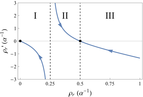
Figure 1: Phase plot for Eq. (30) in units of $\alpha^{-1}$. The dots represent fixed points, while the arrows represent the flow direction in phase space. Region I represents the negative branch of (33), while region II represents the positive branch. Region III contains the bounce point, which is disconnected from the physical region that describes our Universe.

It is interesting to note that while $\dot{\rho_{r}}$ diverges as $t\rightarrow 0$, all geometric quantities [represented by $H(t)$ and its time derivatives] remain finite. This gives us the chance to extend the spacetime beyond $t=0$ by combining the solution in (41) with its counterpart from the negative branch of (39) using junction conditions at $t=0$. We will present this in Sec. V.

We conclude this section by reflecting on the issue that prevented this theory from achieving a cosmologically viable bounce, after all, it had a Friedmann equation reminiscent of theories like loop quantum gravity and braneworlds, so why is the case here different? The reason is that, unlike those theories which modify only the Friedmann equation, EMSG also modifies the conservation/continuity equation. The main issue is that, due to the nonlinearity, the equation is modified in a singular way; particularly, the singular point is at a lower density ($\rho_{r}=\frac{1}{4\alpha}$) than the density at the critical point (29). This causes our Universe to be in a solution-region entirely disconnected from the bounce point; we can see this from the phase plot of the conservation equation (30) in Fig. 1. We note that this problem is not unique to EMSG; it can happen in any other theory that effectively modifies the matter Lagrangian. We discuss the conditions for this issue in the next section.

IV Bounces in More General Theories

Let us start with a more generalized theory than EMSG that effectively modifies the matter Lagrangian but keeps the geometric side as GR, so we would have a total action like

$$S=\int d^{4}x\,\sqrt{-g}\,\left(\frac{1}{2\kappa}R+L_{m\,\text{eff}}\right).$$ (42)

We assume FRW metric and a perfect fluid matter content with a generic equation of state $p=p(\rho)$. We will focus only on a single-component fluid or a fluid with one dominant component in the early Universe (which typically should be the radiation). As in the case with EMSG, the Friedmann equations take the form

$$H^{2}=\frac{\kappa}{3}\rho_{\text{eff}},$$ (43)

$$\dot{H}+H^{2}=-\frac{\kappa}{6}\left(\rho_{\text{eff}}+3p_{\text{eff}}\right).$$ (44)

It is useful to combine these equations to get $\dot{H}$ in terms of $\rho_{\text{eff}}$ and $p_{\text{eff}}$ as

$$\dot{H}=-\frac{\kappa}{2}\left(\rho_{\text{eff}}+p_{\text{eff}}\right).$$ (45)

We have ignored the cosmological constant for simplicity, but the arguments below can be easily generalized by absorbing the cosmological constant in the definition of $\rho_{\text{eff}}$ and $p_{\text{eff}}$. The conservation equation is the same as (14), which can be written in terms of $\dot{\rho}$ as

$$\dot{\rho}=-3H\left(\frac{\rho_{\text{eff}}+p_{\text{eff}}}{\frac{d\rho_{\text{eff}}}{d\rho}}\right).$$ (46)

We want to analyze the conditions at which this theory would give a cosmologically viable regular bounce. From (43), (45) and (46), we see that the behavior of $H$, $\dot{H}$ and $\dot{\rho}$ is controlled by only three functions: $\rho_{\text{eff}}$, $\rho_{\text{eff}}+p_{\text{eff}}$ and $\frac{d\rho_{\text{eff}}}{d\rho}$, which are all functions in $\rho$. So we can take $\rho$ as the basic variable that controls the phase space of this dynamical system. We assume for simplicity that these functions do not have more than one nontrivial zero; the arguments in this section can be generalized otherwise. We also assume that these functions are continuous and smooth as functions of $\rho$; this assumption is important in order to avoid curvature-singularity problems at finite values of $\rho$.

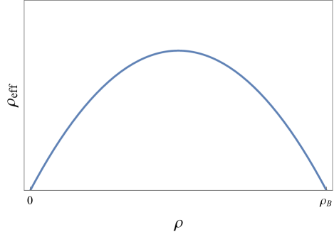
Figure 2: An example profile for the effective density as a function of the ordinary density $\rho$.

IV.1 Bounce analysis

In order for this theory to have a bounce at some high density $\rho_{\text{B}}$, the usual bounce conditions of GR, $H=0$ and $\dot{H}>0$, must be satisfied at that point. These conditions then imply the following from (43) and (45):

$$\rho_{\text{eff}}\Bigr{|}_{\rho=\rho_{\text{B}}}=0,$$ (47)

$$(\rho_{\text{eff}}+p_{\text{eff}})\Bigr{|}_{\rho=\rho_{\text{B}}}<0.$$ (48)

For cosmological viability, the low density behavior must be the same as in GR, this implies

$$\rho_{\text{eff}}\Bigr{|}_{\rho\ll\rho_{\text{B}}}\simeq\rho>0,$$ (49)

$$(\rho_{\text{eff}}+p_{\text{eff}})\Bigr{|}_{\rho\ll\rho_{\text{B}}}\simeq\rho+p>0.$$ (50)

To reconcile the conditions (47) and (48) with (49) and (50), each of $\rho_{\text{eff}}$ and $\rho_{\text{eff}}+p_{\text{eff}}$ must have at least one local maximum in the interval $\left]\rho_{0},\rho_{\text{B}}\right[$, where $\rho_{0}\ll\rho_{\text{B}}$ is the density observed at the present time. For simplicity we assume that $\rho_{\text{eff}}$ and $\rho_{\text{eff}}+p_{\text{eff}}$ each has only one maximum in that interval, so that their behavior as functions of $\rho$ is as follows: they start monotonically increasing, hit a maximum, then they become monotonically decreasing. A simple profile for these functions is shown in Fig. 2. This behavior with (48) implies that $\rho_{\text{eff}}+p_{\text{eff}}$ must zero-cross at a point $\rho_{\text{C}}<\rho_{\text{B}}$, or in other words

$$\exists\,\rho_{\text{C}}<\rho_{\text{B}}\,\,:\,\,(\rho_{\text{eff}}+p_{\text{eff}})\Bigr{|}_{\rho=\rho_{\text{C}}}=0.$$ (51)

Let the maximum of $\rho_{\text{eff}}$ be denoted by $\rho_{\text{A}}$. Thus from the discussion above

$$\exists\,\rho_{\text{A}}<\rho_{\text{B}}\,\,:\,\,\frac{d\rho_{\text{eff}}}{d\rho}\Bigr{|}_{\rho=\rho_{\text{A}}}=0.$$ (52)

Note that since $\rho_{A}$ is a maximum, it is a zero of $\frac{d\rho_{\text{eff}}}{d\rho}$ with odd multiplicity.

Let us now look at the structure of the phase space of our dynamical system, which can be described from (45) and (46) by the behavior of $\dot{H}$ and $\dot{\rho}$ as functions of $\rho$ . We are interested in fixed and singular points. A fixed point of the system is a point at which $\dot{\rho}=\dot{H}=0$. If the system starts at a fixed point it stays there forever (provided that the system is at least Lipschitz continuous at the fixed point), and if a system starts at a nonfixed point, it takes an infinite time to reach a fixed point; the latter fact can be easily deduced from the time reversal of the former one. We see from (45) and (46) that the fixed points of our system are only described by the zeros of $\rho_{\text{eff}}+p_{\text{eff}}$ (and thus our system is Lipschitz continuous at fixed points from our assumptions on $\rho_{\text{eff}}+p_{\text{eff}}$). A singular point is a point at which either $\dot{\rho}$ or $\dot{H}$ diverges. $\dot{H}$ is well behaved from our assumption about continuity and smoothness of $\rho_{\text{eff}}+p_{\text{eff}}$, so we only need to focus on singular points of $\dot{\rho}$. By using the auxiliary equations

$$\dot{\rho}=H\rho^{\prime},$$ (53)

$$\rho^{\prime}=\frac{-3\left(\rho_{\text{eff}}+p_{\text{eff}}\right)}{\frac{d\rho_{\text{eff}}}{d\rho}},$$ (54)

where $\rho^{\prime}$ is the first derivative of $\rho$ with respect to $\ln a$, we see that (54) captures both the fixed and the singular points of the system; thus, it is sufficient to turn our focus into the sub-phase-space of $(\rho^{\prime},\rho)$ for our analysis of these points.

Before proceeding, we need to show the following statement:

For an autonomous dynamical system (Lipschitz continuous at fixed points) controlled by a variable $\rho(t)$, if $\rho_{*}$ is either a fixed point of the system or a singular point with odd multiplicity, then the phase space is split at $\rho_{*}$ into two regions: $\rho<\rho_{*}$ and $\rho>\rho_{*}$,

where split means that if the system starts in the region $\rho<\rho_{*}$ it cannot reach—either backward or forward in time—a point in the region $\rho>\rho_{*}$ ( in a finite time) and vice versa, and a singular point with odd multiplicity means that $\rho^{\prime}$ switches signs after crossing $\rho_{*}$, which can only happen if $\rho^{\prime}$ has a pole at $\rho_{*}$ with odd multiplicity.

Showing the above statement for a fixed point is very straightforward: if the system starts in the region $\rho<\rho_{*}$, it takes an infinite time to reach $\rho_{*}$ let alone cross it and vice versa. In the case where $\rho_{*}$ is a singular point with odd multiplicity, it will act either as an attractive (sink) or a repulsive (source) point in the phase space, which splits it into two regions.

Now our goal is very simple: we want to see if there is a solution connecting our present density $\rho_{0}$ to the bounce point at $\rho_{\text{B}}$. For this to happen, we need $\rho_{0}$ and $\rho_{\text{B}}$ to belong to the same phase space region. In other words, we need the interval $[\rho_{0},\rho_{\text{B}}[$ to be free from fixed or singular points. From (51), (52) and (54), we see that if $\rho_{\text{A}}\neq\rho_{\text{C}}$, then we have a fixed point at $\rho_{\text{C}}<\rho_{\text{B}}$ and also an odd singular point at $\rho_{\text{A}}<\rho_{\text{B}}$. In this case the bounce at $\rho_{\text{B}}$ is not cosmologically viable since there are no solutions that connect it to our present Universe density $\rho_{0}$. Instead, we get either a solution connecting $\rho_{0}$ to $\rho_{\text{C}}$ if $\rho_{\text{C}}<\rho_{\text{A}}$ as shown in Fig. 3, which takes an infinite time to reach $\rho_{\text{C}}$ in the past, or a solution connecting $\rho_{0}$ to $\rho_{\text{A}}$ if $\rho_{\text{A}}<\rho_{\text{C}}$ as shown in Fig. 4, which, similar to the solution obtained in EMSG, would be past-geodesically incomplete.

The only case remaining now is if $\rho_{\text{A}}=\rho_{\text{C}}$. We see from (51), (52) and (54) that if $\rho_{\text{A}}=\rho_{\text{C}}$, then the would-be poles and zeros of $\rho^{\prime}$ cancel out and $\rho^{\prime}$ becomes free of any splitting points in the interval $]0,\rho_{\text{B}}]$. Therefore in this case, $\rho_{\text{B}}$ is a cosmologically viable bounce.

While our analysis was concerned with bounces, we note for completeness that the case $\rho_{\text{C}}<\rho_{\text{A}}$, corresponding to region I in Fig. 3, describes a viable nonsingular initially de Sitter solution. In this scenario, the Universe starts and ends with fixed points.

To summarize the results, we have shown that in theories that modify GR through effective modification of the matter sector, in order to achieve the usual bounce condition $H=0$ and $\dot{H}>0$ at some high density $\rho_{\text{B}}$, the theory must have at least one nontrivial zero for each of $\rho_{\text{eff}}+p_{\text{eff}}$ and $\frac{d\rho_{\text{eff}}}{d\rho}$ at densities lower than $\rho_{\text{B}}$. These points would segregate our Universe from the bounce point in phase space, unless they coincide effectively making $\rho^{\prime}$ free of poles and zeros in the interval $]0,\rho_{\text{B}}]$. Therefore, in addition to the usual bounce conditions of GR, we must have nontrivial zeros of $\rho_{\text{eff}}+p_{\text{eff}}$ and $\frac{d\rho_{\text{eff}}}{d\rho}$ coincident in the interval $]0,\rho_{\text{B}}]$ to obtain a viable bounce in these models.

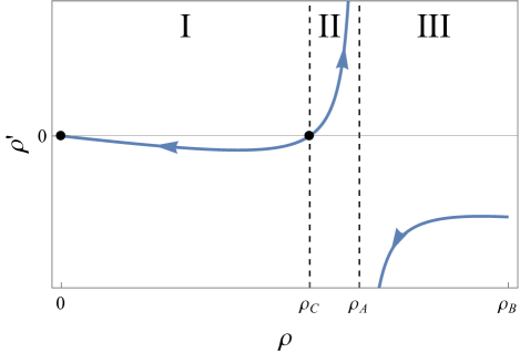
Figure 3: A schematic example of the phase space $(\rho^{\prime},\rho)$ for the case $\rho_{\text{C}}<\rho_{\text{A}}$. The dots represent fixed points, while the arrows represent the flow direction in phase space. The phase space is split into three regions. Region I corresponds to our Universe, while the bouncing solution is confined to region III which is disconnected from our Universe.

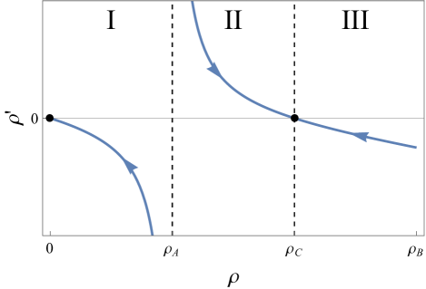
Figure 4: A schematic example of the phase space $(\rho^{\prime},\rho)$ for the case $\rho_{\text{A}}<\rho_{\text{C}}$. The dots represent fixed points, while the arrows represent the flow direction in phase space. The phase space is split into three regions. Region I corresponds to our Universe, while the bouncing solution is confined to region III which is disconnected from our Universe.

IV.2 Case of $\left(T_{\mu\nu}T^{\mu\nu}\right)^{n}$

We can now apply the result of our analysis on generalizations of EMSG that modify the action by adding a term $\left(T_{\mu\nu}T^{\mu\nu}\right)^{n}$ which were studied in Board and Barrow (2017); Akarsu et al. (2018a). The action for these theories (ignoring the cosmological constant) can be written as

$$S=\int d^{4}x\,\sqrt{-g}\,\left(\frac{1}{2\kappa}R-\frac{1}{2}\alpha^{2n-1}\,\left(T_{\mu\nu}T^{\mu\nu}\right)^{n}\right)+S_{\text{M}}\,,$$ (55)

where $\alpha^{-1}$ is the characteristic density scale of this theory, and we will concern ourselves with $n>\frac{1}{2}$ theories, since those are the ones that have relevant effects in the high density regimes.

The effective energy-momentum tensor now becomes

$$T_{\mu\nu}^{\text{eff}}=T_{\mu\nu}-\frac{1}{2}\alpha^{2n-1}\,\left(T_{\sigma\rho}T^{\sigma\rho}\right)^{n}g_{\mu\nu}+n\alpha^{2n-1}\left(T_{\sigma\rho}T^{\sigma\rho}\right)^{n-1}\Theta_{\mu\nu},$$ (56)

where $\Theta_{\mu\nu}$ is defined as before in (5). For a perfect fluid with a barotropic equation of state $p=\omega\rho$, the effective density and pressure become

$$\rho_{\text{eff}} =\rho-\alpha^{2n-1}\rho^{2n}\left(1+3\omega^{2}\right)^{n-1}\left(\left(n-\frac{1}{2}\right)\left(1+3\omega^{2}\right)+4n\omega\right),$$ (57)

$$p_{\text{eff}} =\rho\omega-\frac{1}{2}\alpha^{2n-1}\rho^{2n}\left(1+3\omega^{2}\right)^{n}.$$ (58)

We can easily see that $\rho_{\text{eff}}$ satisfies our assumptions (47) and (49) for $\omega\geq 0$ (which is the case we care about for the moment at least), and it would have a profile similar to the one in Fig. 2. From (57) and (58) we get

$$\rho_{\text{eff}}+p_{\text{eff}}=\rho(1+\omega)\left(1-n(3\omega+1)\alpha^{2n-1}\rho^{2n-1}\left(3\omega^{2}+1\right)^{n-1}\right),$$ (59)

$$\frac{d\rho_{\text{eff}}}{d\rho}=1-2n\alpha^{2n-1}\rho^{2n-1}\left(1+3\omega^{2}\right)^{n-1}\left(\left(n-\frac{1}{2}\right)\left(1+3\omega^{2}\right)+4n\omega\right).$$ (60)

Note that adding a cosmological constant $\Lambda$ would not change the latter expressions. Adding $\Lambda$ is equivalent to the following transformation

$$\rho_{\text{eff}} \rightarrow\rho_{\text{eff}}+\frac{\Lambda}{\kappa},$$

$$p_{\text{eff}} \rightarrow p_{\text{eff}}-\frac{\Lambda}{\kappa},$$ (61)

and $\rho_{\text{eff}}+p_{\text{eff}}$ and $\frac{d\rho_{\text{eff}}}{d\rho}$ are clearly invariant under such a transformation.

By comparing the two expressions in (59) and (60), in order to get the nontrivial zero of $\rho_{\text{eff}}+p_{\text{eff}}$ to coincide with the zero of $\frac{d\rho_{\text{eff}}}{d\rho}$, we see that the only nontrivial value for $n$ that satisfies that condition is (assuming $\omega\geq 0$)

$$n=\frac{3\omega^{2}+3\omega+2}{6\omega^{2}+8\omega+2}.$$ (62)

This value for $n$ leaves the conservation equation unmodified from the one we know in GR (for a single-component fluid with this particular value of $\omega$), namely

$$\rho^{{}^{\prime}}+3\rho\left(1+\omega\right)=0.$$ (63)

For radiation ($\omega=\frac{1}{3}$) that value is $n=\frac{5}{8}$, and hence, $\left(T_{\mu\nu}T^{\mu\nu}\right)^{5/8}$ is the only theory in this class that gives a viable (radiation-dominated) bounce. By solving for the nontrivial zero of $\rho_{\text{eff}}$ in (57) with $n=\frac{5}{8}$ and $\omega=\frac{1}{3}$, the density at the bounce in the $n=\frac{5}{8}$ theory will be equal to $\frac{8}{3\sqrt{3}\alpha}$. Further analysis of this model may be required to ensure that it can reproduce other aspects of standard cosmology; for example, it is important to check the stability of this solution against inhomogeneous perturbations as it may lead to some instabilities similar to those discussed in Peter and Pinto-Neto (2001). In particular, we note that while the $n=5/8$ model avoids any singular behavior in the continuity equation, it is very likely that the effective Euler equation will have singular points due to the nonlinearity of $p_{\text{eff}}$ in $\rho$ and $p$.

It is interesting to note from (62) that for EMSG ($n=1$), we can have a bounce for a dust-only ($\omega=0$) universe.

Finally, we note for completeness that the case $1/2<n<5/8$ is the case corresponding to region I in Fig. 3 which provides a geodesically complete nonsingular solution that can describe our Universe. In these theories the initial singularity is replaced by a de Sitter fixed point (at $t\rightarrow-\infty$), as a result, the Universe is going to interpolate between two fixed points one at a high density and another at a low or vanishing density. It would be interesting to study such theories in future works, particularly with the interpretation of $\alpha^{-1}$as the Planck scale in that case.

V Junction Conditions in EMSG

As we recall, solving the conservation equation (30) and the Friedmann equation (39) led to the following branches of solutions for the scale factor

$$a(t)=a_{\text{min}}\sqrt{1\pm 2H_{\text{max}}t},\,\,\,\,\,\,\,\,\pm t\geq 0,$$ (64)

and the following (independent) branches for $\rho_{r}$:

$$\rho_{r}(a)=\frac{1}{4\alpha}\left(1\pm\sqrt{1-\left(\frac{a_{\text{min}}}{a}\right)^{4}}\right).$$ (65)

In Sec. III, we picked the positive branch for $a$ to get a solution valid for $t>0$, and we picked the negative branch for $\rho_{r}$ to get a solution that corresponds to $\rho_{r}\rightarrow 0$ as $a\rightarrow\infty$. This led to a geometrically nonsingular solution, albeit geodesically incomplete. In this section we will join that solution with the other branch using appropriate junction conditions in order to get a geodesically complete solution, albeit with a curvature singularity at $t=0$. Since EMSG inherits the geometric side of GR, standard junction conditions in GR will be utilized in this section; the reader can be referred to Poisson (2004) for a review.

Using the FRW coordinates, we can define a spacelike hypersurface $\Sigma$ at $t=0$. This hypersurface now splits the spacetime into two regions with $t>0$ and $t<0$ respectively. We can define the following useful notation for the jump in a tensor $A$ across $\Sigma$

$$[A]\equiv A(0^{+})-A(0^{-}).$$ (66)

Here, we have two solutions, one in the region where $t>0$ and the other is in the region where $t<0$; we would like to join them at $\Sigma$. In order to achieve this smoothly, we need two conditions. The first junction condition is

$$[g_{\mu\nu}]=0.$$ (67)

The continuity of the metric here is a very important condition as otherwise the Christoffel symbols would have Dirac deltas, and the curvature tensors then would be ill defined. The second junction condition is

$$[K_{\mu\nu}]=0,$$ (68)

where $K_{\mu\nu}$ is the extrinsic curvature. This condition is necessary for a smooth transition across $\Sigma$; however, a finite jump in $K_{\mu\nu}$ is sufficient for geodesic extension, but it will cause a curvature singularity at $\Sigma$. This singularity has the physical interpretation of having a surface energy momentum tensor at $\Sigma$, which is given by

$$S_{\mu\nu}=\frac{1}{\kappa}\left([K_{\mu\nu}]-[K]h_{\mu\nu}\right),$$ (69)

where $K$ is the trace of the extrinsic curvature and $h_{\mu\nu}$ is the induced metric on $\Sigma$.

We can now start joining the two solutions in (64) at $\Sigma$, we simply get

$$a(t)=a_{\text{min}}\sqrt{1+2H_{\text{max}}|t|}.$$ (70)

We can see that this automatically satisfies the continuity of the metric condition (67). The Hubble rate then becomes

$$H(t)=\frac{H_{\max}}{1+2H_{\text{max}}|t|}\text{sgn}(t).$$ (71)

We can see that the Hubble rate has a finite jump at $t=0$. For the FRW metric with our choice of $\Sigma$, we only need to focus on the spatial components of the extrinsic curvature and the induced metric, which are given by

$$h_{ij}=g_{ij}=a(t)^{2}\delta_{ij},$$ (72)

$$K_{ij}=\frac{1}{2}\partial_{t}h_{ij}=a(t)^{2}H(t)\delta_{ij}.$$ (73)

We can see that the extrinsic curvature picks a finite jump from $H$, which we can calculate as follows

$$[K_{ij}]=2a_{\text{min}}^{2}H_{\text{max}}\delta_{ij},$$ (74)

$$[K]=6H_{\text{max}}.$$ (75)

Since we have a finite jump in the extrinsic curvature, we get a surface energy-momentum tensor contribution (69) as

$$S_{ij}=-\frac{4}{\kappa}a_{\text{min}}^{2}H_{\text{max}}\delta_{ij}.$$ (76)

In GR, this surface energy-momentum tensor would be a contribution to the ordinary energy momentum tensor; however, in the case of EMSG, since the Einstein tensor is sourced by the effective energy momentum tensor instead, (76) is a contribution to the effective energy-momentum tensor, i.e. we have a term like

$$T_{ij}^{\text{eff}}\Bigr{|}_{\Sigma}=\delta(t)S_{ij}.$$ (77)

This is a surface pressure term that is added to the normally occurring $p_{\text{eff}}$ mentioned before. Therefore, the total effective pressure is singular at $\Sigma$. Since the effective pressure is singular at $\Sigma$ while the effective density is finite (which can simply be shown from the Friedmann equation), the singularity at $\Sigma$ is a sudden singularity Barrow (2004). This type of singularities is known to be weak (and hence geodesically extendible) according to Tipler and Krolak’s definitions Tipler (1977); Clarke and Królak (1985) as was shown in Fernández-Jambrina and Lazkoz (2004). Furthermore, the geodesic extendibility here would be the same as in the case considered in Awad (2016) since $a(t)$ in both cases have the same Puiseux expansion up to first order in $t$ (for a more detailed account on the behavior of geodesics according to the Puiseux expansion of the scale factor, see Fernández-Jambrina and Lazkoz (2007)).

Finally, the solution for the density in the region where $t<0$ can be either branch in (65). So the extended solution for all $t$ can either be

$$\rho_{r}(t)=\frac{1}{4\alpha}\left(1-\sqrt{1-\left(\frac{a_{\text{min}}}{a(t)}\right)^{4}}\right),$$ (78)

or

$$\rho_{r}(t)=\frac{1}{4\alpha}\left(1-\text{sgn}(t)\,\sqrt{1-\left(\frac{a_{\text{min}}}{a(t)}\right)^{4}}\right),$$ (79)

where $a(t)$ is given by (70).

It is important to note that the junction conditions in this analysis depended only on two features of the solution; namely, $a(0)=a_{\text{min}}$ and $H(0^{\pm})=\pm H_{\text{max}}$, rather than the full behavior of $a(t)$. These two features are also in the $\left(T_{\mu\nu}T^{\mu\nu}\right)^{n}$ theories with $n>\frac{5}{8}$, and thus they would have the same junction conditions as in this analysis in terms of $a_{\text{min}}$ and $H_{\text{max}}$; the expressions for the latter parameters depend on the choice of $n$ of course.

VI Conclusion

EMSG was first proposed as a theory that cures the initial cosmological singularity, reminiscent of the behavior of theories like loop quantum gravity. We have shown in this work that the regular-bouncing solution one can obtain in such a theory is not viable for our Universe. Instead, the viable solution branch, while having no curvature singularities, is only valid up to a certain point in the past. This branch can be joined with its contracting counterpart using the junction conditions outlined in Sec. V to get a fully extended solution; however, the only way to achieve such an extension is by having a (weak) singularity at the junction. In light of this solution, we see that EMSG can at best provide a singular-bouncing solution, and thus the similarity to theories like loop quantum gravity is only superficial.

The singularity in the extended solution—or the geodesic incompleteness in the non-extended one—suggests that EMSG needs to be corrected at density scales close to $\alpha^{-1}$. This means that EMSG should be interpreted as an effective field theory, valid only at scales away from $\alpha^{-1}$, and one expects new (gravitational) physics to appear at scales at (or beyond) $\alpha^{-1}$. While these new physics do not necessarily have to be quantum, it is more natural to assume that new gravitational physics arise at the Planck scale, and this motivates the interpretation of $\alpha^{-1}$ as the Planck density.

We have also seen that theories that modify GR by effectively modifying the matter Lagrangian must satisfy the stringent condition outlined in Sec. IV in order to have a viable regular-bouncing solution. For the case of $\left(T_{\mu\nu}T^{\mu\nu}\right)^{n}$ generalizations of EMSG, only the $n=5/8$ case satisfies that condition. Aside from bounces, we have shown that theories with $1/2<n<5/8$ can provide a viable nonsingular initially de Sitter solution. It would be interesting to construct arguments similar to those in Sec. IV for more general theories that have a total Lagrangian of the form $f(R,T_{\mu\nu}T^{\mu\nu})$ which would have a more complicated phase space structure.

While only studying the cosmological aspects of EMSG, we have encountered singular points in the matter differential equations due to the nonlinearities introduced in the theory; similar singular behavior can occur in any other physical situation. These singular points can split the phase space, similar to what happened in the cosmology of EMSG, which can cause geodesic incompleteness. Therefore, even for theories that satisfy the condition in Sec. IV, which was obtained for the case of an isotropic universe with perfect fluid content, they may not be valid for all physical scenarios at scales close to their characteristic density scale ($\alpha^{-1}$ in the case of EMSG and its generalizations).

Appendix A Effective Energy-Momentum Tensor

The ordinary energy momentum tensor is defined as

$$T_{\mu\nu}=-\frac{2}{\sqrt{-g}}\frac{\delta\left(\sqrt{-g}L_{m}\right)}{\delta g^{\mu\nu}},$$ (80)

which gives

$$T_{\mu\nu}=L_{m}g_{\mu\nu}-2\frac{\partial L_{m}}{\partial g^{\mu\nu}},$$ (81)

and its variation with respect to the metric is

$$\frac{\delta T_{\sigma\rho}}{\delta g^{\mu\nu}} =-g_{\sigma\mu}g_{\rho\nu}L_{m}+g_{\sigma\rho}\frac{\partial L_{m}}{\partial g^{\mu\nu}}-2\frac{\partial^{2}L_{m}}{\partial g^{\mu\nu}\partial g^{\sigma\rho}}$$ (82)

$$=-g_{\sigma\mu}g_{\rho\nu}L_{m}+g_{\sigma\rho}\left(\frac{1}{2}L_{m}g_{\mu\nu}-\frac{1}{2}T_{\mu\nu}\right)-2\frac{\partial^{2}L_{m}}{\partial g^{\mu\nu}\partial g^{\sigma\rho}}$$ (83)

$$=\left(\frac{1}{2}g_{\sigma\rho}g_{\mu\nu}-g_{\sigma\mu}g_{\rho\nu}\right)L_{m}-\frac{1}{2}T_{\mu\nu}g_{\sigma\rho}-2\frac{\partial^{2}L_{m}}{\partial g^{\mu\nu}\partial g^{\sigma\rho}}.$$ (84)

If we have a theory with the following total action

$$S=\int d^{4}x\,\sqrt{-g}\,\left(\frac{1}{2\kappa}R+L_{m}+F(T_{\sigma\rho}T^{\sigma\rho})\right),$$ (85)

it will be equivalent to having an effective matter Lagrangian as

$$L_{m,\text{eff}}=L_{m}+F(T_{\sigma\rho}T^{\sigma\rho}).$$ (86)

Thus, the effective energy momentum tensor will be

$$T_{\mu\nu}^{\text{eff}} \coloneqq-\frac{2}{\sqrt{-g}}\frac{\delta\left(\sqrt{-g}\,L_{m,\text{eff}}\right)}{\delta g^{\mu\nu}}$$ (87)

$$=T_{\mu\nu}-\frac{2}{\sqrt{-g}}\frac{\delta\left(\sqrt{-g}\,F(T_{\sigma\rho}T^{\sigma\rho})\right)}{\delta g^{\mu\nu}}$$ (88)

$$=T_{\mu\nu}+F(T_{\sigma\rho}T^{\sigma\rho})g_{\mu\nu}-2F_{\boldsymbol{T^{2}}}\Theta_{\mu\nu},$$ (89)

where

$$F_{\boldsymbol{T^{2}}}\equiv\frac{\partial F}{\partial(T_{\sigma\rho}T^{\sigma\rho})},$$ (90)

and

$$\Theta_{\mu\nu}\equiv\frac{\delta\left(T_{\sigma\rho}T^{\sigma\rho}\right)}{\delta g^{\mu\nu}}.$$ (91)

Now what remains is to calculate $\Theta_{\mu\nu}$ as follows

$$\Theta_{\mu\nu} =2T_{\mu\sigma}T_{\,\,\nu}^{\sigma}+2T^{\sigma\rho}\frac{\delta T_{\sigma\rho}}{\delta g^{\mu\nu}}$$ (92)

$$=2T_{\mu\sigma}T_{\,\,\nu}^{\sigma}+2T^{\sigma\rho}\left(\left(\frac{1}{2}g_{\sigma\rho}g_{\mu\nu}-g_{\sigma\mu}g_{\rho\nu}\right)L_{m}-\frac{1}{2}T_{\mu\nu}g_{\sigma\rho}-2\frac{\partial^{2}L_{m}}{\partial g^{\mu\nu}\partial g^{\sigma\rho}}\right)$$ (93)

$$=2T_{\mu\sigma}T_{\,\,\nu}^{\sigma}-2L_{m}\left(T_{\mu\nu}-\frac{1}{2}Tg_{\mu\nu}\right)-TT_{\mu\nu}-4T^{\sigma\rho}\frac{\partial^{2}L_{m}}{\partial g^{\mu\nu}\partial g^{\sigma\rho}},$$ (94)

where we have used the result of (84) in the second line.

Appendix B Matter-Radiation Fluid in EMSG

In EMSG, if we consider a matter-radiation perfect fluid in FRW spacetime, we can get the individual conservation equation for each component by applying the results in (17) on radiation ($\omega=1/3$) and matter ($\omega=0$) respectively, thus we get

$$\left(1-4\alpha\rho_{r}-\frac{7\alpha\rho_{m}}{3}\right)\rho_{r}^{\prime}+4\rho_{r}-8\alpha\rho_{r}^{2}-5\alpha\rho_{m}\rho_{r}=0,$$ (95)

$$\left(1-\alpha\rho_{m}-\frac{7\alpha\rho_{r}}{3}\right)\rho_{m}^{\prime}+3\rho_{m}-3\alpha\rho_{m}^{2}-5\alpha\rho_{r}\rho_{m}=0.$$ (96)

B.0.1 Matter domination

In the case of matter domination, the matter conservation equation (96) becomes

$$\left(1-\alpha\rho_{m}\right)\rho_{m}^{\prime}+3\rho_{m}-3\alpha\rho_{m}^{2} =0$$ (97)

$$\Rightarrow\left(1-\alpha\rho_{m}\right)\left(\rho_{m}^{\prime}+3\rho_{m}\right) =0.$$ (98)

This gives the same behavior as GR, namely $\rho_{m}(a)=\rho_{m0}\,a^{-3}$, where $\rho_{m0}$ is the present matter density and the present scale factor has been set to unity.

The radiation conservation equation (95) becomes

$$\left(1-\frac{7\alpha\rho_{m}}{3}\right)\rho_{r}^{\prime}+4\rho_{r}-5\alpha\rho_{m}\rho_{r}=0,$$ (99)

which gives the solution

$$\rho_{r}(a)=\rho_{r0}\,a^{-4}\left(\frac{1-\frac{7}{3}\alpha\rho_{m0}}{1-\frac{7}{3}\alpha\rho_{m0}a^{-3}}\right)^{13/21}.$$ (100)

In order for $\rho_{r}$ to be real valued, we must have $a\geq\left(\frac{7}{3}\alpha\rho_{m0}\right)^{1/3}$. Therefore we must have a minimum scale in this scenario, which is $a=\left(\frac{7}{3}\alpha\rho_{m0}\right)^{1/3}$. Notice that $\rho_{r}$ diverges as $a\rightarrow\left(\frac{7}{3}\alpha\rho_{m0}\right)^{1/3}$, while $\rho_{m}$ remains finite. Thus, as we get closer to this minimum scale, the radiation part dominates, which contradicts our assumption that we are working in the regime of matter domination. Therefore we can conclude that this solution, which corresponds to a matter dominating era, can only be valid at scales much larger than $\left(\frac{7}{3}\alpha\rho_{m0}\right)^{1/3}$. This gives us a hint that matter dominates away from the early Universe in this theory.

B.0.2 Radiation domination

In the case of radiation domination, the conservation equations for radiation (95) and matter (96) respectively become

$$\left(1-4\alpha\rho_{r}\right)\rho_{r}^{\prime}+4\rho_{r}-8\alpha\rho_{r}^{2}=0,$$ (101)

$$\left(1-\frac{7\alpha\rho_{r}}{3}\right)\rho_{m}^{\prime}+3\rho_{m}-5\alpha\rho_{r}\rho_{m}=0.$$ (102)

These lead to solutions

$$\rho_{m}=\rho_{m0}\left(\frac{3-7\alpha\rho_{r}}{3-7\alpha\rho_{r0}}\right)^{15/14}\left(\frac{1-2\alpha\rho_{r0}}{1-2\alpha\rho_{r}}\right)^{3/4}\left(\frac{\rho_{r}}{\rho_{r0}}\right)^{3/4}$$ (103)

$$\rho_{r}=\frac{1}{4\alpha}\left(1-\sqrt{1-\left(\frac{a_{\text{min}}}{a}\right)^{4}}\right),$$ (104)

where $a_{\text{min}}\equiv\left(8\alpha\rho_{r0}\left(1-2\alpha\rho_{r0}\right)\right)^{1/4}$, and again we have solved using the present values for matter $\rho_{m0}$ and radiation $\rho_{r0}$ while setting the present scale factor $a_{0}$ to unity. We note that the use of present values as conditions in this approximation is still justified since EMSG is expected to coincide with GR at some point in the early Universe; after that point the original equations (95) and (96) will decouple anyway and reduce to their GR counterparts, and hence any condition valid for solving the GR equations after that point is also valid for EMSG, regardless of what component dominates at that condition.

We see from (103) that even at high radiation densities ($\rho_{r}\sim\frac{1}{4\alpha}$), we have

$$\rho_{m}\sim\rho_{m0}\left(\frac{\rho_{r}}{\rho_{r0}}\right)^{3/4},$$ (105)

which is the same behavior of matter as in GR. Therefore the mere requirement that EMSG coincides with GR before the end of the standard radiation dominated era, which is required in order for EMSG to be cosmologically viable, is sufficient for having early-time radiation domination in EMSG. For example, the consistency of EMSG with GR was checked in Akarsu et al. (2018c) where they constrained the parameter $\alpha$ from neutron star observations; their constraint translates to our definition for $\alpha$ (which differs from theirs by a factor of $-1/2$) as

$$0\leq\alpha\lesssim 10^{-38}\,\text{erg}^{-1}\,\text{cm}^{3},$$ (106)

where we only quoted the $\alpha\geq 0$ part of the constraint as it is the one relevant in our case. They then showed that under the upper bound of this constraint, radiation cosmology in EMSG is consistent with standard cosmology up to energy-density scales as high as $10^{-34}\,\text{erg}\,\text{cm}^{-3}$ and time scales as early as $10^{-4}\,\text{s}$. Given that, our result in (103) shows that matter density values would be the same as those in GR (corrections would be extremely small due to the tight constraint on $\alpha$). This automatically means that radiation dominates in the early Universe in EMSG as it does in GR.

References

- Riess et al. (1998) A. G. Riess et al., The Astronomical Journal 116, 1009 (1998).
- Ade et al. (Planck Collaboration) P. A. Ade et al. (Planck Collaboration), Astronomy & Astrophysics 571, A16 (2014).
- Hawking and Penrose (1970) S. W. Hawking and R. Penrose, Proceedings of the Royal Society of London. A. Mathematical and Physical Sciences 314, 529 (1970).
- Clifton et al. (2012) T. Clifton, P. G. Ferreira, A. Padilla, and C. Skordis, Physics Reports 513, 1 (2012).
- Nojiri et al. (2017) S. Nojiri, S. Odintsov, and V. Oikonomou, Physics Reports 692, 1 (2017).
- Ishak (2019) M. Ishak, Living reviews in relativity 22, 1 (2019).
- Novello and Bergliaffa (2008) M. Novello and S. P. Bergliaffa, Physics Reports 463, 127 (2008).
- Battefeld and Peter (2015) D. Battefeld and P. Peter, Physics Reports 571, 1 (2015).
- Roshan and Shojai (2016) M. Roshan and F. Shojai, Phys. Rev. D 94, 044002 (2016).
- Katırcı and Kavuk (2014) N. Katırcı and M. Kavuk, The European Physical Journal Plus 129, 163 (2014).
- Board and Barrow (2017) C. V. R. Board and J. D. Barrow, Phys. Rev. D 96, 123517 (2017).
- Akarsu et al. (2018a) O. Akarsu, N. Katırc ı, and S. Kumar, Phys. Rev. D 97, 024011 (2018a).
- Akarsu et al. (2018b) O. Akarsu, N. Katırc ı, S. Kumar, R. C. Nunes, and M. Sami, Phys. Rev. D 98, 063522 (2018b).
- Akarsu et al. (2019) Ö. Akarsu, J. D. Barrow, C. V. R. Board, N. M. Uzun, and J. A. Vazquez, The European Physical Journal C 79, 846 (2019).
- Akarsu et al. (2018c) O. Akarsu, J. D. Barrow, S. Çıkıntoğlu, K. Y. Ekşi, and N. Katırc ı, Phys. Rev. D 97, 124017 (2018c).
- Faria et al. (2019) M. Faria, C. Martins, F. Chiti, and B. Silva, Astronomy & Astrophysics 625, A127 (2019).
- Bahamonde et al. (2019) S. Bahamonde, M. Marciu, and P. Rudra, Phys. Rev. D 100, 083511 (2019).
- Note (1) was defined as the free parameter in this way in Akarsu et al. (2018c, a).
- Nari and Roshan (2018) N. Nari and M. Roshan, Phys. Rev. D 98, 024031 (2018).
- Schutz (1970) B. F. Schutz, Phys. Rev. D 2, 2762 (1970).
- Brown (1993) J. D. Brown, Classical and Quantum Gravity 10, 1579 (1993).
- Bertolami et al. (2008) O. Bertolami, F. S. N. Lobo, and J. Páramos, Phys. Rev. D 78, 064036 (2008).
- Faraoni (2009) V. Faraoni, Phys. Rev. D 80, 124040 (2009).
- Note (2) When varying the action of a perfect fluid, one gets a set of equations that imply particle number conservation and the conservation of the energy-momentum tensor; see Brown (1993) for a detailed analysis.
- Ashtekar et al. (2006) A. Ashtekar, T. Pawlowski, and P. Singh, Phys. Rev. D 74, 084003 (2006).
- Singh et al. (2006) P. Singh, K. Vandersloot, and G. V. Vereshchagin, Phys. Rev. D 74, 043510 (2006).
- Shtanov and Sahni (2003) Y. Shtanov and V. Sahni, Physics Letters B 557, 1 (2003).
- Note (3) One might object to the use of here, but it is important to note that, since EMSG has to reduce to GR while still being in the radiation dominated era, Eq. (30) reduces to the standard conservation equation for radiation (which is effectively decoupled from other fluid components) where can be used.
- Note (4) Similar analyses can be done using as the main phase space variable, e.g. see Awad (2013).
- Peter and Pinto-Neto (2001) P. Peter and N. Pinto-Neto, Phys. Rev. D 65, 023513 (2001).
- Poisson (2004) E. Poisson, A relativist’s toolkit: the mathematics of black-hole mechanics (Cambridge university press, 2004).
- Barrow (2004) J. D. Barrow, Classical and Quantum Gravity 21, L79 (2004).
- Tipler (1977) F. J. Tipler, Physics Letters A 64, 8 (1977).
- Clarke and Królak (1985) C. Clarke and A. Królak, Journal of Geometry and Physics 2, 127 (1985).
- Fernández-Jambrina and Lazkoz (2004) L. Fernández-Jambrina and R. Lazkoz, Phys. Rev. D 70, 121503 (2004).
- Awad (2016) A. Awad, Phys. Rev. D 93, 084006 (2016).
- Fernández-Jambrina and Lazkoz (2007) L. Fernández-Jambrina and R. Lazkoz, in Journal of Physics: Conference Series, Vol. 66 (IOP Publishing, 2007) p. 012015.
- Martín-García et al. (2004) J. M. Martín-García et al., “xact: Efficient tensor computer algebra for mathematica, http://xact. es/,” (2004).
- Awad (2013) A. Awad, Phys. Rev. D 87, 103001 (2013).