Prompt X-ray emission from Fast Radio Bursts — Upper limits with AstroSat

Abstract

Fast Radio Bursts (FRBs) are short lived ($\sim$ msec), energetic transients (having a peak flux density of $\sim$ Jy) with no known prompt emission in other energy bands. We present results of a search for prompt X-ray emissions from 41 FRBs using the Cadmium Zinc Telluride Imager (CZTI) on AstroSat which continuously monitors $\sim 70\%$ of the sky. Our searches on various timescales in the 20–200 keV range, did not yield any counterparts in this hard X-ray band. We calculate upper limits on hard X-ray flux, in the same energy range and convert them to upper bounds for $\eta$: the ratio X-ray to radio fluence of FRBs. We find $\eta\leq 10^{8-10}$ for hard X-ray emission. Our results will help constrain the theoretical models of FRBs as the models become more quantitative and nearer, brighter FRBs are discovered.

1 Introduction

Fast Radio Bursts (FRBs) are bright ($\sim$ Jy), spatially-unresolved and short ($\sim$ms duration) transients in the radio regime (frequency range of 400 MHz to 8 GHz). These are characterized by their high observed dispersion measures (DMs) — often an order of magnitude higher than the total Galactic electron column density along the line of sight (Yao et al., 2017; Cordes & Lazio, 2002) — indicating that the progenitor is extragalactic. The millisecond duration of the pulse constrains the emission region of the source to $r\lesssim ct_{\mathrm{pulse}}\sim$ 300 km, not considering any relativistic effects in the source frame.

A total of 85 FRB detections have been publicly reported till September 2019 (Petroff et al., 2016a). Of these, 11 FRBs (Spitler et al., 2016a; CHIME/FRB Collaboration et al., 2019a; The CHIME/FRB Collaboration et al., 2019; Kumar et al., 2019) are found to be repeating, but no periodicity or pattern has been found in its repetition (Spitler et al., 2016b; Scholz et al., 2016). Unlike other FRBs, FRB 121102 has been localized, to milli-arcsecond precision, to a dense star forming region of a low-metallicity dwarf galaxy with redshift $z=0.193$ co-located within a projected transverse distance of 40 pc to an unresolved radio source (Chatterjee et al., 2017; Tendulkar et al., 2017; Marcote et al., 2017). This localization and redshift measurement has led to a detailed study of its energetics, host environment (Bassa et al., 2017; Kokubo et al., 2017) and possible links to long Gamma-ray bursts (GRBs) and hydrogen-poor superluminous supernovae (Metzger et al., 2017; Margalit et al., 2018; Margalit & Metzger, 2018).

Until now, no clear physical picture of either the mechanism for an FRB emission or the progenitor has emerged. A wide range of models have been proposed, many of which invoke neutron stars and strong magnetic fields to explain the short duration and high brightness temperatures of FRBs. The astrophysical scenarios hypothesized for the origin of FRBs include Crab-like giant pulses from neutron stars (Cordes & Wasserman, 2016; Katz, 2017), magnetar giant flares (Lyutikov, 2002; Popov & Postnov, 2013; Kulkarni et al., 2014; Pen & Connor, 2015), binary neutron star mergers (Totani, 2013; Paschalidis & Ruiz, 2018), collisions between asteroids and neutron stars (Geng & Huang, 2015), the collapse of a neutron star into a black hole (Falcke & Rezzolla, 2014). There are also non-neutron star models that hypothesize FRBs arising from processes such as Dicke’s superradiance (Houde et al., 2018), axion decay in a strong magnetic field (van Waerbeke & Zhitnitsky, 2018)and compact explosions of macroscopic magnetic dipoles (Thompson, 2017). See Platts et al. (2018); (Popov et al., 2018) for a recent review of FRB observations and models.

The presence or absence of a prompt emission corresponding to FRBs in different wavebands can constrain the emission mechanisms. In models invoking curvature radiation, photons are emitted along the direction of electron motion and the scope for inverse Compton scattering to higher wavebands is small (Kumar et al., 2017; Ghisellini & Locatelli, 2018). If at all, such models predict possible prompt counterparts to FRBs in the THz — optical/infrared regime, but not at X-ray energies. Synchrotron emission models allow for possible inverse Compton upscattering of radio photons to X-ray energies, suggesting prompt X-ray/$\gamma$-ray counterparts for FRBs. Similarly, astrophysical scenarios such as binary neutron star mergers may also lead to the ejection of a GRB jet, which if aligned along our line of sight, will produce a short $\gamma$-ray burst. Radio observations, combined with X-ray, gamma-ray and gravitational wave observations will allow us to constrain the emission mechanisms of FRBs as well as to possibly discover the astrophysical scenarios that lead to them. Totani (2013) states that in particular, if some FRBs are linked to binary neutron star mergers and short GRBs, this may allow us to increase the detection horizon of LIGO and other gravitational wave observatories.

To date high-energy limits on FRB counterparts have been unconstraining due to the relative insensitivity of X-ray/$\gamma$-ray telescopes. Tendulkar et al. (2016) set limits on the fluence ratio in the $\gamma$-ray to radio bands of $F_{\mathrm{\gamma}}/F_{\mathrm{1.4\,GHz}}\lesssim 10^{-7}-10^{-9}\,\mathrm{erg\,cm^{-2}\,Jy^{-1}\,ms^{-1}}$ corresponding to $F_{\mathrm{\gamma}}/F_{\mathrm{1.4\,GHz}}\lesssim 10^{8}-10^{10}$ for a bandwidth of 1 GHz. For most FRBs, these limits are inconsistent with the observational limits for radio emission from the 2007 giant flare of SGR 1806$-$20 (Tendulkar et al., 2016). For FRB 121102, Scholz et al. (2017) set deep limits of $F_{\mathrm{\gamma}}/F_{\mathrm{1.4\,GHz}}<10^{6}-10^{8}$ using simultaneous radio and X-ray observations. We caution that observed values (or limits) of the $\gamma$-ray to radio fluence may significantly differ from intrinsic (source-frame) values due to beaming effects.

There have been a number of efforts at low to intermediate radio frequencies ($\sim$ GHz) searching for prompt counterparts to GRBs, also without significant success. Bannister et al. (2012) searched for short, dispersed radio transients from nine GRBs and detected a few $>6-\sigma$ candidates from two of them with delays of a few hundred seconds compared to the gamma-ray emission. However, the possibility of these being radio frequency interference could not be ruled out. Palaniswamy et al. (2014) searched for radio transients within 140 s of the occurrence of five GRBs but did not detect any significant candidate counterparts. The response time is limited by how fast a large radio dish can slew. In the future, these efforts may be improved by the chances of detecting GRBs in the fields of views of wide field radio telescopes or using software beamforming radio telescopes.

From synchrotron emission, typical expected X-ray to radio ratios are $\sim 10^{4}$ (Lyutikov, 2002) to $10^{6}$ (Lyubarsky, 2014). Pulsars have typical $\gamma$-ray to radio ratios of $10^{4}-10^{8}$. Other theories like Katz (2016), Falcke & Rezzolla (2014) also predict prompt X-ray/$\gamma$-ray emission, though the emission ratios are not well-quantified. These constraints still allow for the possibility of FRBs originating from pulsars, magnetars or other astrophysical scenarios. However, as we discover greater numbers of FRBs, it is important to have a framework to easily search for counterparts and set limits. After we amass a large population of FRBs, especially radio-bright ones, with X-ray non-detections, we can use them to constrain FRB models.

The Cadmium Zinc Telluride Imager (CZTI; Bhalerao et al., 2017a) on board AstroSat (Singh et al., 2014) is a coded aperture mask instrument with a 4$\fdg$6 $\times$ 4$\fdg$6 imaging field of view in the hard X-ray band from 20 keV to 200 keV. The instrument structure is designed to be nearly transparent to photons with energies $\gtrsim 100~{}$keV, making CZTI sensitive to transients from the entire sky, barring $\sim 30\%$ occulted by the Earth. The four identical, independent quadrants of CZTI allow for rejection of spurious signals to a high degree. CZTI has detected over two hundred GRBs. For transients with a clear detection, CZTI data can yield spectra (Rao et al., 2016), polarisation (Vadawale et al., 2015; Chattopadhyay et al., 2017) and localisation (Rao et al., 2016; Bhalerao et al., 2017b).

Here we present a framework for burst searches, the hard X-ray limits on known FRBs and a plan for a near-automated future pipeline.

2 Data Analysis

The standard procedure for CZTI transient searches differs from the usual analysis for steady sources. We outline the transient search method (used, for instance, in Anumarlapudi et al. 2018a, b) in this section. In §3 we expand the sample with searches in archival data.

2.1 Data reduction

CZTI data consists of time-tagged event mode data for individual photons in topocentric frame. AstroSat  is in Low Earth Orbit (LEO) and since the time difference between the ground observatories and AstroSat  is much smaller compared to search window($t_{\mathrm{search}}$), we do not change the frame of reference. The standard CZTI pipeline flags any short duration count rate spikes as noise and removes them from the data. Since this would remove any X-ray photons from FRBs (or Gamma Ray Bursts), we start with unprocessed Level-1 data. The first step is to run cztbunchclean to remove photons created by particle interactions with the satellite. Good Time Intervals (GTIs) are estimated by cztgtigen and data is selected from these GTIs by cztdatasel. Nominally, cztgtigen discards data when the primary target is occulted by Earth. However, as the detector is sensitive to the entire sky, we include this data in our analyses. We then chose initial thresholds (see Table 1) for flagging noisy modules and pixels in cztpixclean to ensure that transients are not suppressed.

Table 1: Parameters used for CZTI search

Parameter	Value
CZT module clean threshold	1000
CZT pixel clean threshold	100
Energy range	20 – 200 keV
Energy bin (qualitative search)	20 keV
Background de-trending	20 s Savitzky Golay filter
Search window ($t_{\mathrm{search}}$)	$-10$ s to $+10$ s
Search timescales ($t_{\mathrm{bin}}$)	0.01 s, 0.1s, 1s

2.2 Qualitative searches

After the data are prepared in this manner, we first undertake a qualitative search for FRB counterparts. We select a $t_{\mathrm{search}}$=20 s window centered on the de-dispersed time of the FRB. We note that the uncertainties in the reported times of the FRBs are much smaller than our search window. For instance, uncertainty in time corresponding to DM error of 0.1 $\mathrm{pc\,cm^{-3}}$ at a frequency of 800 MHz (bottom of the band for UTMOST) will be 0.65 ms, while that of due to AstroSat’s positional error of 1 deg will be 0.78 ms.

Each of the four independent, identical quadrants of CZTI are treated as a separate instrument. We create two dimensional spectrograms (time-energy plots) for the data of each quadrant by binning the data in 20 keV bins in the nominal CZTI energy range of 20–200 keV, and in temporal bins of width $t_{\mathrm{bin}}$ (Figure 1, top). The spectrograms are plotted and visually inspected for excess emission in the $t_{\mathrm{search}}$ window. In this work, we conducted the searches at three timescales: $t_{\mathrm{bin}}$= 10 ms, 100 ms, and 1 s. We do not search at 1 ms timescale: given the effective area of CZTI, the count rate required to ensure at most a single false positive in the $t_{\mathrm{search}}$ window will be an order of magnitude higher than the count rate observed in the succeeding $t_{\mathrm{bin}}$ (10 ms) which means the source has to extremely bright to be able to get detectable at 1 ms timescale. These spectrograms are dominated by the typical “background” spectrum of CZTI, which in our case also includes photons from the on-axis source at the instant of the search. Hence, we also create median-subtracted spectrograms by calculating a median count rate for each energy bin and subtracting it from the instantaneous counts at that energy in each time bin (Figure 1, middle). As a last step, we enhance outliers in each energy bin by dividing the light curve at that energy with its standard deviation calculated over the entire $t_{\mathrm{search}}$ window (Figure 1, bottom). We visually inspect these spectrograms for any signs of enhanced X-ray emission in the $t_{\mathrm{search}}$ window. For all publicly available FRBs where coincident CZTI data were available (Table 2), we did not detect any X-ray candidates.

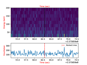
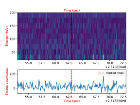
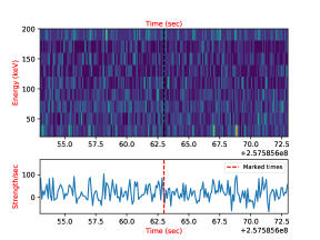
Figure 1: Spectrograms corresponding temporally to search windows centered around arrival time at infinite frequency post dispersive delay correction (TOA) of FRB 180301, marked by a dashed red line. Top Panel: Spectrogram for CZTI quadrant C. Middle Panel: Median subtracted spectrogram. Bottom Panel: Median-subtracted and normalized spectrogram. See §2.2 for more details. All times are UTC, without a barycentric correction.

2.3 Flux limits

Calculation of upper limits for our X-ray non-detections involves three steps. First, we quantify the cut-off count rates above which an FRB would have been detected at high confidence. Second, we calculate the effective area of CZTI in the direction of each FRB. Finally, we assume a spectral model for the X-ray emission and convert the count rate limits into flux upper limits.

The figure of merit we choose for upper limits is the false alarm rate: thus allowing us to put upper limits with a certain confidence. For a candidate to be considered a “detection”, we require coincident detection in all four CZTI quadrants. We select the minimum counts requirement as the point where the probability of accidentally getting those many counts in a quadrant is $F_{\mathrm{quad}}=10\%$. Since the four quadrants are independent, the combined false alarm rate is $F_{\mathrm{quad}}^{4}=10^{-4}$. Hence, we can state that the counts (and flux) from any FRB are lower than our calculated cutoff rates with 99.99% confidence.

If event rates in CZTI were Poisson, we could directly calculate the statistical significance and the false alarm probability of each outlier in the light curve. However, observations have shown that is not true: the data deviate from a Poisson distribution. Hence, we estimate the false alarm rate by actually measuring the behaviour of the count rate in neighbouring data. We take all data from five orbits before and after the instant of the FRB, typically amounting to about 40 ks of data. We process these comparison orbits in the same way as the FRB orbit (§ 2.1). Instead of visual inspection, we now take a more quantitative route. We briefly describe data detrending and cut-off rate estimation here; a more detailed explanation alongside plots is provided in Appendix A.

We calculate light curves for all comparison in the complete energy band (20 – 200 keV), binned at the appropriate $t_{\mathrm{bin}}$. The background count rate is variable on timescales of several minutes based on the position of the satellite around Earth. This slow variation in the background is subtracted off by using a second order Savitzky-Golay filter with a width of 20 seconds. We calculate histograms of count rates from these de-trended light curves, and measure a cutoff rate such that the probability of randomly getting counts above the cutoff rate in a $t_{\mathrm{search}}$ window is $F_{\mathrm{quad}}$. We then create light curves for the $t_{\mathrm{search}}$ window centered on the FRB, and check if the de-trended counts exceed the cutoff rate for that quadrant. As discussed above, a detection would consist of the count rates exceeding the cutoff rates simultaneously in all quadrants. In this study, we repeated this process at all three binning timescales. Based on this criterion, we have X-ray non-detections for all 41 FRBs in our sample.

The sensitivity of the satellite to a burst depends on the location of the burst in the satellite frame of reference. Various satellite elements absorb and scatter incident photons, reducing the number of photons reaching the detector. The sensitivity is highest for on-axis sources, and lowest for bursts that are “seen” through the satellite body. The CZTI team has developed a GEANT4-based mass model of the satellite to calculate the energy- and direction-dependent effective area and response of the satellite. For all FRBs in our sample, we take the coordinates from FRBCAT and convert them into the satellite frame based on the orientation of the satellite at that instant. We then run mass model simulations to calculate the satellite response for each FRB. We note that the effective area and photon energy redistribution (ARF and RMF in X-ray parlance) obtained from the mass model do not change considerably over the uncertainties in the positions of FRBs - hence our inferred upper limits remain reliable.

The last step is the conversion of our cutoff count rates to flux and fluence upper limits for X-ray emission from the FRBs. We start by assuming a simple power law spectrum, $N(E)\propto E^{\Gamma}$, with photon power law index $\Gamma=-1$. The corresponding upper limits on hard X-ray flux are reported in §3. We then estimate $\Gamma_{\mathrm{max}}$, the maximal value of the power law index that is consistent with our assumptions. To do this, we assume a single power law spectrum from radio to hard X-ray energies, and estimate its power law index from our flux limits. This new power law index is used to calculate a new flux limit using our count rate cutoff and the mass model response files. The process is repeated until $\Gamma_{\mathrm{max}}$ converges. Lastly, we use this $\Gamma_{\mathrm{max}}$ value to also calculate limits on the gamma-ray to radio flux ratio that can be compared with past results (§3).

3 Results

For this work, we limit ourselves to the time period from 2015 October 6 (the day CZTI became operational) to 2018 August 31. FRBCAT (Petroff et al., 2016b) lists 64 FRBs in this period — of which 16 were occulted by Earth in the CZTI frame, two were very close to the Earth limb and are ignored, while five occurred while CZTI was non-functional due to a passage of AstroSat through the South Atlantic Anomaly. Table 2 lists the properties of the remaining 41 FRBs that were visible to CZTI. The radio fluences for the Parkes bursts are defined assuming the burst was in the center of the beam, and hence are lower limits. We searched the CZTI data for prompt emission in the 20–200 keV band from the remaining 41 FRBs at three timescales, and did not obtain any detection. Corresponding upper limits on X-ray fluence (erg cm^-2) assuming a simple power-law spectrum with photon index $\Gamma=-1$ are reported in Table 3. The table also reports upper limits on the X-ray to radio fluence ratios ($\eta$) by self-consistently choosing a power-law slope as discussed in §2.3.

4 Discussion

We have set limits on the X-ray to radio fluence ratios that vary between $\sim 10^{7}$ and $\sim 10^{10}$ depending on the intrinsic brightness of the FRB, its location in the radio telescope beam and the location relative to the CZTI field of view. This approaches the range of X-ray to radio fluence ratios expected from theory ($\sim 10^{4}$, Lyutikov 2002 to $10^{6}$, Lyubarsky 2014) and also the range of observed values for pulsars.

DeLaunay et al. (2016) searched the Swift BAT data for any possible $\gamma$-ray emission in the energy range 15-150 KeV and obtained fluence limit of $\mathrm{F_{\gamma}}\lesssim 10^{-6}$ $\mathrm{erg\,cm^{-2}}$ in an interval of 300 sec for a total of 4 FRBs. This corresponds to $\eta$ ($F_{\mathrm{\gamma}}/F_{\mathrm{1.4\,GHz}}$) of $\sim 10^{11}$. We note that the claimed $\gamma$-ray transient detection corresponding to FRB131104 is extremely marginal (illuminating only 2.9$\%$ of the Swift-BAT detector). Further, the search was conducted at much longer timescales ($T_{90}$ = 100 sec) as compared to our study, hence the claimed detection is not at odds with our limits.

However, despite the strong upper limits from non-detections, it is challenging to constrain theories directly based on individual FRB observations because the intrinsic X-ray to radio fluence ratio may be significantly different from the observed ratio due to beaming effects. For instance, some models of binary neutron star mergers suggest that the X-ray/$\gamma$-ray emission would be strongly beamed (as in the case of relativistic jets from GRBs) while the radio emission is relatively isotropic (see for instance, Totani, 2013, and references therein.) In such cases, the lack of observed high-energy emission in an individual case can be dismissed. If the jets are highly relativistic, the emission will be strongly beamed and visible to $<1\%$ of all observers — as happens for gamma ray bursts (Berger, 2014). We need statistical limits on the X-ray to radio fluence ratios on hundreds of FRBs to help us constrain their emission models.

Conversely, if we expect that the radio emission is beamed while the X-ray emission is nearly isotropic (as in the case of a magnetar giant flare), it will be significantly more challenging to verify emission mechanisms. However, in terms of energetics, high-energy emission powered by compact objects with magnetar-like magnetic field strengths cannot be detected at gigaparsec distances unless they are relativistically beamed (Murase et al., 2017).

AstroSat CZTI is one of the most sensitive instruments for detecting short duration high energy transients (see for example Bhalerao et al., 2017b). Our limits on 41 bursts out of 64 that occurred in our search period are consistent with the operational expectations of being sensitive to about half the events, the rest being lost to Earth-occultation and SAA transits. AstroSat continuously records time-tagged photon data which can be used to search for FRB counterparts in ground processing. AstroSat also has the advantage of being sensitive to the entire sky not obstructed by earth: similar to Fermi-LAT but several times larger than the field of view of Swift-BAT. This wide-field hard X-ray sensitivity of CZTI will be very useful in the future as the rate of FRB detections increases with facilities such as CHIME (The CHIME/FRB Collaboration et al., 2018), ASKAP (Johnston et al., 2009), HIRAX (Newburgh et al., 2016) and SKA (Maartens et al., 2015).

Appendix A Estimating Cut off count rate

Here we describe our method for detrending the data and calculating the cut-off rate. To calculate the cut-off count rate, we choose 5 consecutive orbits each, both before and after the event orbit, excluding the orbit of interest. Figure 2 (Top Panel, left) shows the light curve of an entire orbit of one of the quadrants (Quad D) binned at 1 sec. The slow variation in the counts reflects the motion of satellite in its orbit while the data gap is due to satellite’s passage through SAA. We use a second order Savitzky-Golay filter to estimate this background variation and detrend the light curve. The red solid curve in figure 2 (Top Panel, left) shows the estimation of this slow variation using a Savitzky-Golay filter. Figure 2 (Top Panel, right) depicts the 1-s binned light curve after subtracting this slow variation. The average histogram of the count-rates of all 10 neighbouring orbits is used to estimate the cut-off rate, which is quantified by the parameter confidence.

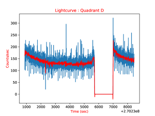
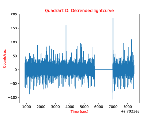
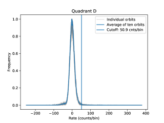
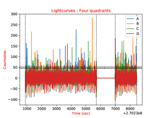
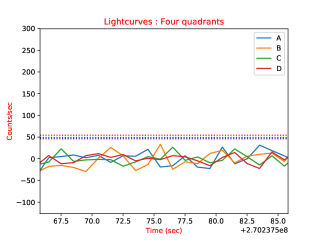
Figure 2: Top Panel: Raw light curve at 1-s binning for one of the four detector quadrants of CZTI. The slowly varying trend due to AstroSat’s orbit and the data gap during SAA passage is visible. Middle Panel:Normalized histogram of the light curve for all the ten individual neighbouring orbits (grey curve) and the resultant average histogram (blue) . Bottom Panel: Left De-trended light curve for the data from the top panel. The vertical dashed lines show data segments that are used. The horizontal dashed lines shows the estimated cut-off count-rate of . Bottom Panel: Right Light curve with quadrant-wise cut-off count rates in the search interval.

Given the time span of the search interval $t_{\mathrm{search}}$, the binning time $t_{\mathrm{bin}}$ and the False Alarm Rate FAR, the chance of detecting a false positive is 1 in ($t_{\mathrm{search}}$/$t_{\mathrm{bin}}$/FAR); hence confidence is 1 - ($t_{\mathrm{search}}$/$t_{\mathrm{bin}}$/FAR). The cut-off rate is chosen based on this required confidence, from the average histogram and is independently estimated for each binning time. It can be noted that the false alarm rate chosen for this analysis is 0.1 per quadrant for a time span of 20s (since the transient is short-lived $\sim$ms) . The four quadrants of CZTI are independent and so the probability of getting a temporally coincident false positive in all the quadrants is $10^{-4}$ in the search interval (20s). The orbital period of AstroSat is $\sim$ 6000s; hence there can be $\sim 30$ false positives per quadrant in an orbit (Figure 2 Bottom Panel, left). However, the requirement of temporal coincidence across quadrants removes such false positives. Figure 2 (Bottom Panel, right) shows the light curve in a 20s window around the arrival time of FRB, with cut off rates for individual quadrants marked. We see no evidence for any temporally coincident prompt emission in all the quadrants above the background level.

Table 2: Observed Parameters of Radio Bursts.

Name	Time	Coordinates (J2000)		Radio Telescope	Central frequency	Bandwidth	$S_{\mathrm{radio}}\tablenotemark{a}$	FWHM	$F_{\mathrm{radio}}\tablenotemark{a}$
	UTC	RA	Dec		MHz	MHz	Jy	ms	Jy-ms
FRB190806	17:07:58.0	00:02:21.38	$-$07:34:54.6	UTMOST	835.0	31.25	3.91	11.96	46.8
FRB190714	05:37:12.901	12:15.9	$-$13:00	ASKAP	1297.0	336.0	4.7	1.7	8.0
FRB190711	01:53:41.100	21:56	$-$80:23	ASKAP	1297.0	336.0	4.11	9.0	28.0
FRB190523	06:05:55.815	13:48:15.6	+72:28:11	DSA$-$10	1405.0	125.0	666.67	0.42	280.0
FRB190322	07:00:12.3	04:46:14.45	$-$66:55:27.8	UTMOST	835.0	31.25	11.85	1.35	16.0
FRB181228	13:48:50.100	06:09:23.64	$-$45:58:02.4	UTMOST	835.0	31.25	19.23	1.24	23.85
FRB181017	10:24:37.400	22:05:54.82	$-$08:50:34.22	UTMOST	835.0	31.25	161	0.32	51.52
FRB180817.J1533+42	01:49:20.202	15:33	+42:12	CHIME/FRB	600.0	400.0	70.27	0.37	26.0
FRB180814.J1554+74	14:20:14.440	15:54	+74:01	CHIME/FRB	600.0	400.0	138.89	0.18	25.0
FRB180812.J0112+80	11:45:32.872	01:12	+80:47	CHIME/FRB	600.0	400.0	14.4	1.25	18.0
FRB180810.J1159+83	22:40:42.493	11:59	+83:07	CHIME/FRB	600.0	400.0	60.71	0.28	17.0
FRB180806.J1515+75	14:13:03.107	15:15	+75:38	CHIME/FRB	600.0	400.0	34.78	0.69	24.0
FRB180801.J2130+72	08:47:14.793	21:30	+72:43	CHIME/FRB	600.0	400.0	54.9	0.51	28.0
FRB180730.J0353+87	03:37:25.937	03:53	+87:12	CHIME/FRB	600.0	400.0	119.05	0.42	50.0
FRB180729.J0558+56	17:28:18.258	05:58	+56:30	CHIME/FRB	600.0	400.0	112.5	0.08	9.0
FRB180727.J1311+26	00:52:04.474	13:11	+26:26	CHIME/FRB	600.0	400.0	17.95	0.78	14.0
FRB180725.J0613+67	17:59:32.813	06:13	+67:04	CHIME/FRB	600.0	400.0	38.71	0.31	12.0
FRB 180528	04:24:00.9	06:38:48.7	$-$49:53:59	UTMOST	835.0	32	15.75	2.0	32
FRB180525	15:19:06.515	14:40	$-$02:12	ASKAP	1297.0	336.0	78.9	3.8	299.82
FRB180430	10:00:35.700	06:51	$-$09:57	ASKAP	1297.0	336.0	147.5	1.2	177.0
FRB180324	09:31:46.706	06:16	$-$34:47	ASKAP	1297.0	336.0	16.5	4.3	70.95
FRB180315	05:05:30.985	19:35	$-$26:50	ASKAP	1297.0	336.0	23.3	2.4	55.92
FRB 180311	04:11:54.800	21:31:33.42	$-$57:44:26.7	Parkes	1352.0	338.381	0.2	12.0	2.4
FRB 180301	07:34:19.760	06:12:43.4	04:33:44.8	Parkes	1352.0	338.381	0.5	3.0	1.5
FRB180212	23:45:04.399	14:21	$-$03:35	ASKAP	1297.0	336.0	53.0	1.81	95.93
FRB180130	04:55:29.993	21:52.2	$-$38:34	ASKAP	1297.0	336.0	23.1	4.1	94.71
FRB180119	12:24:40.747	03:29.3	$-$12:44	ASKAP	1297.0	336.0	40.7	2.7	109.89
FRB180110	07:34:34.959	21:53.0	$-$35:27	ASKAP	1297.0	336.0	128.1	3.2	409.92
FRB171213	14:22:40.467	03:39	$-$10:56	ASKAP	1297.0	336.0	88.6	1.5	132.9
FRB 171209	20:34:23.500	15:50:25	$-$46:10:20	Parkes	1352.0	338.381	0.92	2.5	2.3
FRB171020	10:27:58.598	22:15	$-$19:40	ASKAP	1297.0	336.0	117.6	3.2	376.32
FRB171019	13:26:40.097	22:17.5	$-$08:40	ASKAP	1297.0	336.0	40.5	5.4	218.7
FRB171003	04:07:23.781	12:29.5	$-$14:07	ASKAP	1297.0	336.0	40.5	2.0	81.0
FRB170906	13:06:56.488	21:59.8	$-$19:57	ASKAP	1297.0	336.0	29.6	2.5	74.0
FRB 170827	16:20:18.000	00:49:18.66	$-$65:33:02.3	UTMOST	835.0	32	50.3	0.4	19.87
FRB170707	06:17:34.354	02:59	$-$57:16	ASKAP	1297.0	336.0	14.8	3.5	51.8
FRB170606	10:03:27.000	5:34:0.0	41:45:0.0	Pushchino	111.0	2.5	0.54	3300.0	1782.0
FRB170428	18:02:34.700	21:47	$-$41:51	ASKAP	1320.0	336.0	7.7	4.4	33.88
FRB170416	23:11:12.799	22:13	$-$55:02	ASKAP	1320.0	336.0	19.4	5.0	97.0
FRB 160608	03:53:01.088	07:36:42	$-$40:47:52	UTMOST	843.0	16	4.3	9.0	38.7
FRB 151230	16:15:46.525	09:40:50	$-$03:27:05	Parkes	1352.0	338.381	0.42	4.4	1.9

Table 3: CZTI fluence limits on X-rays from FRBs.

Name	Radio Flux Density	Radio Fluence	tbin	$\Gamma_{max}$	X-ray fluence		$\eta/10^{9}=\frac{F_{X-ray}}{F_{Radio}}/10^{9}$
(Reference to original detection)	Jy	Jy-ms	s		$\mathrm{erg~{}cm^{-2}}$
					$\Gamma=-1$	$\Gamma=\Gamma_{max}$	$\Gamma=-1$	$\Gamma=\Gamma_{max}$
FRB190806	3.91	46.8	0.01	$-$1.19	1.6e$-$07	1.65e$-$07	0.34	0.35
(Gupta et al., 2019a)			0.1	$-$1.25	3.67e$-$07	3.84e$-$07	0.78	0.82
			1.0	$-$1.33	5.69e$-$07	6.03e$-$07	1.21	1.29
FRB190714	4.7	8.0	0.01	$-$1.24	7.38e$-$08	7.47e$-$08	0.92	0.93
(Bhandari et al., 2019)			0.1	$-$1.3	1.67e$-$07	1.69e$-$07	2.08	2.11
			1.0	$-$1.38	2.72e$-$07	2.76e$-$07	3.4	3.45
FRB190711	4.1	28.0	0.01	$-$1.16	4.33e$-$07	4.44e$-$07	1.55	1.59
(Shannon et al., 2019)			0.1	$-$1.22	9.72e$-$07	1.01e$-$06	3.47	3.6
			1.0	$-$1.3	1.55e$-$06	1.64e$-$06	5.55	5.85
FRB190523	666.7	280.0	0.01	$-$1.42	1.53e$-$07	1.61e$-$07	0.05	0.06
(Ravi et al., 2019)			0.1	$-$1.48	3.51e$-$07	3.74e$-$07	0.13	0.13
			1.0	$-$1.56	5.56e$-$07	6.02e$-$07	0.2	0.21
FRB190322	11.8	16.0	0.01	$-$1.23	2.15e$-$07	2.23e$-$07	1.35	1.39
(Gupta et al., 2019b)			0.1	$-$1.29	4.83e$-$07	5.07e$-$07	3.02	3.17
			1.0	$-$1.37	7.53e$-$07	8.02e$-$07	4.7	5.01
FRB181228	19.2	23.8	0.01	$-$1.28	9.74e$-$08	9.6e$-$08	0.41	0.4
Farah et al. (2019)			0.1	$-$1.36	1.38e$-$07	1.36e$-$07	0.58	0.57
			1.0	$-$1.44	2.08e$-$07	2.04e$-$07	0.87	0.85
FRB181017	161.0	51.5	0.01	$-$1.39	6.8e$-$08	6.51e$-$08	0.13	0.13
Farah et al. (2019)			0.1	$-$1.47	9.7e$-$08	9.2e$-$08	0.19	0.18
			1.0	$-$1.55	1.45e$-$07	1.36e$-$07	0.28	0.26
FRB180817.J1533+42	70.3	26.0	0.01	$-$1.3	2.17e$-$07	2.31e$-$07	0.83	0.89
(CHIME/FRB Collaboration et al., 2019b)			0.1	$-$1.36	4.84e$-$07	5.22e$-$07	1.86	2.01
			1.0	$-$1.43	7.57e$-$07	8.33e$-$07	2.91	3.2
FRB180814.J1554+74	138.9	25.0	0.01	$-$1.35	1.18e$-$07	1.21e$-$07	0.47	0.48
(CHIME/FRB Collaboration et al., 2019b)			0.1	$-$1.41	2.71e$-$07	2.78e$-$07	1.08	1.11
			1.0	$-$1.49	4.31e$-$07	4.46e$-$07	1.72	1.78
FRB180812.J0112+80	14.4	18.0	0.01	$-$1.25	1.26e$-$07	1.29e$-$07	0.7	0.72
(CHIME/FRB Collaboration et al., 2019b)			0.1	$-$1.31	2.91e$-$07	3.01e$-$07	1.62	1.67
			1.0	$-$1.39	4.41e$-$07	4.62e$-$07	2.45	2.57
FRB180810.J1159+83	60.7	17.0	0.01	$-$1.2	1.85e$-$06	2e$-$06	10.89	11.74
(CHIME/FRB Collaboration et al., 2019b)			0.1	$-$1.26	4.29e$-$06	4.74e$-$06	25.24	27.89
			1.0	$-$1.33	6.91e$-$06	7.89e$-$06	40.66	46.39
FRB180806.J1515+75	34.8	24.0	0.01	$-$1.27	2.22e$-$07	2.30e$-$07	0.93	0.96
(CHIME/FRB Collaboration et al., 2019b)			0.1	$-$1.33	5.1e$-$07	5.34e$-$07	2.13	2.23
			1.0	$-$1.4	8.1e$-$07	8.6e$-$07	3.37	3.58
FRB180801.J2130+72	54.9	28.0	0.01	$-$1.29	2.01e$-$07	2.10e$-$07	0.72	0.75
(CHIME/FRB Collaboration et al., 2019b)			0.1	$-$1.35	4.58e$-$07	4.85e$-$07	1.64	1.73
			1.0	$-$1.43	7.21e$-$07	7.75e$-$07	2.57	2.77
FRB180730.J0353+87	119.0	50.0	0.01	$-$1.31	2.80e$-$07	2.875e$-$07	0.56	0.58
(CHIME/FRB Collaboration et al., 2019b)			0.1	$-$1.37	6.42e$-$07	6.64e$-$07	1.28	1.33
			1.0	$-$1.44	9.96e$-$07	1.04e$-$06	1.99	2.08
FRB180729.J0558+56	112.5	9.0	0.01	$-$1.3	3.34e$-$07	3.52e$-$07	3.71	3.91
(CHIME/FRB Collaboration et al., 2019b)			0.1	$-$1.36	7.47e$-$07	7.98e$-$07	8.3	8.86
			1.0	$-$1.43	1.22e$-$06	1.33e$-$06	13.59	14.76
FRB180727.J1311+26	18.0	14.0	0.01	$-$1.21	4.93e$-$07	5.08e$-$07	3.52	3.63
(CHIME/FRB Collaboration et al., 2019b)			0.1	$-$1.27	1.09e$-$06	1.14e$-$06	7.82	8.15
			1.0	$-$1.34	1.72e$-$06	1.82e$-$06	12.32	13.02
FRB180725.J0613+67	38.7	12.0	0.01	$-$1.25	3.73e$-$07	3.96e$-$07	3.11	3.3
(CHIME/FRB Collaboration et al., 2019b)			0.1	$-$1.31	8.73e$-$07	9.43e$-$07	7.28	7.86
			1.0	$-$1.38	1.39e$-$06	1.53e$-$06	11.57	12.77
FRB180528	15.8	32.0	0.01	$-$1.24	1.21e$-$06	1.31e$-$06	3.77	4.1
Farah et al. (2019)			0.1	$-$1.3	2.752e$-$06	3.07e$-$06	8.6	9.6
			1.0	$-$1.38	4.32e$-$06	4.97e$-$06	13.49	15.55
FRB180525	78.9	299.8	0.01	$-$1.35	8.14e$-$08	8.23e$-$08	0.03	0.03
(Macquart et al., 2019)			0.1	$-$1.42	1.85e$-$07	1.87e$-$07	0.06	0.06
			1.0	$-$1.5	2.94e$-$07	2.99e$-$07	0.1	0.1
FRB180430	147.5	177.0	0.01	$-$1.32	2.85e$-$07	3.065e$-$07	0.16	0.17
(Qiu et al., 2019)			0.1	$-$1.39	6.43e$-$07	7.03e$-$07	0.36	0.4
			1.0	$-$1.46	1.04e$-$06	1.16e$-$06	0.59	0.65
FRB180324	16.5	71.0	0.01	$-$1.26	1.59e$-$07	1.64e$-$07	0.22	0.23
(Macquart et al., 2019)			0.1	$-$1.32	3.57e$-$07	3.72e$-$07	0.5	0.52
			1.0	$-$1.4	5.46e$-$07	5.76e$-$07	0.77	0.81
FRB180315	23.3	55.9	0.01	$-$1.2	9.84e$-$07	1.03e$-$06	1.76	1.84
(Macquart et al., 2019)			0.1	$-$1.26	2.25e$-$06	2.39e$-$06	4.03	4.28
			1.0	$-$1.34	3.48e$-$06	3.77e$-$06	6.22	6.74
FRB180311	0.2	2.4	0.01	$-$1.02	5.435e$-$07	5.46e$-$07	22.64	22.76
(Osłowski et al., 2019)			0.1	$-$1.08	1.20e$-$06	1.23e$-$06	50.17	51.25
			1.0	$-$1.16	2.01e$-$06	2.095e$-$06	83.68	87.28
FRB180301	0.5	1.5	0.01	$-$1.11	1.72e$-$07	1.74e$-$07	11.46	11.63
(Price et al., 2018)			0.1	$-$1.17	3.86e$-$07	3.95e$-$07	25.71	26.33
			1.0	$-$1.25	6.21e$-$07	6.44e$-$07	41.39	42.96
FRB180212	53.0	95.9	0.01	$-$1.34	8.71e$-$08	8.75e$-$08	0.09	0.09
(Shannon et al., 2018)			0.1	$-$1.4	2.03e$-$07	2.05e$-$07	0.21	0.21
			1.0	$-$1.47	3.44e$-$07	3.48e$-$07	0.36	0.36
FRB180130	23.1	94.7	0.01	$-$1.18	1.25e$-$06	1.35e$-$06	1.32	1.42
(Shannon et al., 2018)			0.1	$-$1.25	2.86e$-$06	3.14e$-$06	3.01	3.32
			1.0	$-$1.32	4.79e$-$06	5.45e$-$06	5.06	5.76
FRB180119	40.7	109.9	0.01	$-$1.31	1.07e$-$07	1.10e$-$07	0.1	0.1
(Shannon et al., 2018)			0.1	$-$1.38	2.36e$-$07	2.44e$-$07	0.21	0.22
			1.0	$-$1.46	3.85e$-$07	4.02e$-$07	0.35	0.37
FRB180110	128.1	409.9	0.01	$-$1.33	2.21e$-$07	2.36e$-$07	0.05	0.06
(Shannon et al., 2018)			0.1	$-$1.39	5.1e$-$07	5.54e$-$07	0.12	0.14
			1.0	$-$1.47	7.88e$-$07	8.74e$-$07	0.19	0.21
FRB171213	88.6	132.9	0.01	$-$1.33	1.68e$-$07	1.77e$-$07	0.13	0.13
(Shannon et al., 2018)			0.1	$-$1.39	3.82e$-$07	4.08e$-$07	0.29	0.31
			1.0	$-$1.47	6.14e$-$07	6.67e$-$07	0.46	0.5
FRB171209	0.92	2.3	0.01	$-$1.28	1.9e$-$07	1.79e$-$07	8.26	7.78
(Osłowski et al., 2019)			0.1	$-$1.3	2.8e$-$07	2.98e$-$07	12.17	12.96
			1.0	$-$1.32	4.5e-07	4.77e-07	19.57	20.74
FRB171020	117.6	376.3	0.01	$-$1.37	9e$-$08	9.05e$-$08	0.02	0.02
(Shannon et al., 2018)			0.1	$-$1.43	1.99e$-$07	2.01e$-$07	0.05	0.05
			1.0	$-$1.51	3.36e$-$07	3.4e$-$07	0.09	0.09
FRB171019	40.5	218.7	0.01	$-$1.34	5.93e$-$08	5.92e$-$08	0.03	0.03
(Shannon et al., 2018)			0.1	$-$1.4	1.3e$-$07	1.3e$-$07	0.06	0.06
			1.0	$-$1.48	2.22e$-$07	2.23e$-$07	0.1	0.1
FRB171003	40.5	81.0	0.01	$-$1.25	4.42e$-$07	4.50e$-$07	0.55	0.56
(Shannon et al., 2018)			0.1	$-$1.32	1.01e$-$06	1.03e$-$06	1.24	1.27
			1.0	$-$1.39	1.72e$-$06	1.78e$-$06	2.13	2.2
FRB170906	29.6	74.0	0.01	$-$1.28	1.62e$-$07	1.68e$-$07	0.22	0.23
(Shannon et al., 2018)			0.1	$-$1.34	3.68e$-$07	3.86e$-$07	0.5	0.52
			1.0	$-$1.42	6.01e$-$07	6.39e$-$07	0.81	0.86
FRB170827	50.3	19.9	0.01	$-$1.32	1.10e$-$07	1.15e$-$07	0.55	0.58
(Farah et al., 2017)			0.1	$-$1.38	2.44e$-$07	2.58e$-$07	1.23	1.3
			1.0	$-$1.45	3.97e$-$07	4.25e$-$07	2.0	2.14
FRB170707	14.8	51.8	0.01	$-$1.26	1.42e$-$07	1.46e$-$07	0.27	0.28
(Shannon et al., 2018)			0.1	$-$1.32	3.13e$-$07	3.25e$-$07	0.6	0.63
			1.0	$-$1.4	5.05e$-$07	5.32e$-$07	0.98	1.03
FRB170606	0.5	1782.0	0.01	$-$1.02	1.38e$-$06	1.39e$-$06	0.08	0.08
Rodin & Fedorova (2018)			0.1	$-$1.08	3.13e$-$06	3.21e$-$06	0.18	0.18
			1.0	$-$1.15	4.75e$-$06	5.01e$-$06	0.27	0.28
FRB170428	7.7	33.9	0.01	$-$1.2	2.715e$-$07	2.80e$-$07	0.8	0.83
(Shannon et al., 2018)			0.1	$-$1.27	6.13e$-$07	6.38e$-$07	1.81	1.88
			1.0	$-$1.34	9.71e$-$07	1.03e$-$06	2.86	3.03
FRB170416	19.4	97.0	0.01	$-$1.22	4.525e$-$07	4.79e$-$07	0.47	0.49
(Shannon et al., 2018)			0.1	$-$1.28	1.0e$-$06	1.085e$-$06	1.04	1.12
			1.0	$-$1.36	1.56e$-$06	1.73e$-$06	1.61	1.78
FRB160608	4.3	38.7	0.01	$-$1.11	1.88e$-$06	1.29e$-$06	4.85	3.34
Caleb et al. (2018)			0.1	$-$1.17	4.25e$-$06	3e$-$06	10.99	7.75
			1.0	$-$1.25	6.69e$-$06	4.87e$-$06	17.29	12.57
FRB151230	0.4	1.9	0.01	$-$1.1	1.78e$-$07	1.80e$-$07	9.36	9.49
(Bhandari et al., 2018)			0.1	$-$1.16	4e$-$07	4.09e$-$07	21.05	21.54
			1.0	$-$1.24	6.76e$-$07	7e$-$07	35.57	36.87

References

- Anumarlapudi et al. (2018a) Anumarlapudi, A., Aarthy, E., Arvind, B., et al. 2018a, The Astronomer’s Telegram, 11417, 1
- Anumarlapudi et al. (2018b) —. 2018b, The Astronomer’s Telegram, 11413, 1
- Astropy Collaboration et al. (2013) Astropy Collaboration, Robitaille, T. P., Tollerud, E. J., et al. 2013, A&A, 558, A33
- Bannister et al. (2012) Bannister, K. W., Murphy, T., Gaensler, B. M., & Reynolds, J. E. 2012, ApJ, 757, 38
- Bassa et al. (2017) Bassa, C. G., Tendulkar, S. P., Adams, E. A. K., et al. 2017, ApJ, 843, L8
- Berger (2014) Berger, E. 2014, Annual Review of Astronomy and Astrophysics, 52, 43. http://adsabs.harvard.edu/abs/2014ARA{%}2526A..52...43B
- Bhalerao et al. (2017a) Bhalerao, V., Bhattacharya, D., Vibhute, A., et al. 2017a, Journal of Astrophysics and Astronomy, 38, 31
- Bhalerao et al. (2017b) Bhalerao, V., Kasliwal, M. M., Bhattacharya, D., et al. 2017b, ApJ, 845, 152
- Bhandari et al. (2019) Bhandari, S., Kumar, P., Shannon, R. M., & Macquart, J. P. 2019, The Astronomer’s Telegram, 12940, 1
- Bhandari et al. (2018) Bhandari, S., Keane, E. F., Barr, E. D., et al. 2018, MNRAS, 475, 1427
- Blackburn (1995) Blackburn, J. K. 1995, in Astronomical Society of the Pacific Conference Series, Vol. 77, Astronomical Data Analysis Software and Systems IV, ed. R. A. Shaw, H. E. Payne, & J. J. E. Hayes, 367
- Caleb et al. (2018) Caleb, M., Flynn, C., Bailes, M., et al. 2018, in IAU Symposium, Vol. 337, Pulsar Astrophysics the Next Fifty Years, ed. P. Weltevrede, B. B. P. Perera, L. L. Preston, & S. Sanidas, 322–323
- Chatterjee et al. (2017) Chatterjee, S., Law, C. J., Wharton, R. S., et al. 2017, Nature, 541, 58
- Chattopadhyay et al. (2017) Chattopadhyay, T., Vadawale, S. V., Aarthy, E., et al. 2017, ArXiv e-prints, arXiv:1707.06595