Axion-photon-dark photon oscillation and its implication for 21 cm observation

Abstract

We examine the resonant conversion of axion-like particle (ALP) or dark photon to the electromagnetic photon in the early Universe, which takes place due to the ALP-photon-dark photon oscillations in background dark photon gauge fields. It is noted that the corresponding conversion probability can have an unusual spectral feature which allows strong conversion at low frequency domain, but has negligible conversion at high frequencies above certain critical frequency which is determined by the ALP coupling to dark photon and the strength of background dark photon gauge field. We apply this scheme to heat up the 21 cm photons without affecting the Cosmic Microwave Background, which can explain the tentative absorption signal of 21 cm photons detected recently by the EDGES experiment.

1 Introduction

In spite of the great success of the Standard Model (SM) of particle physics, there are many reasons to contemplate new physics beyond the Standard Model (BSM). Although it needs to be confirmed later, the recent EDGES data Bowman:2018yin of the Rayleigh-Jeans tail of the Cosmic Microwave Background (CMB) may provide another indication of BSM physics as it can be interpreted as an anomalously strong absorption signal of the 21 cm photons. There can be two approaches to explain the EDGES anomaly, either cool down baryons to lower the spin temperature Barkana:2018lgd or heat up the 21 cm photons. For the latter approach, an efficient way is to utilize resonant conversion of dark radiations (DR) to 21 cm photons in the early Universe, which occurs at the redshift in the range $20<z<1700$ Pospelov:2018kdh ; Moroi:2018vci . Such scenario involves an ultra-light DR with a mass satisfying the resonance condition $m_{\rm DR}=m_{\gamma}(z)={\cal O}(10^{-14}-10^{-9})\,{\rm eV}$ for $20<z<1700$, where $m_{\gamma}(z)$ is the effective photon mass in the early Universe, as well as an appropriate coupling of DR to induce the necessary conversion to photons. There are two appealing candidates for such DR, an axion-like particle (ALP) and a dark photon Pospelov:2018kdh ; Moroi:2018vci .

Nonetheless, the scheme to heat up 21 cm photons is facing with many observational constraints and also theoretical concerns on its naturalness. One of the major constraints comes from the distortion of CMB due to the conversion of CMB to DR Mirizzi:2009iz ; Mirizzi:2009nq . Yet its significance severely depends on the spectral feature of the conversion probability, which is often determined by the scaling property of the underlying coupling. For instance, for the conversion of dark photons to 21 cm photons Pospelov:2018kdh , the underlying coupling is the mass-dimension $d=4$ kinetic mixing

$$\frac{1}{2}\varepsilon F_{\mu\nu}X^{\mu\nu},$$ (1)

where $F^{\mu\nu}$ and $X^{\mu\nu}$ are the field strengths of the electromagnetic photon $\gamma$ and the dark photon $\gamma^{\prime}$, respectively. One then finds the resonant conversion probability $P_{\gamma\leftrightarrow\gamma^{\prime}}\propto\varepsilon^{2}/\omega$ Pospelov:2018kdh ; Mirizzi:2009iz , where the dependence on the photon frequency $\omega$ originates from relativistic kinematics. As $\omega_{\rm CMB}\sim 10^{3}\,\omega_{21}$, the conversion at the CMB frequency $\omega_{\rm CMB}$ is suppressed relative to the conversion at the 21 cm frequency $\omega_{21}$. This makes it possible that sizable parameter region can avoid a dangerous distortion of CMB. However this scenario needs a symmetry breaking sector to generate a tiny dark photon mass $m_{\gamma^{\prime}}={\cal O}(10^{-14}-10^{-9})\,{\rm eV}$, which may cause a severe naturalness problem or require an uncomfortably low cutoff scale of the model as was discussed recently in Reece:2018zvv . It requires also a small kinetic mixing $\varepsilon<10^{-5}$ Pospelov:2018kdh , which may cause another fine tuning problem in the UV completion of the model.

For the scenario utilizing the resonant conversion of ALP to photons in background magnetic field Moroi:2018vci , the required small ALP mass $m_{a}={\cal O}(10^{-14}-10^{-9})\,{\rm eV}$ can be achieved by a tiny non-perturbative breaking of the ALP shift symmetry $U(1)_{a}:a\rightarrow a+{\rm constant}$ without causing a naturalness problem. The main difficulty of this scenario originates from the observational constraints on the underlying ALP coupling

$$\frac{1}{4}g_{a\gamma\gamma}aF^{\mu\nu}\tilde{F}_{\mu\nu},$$ (2)

where $\tilde{F}_{\mu\nu}=\frac{1}{2}\epsilon_{\mu\nu\rho\sigma}F^{\rho\sigma}$ is the dual electromagnetic field strength. As this coupling has a mass-dimension $d=5$, the conversion is more efficient at higher frequency as $P_{\gamma\leftrightarrow a}\propto g_{a\gamma\gamma}^{2}\omega$. Then the conversion at $\omega_{\rm CMB}$ is much stronger than the conversion at $\omega_{21}$, making the constraint from the CMB distortion quite severe. There exist also other constraints to be taken, for instance an upper bound on $g_{a\gamma\gamma}$ from the absence of $\gamma$-ray burst associated with SN1987A Payez:2014xsa , and also an upper bound on the primordial background magnetic field, $B_{0}\lesssim 0.1$ nG, to avoid an overheating of baryons which would wash away the EDGES signal Minoda:2018gxj . As is presented in Appendix C, taking these constraints together, only a tiny parameter region of $(m_{a},g_{a\gamma\gamma})$ can provide a viable explanation for the EDGES anomaly even when one assumes the most optimistic spectrum of ALP dark radiation and also a primordial background magnetic field $B_{0}\sim 0.1$ nG which is close to its upper bound.

In this paper, we wish to explore an alternative scheme to explain the EDGES anomaly. Our scheme involves both an ALP with $m_{a}\lesssim 10^{-9}\,{\rm eV}$ and a massless dark photon. It is utilizing again the resonant conversion of ALP or dark photon to 21 cm photons, but based on the photon-ALP-dark photon oscillation in background dark photon gauge field, which is induced by the ALP couplings

$$\frac{1}{2}g_{a\gamma\gamma^{\prime}}aF_{\mu\nu}\tilde{X}^{\mu\nu}+\frac{1}{4}g_{a\gamma^{\prime}\gamma^{\prime}}aX_{\mu\nu}\tilde{X}^{\mu\nu}.$$ (3)

As the dark photon $X_{\mu}$ is exactly massless, we don’t need an additional sector to break the dark photon $U(1)_{X}$ gauge symmetry. A key ingredient of our scheme is a nonzero primordial background dark photon gauge field strength $\langle X_{\mu\nu}\rangle$, which can be easily generated in the early Universe as was demonstrated in Choi:2018dqr . In the presence of $\langle X_{\mu\nu}\rangle\neq 0$, the ALP coupling $g_{a\gamma\gamma^{\prime}}$ induces a mixing between $\gamma$ and ALP, while $g_{a\gamma^{\prime}\gamma^{\prime}}$ induces a mixing between another pair, $\gamma^{\prime}$ and ALP. As a consequence, the two ALP couplings in (3) result in oscillations among the three different particle states $\gamma$, $\gamma^{\prime}$ and ALP in background $\langle X_{\mu\nu}\rangle$.

As for the spectral dependence of the conversion probability $P_{\gamma\leftrightarrow a,\gamma^{\prime}}$ in our scheme, it reveals an unusually interesting feature. The conversion probability can be large enough, even close to unity, over a certain frequency range below $\omega_{c}$, but sharply drops to a negligibly small value at higher frequencies above $\omega_{c}$, where the critical frequency $\omega_{c}\propto 1/g_{a\gamma^{\prime}\gamma^{\prime}}\langle X_{\mu\nu}\rangle$ is determined by the ALP coupling $g_{a\gamma^{\prime}\gamma^{\prime}}$ and the strength of the background dark photon gauge field $\langle X_{\mu\nu}\rangle$ (see Fig. 3). Then the EDGES anomaly can be explained, while avoiding a dangerous CMB distortion, for the model parameters yielding $\omega_{21}<\omega_{c}<\omega_{\rm CMB}$, which can be achieved when

$$4.6\times 10^{-8}\,{\rm GeV}^{-1}\mu{\rm G}\,<\,g_{a\gamma^{\prime}\gamma^{\prime}}\langle X_{\mu\nu}\rangle\,<\,3.7\times 10^{-5}\,{\rm GeV}^{-1}\mu{\rm G}.$$ (4)

As we need $\langle X_{\mu\nu}\rangle\lesssim 1\,\mu{\rm G}$ to avoid a too large dark radiation energy density, the above condition implies

$$g_{a\gamma^{\prime}\gamma^{\prime}}\,\gtrsim\,4\times 10^{-8}\,{\rm GeV}^{-1}.$$ (5)

Yet the other ALP couplings $g_{a\gamma\gamma^{\prime}}$ and $g_{a\gamma\gamma}$ can be small enough to be phenomenologically safe without causing a fine tuning problem. For instance, $g_{a\gamma\gamma^{\prime}}$ and $g_{a\gamma\gamma}$ can originate from $g_{a\gamma^{\prime}\gamma^{\prime}}$ through a loop-induced kinetic mixing $\varepsilon={\cal O}(10^{-3}-10^{-2})$ between $\gamma$ and $\gamma^{\prime}$, which would result in $g_{a\gamma\gamma}\sim\varepsilon g_{a\gamma\gamma^{\prime}}\sim\varepsilon^{2}g_{a\gamma^{\prime}\gamma^{\prime}}$. Alternatively, one may utilize the clockwork mechanism Choi:2014rja ; Choi:2015fiu ; Kaplan:2015fuy to achieve a hierarchical pattern of ALP couplings, which can generate even an exponentially small $g_{a\gamma\gamma^{\prime}}/g_{a\gamma^{\prime}\gamma^{\prime}}$ Higaki:2015jag ; Farina:2016tgd ; Agrawal:2017cmd . Such mechanisms then allow the ALP couplings to satisfy the astrophysical constraints $g_{a\gamma\gamma^{\prime}}<5\times 10^{-10}\,{\rm GeV}^{-1}$ Choi:2018mvk and $g_{a\gamma\gamma}<5\times 10^{-12}\,{\rm GeV}^{-1}$ Payez:2014xsa even when $g_{a\gamma^{\prime}\gamma^{\prime}}$ is as large as (5).

An appealing feature of our scheme is that $P_{\gamma\leftrightarrow a,\gamma^{\prime}}$ at $\omega_{21}$ can be close to unity over a wide range of model parameters satisfying the observational constraints. Therefore our scheme can explain the EDGES anomaly even with a small amount of dark radiations in the 21 cm frequency range. Another interesting feature is that the EDGES anomaly can be explained even when the ALP mass $m_{a}\ll m_{\gamma}(z\simeq 20)\sim 10^{-14}$ eV. Even in such case of ultra-light $m_{a}$, resonance conversion of DR to 21 cm photons can take place during the period $20<z<1700$ through an effective DR mass which is determined mostly by $g_{a\gamma^{\prime}\gamma^{\prime}}\langle X_{\mu\nu}\rangle$.

The organization of this paper is as follows. In the next section, we discuss the resonant conversion between the photon and dark radiation composed of ALPs and dark photons, which can take place in the early Universe involving a non-zero background dark photon gauge field. In Sec. 3, we apply this scheme to the EDGES anomaly and identify the parameter region which can explain the EDGES signal while satisfying the observational constraints. We then conclude in Sec. 4. To supplement our discussion, we provide in Appendix A a brief summary of the key features of the resonant conversion between the photon and a generic dark radiation in the early Universe; discuss in Appendix B an explicit scheme to generate a primordial background dark photon gauge field based on the mechanism of Choi:2018dqr ; and finally update in Appendix C the observational constraints on the ALP scenario of Moroi:2018vci .

2 Resonant conversion in ALP-photon-dark photon oscillation scenario

In this section, we discuss the resonant conversion between $\gamma$ and the dark sector particles composed of ALP and dark photon, which can take place in the early Universe under nonzero background dark photon gauge field. In models with an ALP and a dark photon, there can be ALP couplings of the form

$$\frac{1}{4}g_{a\gamma\gamma}aF_{\mu\nu}\tilde{F}^{\mu\nu}+\frac{1}{2}g_{a\gamma\gamma^{\prime}}aF_{\mu\nu}\tilde{X}^{\mu\nu}+\frac{1}{4}g_{a\gamma^{\prime}\gamma^{\prime}}aX_{\mu\nu}\tilde{X}^{\mu\nu},$$ (6)

where $F_{\mu\nu}=\partial_{\mu}A_{\nu}-\partial_{\nu}A_{\mu}$ is the field strength of the ordinary electromagnetic gauge field $A_{\mu}$, $\tilde{F}^{\mu\nu}=\frac{1}{2}\epsilon^{\mu\nu\rho\sigma}F_{\rho\sigma}$ is its dual field strength, and $X_{\mu\nu}=\partial_{\mu}X_{\nu}-\partial_{\nu}X_{\mu}$ is the field strength of the $U(1)_{X}$ dark photon gauge field $X_{\mu}$. We assume that the dark photon is massless in order to have a long-range cosmic background dark photon gauge field, which is one of the key ingredients of our scheme. This also allows us to avoid $U(1)_{X}$ breaking sector which may cause a naturalness problem. Note that for massless $X_{\mu}$, the kinetic mixing between $A_{\mu}$ and $X_{\mu}$ can be rotated away by an appropriate field redefinition of $X_{\mu}$ and $A_{\mu}$, and the above ALP couplings are defined in such field basis.

In the presence of background dark photon gauge field

$$\langle X_{\mu\nu}\rangle=(\vec{E}_{X},\vec{B}_{X}),$$ (7)

the above ALP couplings affect the evolution of the involved particles. We find the corresponding evolution equation in relativistic limit is given by

$$\left[i\frac{d}{dt}-\frac{1}{2\omega}\mathcal{M}^{2}\right]\left(\begin{array}[]{c}A_{\parallel}\\ X_{\parallel}\\ a\end{array}\right)=0\,,$$ (11)

where $A_{\parallel}$ and $X_{\parallel}$ denote the polarization states of $A_{\mu}$ and $X_{\mu}$ parallel to the background dark photon gauge field combination

$$\vec{\cal B}_{X}=\vec{B}_{X}-\hat{k}(\hat{k}\cdot\vec{B}_{X})-\hat{k}\times\vec{E}_{X},$$ (12)

and the effective mass-square matrix is

$$\mathcal{M}^{2}=\left[\begin{array}[]{ccc}m_{\gamma}^{2}&0&m_{\gamma a}^{2}\\ 0&0&m_{\gamma^{\prime}a}^{2}\\ m_{\gamma a}^{2}&m_{\gamma^{\prime}a}^{2}&m_{a}^{2}\end{array}\right]$$ (16)

where

$$m_{\gamma a}^{2}=g_{a\gamma\gamma^{\prime}}{\cal B}_{X}\omega,\quad m_{\gamma^{\prime}a}^{2}=g_{a\gamma^{\prime}\gamma^{\prime}}{\cal B}_{X}\omega\quad\left({\cal B}_{X}=|\vec{\cal B}_{X}|\right).$$ (17)

Here $(\omega,\vec{k})$ denote the energy and momentum of the involved particles, $\hat{k}=\vec{k}/|\vec{k}|$, and we include also the effective photon mass $m_{\gamma}$ induced by the background thermal plasma in the early Universe.

In order to derive the resonant conversion rate, we need information on the effective photon mass $m_{\gamma}$. Here we briefly summarize some features of $m_{\gamma}$ during the red shift $20<z<1700$. For more details, see Ref. Mirizzi:2009iz ; Mirizzi:2009nq and also the blue curves in Fig. 1. In a circumstance with the hydrogen ionization fraction $X_{e}$, the effective photon mass for CMB can be well approximated by Mirizzi:2009iz ; Mirizzi:2009nq

$$m_{\gamma}^{2}=\omega_{\rm pl}^{2}\times\left[1-7.3\times 10^{-3}\left(\frac{\omega}{\rm eV}\right)^{2}\left(\frac{1-X_{e}}{X_{e}}\right)\right],$$ (18)

where $\omega_{\rm pl}^{2}=4\pi\alpha n_{e}/m_{e}\simeq 2.53\times 10^{-28}X_{e}(1+z)^{3}~{}{\rm eV}^{2}$ is the plasma frequency which is determined by the electron density $n_{e}$. The positive contribution to $m_{\gamma}^{2}$, i.e. $\omega_{\rm pl}^{2}$, originates from the forward scattering off free electrons and the negative contribution Born:1980 is from the scattering off neutral atoms which can be considered as dielectric medium. As the negative contribution is proportional to $\omega^{2}(1-X_{e})$, it becomes meaningful at high frequency and also when the neutral hydrogen fraction $1-X_{e}$ is non-negligible. Before the recombination with $T\simeq 0.1~{}{\rm eV}$ and $z\simeq 1100$, the plasma is fully ionized, i.e. $X_{e}\simeq 1$, so $m_{\gamma}$ is given by $\omega_{\rm pl}$ regardless of $\omega$. At the recombination, $X_{e}$ decreases rapidly to a small value of $\mathcal{O}(10^{-3})$ Seager:1999bc and then the negative contribution to $m_{\gamma}^{2}$ from neutral atoms can be important.

Here we are interested in the conversion involving $\gamma$, not the conversion just among the dark sector particles. As we will see, for a successful application of our scheme to the EDGES anomaly, we need $g_{a\gamma^{\prime}\gamma^{\prime}}\gg g_{a\gamma\gamma^{\prime}}$ and therefore $m_{\gamma^{\prime}a}^{2}/m_{\gamma a}^{2}\gg 1$. It is then convenient to rotate away $m_{\gamma^{\prime}a}^{2}$ in the mass-square matrix by moving to the instantaneous mass eigenbasis for dark sector particles. This can be achieved by the orthogonal rotation

$$\left(\begin{array}[]{c}\phi_{-}\\ \phi_{+}\end{array}\right)=\left(\begin{array}[]{cc}\cos\theta_{D}&-\sin\theta_{D}\\ \sin\theta_{D}&\cos\theta_{D}\end{array}\right)\left(\begin{array}[]{c}X_{\parallel}\\ a\end{array}\right),$$ (25)

where the dark sector mixing angle $\theta_{D}$ is given by

$$\tan 2\theta_{D}=\frac{2m_{\gamma^{\prime}a}^{2}}{m_{a}^{2}}=\frac{2g_{a\gamma^{\prime}\gamma^{\prime}}{\cal B}_{X}\omega}{m_{a}^{2}}.$$ (26)

In this new basis, the evolution equation is modified as

$$\left[i\frac{d}{dt}-\frac{1}{2\omega}\tilde{\mathcal{M}}^{2}\right]\left(\begin{array}[]{c}A_{\parallel}\\ \phi_{-}\\ \phi_{+}\end{array}\right)=0\,,$$ (30)

where

$$\tilde{\mathcal{M}}^{2}=\left(\begin{array}[]{ccc}m_{\gamma}^{2}&-m_{\gamma a}^{2}\sin\theta_{D}&m_{\gamma a}^{2}\cos\theta_{D}\\ -m_{\gamma a}^{2}\sin\theta_{D}&m_{-}^{2}&2\omega\dot{\theta}_{D}\\ m_{\gamma a}^{2}\cos\theta_{D}&2\omega\dot{\theta}_{D}&m_{+}^{2}\end{array}\right)$$ (34)

for the instantaneous dark sector mass eigenvalues

$$m_{\pm}^{2}=\frac{m_{a}^{2}}{2}\pm\frac{\sqrt{m_{a}^{4}+4m_{\gamma^{\prime}a}^{4}}}{2}\,.$$ (35)

In our case,

$$|\omega\dot{\theta}_{D}|\,\ll\,|m_{+}^{2}-m_{-}^{2}|,\quad m_{\gamma a}^{2}<m_{\gamma}^{2}$$ (36)

over the frequency range and cosmic period relevant for us. In such case, we can safely ignore the components $(\tilde{\cal M}^{2})_{23}=(\tilde{\cal M}^{2})_{32}=2\omega\dot{\theta}_{D}$ as they do not significantly affect the evolution of dark sector particles. Then our problem is reduced to a resonance conversion between $\gamma$ and $\phi_{\pm}$, which is induced by $m_{\gamma a}^{2}$ when the resonance condition $m_{\gamma}^{2}=m_{\pm}^{2}$ is fulfilled. In Appendix A, we briefly summarize the key features of the resonant conversion between $\gamma$ and a generic dark sector particle $\phi$ which can have time-dependent mass $m_{\phi}$ in the early Universe.

2.1 Small dark sector mixing

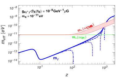
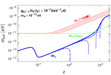
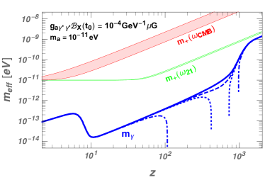
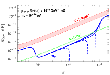
Figure 1: Evolution of the effective photon mass (blue) in the early Universe for $\omega=\omega_{21}$(solid), $T$(dashed), $4T$(dotted), $10T$(dash-dotted), where $T$ is the CMB temperature, and also the effective mass of the dark sector mass eigenstate $\phi_{+}$ with $\omega=\omega_{21}$ (green) and $\omega$ in the COBE-FIRAS frequency range $[1.2T,\,11.2T]$ (red). The upper left panel is for $(m_{a},g_{a\gamma^{\prime}\gamma^{\prime}}{\cal B}_{X})=(10^{-11}\,{\rm eV},10^{-9}\,{\rm GeV}^{-1}\mu{\rm G})$ for which both the CMB and 21 cm photon experience a resonant conversion, the lower left panel is for $(10^{-11}\,{\rm eV},\,10^{-4}\,{\rm GeV}^{-1}\mu{\rm G})$ for which neither of CMB and 21 cm photon experiences a resonant conversion, and finally the upper and lower right panels are for $(10^{-11}\,{\rm eV},10^{-7}\,{\rm GeV}^{-1}\mu{\rm G})$ and $(10^{-16}\,{\rm eV},10^{-7}\,{\rm GeV}^{-1}\mu{\rm G})$, respectively, for which the 21 cm photon experiences a resonant conversion, while the CMB does not.

In the limit $g_{a\gamma^{\prime}\gamma^{\prime}}{\cal B}_{X}\omega\ll m_{a}^{2}$, the dark sector mixing angle $\theta_{D}\ll 1$. In this limit, the propagation eigenstates are given by

$$\phi_{+}\simeq a,\quad\phi_{-}\simeq X_{\parallel},$$ (37)

with the mass eigenvalues

$$m_{+}^{2}\simeq m_{a}^{2},\quad m_{-}^{2}\simeq-\theta_{D}^{2}m_{a}^{2}.$$ (38)

Then resonant conversion can take place between $\gamma$ and $\phi_{+}$ when $m_{\gamma}^{2}(z)=m_{+}^{2}$ in the early Universe. Since $m_{+}^{2}\simeq m_{a}^{2}$ is approximately a constant, this is essentially same as the well known $\gamma$-$a$ conversion induced by the conventional ALP coupling $g_{a\gamma\gamma}aF\tilde{F}$ in background magnetic field $B$, but with $g_{a\gamma\gamma}B$ replaced by $g_{a\gamma\gamma^{\prime}}{\cal B}_{X}$. Obviously, in this case the resonance condition $m_{\gamma}^{2}(z)=m_{+}^{2}\simeq m_{a}^{2}$ can be fulfilled for $\omega=\omega_{21}$ and $20<z<1700$ only for

$$m_{a}={\cal O}(10^{-14}-10^{-9})\,\,{\rm eV}.$$ (39)

For subsequent discussions, it is convenient to define

$$\omega_{L}(t_{0})=\frac{1}{(1+z_{\rm res})^{3}}\frac{m_{a}^{2}}{g_{a\gamma^{\prime}\gamma^{\prime}}{\cal B}_{X}(t_{0})},$$ (40)

where $t_{0}$ denotes the present Universe and $z_{\rm res}$ is the red-shift at the time $t=t_{\rm res}$ when the resonance condition $m_{\gamma}^{2}=m_{+}^{2}\simeq m_{a}^{2}$ is met. Note that for $m_{a}<1.6\times 10^{-14}$ eV, such resonance condition can not be fulfilled, so $\omega_{L}$ for $m_{a}<1.6\times 10^{-14}$ eV is fixed to the value at $m_{a}=1.6\times 10^{-14}~{}{\rm eV}$ and $z_{\rm res}=11$. Then the resonant conversion between $\gamma$ and $\phi_{+}\simeq a$ takes place in the small dark sector mixing regime for the ALP mass range (39) and the frequency

$$\omega\,\ll\,\omega_{L},$$ (41)

where we assume that the background dark photon gauge field is generated before $t_{\rm res}$ and subsequently red-shifted as ${\cal B}_{X}(t_{0})={\cal B}_{X}(t)/(1+z)^{2}$. The corresponding resonant conversion probability can be obtained from Eqs. (90) and (91) by inserting $m_{\rm mix}^{2}=g_{a\gamma\gamma^{\prime}}{\cal B}_{X}\omega$ and $m_{\phi}^{2}=m_{a}^{2}$, which results in

$$P_{\gamma\leftrightarrow\phi_{+}\simeq a}(\omega\ll\omega_{L})\,\simeq\,1-p_{\rm res}\,\simeq\,1-\left.\exp\left(-r\frac{\pi g_{a\gamma\gamma^{\prime}}^{2}{\cal B}_{X}^{2}\omega}{m_{a}^{2}}\right)\right|_{t=t_{\rm res}},$$ (42)

where

$$r^{-1}={|d\ln(m_{\gamma}^{2}/m_{+}^{2})/{dt}|_{t=t_{\rm res}}}={\cal O}\left(1-10\right)\times H(t_{\rm res})$$ (43)

for the Hubble expansion rate $H(t)$. In the parameter region giving $rg_{a\gamma\gamma^{\prime}}^{2}{\cal B}_{X}^{2}\omega/m_{a}^{2}\gtrsim 1$, the conversion probability is close to unity and nearly independent of the photon frequency $\omega$. On the other hand, in the other limit with $rg_{a\gamma\gamma^{\prime}}^{2}{\cal B}_{X}^{2}\omega/m_{a}^{2}\ll 1$, the conversion probability is small and proportional to the photon frequency as

$$P_{\gamma\leftrightarrow\phi_{+}\simeq a}(\omega\ll\omega_{L})\,\simeq\,r\frac{\pi g_{a\gamma\gamma^{\prime}}^{2}{\cal B}_{X}^{2}\omega}{m_{a}^{2}}.$$ (44)

As the dark photon does not participate in resonant conversion in this case, the photon density spectrum is reshaped mainly by the $\gamma$-$a$ conversion as

$$\frac{dn_{\gamma}}{d\omega}\quad\rightarrow\quad\frac{dn_{\gamma}}{d\omega}\times\left(P_{\gamma\rightarrow\gamma}\right)_{\omega\ll\omega_{L}}+\frac{dn_{a}}{d\omega}\times\left(P_{\gamma\rightarrow\phi_{+}\simeq a}\right)_{\omega\ll\omega_{L}}\,,$$ (45)

where $P_{\gamma\rightarrow\gamma}\,\simeq\,1-P_{\gamma\rightarrow\phi_{+}\simeq a}$ is the photon survival probability.

2.2 Large dark sector mixing

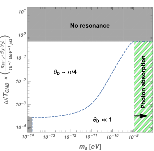
Figure 2: Parameter regions for small dark sector mixing, large dark sector mixing, and no resonance. The dotted curve corresponds to $\tan 2\theta_{D}=1$, and the gray area does not allow the resonance condition $m_{\gamma}^{2}=m_{\pm}^{2}$ to be fulfilled.

The most interesting feature of our scheme appears in the large dark sector mixing regime with $\tan 2\theta_{D}=2g_{a\gamma^{\prime}\gamma^{\prime}}{\cal B}_{X}\omega/m_{a}^{2}\gg 1$. In such case, the propagation eigenstates are given by the nearly maximal mixtures of ALP and dark photon,

$$\phi_{\pm}\simeq\frac{X_{\parallel}\pm a}{\sqrt{2}}$$ (46)

with the mass eigenvalues

$$m_{\pm}^{2}\simeq\pm m_{\gamma^{\prime}a}^{2}=\pm g_{a\gamma^{\prime}\gamma^{\prime}}{\cal B}_{X}\omega\,.$$ (47)

In this case also, the primary resonance conversion takes place between $\gamma$ and $\phi_{+}$ when $m_{\gamma}^{2}=m_{+}^{2}$. However there is a key difference from the small dark sector mixing case. The mass eigenvalue $m_{+}^{2}$ in the large mixing case is red-shifted as $(1+z)^{3}$ in the expanding Universe, while it is approximately constant in the small mixing case.

More specifically, $m_{\pm}^{2}$ in the limit $\tan 2\theta_{D}\gg 1$ is red-shifted like $\omega_{\rm pl}^{2}\propto n_{e}\propto(1+z)^{3}$ when the hydrogen ionization fraction $X_{e}$ is constant, e.g. before the recombination and after the re-ionization. (See for instance the cosmic evolution of $m_{+}$ and $m_{\gamma}$ in Fig. 1.) By virtue of this coincidence, if $g_{a\gamma^{\prime}\gamma^{\prime}}{\cal B}_{X}\omega$ is large enough, $m_{+}^{2}>\omega_{\rm pl}^{2}$ over the whole evolution history, so the resonance condition $m_{\gamma}^{2}=m_{+}^{2}$ can never be fulfilled as in the case of $m_{+}(\omega_{\rm CMB})$ in the upper right panel and lower two panels of Fig. 1. One easily finds that this happens for

$$\omega(t_{0})>\omega_{c}(t_{0})=1.4\times 10^{-4}~{}{\rm eV}\left(\frac{10^{-7}~{}{\rm GeV}^{-1}\mu{\rm G}}{g_{\gamma^{\prime}\gamma^{\prime}}{\cal B}_{X}(t_{0})}\right)\,,$$ (48)

which corresponds to the upper gray region in Fig. 2. In Fig. 2, we depict also the curve for $\tan 2\theta_{D}=1$ which splits the parameter space into the two regions, the large dark sector mixing region (upper) and the small dark sector mixing region (lower).

If the critical frequency $\omega_{c}$ is lower than the CMB frequencies $\omega=[1.2T,\,11.2T]$ probed by the COBE-FIRAS Fixsen:1996nj , i.e.

$$\omega_{c}(t_{0})<2.84\times 10^{-4}~{}{\rm eV}$$ (49)

or equivalently

$$g_{a\gamma^{\prime}\gamma^{\prime}}{\cal B}_{X}(t_{0})>4.6\times 10^{-8}~{}{\rm GeV}^{-1}\mu{\rm G}\,,$$ (50)

there could be no resonant conversion for the CMB in the COBE-FIRAS frequencies as in the upper right panel and lower two panels of Fig. 1, which is one of the most interesting features of our scheme. We note that once the above condition is satisfied, which assures that $\phi_{+}$ does not experience a resonance conversion to $\gamma$ in the COBE-FIRAS frequency range, $\phi_{-}$ also can not have a resonance conversion to $\gamma$ in the same frequency range. Even though $m_{\gamma}^{2}$ for $\omega>3.8\,T$ becomes negative during certain period as in the case of dotted and dash-dotted blue curves in Fig. 1, its absolute value is not large enough to satisfy $m_{\gamma}^{2}=m_{-}^{2}\simeq-g_{a\gamma^{\prime}\gamma^{\prime}}{\cal B}_{X}\omega$ for the COBE-FIRAS frequencies and $g_{a\gamma^{\prime}\gamma^{\prime}}{\cal B}_{X}$ satisfying (50). Yet, there can be non-resonant conversion between CMB and $\phi_{\pm}$. As there is no resonant conversion, we can set $p_{\rm res}=0$ in (90), and find the corresponding non-resonant conversion probability

$$P_{\gamma\leftrightarrow a,\gamma^{\prime}}(\omega>\omega_{c})\,\simeq\,\frac{1}{2}\frac{g^{2}_{a\gamma\gamma^{\prime}}}{g^{2}_{a\gamma^{\prime}\gamma^{\prime}}}$$ (51)

for $g_{a\gamma\gamma^{\prime}}/g_{a\gamma^{\prime}\gamma^{\prime}}\ll 1$.

Due to the rapid reduction of the hydrogen ionization fraction $X_{e}$, the effective photon mass $m_{\gamma}^{2}$ is more rapidly red-shifted than $m_{+}^{2}\simeq g_{a\gamma^{\prime}\gamma^{\prime}}{\cal B}_{X}\omega\propto(1+z)^{3}$ right after the recombination (see Fig. 1). As a consequence, there exists an intermediate frequency range over which the resonance condition $m_{\gamma}^{2}=m_{+}^{2}$ can be fulfilled in the large dark sector mixing regime as in the case of $m_{+}(\omega_{21})$ in the upper and lower right panels of Fig. 1. Such frequency range is given by

$$\omega_{L}(t_{0})\,<\,\omega(t_{0})\,<\,\omega_{c}(t_{0}),$$ (52)

where $\omega_{c}$ is given in (48) and $\omega_{L}$ is given in (40). In Fig. 2, the parameter region above the dotted curve but below the upper gray area corresponds to this intermediate frequency range. In fact, in this case there can be a resonant conversion between $\gamma$ and $\phi_{+}$ during the period $20<z<1700$ even when $m_{a}\ll m_{\gamma}(z=20)\sim 10^{-14}$ eV. This is because the resonance conversion occurs through the effective mass $m^{2}_{+}\simeq g_{a\gamma^{\prime}\gamma^{\prime}}{\cal B}_{X}\omega$ satisfying $m_{+}^{2}=m_{\gamma}^{2}$ even when $m_{a}\ll 10^{-14}$ eV. In such case, as shown in the lower right panel of Figure. 1, there is an additional resonant conversion at lower redshift $z<10$. However this later conversion is less significant than the earlier one occurring at $z\sim 10^{3}$ because it is less adiabatic.

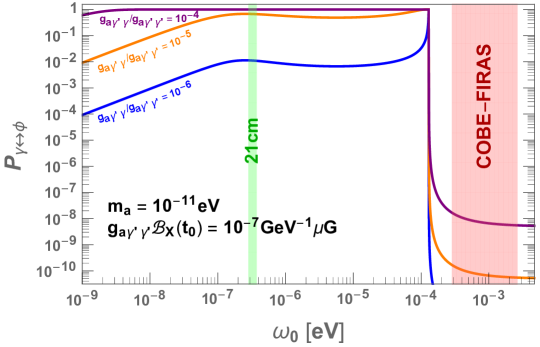
Figure 3: Spectral dependence of the resonant conversion probability $P_{\gamma\leftrightarrow\phi_{+}}$ for the parameter choice of $m_{a}=10^{-11}{\rm eV}$, $g_{a\gamma^{\prime}\gamma^{\prime}}{\cal B}_{X}(t_{0})=10^{-7}{\rm GeV}^{-1}\mu{\rm G}$, and $g_{a\gamma\gamma^{\prime}}/g_{a\gamma^{\prime}\gamma^{\prime}}=10^{-6}$ (blue), $10^{-5}$ (orange), and $10^{-4}$ (purple). The COBE-FIRAS frequency range corresponds to the red-colored region where the resonance condition can not be fulfilled, and therefore the conversion occurs through tiny non-resonant process. The conversion probability $P_{\gamma\leftrightarrow\phi_{+}}\propto\omega$ in the low frequency regime with $\omega<\omega_{L}$, nearly flat over $\omega_{L}<\omega<\omega_{c}$, and then sharply drop to a small non-resonant conversion probability $P_{\gamma\leftrightarrow\phi_{+}}\simeq g_{a\gamma\gamma^{\prime}}^{2}/2g_{a\gamma^{\prime}\gamma^{\prime}}^{2}$ at $\omega>\omega_{c}$.

Applying Eqs. (90) and (91) for the mass parameters

$$m_{\phi}^{2}\simeq m_{\gamma^{\prime}a}^{2}=g_{a\gamma^{\prime}\gamma^{\prime}}{\cal B}_{X}\omega,\quad m_{\rm mix}^{2}=-\frac{m_{\gamma a}^{2}}{\sqrt{2}}=-\frac{g_{a\gamma\gamma^{\prime}}{\cal B}_{X}\omega}{\sqrt{2}},$$ (53)

while assuming $g_{a\gamma\gamma^{\prime}}\ll g_{a\gamma^{\prime}\gamma^{\prime}}$, we find that the conversion probability in the intermediate frequency range is given by

$$P_{\gamma\leftrightarrow a,\gamma^{\prime}}(\omega_{L}<\omega<\omega_{c})\,\simeq\,1-p_{\rm res}\,\simeq\,1-\left.\exp\left(-r\frac{\pi g_{a\gamma\gamma^{\prime}}^{2}{\cal B}_{X}}{2g_{a\gamma^{\prime}\gamma^{\prime}}}\right)\right|_{t=t_{\rm res}},$$ (54)

where

$$r^{-1}={|d\ln(m_{\gamma}^{2}/m_{+}^{2})/{dt}|_{t=t_{\rm res}}}={\cal O}\left(1-10\right)\times H(t_{\rm res}).$$ (55)

Note that the resonance conversion in this regime typically occurs right after the recombination when $X_{e}$ rapidly decreases as in the case of $m_{+}(\omega_{21})$ in the upper and lower right panels of Fig. 1. As a consequence, the frequency-dependence of the conversion probability is weakened and becomes approximately $\omega$-independent as in (54), which is another interesting feature of our scheme. We note also that the conversion probability is quite sensitive to the ALP coupling ratio $g_{a\gamma\gamma^{\prime}}/g_{a\gamma^{\prime}\gamma^{\prime}}$. The above resonance conversion between $\gamma$ and $\phi_{+}$ in the large dark sector mixing regime results in the modification of the photon density spectrum as

$$\frac{dn_{\gamma}}{d\omega}\quad\rightarrow\quad\frac{dn_{\gamma}}{d\omega}\times\left(P_{\gamma\rightarrow\gamma}\right)_{\omega>\omega_{L}}+\frac{1}{2}\left(\frac{dn_{a}}{d\omega}+\frac{dn_{\gamma^{\prime}}}{d\omega}\right)\times\left(P_{\gamma\leftrightarrow a,\gamma^{\prime}}\right)_{\omega>\omega_{L}}\,,$$ (56)

where the factor $1/2$ originates from the large mixing between dark photon and ALP. Note that although $\gamma^{\prime}$ is exactly massless in the vacuum, it has a large mixture with the (approximate) mass eigenstate $\phi_{+}$ when $g_{a\gamma^{\prime}\gamma^{\prime}}{\cal B}_{X}\omega\gtrsim m_{a}^{2}$, so actively participates in the resonant conversion to $\gamma$ in the early Universe.

In Fig. 3, we depict the spectral dependence of the conversion probability $P_{\gamma\leftrightarrow\phi_{+}}$ for $m_{a}=10^{-11}\,{\rm eV}$, $g_{a\gamma^{\prime}\gamma^{\prime}}{\cal B}_{X}=10^{-7}~{}{\rm GeV}^{-1}\mu{\rm G}$, and three different values of $g_{a\gamma\gamma^{\prime}}/g_{a\gamma^{\prime}\gamma^{\prime}}=10^{-4}$, $10^{-5}$ and $10^{-6}$. As was anticipated from (42) and (44), in the low frequency regime with $\omega\ll\omega_{L}$, which corresponds to the small dark sector mixing regime, the conversion probability has a nearly flat spectral dependence when it is close to unity, which is the case for $g_{a\gamma\gamma^{\prime}}/g_{a\gamma^{\prime}\gamma^{\prime}}=10^{-4}$, but grows as $P_{\gamma\leftrightarrow\phi_{+}}\propto\omega$ when it is small, which is the case for $g_{a\gamma\gamma^{\prime}}/g_{a\gamma^{\prime}\gamma^{\prime}}=10^{-5},10^{-6}$. As (54) indicates, the conversion probability is approximately flat over the intermediate frequency range $\omega_{L}<\omega<\omega_{c}$ regardless of the value of $g_{a\gamma\gamma^{\prime}}/g_{a\gamma^{\prime}\gamma^{\prime}}$, and finally sharply drops to a small non-resonant conversion probability $P_{\gamma\leftrightarrow\phi_{+}}\simeq g_{a\gamma\gamma^{\prime}}^{2}/2g_{a\gamma^{\prime}\gamma^{\prime}}^{2}$ at $\omega>\omega_{c}$. For the chosen values of $m_{a}$ and $g_{a\gamma^{\prime}\gamma^{\prime}}{\cal B}_{X}$, we have $\omega_{\rm CMB}>\omega_{c}$ (red-colored) and $\omega_{L}<\omega_{21}<\omega_{c}$ (green-colored). Fig. 3 shows that our scheme can give a sizable conversion of dark radiations, either ALPs or dark photons, to 21 cm photons, even with a probability close to unity, while avoiding dangerous CMB distortions.

3 Implication for the EDGES 21 cm signal

The ALP-photon-dark photon oscillation discussed in the previous section provides an appealing mechanism to explain the recent tentative observation by the EDGES experiment of an anomalously strong absorption signal of 21 cm photons Bowman:2018yin . In this section, we examine this possibility in more detail.

To explain the EDGES anomaly by a resonant conversion of $\phi$ into 21 cm photons Pospelov:2018kdh ; Moroi:2018vci , we need a conversion probability

$$P_{\phi\rightarrow\gamma}\,\sim\,\frac{10^{-9}}{f_{\phi}^{\rm 21cm}\Delta N_{\rm eff}^{\phi}},$$ (57)

where $\Delta N_{\rm eff}^{\phi}$ denotes the energy density of $\phi$ parametrized by the effective number of neutrino species and $f_{\phi}^{\rm 21cm}$ is the energy fraction in the 21 cm frequency range. Since the energy density of total dark radiation is bounded as $\Delta N_{\rm eff}{\;\raise 1.29167pt\hbox{$<$\kern-7.5pt\raise-4.73611pt\hbox{$\sim$}}\;}0.3$ Ade:2015xua , the conversion probability has to be at least of the order of $10^{-8}$ to explain the EDGES anomaly. For the scenarios proposed Pospelov:2018kdh ; Moroi:2018vci , the parameter region giving $P_{\phi\rightarrow\gamma}\gtrsim 10^{-8}$ is severely limited by a variety of phenomenological constraints. As a consequence, either only a tiny parameter region remains to be viable, or the viable parameter region may suffer from a fine-tuning problem. For instance, for the dark photon scenario of Pospelov:2018kdh , generating the tiny dark photon mass $m_{\gamma^{\prime}}={\cal O}(10^{-14}-10^{-9})$ eV and also small kinetic mixing $\epsilon<10^{-5}$ in the UV completion of the model may cause a naturalness problem. As for the ALP scenario of Moroi:2018vci , we combine in Appendix C the CMB distortion constraint with the additional constraints from the absence of $\gamma$-ray burst associated with SN1987A Payez:2014xsa and the upper bound on the primordial background magnetic field to avoid an overheating of baryons which would wash away the EDGES signal Minoda:2018gxj . We then find that the parameter region giving $P_{\phi\rightarrow\gamma}\gtrsim 10^{-7}$ for the ALP mass $m_{a}=10^{-14}-10^{-9}$ eV is fully excluded by these constraints. If the primordial background magnetic field nearly saturates its upper bound $B_{0}\lesssim 0.1$ nG, a tiny parameter region can give $P_{\phi\rightarrow\gamma}\gtrsim 10^{-8}$, while satisfying the observational constraints. This means that the ALP scheme of Moroi:2018vci can explain the EDGES anomaly only when both the ALP dark radiation and the primordial background magnetic field nearly saturate their upper bounds, i.e. $f_{\phi}^{\rm 21cm}\Delta N_{\rm eff}^{\phi}\sim 0.1$ and $B_{0}\sim 0.1$ nG. On the other hand, our scenario can give a large conversion probability even close to unity, while satisfying the observational constraints and also without causing a fine-tuning problem. As a result, in our scheme even a small amount of dark radiation at the 21 cm frequency range, e.g. $f_{\phi}^{\rm 21cm}\Delta N_{\rm eff}^{\phi}\sim 10^{-9}$, can give an enough boost to heat up the 21 cm photons, so can explain the EDGES anomaly.

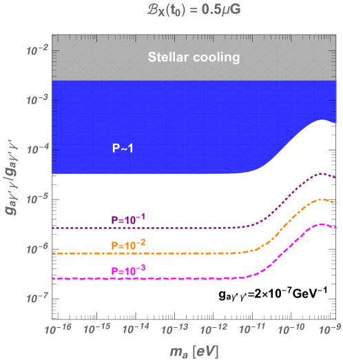
Figure 4: Contour of the resonant conversion probability $P_{\gamma\leftrightarrow\phi_{+}}\simeq 1$ (blue region), $10^{-1}$ (purple), $10^{-2}$ (orange), $10^{-3}$ (magenta) for 21 cm photons. Here we take $g_{a\gamma^{\prime}\gamma^{\prime}}=2\times 10^{-7}\,{\rm GeV}^{-1}$ and ${\cal B}_{X}(t_{0})=0.5\,\mu{\rm G}$. The gray region is excluded by the stellar cooling bound $g_{a\gamma\gamma^{\prime}}<5\times 10^{-10}\,{\rm GeV}^{-1}$.

Let us now identify the model parameter region of our scheme which can explain the EDGES anomaly while satisfying the observational constraints. To have a resonant conversion of dark radiations to 21 cm photons at $20<z<1700$, we first need

$$m_{a}<10^{-9}\,{\rm eV}.$$ (58)

Note that in our scheme such resonance conversion can occur even when $m_{a}\ll m_{\gamma}(z\simeq 20)\sim 10^{-14}$ eV as long as the effective DR mass fulfils the resonance condition $m_{+}^{2}\simeq g_{a\gamma^{\prime}\gamma^{\prime}}{\cal B}_{X}\omega=m_{\gamma}^{2}$ for $\omega=\omega_{21}$ and $20<z<1700$. As was noticed in the previous section, we can avoid a resonant conversion at the CMB frequencies, while having a large conversion at the 21 cm frequency, by arranging the model parameters to have $\omega_{21}<\omega_{c}<\omega_{\rm CMB}$, where $\omega_{c}$ is the critical frequency given by (48). This can be achieved for

$$4.6\times 10^{-8}\,{\rm GeV}^{-1}\mu{\rm G}\,<\,g_{a\gamma^{\prime}\gamma^{\prime}}{\cal B}_{X}\,<\,3.7\times 10^{-5}\,{\rm GeV}^{-1}\mu{\rm G},$$ (59)

where we used $\omega_{\rm CMB}\simeq 1.2\,T_{\rm CMB}$ which corresponds to the lowest CMB frequency probed by the COBE-FIRAS. As the background dark photon gauge field $\langle X_{\mu\nu}\rangle\propto(1+z)^{2}$, its energy density is a part of the total dark radiation energy density which is bounded as $\Delta N_{\rm eff}<0.3$ Ade:2015xua . This requires that ${\cal B}_{X}\lesssim 1~{}\mu{\rm G}$, and then the above condition implies that we need

$$g_{a\gamma^{\prime}\gamma^{\prime}}\,\gtrsim\,4\times 10^{-8}\,{\rm GeV}^{-1}.$$ (60)

We note that practically there is no observational constraint on $g_{a\gamma^{\prime}\gamma^{\prime}}$, so in principle $g_{a\gamma^{\prime}\gamma^{\prime}}$ can be significantly bigger than the above lower bound. Absence of a resonant conversion at CMB frequencies does not guarantee that the scheme is free from CMB distortion. To be compatible with the COBE-FIRAS CMB observation, we need to suppress the non-resonant conversion probability (51) as

$$P_{\gamma\leftrightarrow a,\gamma^{\prime}}(\omega\sim\omega_{\rm CMB})\,\simeq\,\frac{1}{2}\frac{g^{2}_{a\gamma\gamma^{\prime}}}{g^{2}_{a\gamma^{\prime}\gamma^{\prime}}}\lesssim 10^{-4},$$ (61)

which requires

$$\frac{g_{a\gamma\gamma^{\prime}}}{g_{a\gamma^{\prime}\gamma^{\prime}}}\lesssim 1.4\times 10^{-2}.$$ (62)

The conversion probability $P_{\gamma\leftrightarrow\phi^{+}}$ given in (42) and (54) indicates that the ALP coupling ratio $g_{a\gamma\gamma^{\prime}}/g_{a\gamma^{\prime}\gamma^{\prime}}$ is a key parameter to determine the size of the conversion rate at $\omega=\omega_{21}$. In Fig. 4, we plot the contours of $P_{\gamma\leftrightarrow\phi^{+}}(\omega=\omega_{21})$ in the parameter space $(m_{a},g_{a\gamma\gamma^{\prime}}/g_{a\gamma^{\prime}\gamma^{\prime}})$ for $g_{a\gamma^{\prime}\gamma^{\prime}}=2\times 10^{-7}\,{\rm GeV}^{-1}$ and ${\cal B}_{X}=0.5$ $\mu$G. Our result shows that the conversion probability can be close to unity over a wide range of parameter space satisfying the observational constraints. This allows that our scheme can provide a viable explanation of the EDGES anomaly even with a small amount of DR ($\phi=a$ or $\gamma^{\prime}$) at the 21 cm frequency range, e.g. $f_{\phi}^{\rm 21cm}\Delta N_{\rm eff}^{\phi}\sim 10^{-9}$.

A key ingredient of our scheme is the existence of a primordial background dark photon gauge field $\langle X_{\mu\nu}\rangle=(\vec{E}_{X},\vec{B}_{X})$. As was demonstrated in Choi:2018dqr , even a large $\langle X_{\mu\nu}\rangle$ close to the upper bound $\sim 1$ $\mu$G can be generated by an ultra-light ALP $\varphi$ which couples to the dark photon gauge field through

$$\frac{1}{4}g_{\varphi\gamma^{\prime}\gamma^{\prime}}\varphi X_{\mu\nu}\tilde{X}^{\mu\nu}.$$ (63)

In Appendix B, we provide an explicit scheme to generate the necessary $\langle X_{\mu\nu}\rangle$ based on the results of Choi:2018dqr .

Another key ingredient of our scheme to explain the EDGES anomaly is the DR composed of $a$ or $\gamma^{\prime}$ with an energy density (in the 21 cm frequency range) satisfying

$$f_{\phi}^{\rm 21cm}\Delta N_{\rm eff}^{\phi}\,\sim\,\frac{10^{-9}}{P_{\phi\rightarrow\gamma}}.$$ (64)

For the origin of such DR, we can use the mechanisms proposed in Pospelov:2018kdh ; Moroi:2018vci utilizing the moduli or saxion decays into ALPs or the decays of another ALP (constituting the dark matter) to dark photons. Alternatively one can adopt the mechanism of Choi:1996vz utilizing the decays of flaton to either ALPs or dark photons. As it is rather straightforward to apply the results of Pospelov:2018kdh ; Moroi:2018vci to our case, we do not provide a separate discussion on the generation of DR satisfying the condition (64).

As indicated by (60) and (62), our scheme requires a hierarchical pattern of ALP couplings:

$$g_{a\gamma\gamma},\,g_{a\gamma\gamma^{\prime}}\,\ll\,g_{a\gamma^{\prime}\gamma^{\prime}}.$$ (65)

There can be a variety of ways to achieve such hierarchical ALP couplings without causing a fine tuning problem. One option is that the PQ-charged massive fermions in the underlying UV model are charged only under $U(1)_{X}$, while there exist additional PQ-singlet massive fermions charged under both $U(1)_{X}$ and the SM hypercharge $U(1)_{Y}$ Kaneta:2016wvf ; Kaneta:2017wfh . Then the loops of PQ-singlet massive fermions induces a kinetic mixing $\varepsilon={\cal O}(eg_{X}/16\pi^{2})={\cal O}(10^{-3}-10^{-2})$ between $X_{\mu\nu}$ and $F_{\mu\nu}$, while the loops of PQ-charged massive fermions generates the ALP coupling $g_{a\gamma^{\prime}\gamma^{\prime}}$ without generating $g_{a\gamma\gamma},\,g_{a\gamma\gamma^{\prime}}$ in the original field basis. Then, rotating away the kinetic mixing by an appropriate field redefinition, we obtain the ALP couplings

$$g_{a\gamma\gamma}\sim\epsilon g_{a\gamma\gamma^{\prime}}\sim\epsilon^{2}g_{a\gamma^{\prime}\gamma^{\prime}}.$$ (66)

Alternatively one may use the clockwork mechanism of Choi:2014rja ; Choi:2015fiu ; Kaplan:2015fuy to generate a hierarchical pattern of ALP couplings as in Higaki:2015jag ; Farina:2016tgd ; Agrawal:2017cmd , which can give even a bigger hierarchy among the ALP couplings. Note that the above pattern of ALP couplings is in good accordance with the astrophysical constraints

$$g_{a\gamma\gamma^{\prime}}<5\times 10^{-10}{\rm GeV}^{-1},\quad g_{a\gamma\gamma}<5\times 10^{-12}{\rm GeV}^{-1}$$ (67)

which are deduced from the star cooling due to the plasmon decay $\gamma_{\rm pl}\rightarrow a\gamma^{\prime}$ Choi:2018mvk and the absence of $\gamma$-ray burst associated with SN1987A Payez:2014xsa .

4 Conclusion

In this paper, we examined the ALP-photon-dark photon oscillations in background dark photon gauge field, while focusing on the resonant conversion between the photon and a dark radiation composed of ALPs and dark photons in the early Universe. We find that the corresponding conversion probability reveals an interesting spectral feature which allows strong conversion at low frequency domain, but has negligible conversion at high frequencies above certain critical frequency which is determined by the ALP coupling to dark photon and the strength of background dark photon gauge field. We then utilize this feature to heat up the 21 cm photons without affecting the Cosmic Microwave Background, which may explain the recent tentative observation by the EDGES experiment of an anomalously strong absorption signal of 21 cm photons. We find that our scheme can explain the EDGES anomaly over a wide range of parameter space, while satisfying the observational constraints and also without causing a naturalness problem.

Appendix A A brief review of resonant conversion between photon and dark radiation

Here we briefly review the cosmological resonant conversion between the photon $\gamma$ and a light hidden sector particle $\phi$ such as ALP or dark photon, which is a straightforward generalization of the well known Mikheyev-Smirnov-Wolfenstein (MSW) effect in neutrino physics Wolfenstein:1977ue ; Mikheev:1986gs ; Mikheev:1986wj . For this, let us consider the effective mass-square matrix of $\gamma$ and $\phi$ in generic time-dependent environment:

$$\mathcal{M}^{2}=\left[\begin{tabular}[]{cc}$m_{\gamma}^{2}$&$m_{\rm mix}^{2}$\\ $m_{\rm mix}^{2}$&$m_{\rm\phi}^{2}$\end{tabular}\right]\,,$$ (70)

where $m_{\gamma}$ is the effective photon mass induced by the scattering off the ambient medium, and $m_{\rm mix}$ describes the mixing induced by an appropriate coupling of $\phi$ to the photon. The evolution equation for relativistic propagation of $\gamma$ and $\phi$ is given by

$$\left[i\frac{d}{dt}-\frac{1}{2\omega}\mathcal{M}^{2}\right]\left(\begin{array}[]{c}\gamma\\ \phi\end{array}\right)=0\,,$$ (73)

where $\omega$ is the energy of the state. Here we are interested in the case that ${\cal M}^{2}$ varies in time due to the expansion of the early universe.

To proceed, one may rewrite the above evolution equation in the instantaneous mass eigenbasis $(\psi_{+},\psi_{-})$ as

$$\left[i\frac{d}{dt}-\left(\begin{array}[]{cc}\frac{1}{2\omega}(m_{\gamma}^{2}+m_{\phi}^{2})+\Delta_{\rm osc}&-i\frac{d\chi}{dt}\\ i\frac{d\chi}{dt}&\frac{1}{2\omega}(m_{\gamma}^{2}+m_{\phi}^{2})-\Delta_{\rm osc}\end{array}\right)\right]\left(\begin{array}[]{c}\psi_{+}\\ \psi_{-}\end{array}\right)=0\,.$$ (78)

where

$$\left(\begin{array}[]{c}\psi_{+}\\ \psi_{-}\end{array}\right)=\left(\begin{array}[]{cc}\cos\chi&-\sin\chi\\ \sin\chi&\cos\chi\end{array}\right)\left(\begin{array}[]{c}\gamma\\ \phi\end{array}\right)\,,$$ (85)

and the instantaneous mixing angle and oscillation frequency are given by

$$\tan 2\chi=\frac{2m_{\rm mix}^{2}}{m_{\gamma}^{2}-m_{\phi}^{2}},\quad\Delta_{\rm osc}=\frac{\sqrt{\left(m_{\gamma}^{2}-m_{\phi}^{2}\right)^{2}+4m_{\rm mix}^{4}}}{4\omega}.$$ (86)

The above evolution equation indicates that the transition between $\psi_{+}$ and $\psi_{-}$ is determined by the adiabaticity parameter

$$\gamma_{\rm ad}=\frac{\Delta_{\rm osc}}{|d\chi/dt|},$$ (87)

which is large in the adiabatic limit $|d\chi/dt|\ll\Delta_{\rm osc}$. In our case, the time variance of the mixing angle $\chi$ originates from the expansion of the universe. Then, in the small mixing regime with $\sin\chi\simeq|m_{\rm mix}^{2}/(m_{\phi}^{2}-m_{\gamma}^{2})|\ll 1$, we have $d\chi/dt={\cal O}(H\sin\chi)$, where $H$ is the Hubble expansion rate, while $d\chi/dt={\cal O}(H\times{\rm Max}(m_{\phi}^{2},m_{\gamma}^{2})/m_{\rm mix}^{2})$ in the large mixing regime with $|m_{\rm mix}^{2}/(m_{\phi}^{2}-m_{\gamma}^{2})|\gg 1.$

Here we are concerned with the conversion of an initial photon (or $\phi$) at $t_{i}$ to the hidden sector particle $\phi$ (or photon) in the final state at $t_{f}$. We can then consider two distinctive cases. The first case is that there occurs a sign flip of $m_{\gamma}^{2}-m_{\phi}^{2}$ during the evolution, e.g. $m_{\gamma}^{2}(t_{i})>m_{\phi}^{2}(t_{i})$, but $m_{\gamma}^{2}(t_{f})<m_{\phi}^{2}(t_{f})$, so there exists a resonance point where

$$m^{2}_{\gamma}(t_{\rm res})=m^{2}_{\phi}(t_{\rm res})\quad(t_{i}<t_{\rm res}<t_{f}).$$ (88)

The other case is that $m_{\gamma}^{2}(t)>m_{\phi}^{2}(t)$ over the entire evolution from $t_{i}$ to $t_{f}$, so there is no resonant point in between. Note that $0<\chi_{i}<\frac{\pi}{4}$ and $\frac{\pi}{4}<\chi_{f}<\frac{\pi}{2}$, and therefore $\cos 2\chi_{f}\cos 2\chi_{i}<0$ for the first case, while $0<\chi_{i},\chi_{f}<\frac{\pi}{4}$ for the other case, yielding $\cos 2\chi_{f}\cos 2\chi_{i}>0$.

If the relevant time intervals such as $t_{f}-t_{\rm res}$ and $t_{\rm res}-t_{i}$ are much longer than the oscillation length $\Delta_{\rm osc}^{-1}$, one can take an average over the production and detection points. In the adiabatic limit that $d\chi/dt$ in the evolution equation (78) can be ignored, one easily finds the conversion probability averaged over the production and detection points is given by

$$P_{\gamma\leftrightarrow\phi} = \frac{1}{2}-\frac{1}{2}\cos 2\chi_{f}\cos 2\chi_{i},$$ (89)

where $\chi_{i}$ and $\chi_{f}$ denote the mixing angles at the production and detection points, respectively. One can now include the effects of nonzero $d\chi/dt$ in the evolution. In our case, $\gamma_{\rm ad}=\Delta_{\rm osc}/|d\chi/dt|={\cal O}(\Delta_{\rm osc}/H\sin\chi)\gg 1$ except near the resonance point. Then the effects of time-varying mixing angle can be included in the transition probability as Parke:1986jy

$$P_{\gamma\leftrightarrow\phi} = \frac{1}{2}-\left(\frac{1}{2}-p_{\rm res}\right)\cos 2\chi_{f}\cos 2\chi_{i}+{\cal O}\left(\frac{H^{2}\sin\chi^{2}}{\Delta_{\rm osc}^{2}}\right)\,,$$ (90)

where $p_{\rm res}$ is the probability for the level crossing between $\psi_{+}$ and $\psi_{-}$ at the resonance point, and the last term is an order of magnitude estimate of the transitions between $\psi_{+}$ and $\psi_{-}$ that occur outside the resonance region. In case that there is no resonance point during the evolution, one can simply set $p_{\rm res}=0$ to get the corresponding conversion probability.

If the resonance time interval is short enough that $m_{\gamma}^{2}-m_{\phi}^{2}$ can be approximated as a linear function of time, which holds for our case, one can use the Landau-Zener result to find Landau ; Zener:1932ws

$$p_{\rm res}=\exp\left(-\frac{\pi{\gamma_{\rm ad}}(t_{\rm res})}{2}\right)\,\simeq\,\left.\exp\left(-r\frac{\pi m_{\rm mix}^{4}}{\omega m_{\phi}^{2}}\right)\right|_{t=t_{\rm res}}\,,$$ (91)

where

$$r^{-1}=\left|\frac{d\ln(m_{\gamma}^{2}(t)/m_{\phi}^{2}(t))}{dt}\right|_{t=t_{\rm res}}\,=\,{\cal O}(1-10)\times H(t_{\rm res})\,.$$ (92)

In case that $\gamma_{\rm ad}(t_{\rm res})\gg 1$ and therefore the evolution is adiabatic even at the resonance point, the level crossing probability $p_{\rm res}$ is exponentially small, which results in a large transition probability as

$$P_{\gamma\leftrightarrow\phi}=\frac{1}{2}+\frac{1}{2}|\cos 2\chi_{f}\cos 2\chi_{i}|+{\cal O}\left(\frac{H^{2}\sin\chi^{2}}{\Delta_{\rm osc}^{2}},\exp\left(-\frac{\pi\gamma_{\rm ad}(t_{\rm res})}{2}\right)\right).$$ (93)

Note that $\cos 2\chi_{f}\cos 2\chi_{i}<0$ in this case. On the other hand, if $\gamma_{\rm ad}(t_{\rm res})\ll 1$, which means that adiabaticity is abruptly violated at the resonance point, the level crossing probability $p_{\rm res}$ is close to the unity and then the transition probability can be approximated as

$$P_{\gamma\leftrightarrow\phi}=\frac{1}{2}\left(1-|\cos 2\chi_{f}\cos 2\chi_{i}|\right)+\frac{\pi}{2}|\cos 2\chi_{f}\cos 2\chi_{i}|\gamma_{\rm ad}(t_{\rm res})+{\cal O}\left(\frac{H^{2}\sin\chi^{2}}{\Delta_{\rm osc}^{2}}\right),$$ (94)

In fact, in this case the initial and final mixing angles have small values as $\chi_{i}^{2},\chi_{f}^{2}<\gamma_{\rm as}(t_{\rm res})\ll 1$, so the conversion probability can be approximated by the following simple form:

$$P_{\gamma\leftrightarrow\phi}\,\simeq\,\frac{\pi\gamma_{\rm ad}(t_{\rm res})}{2}\,=\,\left.r\frac{\pi m_{\rm mix}^{4}}{\omega m_{\phi}^{2}}\right|_{t=t_{\rm res}},$$ (95)

where $r^{-1}=\left|d\ln(m_{\gamma}^{2}/m_{\phi}^{2})/{dt}\right|_{t=t_{\rm res}}\,=\,{\cal O}(1-10)\times H(t_{\rm res})$.

Appendix B Generation of background dark photon gauge field

To complete our scheme, we need an explanation for the origin of the primordial background dark photon gauge field $\langle X_{\mu\nu}\rangle$, Here we discuss an explicit scheme to generate the required $\langle X_{\mu\nu}\rangle=(\vec{E}_{X},\vec{B}_{X})$, which is based on the mechanism of Choi:2018dqr . For this, we introduce an additional ultra-light ALP $\varphi$ which couples to the massless dark photon gauge field $X_{\mu}$ as

$$\frac{1}{4}g_{\varphi\gamma^{\prime}\gamma^{\prime}}\varphi X_{\mu\nu}\tilde{X}^{\mu\nu}.$$ (96)

Around the time $t_{\rm osc}$ when the Hubble expansion rate $H(t_{\rm osc})\sim m_{\varphi}$, the ultra-light ALP $\varphi$ begins to oscillate as

$$\varphi\simeq\varphi_{i}\left(\frac{R(t)}{R(t_{\rm osc})}\right)^{-3/2}\cos\left(m_{\varphi}(t-t_{\rm osc})\right),$$ (97)

where $R(t)$ is the scale factor of the expanding Universe with the spacetime metric $ds^{2}=dt^{2}-R^{2}(t)d\vec{x}^{2}$. The oscillating $\varphi$ causes a tachyonic instability of $X_{\mu}$ through the ALP coupling (96) for the wave numbers $k\sim g_{\varphi\gamma^{\prime}\gamma^{\prime}}\dot{\varphi}$, thereby amplifies the quantum fluctuation of $X_{\mu}$ to a stochastic classical background field. For efficient amplification, $g_{\varphi\gamma^{\prime}\gamma^{\prime}}\varphi_{i}$ needs to be large enough to overcome the dilution by the Hubble expansion, but not too large to avoid a too strong friction which would forbid the oscillatory motion of $\varphi$. It was found in Kitajima:2017peg ; Choi:2018dqr ; Agrawal:2018vin that this can be achieved when

$$g_{\varphi\gamma^{\prime}\gamma^{\prime}}\varphi_{i}={\cal O}(10-100),$$ (98)

which will be assumed here. Then we can use the results of Choi:2018dqr to find that the amplified dark photon gauge field today is determined by the initial ALP misalignment as

$$|\vec{E}_{X}(t_{0})|\sim|\vec{B}_{X}(t_{0})|\sim 0.3\,\mu{\rm G}\left(\frac{\varphi_{i}}{10^{17}\,{\rm GeV}}\right),$$ (99)

while the red-shift $z_{*}$ at the time of amplification (production) and the coherent length $\lambda$ of the produced fields today are determined by the ALP mass as

$$z_{*}\,\sim\,10^{4}\bigg{(}\frac{m_{\varphi}}{10^{-25}\text{eV}}\bigg{)}^{1/2},\quad\lambda\,\sim\,3\,{\rm Mpc}\bigg{(}\frac{m_{\varphi}}{10^{-25}\text{eV}}\bigg{)}^{-1/2}.$$ (100)

This process leaves also a coherently oscillating ALP dark matter whose mass density is given by

$$\frac{\Omega_{\varphi}h^{2}}{0.12}\simeq 10^{-3}\,\bigg{(}\frac{m_{\varphi}}{10^{-25}\text{eV}}\bigg{)}^{1/2}\left(\frac{\varphi_{i}}{10^{17}\,{\rm GeV}}\right)^{2}.$$ (101)

The energy density of the produced $\vec{E}_{X}$ and $\vec{B}_{X}$ is red-shifted like a radiation energy density, so is bounded as $\Delta N^{X}_{\text{eff}}\leq 0.3$, where

$$\Delta N^{X}_{\text{eff}}\simeq 0.4\left(\frac{\sqrt{\vec{E}_{X}^{2}(t_{0})+\vec{B}_{X}^{2}(t_{0})}}{1\,\mu\text{G}}\right)^{2},$$ (102)

This implies that the background dark photon gauge field combination $\vec{\cal B}_{X}=\vec{B}_{X}-\hat{k}(\hat{k}\cdot\vec{B}_{X})-\hat{k}\times\vec{E}_{X}$ which is relevant for the ALP-photon-dark photon oscillation is roughly bounded as

$${\cal B}_{X}\lesssim 1\,\mu{\rm G}.$$ (103)

With the results (99), (100) and (101), we can choose the ALP parameters $\varphi_{i}={\cal O}(10^{17})$ GeV, $m_{\varphi}={\cal O}(10^{-25})$ eV and $g_{\varphi\gamma^{\prime}\gamma^{\prime}}\varphi_{i}={\cal O}(10-10^{2})$ to generate ${\cal B}_{X}={\cal O}(0.1-1)\,\mu{\rm G}$ well before the recombination, e.g. $z\gtrsim 10^{4}$, together with $\Omega_{\varphi}$ which is small enough to satisfy the observational bounds summarized in Grin:2019mub . Note that this production of ${\cal B}_{X}$ driven by $\varphi$ is not affected by the existence of the other ALP $a$. Although $g_{a\gamma^{\prime}\gamma^{\prime}}\gg g_{\varphi\gamma^{\prime}\gamma^{\prime}}$ to explain the EDGES anomaly, as long as $m_{a}/m_{\varphi}$ is large enough, which can be as large as $10^{16}$ in our case, the heavier ALP $a$ is safely decoupled from the slow dynamics of $\varphi$ producing ${\cal B}_{X}$ at late time with the Hubble expansion rate $H(t)<m_{\varphi}$.

Appendix C Observational constraints on the ALP to photon conversion scenario

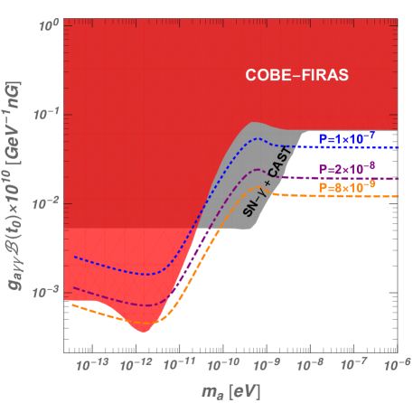
Figure 5: Parameter region of the ALP scenario of Moroi:2018vci excluded by the observational constraints. Dotted curves are the contours for three different values of the conversion probability: $P_{a\rightarrow\gamma}=10^{-7},\,2\times 10^{-8},8\times 10^{-9}.$

Here we revisit the ALP scenario of Moroi:2018vci and update the observational constraints on the model parameters. Our results are summarized in Fig. 5.

The red-colored region in Fig. 5 which was derived in Moroi:2018vci is excluded as it results in a too large distortion of the CMB spectrum probed by the COBE-FIRAS. The gray-colored region is excluded by combining the constraint on $g_{a\gamma\gamma}$ from the absence of $\gamma$-ray burst associated with SN1987A Payez:2014xsa and the recently derived upper bound $B_{0}\lesssim 0.1\,{\rm nG}$ on the primordial magnetic field to avoid an overheating of baryons which would wash away the EDGES signal Minoda:2018gxj . One may consider also the constraint from blackhole supperradiance, which is known to exclude the ALP mass range $7\times 10^{-14}{\rm eV}<m_{a}<2\times 10^{-11}{\rm eV}$ at 95 % confidence level if the ALP quartic coupling is weak enough Stott:2018opm . However this does not apply for the present case as the axion decay constant $f_{a}$ suggested by the size of $g_{a\gamma\gamma}$ implies that the corresponding axion quartic coupling $\lambda\sim m_{a}^{2}/f_{a}^{2}$ is large enough to invalidate the blackhole supperradiance argument.

In Fig. 5, the dotted lines show the parameter region yielding the minimal conversion probability $P_{a\rightarrow\gamma}={\cal O}(10^{-8}-10^{-7})$ which is required to explain the EDGES anomaly. We then find that only a tiny parameter region of $(m_{a},g_{a\gamma\gamma})$ can provide a viable explanation for the EDGES anomaly, but only when both $B_{0}$ and the ALP number density in the 21 cm frequency region nearly saturate their upper bounds.

References

(1)
J. D. Bowman, A. E. E. Rogers, R. A. Monsalve, T. J. Mozdzen and N. Mahesh,
Nature 555, no. 7694, 67 (2018)
doi:10.1038/nature25792
[arXiv:1810.05912 [astro-ph.CO]].
(3)
M. Pospelov, J. Pradler, J. T. Ruderman and A. Urbano,
Phys. Rev. Lett. 121, no. 3, 031103 (2018)
doi:10.1103/PhysRevLett.121.031103
[arXiv:1803.07048 [hep-ph]].
(4)
T. Moroi, K. Nakayama and Y. Tang,
Phys. Lett. B 783, 301 (2018)
doi:10.1016/j.physletb.2018.07.002
[arXiv:1804.10378 [hep-ph]].
(5)
A. Mirizzi, J. Redondo and G. Sigl,
JCAP 0903, 026 (2009)
doi:10.1088/1475-7516/2009/03/026
[arXiv:0901.0014 [hep-ph]].
(6)
A. Mirizzi, J. Redondo and G. Sigl,
JCAP 0908, 001 (2009)
doi:10.1088/1475-7516/2009/08/001
[arXiv:0905.4865 [hep-ph]].
(7)
M. Reece,
JHEP 1907, 181 (2019)
doi:10.1007/JHEP07(2019)181
[arXiv:1808.09966 [hep-th]].
(8)
For a recent rigorous discussion of this issue, see for instance
D. Harlow and H. Ooguri,
arXiv:1810.05338 [hep-th].
(9)
A. Payez, C. Evoli, T. Fischer, M. Giannotti, A. Mirizzi and A. Ringwald,
JCAP 1502, 006 (2015)
doi:10.1088/1475-7516/2015/02/006
[arXiv:1410.3747 [astro-ph.HE]].
(10)
T. Minoda, H. Tashiro and T. Takahashi,
Mon. Not. Roy. Astron. Soc. 488, no. 2, 2001 (2019)
doi:10.1093/mnras/stz1860
[arXiv:1812.00730 [astro-ph.CO]].
(11)
K. Choi, H. Kim and T. Sekiguchi,
Phys. Rev. Lett. 121, no. 3, 031102 (2018)
doi:10.1103/PhysRevLett.121.031102
[arXiv:1802.07269 [hep-ph]].
(12)
K. Choi, H. Kim and S. Yun,
Phys. Rev. D 90, 023545 (2014)
doi:10.1103/PhysRevD.90.023545
[arXiv:1404.6209 [hep-th]].
(13)
K. Choi and S. H. Im,
JHEP 1601, 149 (2016)
doi:10.1007/JHEP01(2016)149
[arXiv:1511.00132 [hep-ph]].
(14)
D. E. Kaplan and R. Rattazzi,
Phys. Rev. D 93, no. 8, 085007 (2016)
doi:10.1103/PhysRevD.93.085007
[arXiv:1511.01827 [hep-ph]].
(15)
T. Higaki, K. S. Jeong, N. Kitajima and F. Takahashi,
Phys. Lett. B 755, 13 (2016)
doi:10.1016/j.physletb.2016.01.055
[arXiv:1512.05295 [hep-ph]].
(16)
M. Farina, D. Pappadopulo, F. Rompineve and A. Tesi,
JHEP 1701, 095 (2017)
doi:10.1007/JHEP01(2017)095
[arXiv:1611.09855 [hep-ph]].
(17)
P. Agrawal, J. Fan, M. Reece and L. T. Wang,
JHEP 1802, 006 (2018)
doi:10.1007/JHEP02(2018)006
[arXiv:1709.06085 [hep-ph]].
(18)
K. Choi, S. Lee, H. Seong and S. Yun,
arXiv:1806.09508 [hep-ph].
(19)
M. Born and E. Wolf, Principles of Optics.
Pergamon Press, 1980.
691-692.
(20)
S. Seager, D. D. Sasselov and D. Scott,
Astrophys. J. 523, L1 (1999)
doi:10.1086/312250
[astro-ph/9909275].
(21)
D. J. Fixsen, E. S. Cheng, J. M. Gales, J. C. Mather, R. A. Shafer and E. L. Wright,
Astrophys. J. 473, 576 (1996)
doi:10.1086/178173
[astro-ph/9605054].
(22)
P. A. R. Ade et al. [Planck Collaboration],
Astron. Astrophys. 594, A13 (2016)
doi:10.1051/0004-6361/201525830
[arXiv:1502.01589 [astro-ph.CO]].
(23)
K. Choi, E. J. Chun and J. E. Kim,
Phys. Lett. B 403, 209 (1997)
doi:10.1016/S0370-2693(97)00465-6
[hep-ph/9608222].
(24)
K. Kaneta, H. S. Lee and S. Yun,
Phys. Rev. Lett. 118, no. 10, 101802 (2017)
doi:10.1103/PhysRevLett.118.101802
[arXiv:1611.01466 [hep-ph]].
(25)
K. Kaneta, H. S. Lee and S. Yun,
Phys. Rev. D 95, no. 11, 115032 (2017)
doi:10.1103/PhysRevD.95.115032
[arXiv:1704.07542 [hep-ph]].
(26)
L. Wolfenstein,
Phys. Rev. D 17 (1978) 2369.
doi:10.1103/PhysRevD.17.2369
(27)
S. P. Mikheyev and A. Y. Smirnov,
Sov. J. Nucl. Phys. 42, 913 (1985)
[Yad. Fiz. 42, 1441 (1985)].
(28)
S. P. Mikheev and A. Y. Smirnov,
Nuovo Cim. C 9, 17 (1986).
doi:10.1007/BF02508049
(29)
S. J. Parke,
Phys. Rev. Lett. 57, 1275 (1986).
doi:10.1103/PhysRevLett.57.1275
(30)
L. D. Landau,
Phys. Z. Sowjetunion, 1, 426 (1932)
(31)
C. Zener,
Proc. Roy. Soc. Lond. A 137, 696 (1932).
doi:10.1098/rspa.1932.0165
(32)
N. Kitajima, T. Sekiguchi and F. Takahashi,
Phys. Lett. B 781, 684 (2018)
doi:10.1016/j.physletb.2018.04.024
[arXiv:1711.06590 [hep-ph]].
(33)
P. Agrawal, N. Kitajima, M. Reece, T. Sekiguchi and F. Takahashi,
arXiv:1810.07188 [hep-ph].
(34)
D. Grin, M. A. Amin, V. Gluscevic, R. Hlǒzek, D. J. E. Marsh, V. Poulin, C. Prescod-Weinstein and T. L. Smith,
arXiv:1904.09003 [astro-ph.CO].
(35)
M. J. Stott and D. J. E. Marsh,
Phys. Rev. D 98, no. 8, 083006 (2018)
doi:10.1103/PhysRevD.98.083006
[arXiv:1805.02016 [hep-ph]].