On some computational aspects of Hermite wavelets on a class of SBVPs arising in exothermic reactions

Amit K. Vermaa, Diksha Tiwarib
aDepartment of Mathematics, IIT Patna, Patna 801106801106801106, Bihar, India.
bFaculty of Mathematics, University of Vienna, Austria.
Email:aakverma@iitp.ac.in,bdikshatiwari227@gmail.com
Abstract

We propose a new class of SBVPs which deals with exothermic reactions. We also propose four computationally stable methods to solve singular nonlinear BVPs by using Hermite wavelet collocation which are coupled with Newton’s quasilinearization and Newton-Raphson method. We compare the results obtained with Hermite Wavelets with Haar wavelet collocation. The efficiency of these methods are verified by applying these four methods on Lane-Emden equations. Convergence analysis is also presented.

Keywords: MRA; Quasilinearization; Newton Raphson; Haar Wavelets; Hermite Wavelets; Nonlinear Singular Boundary value problems,

1 Introduction

This paper deals with Wavelets and nonlinear singular BVPs. Nonlinear BVPs are difficult to deal and if singularity is also present it becomes even more difficult. It is not easy to capture the behavior of the solutions near the point of singularity. If we apply suitable boundary conditions which forces the existence of unique continuous solutions and hence there is possibility of finding these solutions via numerical methods. Still since the coefficient blow up when near the singularity discretizing the differential equation is a challenge. Wavelets help us to treat this complicated situation in an easy way with less number of spatial points. To address both nonlinear BVPs and Wavelets we divide the introduction in two parts.

Nonlinear SBVPs arising in Exothermic Reactions

Here we propose a new class of nonlinear SBVP. For that let us consider the mathematical equation which governs, balance between heat generated and conducted away

λ2T=QW,𝜆superscript2𝑇𝑄𝑊\lambda\nabla^{2}T=-QW, (1)

where T𝑇T is gas temperature, Q𝑄Q the heat of the reaction, λ𝜆\lambda the thermal conductivity, W𝑊W the reaction velocity and 2superscript2\nabla^{2} the Laplacian operator.

Chambre [4] assumed that reaction is mono-molecular and velocity follows the Arrhenius law, given as

W=Aexp(ERT),𝑊𝐴𝐸𝑅𝑇W=A\exp\left(\frac{-E}{RT}\right), (2)

and after some approximations and symmetry assumptions Chambre [4] arrived at the following equation

Ly=δexp(t)𝐿𝑦𝛿𝑡Ly=-\delta\exp(t) (3)

where,

Ld2dt2+kgtddt,𝐿superscript𝑑2𝑑superscript𝑡2subscript𝑘𝑔𝑡𝑑𝑑𝑡L\equiv\frac{d^{2}}{dt^{2}}+\frac{k_{g}}{t}\frac{d}{dt},

kgsubscript𝑘𝑔k_{g} depends on shape and size of the vessel and δ𝛿\delta is a parameter.

Nakamura et al. [15], while looking for an equation which can express the temperature dependence of the rate constant proposed the following

W=Aexp(ER(T0n+Tn)1/n),n=1,2,3,formulae-sequence𝑊𝐴𝐸𝑅superscriptsuperscriptsubscript𝑇0𝑛superscript𝑇𝑛1𝑛𝑛123W=A\exp\left(\frac{-E}{R~{}\left(T_{0}^{n}+T^{n}\right)^{1/n}}\right),\quad n=1,2,3,\cdots (4)

where R𝑅R is a gas constant, T𝑇T is absolute temperature, A𝐴A, E0subscript𝐸0E_{0} and T0subscript𝑇0T_{0} are parameters and n𝑛n is an integer.

Similar to analysis of Chambre [4], we arrive at the following differential equation

Ly=Bexp(A(cn+yn)1/n).𝐿𝑦𝐵𝐴superscriptsuperscript𝑐𝑛superscript𝑦𝑛1𝑛Ly=-B\exp\left(\frac{-A}{\left(c^{n}+y^{n}\right)^{1/n}}\right). (5)

There are several other examples which led us to consider the following class of nonlinear singular boundary value problem (SBVPs)

Ly+f(t,y(t))=0,0<t1,formulae-sequence𝐿𝑦𝑓𝑡𝑦𝑡00𝑡1Ly+{f(t,y(t))}=0,\quad\quad\quad 0<t\leq 1, (6)

subject to following the boundary conditions

Case(i)y(0)=α,y(1)=β,formulae-sequence𝐶𝑎𝑠𝑒𝑖superscript𝑦0𝛼𝑦1𝛽\displaystyle Case~{}(i)\quad~{}~{}y^{\prime}(0)=\alpha,\quad y(1)=\beta, (7a)
Case(ii)y(0)=α,y(1)=β,formulae-sequence𝐶𝑎𝑠𝑒𝑖𝑖𝑦0𝛼𝑦1𝛽\displaystyle Case~{}(ii)\quad~{}y(0)=\alpha,\quad y(1)=\beta, (7b)
Case(iii)y(0)=α,ay(1)+by(1)=β,formulae-sequence𝐶𝑎𝑠𝑒𝑖𝑖𝑖superscript𝑦0𝛼𝑎𝑦1𝑏superscript𝑦1𝛽\displaystyle Case~{}(iii)\quad y^{\prime}(0)=\alpha,\quad ay(1)+by^{\prime}(1)=\beta, (7c)

where a,b,c𝑎𝑏𝑐a,b,c, α𝛼\alpha, β𝛽\beta are real constants and f(t,y(t))𝑓𝑡𝑦𝑡{f\left(t,y(t)\right)} is a real valued function. Boundary conditions at the singular end t=0𝑡0t=0 depend on the value of kgsubscript𝑘𝑔k_{g}.

There is huge literature on existence of solutions of such BVPs. Please refer [17], [18], [19] and [28] and the references there in. Several numerical methods have also been proposed for solving these type of non-linear singular boundary value problems (see [25, 24, 30] and its references).

In [10] non linear singular Lane-Emden IVPs are solved with Haar Wavelet Quasilinearization approach, and nonlinearity is easily handled with quasilinearization. In [22] Hermite wavelets operational matrix method is used to solve second order nonlinear singular initial value problems. In [16] Chebyshev wavelets operation matrices are used for solving nonlinear singular boundary value problems. In [31] method based on Laguerre wavelets is used to solve nonlinear singular boundary value problems. In [14] method based on Legendre wavelet is proposed to solve singular boundary value problems. All these based on wavelets show high accuracy. In [29, 27, 26] Haar wavelets are used to solve SBVPs efficiently for higher resolution.

In this article we solve SBVP of type (6) subject to boundary conditions (7a),(7b),(7c) with help of Hermite Wavelet Newton Approach (HeWNA), Hermite Wavelet Quasilinearization Approach (HeWQA), Haar wavelet Newton Approach (HWNA) and Haar Wavelet Quasilinearization Approach (HWQA) and compare results to show accuracy of the method. Convergence of HeWNA method is also established. Novelty of this paper is that Newton Raphson has not been coupled with Haar wavelets and Hermite has not been used to solve Nonlinear Singular BVPs till now.

Some recent works on wavelets and their applications can be find in [9, 2, 23, 11] and the references there in.

This paper is organized in the following manner. In section 2 we discuss MRA and Hermite wavelet is defined, in sub section 2.3 Haar wavelet is defined, in section 3 method of solution based on HeWQA, HeWNA, HWQA and HWNA are proposed. In section 4, convergence analysis of HWNA method is done and in the last section some numerical examples are presented to show accuracy of the method.

2 Hermite and Haar Wavelet

This section starts with MRA and definition of Hermite Wavelets.

2.1 Wavelets and MRA

The theory of Wavelets are developed by mathematicians as well engineers over the years. Wavelet word find its origin the name of French geophysicist Jean Morlet (1931–2007). He used wavelet to describe certain functions. Morlet and Croatian-French physicist Alex Grossman developed theory further which is used now a days [20, p. 222]. Main issue that was being addressed in the process, was to overcome drawbacks of Fourier transforms. Wavelets are multi-indexed and it contains parameters which can be used to shift or dilate/contract the functions giving us basis functions. Thus computationally they are complex but they have better control and much better results are obtained at low resolution, i.e., less number of divisions are needed that we need in finite difference and all methods based on similar concepts. Here we consider methods based on wavelet transforms.

The following properties of wavelets enable us to choose them over other methods:

  • Orthogonality

  • Compact Support

  • Density

  • Multiresolution Analysis (MRA)

2.1.1 MRA

Pereyra et al. [20] observe that an orthogonal multiresolution analysis (MRA) is a collection of closed subspaces of L2()superscript𝐿2L^{2}(\mathbb{R}) which are nested, having trivial intersection, they exhaust the space, the subspaces are connected to each other by scaling property and finally there is a special function, the scaling function φ𝜑\varphi, whose integer translates form an orthonormal basis for one of the subspaces. We give formal statement of MRA as defined in [20].

Definition 2.1.

An MRA with scaling function φ𝜑\varphi is a collection of closed subspaces Vj,j=,2,1,0,1,2,formulae-sequencesubscript𝑉𝑗𝑗21012italic-…V_{j},j=\dots,—2,—1,0,1,2,\dots of L2()superscript𝐿2L^{2}(\mathbb{R}) such that

  1. 1.

    𝐕j𝐕j+1subscript𝐕𝑗subscript𝐕𝑗1\mathbf{V}_{j}\subset\mathbf{V}_{j+1}

  2. 2.

    𝐕j¯=𝐋𝟐()¯subscript𝐕𝑗superscript𝐋2\overline{\bigcup\mathbf{V}_{j}}=\mathbf{L^{2}(\mathbb{R})}

  3. 3.

    𝐕j=0subscript𝐕𝑗0\bigcap\mathbf{V}_{j}={0}

  4. 4.

    The function f(x)𝑓𝑥f(x) belongs to 𝐕jsubscript𝐕𝑗\mathbf{V}_{j} if and only if the function f(2x)𝐕j+1𝑓2𝑥subscript𝐕𝑗1f(2x)\in\mathbf{V}_{j+1}.

  5. 5.

    The function φ𝜑\varphi belongs to 𝐕0subscript𝐕0\mathbf{V}_{0}, the set {φ(xk),k}𝜑𝑥𝑘𝑘\{\varphi(x-k),k\in\mathbf{\mathbb{Z}}\} is orthonormal basis for 𝐕0subscript𝐕0\mathbf{V}_{0}.

The sequence of wavelet subspaces Wjsubscript𝑊𝑗W_{j} of L2()superscript𝐿2L^{2}(\mathbb{R}), are such that VjWjperpendicular-tosubscript𝑉𝑗𝑊𝑗V_{j}\perp Wj , for all j𝑗j and Vj+1=VjWjsubscript𝑉𝑗1direct-sumsubscript𝑉𝑗subscript𝑊𝑗V_{j+1}=V_{j}\oplus W_{j}. Closure of jWjsubscriptdirect-sum𝑗subscript𝑊𝑗\oplus_{j\in\mathbb{Z}}W_{j} is dense in L2()superscript𝐿2L^{2}(\mathbb{R}) with respect to L2superscript𝐿2L^{2} norm.

Now we state Mallat’s theorem [13] which guarantees that in presence of an orthogonal MRA, an orthonormal basis for L2()superscript𝐿2L^{2}(\mathbb{R}) exists. These basis functions are fundamental functions in the theory of wavelets which helps us to develop advanced computational techniques.

Theorem 2.1.

(MallatsTheorem)superscriptMallatsTheorem\mathrm{(Mallat^{\prime}s~{}Theorem)}. Given an orthogonal MRA with scaling function φ𝜑\varphi, there is a wavelet ψL2()𝜓superscript𝐿2\psi\in L^{2}(\mathbb{R}) such that for each j𝑗j\in\mathbb{Z}, the family {ψj,k}ksubscriptsubscript𝜓𝑗𝑘𝑘\{\psi_{j,k}\}_{k\in\mathbb{Z}} is an orthonormal basis for Wjsubscript𝑊𝑗W_{j} . Hence the family {ψj,k}ksubscriptsubscript𝜓𝑗𝑘𝑘\{\psi_{j,k}\}_{k\in\mathbb{Z}} is an orthonormal basis for L2()superscript𝐿2L^{2}(\mathbb{R}).

2.2 Hermite Wavelet ([21])

Hermite Polynomials are defined on the interval (,)(-\infty,\infty) and can be defined with help of the recurrence formula:

H0(t)=1subscript𝐻0𝑡1\displaystyle H_{0}(t)=1
H1(t)=2tsubscript𝐻1𝑡2𝑡\displaystyle H_{1}(t)=2t
Hm+1(t)=2tHm(t)2mHm1(t),m=1,2,3,.formulae-sequencesubscript𝐻𝑚1𝑡2𝑡subscript𝐻𝑚𝑡2𝑚subscript𝐻𝑚1𝑡𝑚123\displaystyle H_{m+1}(t)=2tH_{m}(t)-2mH_{m-1}(t),~{}m=1,2,3,\cdots.

Completeness and orthogonality (with respect to weight function et2superscript𝑒superscript𝑡2e^{-t^{2}}) of Hermite polynomials enable us to treat them as wavelet (Theorem 2.1).

Hermite wavelet on the interval [0,1]01[0,1] are defined as

ψn,m(t)=2k/21n!2nπHm(2ktn^)χ[n^12k,n^+12k)subscript𝜓𝑛𝑚𝑡superscript2𝑘21𝑛superscript2𝑛𝜋subscript𝐻𝑚superscript2𝑘𝑡^𝑛subscript𝜒^𝑛1superscript2𝑘^𝑛1superscript2𝑘\psi_{n,m}(t)=2^{k/2}\frac{1}{\sqrt{n!2^{n}\sqrt{\pi}}}H_{m}(2^{k}t-\hat{n})\chi_{\left[\frac{\hat{n}-1}{2^{k}},\frac{\hat{n}+1}{2^{k}}\right)} (8)

where k=1,2,𝑘12k=1,2,\ldots is level of resolution, n=1,2,,2k1,n^=2n1formulae-sequence𝑛12superscript2𝑘1^𝑛2𝑛1n=1,2,\ldots,2^{k-1},\hskip 7.11317pt\hat{n}=2n-1 is translation parameter, m=1,2,,M1𝑚12𝑀1m=1,2,\ldots,M-1 is order of Hermite polynomial.

2.2.1 Approximation of Function with Hermite Wavelet

A function f(t)𝑓𝑡f(t) defined on L2[0,1]superscript𝐿201L^{2}[0,1] can be approximated with Hermite wavelet in the following manner

f(t)=n=1m=0cnmψnm(t).𝑓𝑡subscriptsuperscript𝑛1subscriptsuperscript𝑚0subscript𝑐𝑛𝑚subscript𝜓𝑛𝑚𝑡f(t)=\sum^{\infty}_{n=1}\sum^{\infty}_{m=0}c_{nm}\psi_{nm}(t). (9)

For computation purpose we truncate (9) and define,

f(t)n=12k1m=0M1cnmψnm(t)=cTψ(t)similar-to-or-equals𝑓𝑡subscriptsuperscriptsuperscript2𝑘1𝑛1subscriptsuperscript𝑀1𝑚0subscript𝑐𝑛𝑚subscript𝜓𝑛𝑚𝑡superscript𝑐𝑇𝜓𝑡f(t)\simeq\sum^{2^{k}-1}_{n=1}\sum^{M-1}_{m=0}c_{nm}\psi_{nm}(t)=c^{T}\psi(t) (10)

where ψ(t)𝜓𝑡\psi(t) is 2k1M×1superscript2𝑘1𝑀12^{k-1}M\times 1 matrix given as:

ψ(t)=[ψ1,0(t),,ψ1,M1(t),ψ2,0(t),,ψ2,M1(t),,ψ2k1,0(t),,ψ2k1,M1(t)]T𝜓𝑡superscriptsubscript𝜓10𝑡subscript𝜓1𝑀1𝑡subscript𝜓20𝑡subscript𝜓2𝑀1𝑡subscript𝜓superscript2𝑘10𝑡subscript𝜓superscript2𝑘1𝑀1𝑡𝑇\psi(t)=\left[\psi_{1,0}(t),\dots,\psi_{1,M-1}(t),\psi_{2,0}(t),\dots,\psi_{2,M-1}(t),\dots,\psi_{2^{k-1},0}(t),\dots,\psi_{2^{k-1},M-1}(t)\right]^{T}

c𝑐c is 2k1M×1superscript2𝑘1𝑀12^{k-1}M\times 1 matrix. Entries of c𝑐c can be computed as

cij=01f(t)ψij(t)𝑑tsubscript𝑐𝑖𝑗subscriptsuperscript10𝑓𝑡subscript𝜓𝑖𝑗𝑡differential-d𝑡c_{ij}=\int^{1}_{0}f(t)\psi_{ij}(t)dt (11)

with i=1,2,,2k1𝑖12superscript2𝑘1i=1,2,\dots,2^{k}-1 and j=0,1,,M1𝑗01𝑀1j=0,1,\dots,M-1. Here M𝑀M is degree of Hermite polynomial.

2.2.2 Integration of Hermite Wavelet

As suggested in [1], ν𝜈\nu-th order integration of ψ(t)𝜓𝑡\psi(t) can also be approximated as

0t0t0tψ(τ)𝑑τ[Jνψ1,0(t),,Jνψ1,M1(t),Jνψ2,0(t),,Jνψ2,M1(t),,Jνψ2k1,0(t),,Jνψ2k1,M1(t)]Tsimilar-to-or-equalssubscriptsuperscript𝑡0subscriptsuperscript𝑡0subscriptsuperscript𝑡0𝜓𝜏differential-d𝜏superscriptsuperscript𝐽𝜈subscript𝜓10𝑡superscript𝐽𝜈subscript𝜓1𝑀1𝑡superscript𝐽𝜈subscript𝜓20𝑡superscript𝐽𝜈subscript𝜓2𝑀1𝑡superscript𝐽𝜈subscript𝜓superscript2𝑘10𝑡superscript𝐽𝜈subscript𝜓superscript2𝑘1𝑀1𝑡𝑇\int^{t}_{0}\int^{t}_{0}\dots\int^{t}_{0}\psi(\tau)d\tau\simeq\\ \left[J^{\nu}\psi_{1,0}(t),\dots,J^{\nu}\psi_{1,M-1}(t),J^{\nu}\psi_{2,0}(t),\dots,J^{\nu}\psi_{2,M-1}(t),\dots,J^{\nu}\psi_{2^{k-1},0}(t),\dots,J^{\nu}\psi_{2^{k-1},M-1}(t)\right]^{T}

where

Jνψn,m(t)=2k/21n!2nπJνHm(2ktn^)χ[n^12k,n^+12k),superscript𝐽𝜈subscript𝜓𝑛𝑚𝑡superscript2𝑘21𝑛superscript2𝑛𝜋superscript𝐽𝜈subscript𝐻𝑚superscript2𝑘𝑡^𝑛subscript𝜒^𝑛1superscript2𝑘^𝑛1superscript2𝑘J^{\nu}\psi_{n,m}(t)=2^{k/2}\frac{1}{\sqrt{n!2^{n}\sqrt{\pi}}}J^{\nu}H_{m}(2^{k}t-\hat{n})\chi_{\left[\frac{\hat{n}-1}{2^{k}},\frac{\hat{n}+1}{2^{k}}\right)}, (12)

where k=1,2,𝑘12k=1,2,\ldots is level of resolution, n=1,2,,2k1,n^=2n1formulae-sequence𝑛12superscript2𝑘1^𝑛2𝑛1n=1,2,\ldots,2^{k-1},\hskip 7.11317pt\hat{n}=2n-1 is translation parameter, m=1,2,,M1𝑚12𝑀1m=1,2,\ldots,M-1 is order of Hermite polynomial.

Remark 2.1.

Integral operator Jν(ν>0)superscript𝐽𝜈𝜈0J^{\nu}(\nu>0) of a function f(t)𝑓𝑡f(t) is defined as

Jνf(t)=1ν!0t(ts)ν1f(s)𝑑s.superscript𝐽𝜈𝑓𝑡1𝜈superscriptsubscript0𝑡superscript𝑡𝑠𝜈1𝑓𝑠differential-d𝑠J^{\nu}f(t)=\frac{1}{\nu!}\int_{0}^{t}(t-s)^{\nu-1}f(s)ds.

2.2.3 Hermite Wavelet Collocation Method

To apply Hermite wavelet on the ordinary differential equations, we need its discretized form. We use collocation method for discretization where mesh points are given by

x¯l=lΔx,l=0,1,,M1.formulae-sequencesubscript¯𝑥𝑙𝑙Δ𝑥𝑙01𝑀1\displaystyle\bar{x}_{l}=l\Delta x,\quad\quad\quad l=0,1,\cdots,M-1. (13)

For the collocation points we define

xl=0.5(x¯l1+x¯l),l=0,1,,M1.formulae-sequencesubscript𝑥𝑙0.5subscript¯𝑥𝑙1subscript¯𝑥𝑙𝑙01𝑀1\displaystyle x_{l}=0.5(\bar{x}_{l-1}+\bar{x}_{l}),\quad\quad\quad l=0,1,\cdots,M-1. (14)

For k=1𝑘1k=1, equation (10) takes the form

f(t)m=0M1c1mψ1m(t).similar-to-or-equals𝑓𝑡subscriptsuperscript𝑀1𝑚0subscript𝑐1𝑚subscript𝜓1𝑚𝑡f(t)\simeq\sum^{M-1}_{m=0}c_{1m}\psi_{1m}(t). (15)

We replace t𝑡t by xlsubscript𝑥𝑙x_{l} in above equation and arrive at system of equations which can easily be solved to get the solution of the nonlinear SBVP.

2.3 Haar Wavelet

Let us assume that x𝑥x belongs to any interval [P,Q]𝑃𝑄[P,Q], where P𝑃P and Q𝑄Q are constant end points. Let us define M=2J𝑀superscript2𝐽M=2^{J}, where J𝐽J is the maximal level of resolution. Devide [P,Q]𝑃𝑄[P,Q] into 2M2𝑀2M subintervals of equal length Δx=(QP)/(2M)Δ𝑥𝑄𝑃2𝑀\Delta x=(Q-P)/(2M). The wavelet number i𝑖i is defined as i=m+k+1𝑖𝑚𝑘1i=m+k+1, where j=0,1,,J𝑗01𝐽j=0,1,\cdots,J and k=0,1,,m1𝑘01𝑚1k=0,1,\cdots,m-1 (here m=2j𝑚2𝑗m=2j). The ithsuperscript𝑖𝑡i^{th} Haar wavelet is explained as

hi(x)=χ[η1(i),η2(i))χ[η2(i),η3(i))subscript𝑖𝑥subscript𝜒subscript𝜂1𝑖subscript𝜂2𝑖subscript𝜒subscript𝜂2𝑖subscript𝜂3𝑖h_{i}(x)=\chi_{\left[{\eta}_{1}\left(i\right),{\eta}_{2}\left(i\right)\right)}-\chi_{\left[{\eta}_{2}\left(i\right),{\eta}_{3}\left(i\right)\right)} (16)

where

η1(i)=P+2kμΔx,η2(i)=P+(2k+1)μΔx,η3(i)=P+2(k+1)μΔx,μ=M/m.formulae-sequencesubscript𝜂1𝑖𝑃2𝑘𝜇Δ𝑥formulae-sequencesubscript𝜂2𝑖𝑃2𝑘1𝜇Δ𝑥formulae-sequencesubscript𝜂3𝑖𝑃2𝑘1𝜇Δ𝑥𝜇𝑀𝑚\displaystyle\eta_{1}(i)=P+2k\mu\Delta x,\quad\eta_{2}(i)=P+(2k+1)\mu\Delta x,\quad\eta_{3}(i)=P+2(k+1)\mu\Delta x,\quad\mu=M/m. (17)

Above equations are valid for i>2𝑖2i>2. For i=1𝑖1i=1 case we have, hi(x)=χ[P,Q]subscript𝑖𝑥subscript𝜒𝑃𝑄h_{i}(x)=\chi_{[P,Q]}.

For i=2𝑖2i=2 we have

η1(2)=P,η2(2)=0.5(2P+Q),η3(2)=Q.formulae-sequencesubscript𝜂12𝑃formulae-sequencesubscript𝜂220.52𝑃𝑄subscript𝜂32𝑄\displaystyle\eta_{1}(2)=P,\quad\eta_{2}(2)=0.5(2P+Q),\quad\eta_{3}(2)=Q. (18)

The thickness of the ithsuperscript𝑖𝑡i^{th} wavelet is

η3(i)η1(i)=2μΔx=(QP)m1=(QP)2j.subscript𝜂3𝑖subscript𝜂1𝑖2𝜇Δ𝑥𝑄𝑃superscript𝑚1𝑄𝑃superscript2𝑗\displaystyle\eta_{3}(i)-\eta_{1}(i)=2\mu\Delta x=(Q-P)m^{-1}=(Q-P)2^{-j}. (19)

If J𝐽J is fixed then by (16)

PQhi(x)hl(x)𝑑x={(QP)2j,l=i,0,li.superscriptsubscript𝑃𝑄subscript𝑖𝑥subscript𝑙𝑥differential-d𝑥cases𝑄𝑃superscript2𝑗𝑙𝑖0𝑙𝑖\displaystyle\int_{P}^{Q}h_{i}(x)h_{l}(x)dx=\begin{cases}(Q-P)2^{-j},&l=i,\\ 0,&l\neq i.\end{cases} (20)

The integrals pυ,i(x)subscript𝑝𝜐𝑖𝑥p_{\upsilon,i}(x) are defined as

pυ,i(x)=PxPxPxhi(t)𝑑tv=1(v1)!Px(xt)(υ1)hi(t)𝑑t,subscript𝑝𝜐𝑖𝑥superscriptsubscript𝑃𝑥superscriptsubscript𝑃𝑥superscriptsubscript𝑃𝑥subscript𝑖𝑡differential-dsuperscript𝑡𝑣1𝑣1superscriptsubscript𝑃𝑥superscript𝑥𝑡𝜐1subscript𝑖𝑡differential-d𝑡\displaystyle p_{\upsilon,i}(x)=\int_{P}^{x}\int_{P}^{x}\cdots\int_{P}^{x}h_{i}(t)dt^{v}=\frac{1}{(v-1)!}\int_{P}^{x}(x-t)^{(\upsilon-1)}h_{i}(t)dt, (21)

where υ=1,2,,n,i=1,2,,2M.formulae-sequence𝜐12𝑛𝑖122𝑀\upsilon=1,2,\cdots,n,\quad i=1,2,\cdots,2M.

Putting all values in the integral we get

pυ,i(x)=1υ![xη1(i)]υχ[η1(i),η2(i))+1υ!{[xη1(i)]υ2[xη2(i)]υ}χ[η2(i),η3(i)]+1υ!{[xη1(i)]υ2[xη2(i)]υ+[xη3(i)]υ}χ(η3(i),)subscript𝑝𝜐𝑖𝑥1𝜐superscriptdelimited-[]𝑥subscript𝜂1𝑖𝜐subscript𝜒subscript𝜂1𝑖subscript𝜂2𝑖1𝜐superscriptdelimited-[]𝑥subscript𝜂1𝑖𝜐2superscriptdelimited-[]𝑥subscript𝜂2𝑖𝜐subscript𝜒subscript𝜂2𝑖subscript𝜂3𝑖1𝜐superscriptdelimited-[]𝑥subscript𝜂1𝑖𝜐2superscriptdelimited-[]𝑥subscript𝜂2𝑖𝜐superscriptdelimited-[]𝑥subscript𝜂3𝑖𝜐subscript𝜒subscript𝜂3𝑖p_{\upsilon,i}(x)=\frac{1}{\upsilon!}[x-\eta_{1}(i)]^{\upsilon}\chi_{\left[{\eta}_{1}\left(i\right),{\eta}_{2}\left(i\right)\right)}+\frac{1}{\upsilon!}\{[x-\eta_{1}(i)]^{\upsilon}-2[x-\eta_{2}(i)]^{\upsilon}\}\chi_{\left[{\eta}_{2}\left(i\right),{\eta}_{3}\left(i\right)\right]}\\ +\frac{1}{\upsilon!}\{[x-\eta_{1}(i)]^{\upsilon}-2[x-\eta_{2}(i)]^{\upsilon}+[x-\eta_{3}(i)]^{\upsilon}\}\chi_{(\eta_{3}(i),\infty)} (22)

for i>1𝑖1i>1 and for i=1𝑖1i=1 we have η1=P,η2=η3=Qformulae-sequencesubscript𝜂1𝑃subscript𝜂2subscript𝜂3𝑄\eta_{1}=P,\eta_{2}=\eta_{3}=Q and

pυ,1(x)=1υ!(xP)υ.subscript𝑝𝜐1𝑥1𝜐superscript𝑥𝑃𝜐p_{\upsilon,1}(x)=\frac{1}{\upsilon!}(x-P)^{\upsilon}. (23)

2.3.1 Haar Wavelet Collocation Method

Similar to case of previous section here again we define collocation points as follows

x¯t=P+tΔx,t=0,1,,2M,formulae-sequencesubscript¯𝑥𝑡𝑃𝑡Δ𝑥𝑡012𝑀\displaystyle\bar{x}_{t}=P+t\Delta x,\quad\quad\quad~{}t=0,1,\cdots,2M, (24)
xt=0.5(x¯t1+x¯t),t=0,1,,2M,formulae-sequencesubscript𝑥𝑡0.5subscript¯𝑥𝑡1subscript¯𝑥𝑡𝑡012𝑀\displaystyle x_{t}=0.5(\bar{x}_{t-1}+\bar{x}_{t}),\quad t=0,1,\cdots,2M, (25)

and replace xxt𝑥subscript𝑥𝑡x\to x_{t} in (16),(17),(18). We define the Haar matrices H,P1,P2,,Pυ𝐻subscript𝑃1subscript𝑃2subscript𝑃𝜐H,P_{1},P_{2},\cdots,P_{\upsilon} which are 2M×2M2𝑀2𝑀2M\times 2M matrices. Entries of matrices are given by H(i,t)=hi(xt)𝐻𝑖𝑡subscript𝑖subscript𝑥𝑡H(i,t)=h_{i}(x_{t}), Pv(i,t)=Pυ,i(xt)subscript𝑃𝑣𝑖𝑡subscript𝑃𝜐𝑖subscript𝑥𝑡P_{v}(i,t)=P_{\upsilon,i}(x_{t}), υ=1,2,𝜐12\upsilon=1,2,\cdots. Consider P=0,Q=1,J=1formulae-sequence𝑃0formulae-sequence𝑄1𝐽1P=0,Q=1,J=1. Then 2M=42𝑀42M=4, so H,P1,P2𝐻subscript𝑃1subscript𝑃2H,P_{1},P_{2} are defined as

H=[1111111111000011],P1=18[1357133111000011],P2=1128[19254919233117880017].formulae-sequence𝐻delimited-[]1111111111000011formulae-sequencesubscript𝑃118delimited-[]1357133111000011subscript𝑃21128delimited-[]19254919233117880017\displaystyle H=\left[\begin{array}[]{cccc}1&1&1&1\\ 1&1&-1&-1\\ 1&-1&0&0\\ 0&0&1&-1\end{array}\right],\quad P_{1}=\frac{1}{8}\left[\begin{array}[]{cccc}1&3&5&7\\ 1&3&3&1\\ 1&1&0&0\\ 0&0&1&1\end{array}\right],\quad P_{2}=\frac{1}{128}\left[\begin{array}[]{cccc}1&9&25&49\\ 1&9&23&31\\ 1&7&8&8\\ 0&0&1&7\end{array}\right]. (38)

2.3.2 Approximation of Function with Haar Wavelet

A function f(t)𝑓𝑡f(t) defined on L2[0,1]superscript𝐿201L^{2}[0,1] can be approximated by Haar wavelet basis in the following manner

f(t)=i=0aihi(t).𝑓𝑡subscriptsuperscript𝑖0subscript𝑎𝑖subscript𝑖𝑡f(t)=\sum^{\infty}_{i=0}a_{i}h_{i}(t). (39)

For computation purpose we truncate (39) and define

f(t)i=02Maihi(t),similar-to-or-equals𝑓𝑡subscriptsuperscript2𝑀𝑖0subscript𝑎𝑖subscript𝑖𝑡f(t)\simeq\sum^{2M}_{i=0}a_{i}h_{i}(t), (40)

where M𝑀M is level of resolution.

3 Numerical Methods Based on Hermite and Haar Wavelets

In this section, solution methods based on Hermite wavelet and Haar wavelet are presented.

3.1 Hermite Wavelet Quasilinearization Approach (HeWQA)

In HeWQA we use quasilinearization to linearize SBVP then method of collocation for discretization and use Hermite wavelets for computation of solutions to nonlinear SBVP. We consider differential equation (6) with boundary conditions (7a), (7b) and (7c). Quasilinearizing this equation, we get the form

Lyr+1=f(t,yr(t))+s=01(yr+1syrs)(fys(t,yr(t)),\displaystyle Ly_{r+1}=-f(t,y_{r}(t))+\sum_{s=0}^{1}(y_{r+1}^{s}-y_{r}^{s})(-f_{y^{s}}(t,y_{r}(t)), (41a)
subject to linearized boundary conditions,
yr+1(0)=yr(0),yr+1(1)=yr(1),formulae-sequencesubscriptsuperscript𝑦𝑟10subscript𝑦𝑟0subscript𝑦𝑟11subscript𝑦𝑟1\displaystyle y^{\prime}_{r+1}(0)=y_{r}(0),\quad{y_{r+1}(1)}={y_{r}(1)}, (41b)
yr+1(0)=yr(0),yr+1(1)=yr(1),formulae-sequencesubscript𝑦𝑟10subscript𝑦𝑟0subscript𝑦𝑟11subscript𝑦𝑟1\displaystyle y_{r+1}(0)=y_{r}(0),\quad{y_{r+1}(1)}={y_{r}(1)}, (41c)
yr+1(0)=yr(0),ayr+1(1)+byr+1(1)=ayr(1)+byr(1).formulae-sequencesubscriptsuperscript𝑦𝑟10subscript𝑦𝑟0𝑎subscript𝑦𝑟11𝑏subscriptsuperscript𝑦𝑟11𝑎subscript𝑦𝑟1𝑏subscriptsuperscript𝑦𝑟1\displaystyle y^{\prime}_{r+1}(0)=y_{r}(0),\quad a{y_{r+1}(1)}+by^{\prime}_{r+1}(1)=a{y_{r}(1)}+by^{\prime}_{r}(1). (41d)
Here s=0,1𝑠01s=0,1, fys=f/yssubscript𝑓superscript𝑦𝑠𝑓superscript𝑦𝑠f_{y^{s}}=\partial{f}/\partial{y^{s}} and yr0(t)=yr(t)superscriptsubscript𝑦𝑟0𝑡subscript𝑦𝑟𝑡y_{r}^{0}(t)=y_{r}(t).

Thus we arrive at linearized form of given differential equation. Now we use Hermite wavelet method similar to described in [6]. Let us assume

yr+1′′(t)=m=0M1c1mψ1m(t).subscriptsuperscript𝑦′′𝑟1𝑡subscriptsuperscript𝑀1𝑚0subscript𝑐1𝑚subscript𝜓1𝑚𝑡\displaystyle y^{\prime\prime}_{r+1}(t)=\sum^{M-1}_{m=0}c_{1m}\psi_{1m}(t). (41e)

Then integrating twice we get the following two equations:

yr+1(t)=m=0M1c1mJψ1m(t)+yr+1(0),subscriptsuperscript𝑦𝑟1𝑡subscriptsuperscript𝑀1𝑚0subscript𝑐1𝑚𝐽subscript𝜓1𝑚𝑡subscriptsuperscript𝑦𝑟10\displaystyle y^{\prime}_{r+1}(t)=\sum^{M-1}_{m=0}c_{1m}J\psi_{1m}(t)+y^{\prime}_{r+1}(0), (41f)
yr+1(t)=m=0M1c1mJ2ψ1m(t)+tyr+1(0)+yr+1(0).subscript𝑦𝑟1𝑡subscriptsuperscript𝑀1𝑚0subscript𝑐1𝑚superscript𝐽2subscript𝜓1𝑚𝑡𝑡subscriptsuperscript𝑦𝑟10subscript𝑦𝑟10\displaystyle y_{r+1}(t)=\sum^{M-1}_{m=0}c_{1m}J^{2}\psi_{1m}(t)+ty^{\prime}_{r+1}(0)+y_{r+1}(0). (41g)

Here Jν(ν>0)superscript𝐽𝜈𝜈0J^{\nu}(\nu>0) is the integral operator defined previously.

3.1.1 Treatement of the Boundary Value Problem

Based on boundary conditions we will consider different cases and follow procedure similar to described in [12]. Case (i): In equation (7a) we have y(0)=α,y(1)=βformulae-sequencesuperscript𝑦0𝛼𝑦1𝛽y^{\prime}(0)=\alpha,y(1)=\beta. So by linearization we have yr+1(0)=α,yr+1(1)=βformulae-sequencesubscriptsuperscript𝑦𝑟10𝛼subscript𝑦𝑟11𝛽y^{\prime}_{r+1}(0)=\alpha,y_{r+1}(1)=\beta. Now put t=1𝑡1t=1 in (41g) we get

yr+1(1)=m=0M1c1mJ2ψ1m(1)+yr+1(0)+yr+1(0),subscript𝑦𝑟11subscriptsuperscript𝑀1𝑚0subscript𝑐1𝑚superscript𝐽2subscript𝜓1𝑚1subscriptsuperscript𝑦𝑟10subscript𝑦𝑟10y_{r+1}(1)=\sum^{M-1}_{m=0}c_{1m}J^{2}\psi_{1m}(1)+y^{\prime}_{r+1}(0)+y_{r+1}(0),

so

yr+1(0)=yr+1(1)m=0M1c1mJ2ψ1m(1)yr+1(0).subscript𝑦𝑟10subscript𝑦𝑟11subscriptsuperscript𝑀1𝑚0subscript𝑐1𝑚superscript𝐽2subscript𝜓1𝑚1subscriptsuperscript𝑦𝑟10y_{r+1}(0)=y_{r+1}(1)-\sum^{M-1}_{m=0}c_{1m}J^{2}\psi_{1m}(1)-y^{\prime}_{r+1}(0). (42)

By using equation (42) in (41g) and simplifying we get

yr+1(t)=(t1)yr+1(0)+yr+1(1)+m=0M1c1m(J2ψ1m(t)J2ψ1m(1)).subscript𝑦𝑟1𝑡𝑡1subscriptsuperscript𝑦𝑟10subscript𝑦𝑟11subscriptsuperscript𝑀1𝑚0subscript𝑐1𝑚superscript𝐽2subscript𝜓1𝑚𝑡superscript𝐽2subscript𝜓1𝑚1y_{r+1}(t)=(t-1)y^{\prime}_{r+1}(0)+y_{r+1}(1)+\sum^{M-1}_{m=0}c_{1m}(J^{2}\psi_{1m}(t)-J^{2}\psi_{1m}(1)). (43)

Now putting values of yr+1(0)subscriptsuperscript𝑦𝑟10y^{\prime}_{r+1}(0) and yr+1(1)subscript𝑦𝑟11y_{r+1}(1) in (41f) and (43) we get

yr+1(t)=α+m=0M1c1mJψ1m(t),subscriptsuperscript𝑦𝑟1𝑡𝛼subscriptsuperscript𝑀1𝑚0subscript𝑐1𝑚𝐽subscript𝜓1𝑚𝑡\displaystyle y^{\prime}_{r+1}(t)=\alpha+\sum^{M-1}_{m=0}c_{1m}J\psi_{1m}(t), (44)
yr+1(t)=(t1)α+β+m=0M1c1m(J2ψ1m(t)J2ψ1m(1)).subscript𝑦𝑟1𝑡𝑡1𝛼𝛽subscriptsuperscript𝑀1𝑚0subscript𝑐1𝑚superscript𝐽2subscript𝜓1𝑚𝑡superscript𝐽2subscript𝜓1𝑚1\displaystyle y_{r+1}(t)=(t-1)\alpha+\beta+\sum^{M-1}_{m=0}c_{1m}(J^{2}\psi_{1m}(t)-J^{2}\psi_{1m}(1)). (45)

Case (ii): In equation (7b) we have y(0)=α,y(1)=βformulae-sequence𝑦0𝛼𝑦1𝛽y(0)=\alpha,y(1)=\beta. So by linearization we have yr+1(0)=α,yr+1(1)=βformulae-sequencesubscript𝑦𝑟10𝛼subscript𝑦𝑟11𝛽y_{r+1}(0)=\alpha,y_{r+1}(1)=\beta. Now put t=1𝑡1t=1 in equation (41g) we get

yr+1(1)=m=0M1c1mJ2ψ1m(1)+yr+1(0)+yr+1(0),subscript𝑦𝑟11subscriptsuperscript𝑀1𝑚0subscript𝑐1𝑚superscript𝐽2subscript𝜓1𝑚1subscriptsuperscript𝑦𝑟10subscript𝑦𝑟10\displaystyle y_{r+1}(1)=\sum^{M-1}_{m=0}c_{1m}J^{2}\psi_{1m}(1)+y^{\prime}_{r+1}(0)+y_{r+1}(0), (46)

so

yr+1(0)=yr+1(1)m=0M1c1mJ2ψ1m(1)yr+1(0).subscriptsuperscript𝑦𝑟10subscript𝑦𝑟11subscriptsuperscript𝑀1𝑚0subscript𝑐1𝑚superscript𝐽2subscript𝜓1𝑚1subscript𝑦𝑟10\displaystyle y^{\prime}_{r+1}(0)=y_{r+1}(1)-\sum^{M-1}_{m=0}c_{1m}J^{2}\psi_{1m}(1)-y_{r+1}(0). (47)

By putting these values in equation (41f) and (41g) we get

yr+1(t)=yr+1(1)yr+1(0)+m=0M1c1m(Jψ1m(t)J2ψ1m(1)),subscriptsuperscript𝑦𝑟1𝑡subscript𝑦𝑟11subscript𝑦𝑟10subscriptsuperscript𝑀1𝑚0subscript𝑐1𝑚𝐽subscript𝜓1𝑚𝑡superscript𝐽2subscript𝜓1𝑚1\displaystyle y^{\prime}_{r+1}(t)=y_{r+1}(1)-y_{r+1}(0)+\sum^{M-1}_{m=0}c_{1m}(J\psi_{1m}(t)-J^{2}\psi_{1m}(1)),

and

yr+1(t)=(1t)yr+1(0)+tyr+1(1)+m=0M1c1m(J2ψ1m(t)J2ψ1m(1)).subscript𝑦𝑟1𝑡1𝑡subscript𝑦𝑟10𝑡subscript𝑦𝑟11subscriptsuperscript𝑀1𝑚0subscript𝑐1𝑚superscript𝐽2subscript𝜓1𝑚𝑡superscript𝐽2subscript𝜓1𝑚1\displaystyle y_{r+1}(t)=(1-t)y_{r+1}(0)+ty_{r+1}(1)+\sum^{M-1}_{m=0}c_{1m}(J^{2}\psi_{1m}(t)-J^{2}\psi_{1m}(1)).

Now we put values of yr+1(0)subscript𝑦𝑟10y_{r+1}(0) and yr+1(1)subscript𝑦𝑟11y_{r+1}(1) we get

yr+1(t)=(βα)+m=0M1c1m(Jψ1m(t)J2ψ1m(1)),subscriptsuperscript𝑦𝑟1𝑡𝛽𝛼subscriptsuperscript𝑀1𝑚0subscript𝑐1𝑚𝐽subscript𝜓1𝑚𝑡superscript𝐽2subscript𝜓1𝑚1\displaystyle y^{\prime}_{r+1}(t)=(\beta-\alpha)+\sum^{M-1}_{m=0}c_{1m}(J\psi_{1m}(t)-J^{2}\psi_{1m}(1)), (48)
yr+1(t)=(1t)α+tβ+m=0M1c1mJ2ψ1m(1)yr+1(0)).\displaystyle y_{r+1}(t)=(1-t)\alpha+t\beta+\sum^{M-1}_{m=0}c_{1m}J^{2}\psi_{1m}(1)-y_{r+1}(0)). (49)

Case (iii): In equation (7c) we have y(0)=α,ay(1)+by(1)=βformulae-sequencesuperscript𝑦0𝛼𝑎𝑦1𝑏superscript𝑦1𝛽y^{\prime}(0)=\alpha,ay(1)+by^{\prime}(1)=\beta. So by linearization we have yr+1(0)=α,ayr+1(1)+byr+1(1)=βformulae-sequencesubscriptsuperscript𝑦𝑟10𝛼𝑎subscript𝑦𝑟11𝑏subscriptsuperscript𝑦𝑟11𝛽y^{\prime}_{r+1}(0)=\alpha,ay_{r+1}(1)+by^{\prime}_{r+1}(1)=\beta. Now put t=1𝑡1t=1 in equation (41f) and (41g) we get

yr+1(1)=m=0M1c1mJψ1m(1)+yr+1(0),subscriptsuperscript𝑦𝑟11subscriptsuperscript𝑀1𝑚0subscript𝑐1𝑚𝐽subscript𝜓1𝑚1subscriptsuperscript𝑦𝑟10\displaystyle y^{\prime}_{r+1}(1)=\sum^{M-1}_{m=0}c_{1m}J\psi_{1m}(1)+y^{\prime}_{r+1}(0), (50)
yr+1(1)=m=0M1c1mJ2ψ1m(1)+yr+1(0)+yr+1(0).subscript𝑦𝑟11subscriptsuperscript𝑀1𝑚0subscript𝑐1𝑚superscript𝐽2subscript𝜓1𝑚1subscriptsuperscript𝑦𝑟10subscript𝑦𝑟10\displaystyle y_{r+1}(1)=\sum^{M-1}_{m=0}c_{1m}J^{2}\psi_{1m}(1)+y^{\prime}_{r+1}(0)+y_{r+1}(0). (51)

Putting these values in ayr+1(1)+byr+1(1)=β𝑎subscript𝑦𝑟11𝑏subscriptsuperscript𝑦𝑟11𝛽ay_{r+1}(1)+by^{\prime}_{r+1}(1)=\beta and solving for yr+1(0)subscript𝑦𝑟10y_{r+1}(0) we have

yr+1(0)=1a(βayr+1(0)am=0M1c1mJ2ψ1m(1)b(m=0M1c1mJψ1m(1)+yr+1(0))).subscript𝑦𝑟101𝑎𝛽𝑎subscriptsuperscript𝑦𝑟10𝑎subscriptsuperscript𝑀1𝑚0subscript𝑐1𝑚superscript𝐽2subscript𝜓1𝑚1𝑏subscriptsuperscript𝑀1𝑚0subscript𝑐1𝑚𝐽subscript𝜓1𝑚1subscriptsuperscript𝑦𝑟10\displaystyle y_{r+1}(0)=\frac{1}{a}\left(\beta-ay^{\prime}_{r+1}(0)-a\sum^{M-1}_{m=0}c_{1m}J^{2}\psi_{1m}(1)-b\left(\sum^{M-1}_{m=0}c_{1m}J\psi_{1m}(1)+y^{\prime}_{r+1}(0)\right)\right).

Hence from equation (41g) we have

yr+1(t)=m=0M1c1mJ2ψ1m(t)+tyr+1(0)+1a(βayr+1(0)am=0M1c1mJ2ψ1m(1)b(m=0M1c1mJψ1m(1)+yr+1(0))).subscript𝑦𝑟1𝑡subscriptsuperscript𝑀1𝑚0subscript𝑐1𝑚superscript𝐽2subscript𝜓1𝑚𝑡𝑡subscriptsuperscript𝑦𝑟101𝑎𝛽𝑎subscriptsuperscript𝑦𝑟10𝑎subscriptsuperscript𝑀1𝑚0subscript𝑐1𝑚superscript𝐽2subscript𝜓1𝑚1𝑏subscriptsuperscript𝑀1𝑚0subscript𝑐1𝑚𝐽subscript𝜓1𝑚1subscriptsuperscript𝑦𝑟10y_{r+1}(t)=\sum^{M-1}_{m=0}c_{1m}J^{2}\psi_{1m}(t)+ty^{\prime}_{r+1}(0)\\ +\frac{1}{a}\left(\beta-ay^{\prime}_{r+1}(0)-a\sum^{M-1}_{m=0}c_{1m}J^{2}\psi_{1m}(1)-b\left(\sum^{M-1}_{m=0}c_{1m}J\psi_{1m}(1)+y^{\prime}_{r+1}(0)\right)\right). (52)

Now we put values of yr+1(0)subscript𝑦𝑟10y_{r+1}(0) and yr+1(1)subscript𝑦𝑟11y_{r+1}(1) in equation (41f) and (52) we get

yr+1(t)=α+m=0M1c1mJψ1m(t),subscriptsuperscript𝑦𝑟1𝑡𝛼subscriptsuperscript𝑀1𝑚0subscript𝑐1𝑚𝐽subscript𝜓1𝑚𝑡\displaystyle y^{\prime}_{r+1}(t)=\alpha+\sum^{M-1}_{m=0}c_{1m}J\psi_{1m}(t), (53)
yr+1(t)=βa+(t1ba)α+m=0M1c1m(J2ψ1m(t)J2ψ1m(1)baJψ1m(1)).subscript𝑦𝑟1𝑡𝛽𝑎𝑡1𝑏𝑎𝛼subscriptsuperscript𝑀1𝑚0subscript𝑐1𝑚superscript𝐽2subscript𝜓1𝑚𝑡superscript𝐽2subscript𝜓1𝑚1𝑏𝑎𝐽subscript𝜓1𝑚1\displaystyle y_{r+1}(t)=\frac{\beta}{a}+\left(t-1-\frac{b}{a}\right)\alpha+\sum^{M-1}_{m=0}c_{1m}\left(J^{2}\psi_{1m}(t)-J^{2}\psi_{1m}(1)-\frac{b}{a}J\psi_{1m}(1)\right). (54)

Finally we put values of yr+1′′subscriptsuperscript𝑦′′𝑟1y^{\prime\prime}_{r+1}, yr+1subscriptsuperscript𝑦𝑟1y^{\prime}_{r+1} and yr+1subscript𝑦𝑟1y_{r+1} for all these cases in the linearized differential equation (41a). Now we discritize the final equation with collocation method and then solve the resulting system assuming initial guess y0(t)subscript𝑦0𝑡y_{0}(t). We get required value of solution y(t)𝑦𝑡y(t) of the nonlinear SBVPs at different collocation points.

3.2 Hermite Wavelet Newton Approach (HeWNA)

In this approach we use the method of collocation for discretization and then Hermite wavelet for approximation of the solutions. Finally Newton Raphson method is used to solve the resulting nonlinear system of equations.

We consider differential equation (6) with boundary conditions (7a), (7b) and (7c). Now we assume

y′′(t)=m=0M1c1mψ1m(t).superscript𝑦′′𝑡subscriptsuperscript𝑀1𝑚0subscript𝑐1𝑚subscript𝜓1𝑚𝑡\displaystyle y^{\prime\prime}(t)=\sum^{M-1}_{m=0}c_{1m}\psi_{1m}(t). (55)

Integrating twice we get the following two equations:

y(t)=m=0M1c1mJψ1m(t)+y(0),superscript𝑦𝑡subscriptsuperscript𝑀1𝑚0subscript𝑐1𝑚𝐽subscript𝜓1𝑚𝑡superscript𝑦0\displaystyle y^{\prime}(t)=\sum^{M-1}_{m=0}c_{1m}J\psi_{1m}(t)+y^{\prime}(0), (56)
y(t)=m=0M1c1mJ2ψ1m(t)+ty(0)+y(0).𝑦𝑡subscriptsuperscript𝑀1𝑚0subscript𝑐1𝑚superscript𝐽2subscript𝜓1𝑚𝑡𝑡superscript𝑦0𝑦0\displaystyle y(t)=\sum^{M-1}_{m=0}c_{1m}J^{2}\psi_{1m}(t)+ty^{\prime}(0)+y(0). (57)

3.2.1 Treatment of the Boundary Value Problem

Based on boundary conditions we divide it in different cases.
Case (i): In equation (7a) we have y(0)=α,y(1)=βformulae-sequencesuperscript𝑦0𝛼𝑦1𝛽y^{\prime}(0)=\alpha,y(1)=\beta. Now put t=1𝑡1t=1 in (57) we get

y(1)=m=0M1c1mJ2ψ1m(1)+y(0)+y(0),𝑦1subscriptsuperscript𝑀1𝑚0subscript𝑐1𝑚superscript𝐽2subscript𝜓1𝑚1superscript𝑦0𝑦0\displaystyle y(1)=\sum^{M-1}_{m=0}c_{1m}J^{2}\psi_{1m}(1)+y^{\prime}(0)+y(0), (58)

so

y(0)=y(1)m=0M1c1mJ2ψ1m(1)y(0).𝑦0𝑦1subscriptsuperscript𝑀1𝑚0subscript𝑐1𝑚superscript𝐽2subscript𝜓1𝑚1superscript𝑦0\displaystyle y(0)=y(1)-\sum^{M-1}_{m=0}c_{1m}J^{2}\psi_{1m}(1)-y^{\prime}(0). (59)

By using equation (59) in (57) we get

y(t)=m=0M1c1mJ2ψ1m(t)+ty(0)+y(1)m=0M1c1mJ2ψ1m(1)y(0),𝑦𝑡subscriptsuperscript𝑀1𝑚0subscript𝑐1𝑚superscript𝐽2subscript𝜓1𝑚𝑡𝑡superscript𝑦0𝑦1subscriptsuperscript𝑀1𝑚0subscript𝑐1𝑚superscript𝐽2subscript𝜓1𝑚1superscript𝑦0\displaystyle y(t)=\sum^{M-1}_{m=0}c_{1m}J^{2}\psi_{1m}(t)+ty^{\prime}(0)+y(1)-\sum^{M-1}_{m=0}c_{1m}J^{2}\psi_{1m}(1)-y^{\prime}(0),
y(t)=m=0M1c1mJ2ψ1m(t)+(t1)y(0)+y(1)m=0M1c1mJ2ψ1m(1).𝑦𝑡subscriptsuperscript𝑀1𝑚0subscript𝑐1𝑚superscript𝐽2subscript𝜓1𝑚𝑡𝑡1superscript𝑦0𝑦1subscriptsuperscript𝑀1𝑚0subscript𝑐1𝑚superscript𝐽2subscript𝜓1𝑚1\displaystyle y(t)=\sum^{M-1}_{m=0}c_{1m}J^{2}\psi_{1m}(t)+(t-1)y^{\prime}(0)+y(1)-\sum^{M-1}_{m=0}c_{1m}J^{2}\psi_{1m}(1).

Hence

y(t)=(t1)y(0)+y(1)+m=0M1c1m(J2ψ1m(t)J2ψ1m(1)).𝑦𝑡𝑡1superscript𝑦0𝑦1subscriptsuperscript𝑀1𝑚0subscript𝑐1𝑚superscript𝐽2subscript𝜓1𝑚𝑡superscript𝐽2subscript𝜓1𝑚1\displaystyle y(t)=(t-1)y^{\prime}(0)+y(1)+\sum^{M-1}_{m=0}c_{1m}(J^{2}\psi_{1m}(t)-J^{2}\psi_{1m}(1)). (60)

Now putting values of y(0)superscript𝑦0y^{\prime}(0) and y(1)𝑦1y(1) in (56) and (60) we get

y(t)=m=0M1c1mJ2ψ1m(t)+ty(0)+y(0),𝑦𝑡subscriptsuperscript𝑀1𝑚0subscript𝑐1𝑚superscript𝐽2subscript𝜓1𝑚𝑡𝑡superscript𝑦0𝑦0\displaystyle y(t)=\sum^{M-1}_{m=0}c_{1m}J^{2}\psi_{1m}(t)+ty^{\prime}(0)+y(0), (61)
y(t)=(t1)α+β+m=0M1c1m(J2ψ1m(t)J2ψ1m(1)).𝑦𝑡𝑡1𝛼𝛽subscriptsuperscript𝑀1𝑚0subscript𝑐1𝑚superscript𝐽2subscript𝜓1𝑚𝑡superscript𝐽2subscript𝜓1𝑚1\displaystyle y(t)=(t-1)\alpha+\beta+\sum^{M-1}_{m=0}c_{1m}(J^{2}\psi_{1m}(t)-J^{2}\psi_{1m}(1)). (62)

Case (ii): In equation (7b) we have y(0)=α,y(1)=βformulae-sequence𝑦0𝛼𝑦1𝛽y(0)=\alpha,y(1)=\beta. Now put t=1𝑡1t=1 in equation (57) we get

y(1)=m=0M1c1mJ2ψ1m(1)+y(0)+y(0),𝑦1subscriptsuperscript𝑀1𝑚0subscript𝑐1𝑚superscript𝐽2subscript𝜓1𝑚1superscript𝑦0𝑦0\displaystyle y(1)=\sum^{M-1}_{m=0}c_{1m}J^{2}\psi_{1m}(1)+y^{\prime}(0)+y(0), (63)

so

y(0)=y(1)m=0M1c1mJ2ψ1m(1)y(0).superscript𝑦0𝑦1subscriptsuperscript𝑀1𝑚0subscript𝑐1𝑚superscript𝐽2subscript𝜓1𝑚1𝑦0\displaystyle y^{\prime}(0)=y(1)-\sum^{M-1}_{m=0}c_{1m}J^{2}\psi_{1m}(1)-y(0).

Now using these values of y(0)superscript𝑦0y^{\prime}(0) and y(1)𝑦1y(1) in (56) and (57) and solving we get

y(t)=(βα)+m=0M1c1m(Jψ1m(t)J2ψ1m(1)),superscript𝑦𝑡𝛽𝛼subscriptsuperscript𝑀1𝑚0subscript𝑐1𝑚𝐽subscript𝜓1𝑚𝑡superscript𝐽2subscript𝜓1𝑚1\displaystyle y^{\prime}(t)=(\beta-\alpha)+\sum^{M-1}_{m=0}c_{1m}(J\psi_{1m}(t)-J^{2}\psi_{1m}(1)), (64)
y(t)=(1t)α+tβ+m=0M1c1m(J2ψ1m(t)J2ψ1m(1)).𝑦𝑡1𝑡𝛼𝑡𝛽subscriptsuperscript𝑀1𝑚0subscript𝑐1𝑚superscript𝐽2subscript𝜓1𝑚𝑡superscript𝐽2subscript𝜓1𝑚1\displaystyle y(t)=(1-t)\alpha+t\beta+\sum^{M-1}_{m=0}c_{1m}(J^{2}\psi_{1m}(t)-J^{2}\psi_{1m}(1)). (65)

Case (iii): In equation (7c) we have y(0)=α,ay(1)+by(1)=βformulae-sequencesuperscript𝑦0𝛼𝑎𝑦1𝑏superscript𝑦1𝛽y^{\prime}(0)=\alpha,ay(1)+by^{\prime}(1)=\beta. Now put t=1𝑡1t=1 in equation (56) and (57) we get

y(1)=m=0M1c1mJψ1m(1)+y(0),superscript𝑦1subscriptsuperscript𝑀1𝑚0subscript𝑐1𝑚𝐽subscript𝜓1𝑚1superscript𝑦0\displaystyle y^{\prime}(1)=\sum^{M-1}_{m=0}c_{1m}J\psi_{1m}(1)+y^{\prime}(0), (67)
y(1)=m=0M1c1mJ2ψ1m(1)+y(0)+y(0).𝑦1subscriptsuperscript𝑀1𝑚0subscript𝑐1𝑚superscript𝐽2subscript𝜓1𝑚1superscript𝑦0𝑦0\displaystyle y(1)=\sum^{M-1}_{m=0}c_{1m}J^{2}\psi_{1m}(1)+y^{\prime}(0)+y(0).

Putting these values in ay(1)+by(1)=β𝑎𝑦1𝑏superscript𝑦1𝛽ay(1)+by^{\prime}(1)=\beta and solving we will get value of y(0)𝑦0y(0), now put y(0)𝑦0y(0) and y(0)superscript𝑦0y^{\prime}(0) in (57) we have

y(t)=m=0M1c1mJ2ψ1m(t)+ty(0)+1a(βay(0)am=0M1c1mJ2ψ1m(1)b(m=0M1c1mJψ1m(1)+y(0))).𝑦𝑡subscriptsuperscript𝑀1𝑚0subscript𝑐1𝑚superscript𝐽2subscript𝜓1𝑚𝑡𝑡superscript𝑦01𝑎𝛽𝑎superscript𝑦0𝑎subscriptsuperscript𝑀1𝑚0subscript𝑐1𝑚superscript𝐽2subscript𝜓1𝑚1𝑏subscriptsuperscript𝑀1𝑚0subscript𝑐1𝑚𝐽subscript𝜓1𝑚1superscript𝑦0\displaystyle y(t)=\sum^{M-1}_{m=0}c_{1m}J^{2}\psi_{1m}(t)+ty^{\prime}(0)+\frac{1}{a}\left(\beta-ay^{\prime}(0)-a\sum^{M-1}_{m=0}c_{1m}J^{2}\psi_{1m}(1)-b\left(\sum^{M-1}_{m=0}c_{1m}J\psi_{1m}(1)+y^{\prime}(0)\right)\right). (68)

Now by putting y(0)=αsuperscript𝑦0𝛼y^{\prime}(0)=\alpha in (56) and (68), we have

y(t)=α+m=0M1c1mJψ1m(t),superscript𝑦𝑡𝛼subscriptsuperscript𝑀1𝑚0subscript𝑐1𝑚𝐽subscript𝜓1𝑚𝑡\displaystyle y^{\prime}(t)=\alpha+\sum^{M-1}_{m=0}c_{1m}J\psi_{1m}(t), (69)
y(t)=βa+(t1ba)α+m=0M1c1m(J2ψ1m(t)J2ψ1m(1)baJψ1m(1)).𝑦𝑡𝛽𝑎𝑡1𝑏𝑎𝛼subscriptsuperscript𝑀1𝑚0subscript𝑐1𝑚superscript𝐽2subscript𝜓1𝑚𝑡superscript𝐽2subscript𝜓1𝑚1𝑏𝑎𝐽subscript𝜓1𝑚1\displaystyle y(t)=\frac{\beta}{a}+\left(t-1-\frac{b}{a}\right)\alpha+\sum^{M-1}_{m=0}c_{1m}\left(J^{2}\psi_{1m}(t)-J^{2}\psi_{1m}(1)-\frac{b}{a}J\psi_{1m}(1)\right). (70)

Now we put values of y(t)𝑦𝑡y(t), y(t)superscript𝑦𝑡y^{\prime}(t) and y′′(t)superscript𝑦′′𝑡y^{\prime\prime}(t) in (6). We discretize final equation with collocation method and solve the resulting nonlinear system with Newton Raphson method for c1m,m=0,1,,M1formulae-sequencesubscript𝑐1𝑚𝑚01𝑀1c_{1m},m=0,1,\dots,M-1. By substituting the values of c1m,m=0,1,,M1formulae-sequencesubscript𝑐1𝑚𝑚01𝑀1c_{1m},m=0,1,\dots,M-1, we get value of the solution of y(t)𝑦𝑡y(t) of nonlinear SBVPs at different collocation points.

3.3 Haar Wavelet Quasilinearization Approach (HWQA)

As explained for HeWQA, we will follow same procedure in HWQA method. Here we are using Haar Wavelet in place of Hermite Wavelet. We consider differential equation (6) with boundary conditions (7a), (7b) or (7c). Applying method of quasilinearization, as we did in HeWQA, we have equation (41a) with linearized boundary conditions (41b),(41c) and (41d).

Let us assume

yr+1′′(t)=i=02Maihi(t),subscriptsuperscript𝑦′′𝑟1𝑡superscriptsubscript𝑖02𝑀subscript𝑎𝑖subscript𝑖𝑡\displaystyle y^{\prime\prime}_{r+1}(t)=\sum_{i=0}^{2M}a_{i}h_{i}(t), (71)

where aisubscript𝑎𝑖a_{i} are the wavelet coefficients. Then integrating twice we get following two equations:

yr+1(t)=i=02Maip1,i(t)+yr+1(0),subscriptsuperscript𝑦𝑟1𝑡superscriptsubscript𝑖02𝑀subscript𝑎𝑖subscript𝑝1𝑖𝑡subscriptsuperscript𝑦𝑟10\displaystyle y^{\prime}_{r+1}(t)=\sum_{i=0}^{2M}a_{i}p_{1,i}(t)+y^{\prime}_{r+1}(0), (72)
yr+1(t)=i=02Maip2,i(t)+tyr+1(0)+yr+1(0).subscript𝑦𝑟1𝑡superscriptsubscript𝑖02𝑀subscript𝑎𝑖subscript𝑝2𝑖𝑡𝑡subscriptsuperscript𝑦𝑟10subscript𝑦𝑟10\displaystyle y_{r+1}(t)=\sum_{i=0}^{2M}a_{i}p_{2,i}(t)+ty^{\prime}_{r+1}(0)+y_{r+1}(0). (73)

3.3.1 Treatement of the Boundary Value Problem

Expressions for different boundary conditions in HWQA method are given below.
Case (i): In equation (7a) we have y(0)=α,y(1)=βformulae-sequencesuperscript𝑦0𝛼𝑦1𝛽y^{\prime}(0)=\alpha,y(1)=\beta. Following same procedure as HeWQA we have

yr+1(t)=α+i=02Maip1,i(t),subscriptsuperscript𝑦𝑟1𝑡𝛼superscriptsubscript𝑖02𝑀subscript𝑎𝑖subscript𝑝1𝑖𝑡\displaystyle y^{\prime}_{r+1}(t)=\alpha+\sum_{i=0}^{2M}a_{i}p_{1,i}(t), (74)
yr+1(t)=(t1)α+β+i=02Mai(p2,i(t)p2,i(1)).subscript𝑦𝑟1𝑡𝑡1𝛼𝛽superscriptsubscript𝑖02𝑀subscript𝑎𝑖subscript𝑝2𝑖𝑡subscript𝑝2𝑖1\displaystyle y_{r+1}(t)=(t-1)\alpha+\beta+\sum_{i=0}^{2M}a_{i}(p_{2,i}(t)-p_{2,i}(1)). (75)

Case (ii): In equation (7b) we have y(0)=α,y(1)=βformulae-sequence𝑦0𝛼𝑦1𝛽y(0)=\alpha,y(1)=\beta. So we have

yr+1(t)=(βα)+m=0M1c1m(p1,i(t)p2,i(1)),subscriptsuperscript𝑦𝑟1𝑡𝛽𝛼subscriptsuperscript𝑀1𝑚0subscript𝑐1𝑚subscript𝑝1𝑖𝑡subscript𝑝2𝑖1\displaystyle y^{\prime}_{r+1}(t)=(\beta-\alpha)+\sum^{M-1}_{m=0}c_{1m}(p_{1,i}(t)-p_{2,i}(1)), (76)
yr+1(t)=(1t)α+tβ+i=02Mai(p2,i(t)tp2,i(1)).subscript𝑦𝑟1𝑡1𝑡𝛼𝑡𝛽superscriptsubscript𝑖02𝑀subscript𝑎𝑖subscript𝑝2𝑖𝑡𝑡subscript𝑝2𝑖1\displaystyle y_{r+1}(t)=(1-t)\alpha+t\beta+\sum_{i=0}^{2M}a_{i}(p_{2,i}(t)-tp_{2,i}(1)). (77)

Case (iii): In equation (7c) we have y(0)=α,ay(1)+by(1)=βformulae-sequencesuperscript𝑦0𝛼𝑎𝑦1𝑏superscript𝑦1𝛽y^{\prime}(0)=\alpha,ay(1)+by^{\prime}(1)=\beta. We finally have

yr+1(t)=α+i=02Maip1,i(t),subscriptsuperscript𝑦𝑟1𝑡𝛼superscriptsubscript𝑖02𝑀subscript𝑎𝑖subscript𝑝1𝑖𝑡\displaystyle y^{\prime}_{r+1}(t)=\alpha+\sum_{i=0}^{2M}a_{i}p_{1,i}(t), (78)
yr+1(t)=βa+(t1ba)α+i=02Mai(p2,i(t)p2,i(1)bap1,i(1)).subscript𝑦𝑟1𝑡𝛽𝑎𝑡1𝑏𝑎𝛼superscriptsubscript𝑖02𝑀subscript𝑎𝑖subscript𝑝2𝑖𝑡subscript𝑝2𝑖1𝑏𝑎subscript𝑝1𝑖1\displaystyle y_{r+1}(t)=\frac{\beta}{a}+\left(t-1-\frac{b}{a}\right)\alpha+\sum_{i=0}^{2M}a_{i}\left(p_{2,i}(t)-p_{2,i}(1)-\frac{b}{a}p_{1,i}(1)\right). (79)

3.4 Haar Wavelet Newton Approach(HWNA)

Here we use same procedure as that of HeWNA.

3.4.1 Treatment of the Boundary Value Problem

Expressions for different boundary conditions in HWNA method are given below.
Case (i): In equation (7a) we have y(0)=α,y(1)=βformulae-sequencesuperscript𝑦0𝛼𝑦1𝛽y^{\prime}(0)=\alpha,y(1)=\beta. Following same procedure, final expression will take the form

y(t)=α+i=02Maip1,i(t),superscript𝑦𝑡𝛼superscriptsubscript𝑖02𝑀subscript𝑎𝑖subscript𝑝1𝑖𝑡\displaystyle y^{\prime}(t)=\alpha+\sum_{i=0}^{2M}a_{i}p_{1,i}(t), (80)
y(t)=(t1)α+β+m=02Mai(p2,i(t)p2,i(1)).𝑦𝑡𝑡1𝛼𝛽subscriptsuperscript2𝑀𝑚0subscript𝑎𝑖subscript𝑝2𝑖𝑡subscript𝑝2𝑖1\displaystyle y(t)=(t-1)\alpha+\beta+\sum^{2M}_{m=0}a_{i}(p_{2,i}(t)-p_{2,i}(1)). (81)

Case (ii): In equation (7b) we have y(0)=α,y(1)=βformulae-sequence𝑦0𝛼𝑦1𝛽y(0)=\alpha,y(1)=\beta. So by linearization we have y(0)=α,y(1)=βformulae-sequence𝑦0𝛼𝑦1𝛽y(0)=\alpha,~{}y(1)=\beta. Final expression is of the form

y(t)=(βα)+m=0M1c1m(p1,i(t)p2,i(1)),superscript𝑦𝑡𝛽𝛼subscriptsuperscript𝑀1𝑚0subscript𝑐1𝑚subscript𝑝1𝑖𝑡subscript𝑝2𝑖1\displaystyle y^{\prime}(t)=(\beta-\alpha)+\sum^{M-1}_{m=0}c_{1m}(p_{1,i}(t)-p_{2,i}(1)), (82)
y(t)=(1t)α+tβ+m=02Mc1m(p2,i(t)p2,i(1)).𝑦𝑡1𝑡𝛼𝑡𝛽subscriptsuperscript2𝑀𝑚0subscript𝑐1𝑚subscript𝑝2𝑖𝑡subscript𝑝2𝑖1\displaystyle y(t)=(1-t)\alpha+t\beta+\sum^{2M}_{m=0}c_{1m}(p_{2,i}(t)-p_{2,i}(1)). (83)

Case (iii): In equation (7c) we have y(0)=α,ay(1)+by(1)=βformulae-sequencesuperscript𝑦0𝛼𝑎𝑦1𝑏superscript𝑦1𝛽y^{\prime}(0)=\alpha,~{}ay(1)+by^{\prime}(1)=\beta, so we have the following expression:

y(t)=α+i=02Maip1,i(t),superscript𝑦𝑡𝛼superscriptsubscript𝑖02𝑀subscript𝑎𝑖subscript𝑝1𝑖𝑡\displaystyle y^{\prime}(t)=\alpha+\sum_{i=0}^{2M}a_{i}p_{1,i}(t), (84)
y(t)=βa+(t1ba)β+m=02Mc1m(p2,i(t)p2,i(1)bap1,i(1)).𝑦𝑡𝛽𝑎𝑡1𝑏𝑎𝛽subscriptsuperscript2𝑀𝑚0subscript𝑐1𝑚subscript𝑝2𝑖𝑡subscript𝑝2𝑖1𝑏𝑎subscript𝑝1𝑖1\displaystyle y(t)=\frac{\beta}{a}+\left(t-1-\frac{b}{a}\right)\beta+\sum^{2M}_{m=0}c_{1m}\left(p_{2,i}(t)-p_{2,i}(1)-\frac{b}{a}p_{1,i}(1)\right). (85)

4 Convergence

Let us consider 2ndsuperscript2nd2^{\mathrm{nd}} order ordinary differential equation in general form

G(t,u,u,u′′)=0.𝐺𝑡𝑢superscript𝑢superscript𝑢′′0G(t,u,u^{\prime},u^{\prime\prime})=0.

We consider the HeWNA method. Let

f(t)=u′′(t)=n=1m=0cnmψnm(t).𝑓𝑡superscript𝑢′′𝑡subscriptsuperscript𝑛1subscriptsuperscript𝑚0subscript𝑐𝑛𝑚subscript𝜓𝑛𝑚𝑡f(t)=u^{\prime\prime}(t)=\sum^{\infty}_{n=1}\sum^{\infty}_{m=0}c_{nm}\psi_{nm}(t). (86)

Integrating above equation two times we have

u(t)=n=1m=0cnmJ2ψnm(t)+BT(t),𝑢𝑡subscriptsuperscript𝑛1subscriptsuperscript𝑚0subscript𝑐𝑛𝑚superscript𝐽2subscript𝜓𝑛𝑚𝑡subscript𝐵𝑇𝑡u(t)=\sum^{\infty}_{n=1}\sum^{\infty}_{m=0}c_{nm}J^{2}\psi_{nm}(t)+B_{T}(t), (87)

where BT(t)subscript𝐵𝑇𝑡B_{T}(t) stands for boundary term.

Theorem 4.1.

Let us assume that, f(t)=d2udt2L2()𝑓𝑡superscript𝑑2𝑢𝑑superscript𝑡2superscript𝐿2f(t)=\frac{d^{2}u}{dt^{2}}\in L^{2}(\mathbb{R}) is a continuous function defined on [0,1]. Let us consider f(t)𝑓𝑡f(t) is bounded, i.e.,

t[0,1]η:|d2udt2|η.:for-all𝑡01𝜂superscript𝑑2𝑢𝑑superscript𝑡2𝜂\forall t\in[0,1]\quad\quad\exists\quad\eta:\left|\frac{d^{2}u}{dt^{2}}\right|\leq\eta. (88)

Then method based on Hermite Wavelet Newton Approach (HeWNA) converges.

Proof.

In (87) by truncating expansion we have,

uk,M(t)=n=12k1m=0M1cnmJ2ψnm(t)+BT(t)superscript𝑢𝑘𝑀𝑡subscriptsuperscriptsuperscript2𝑘1𝑛1subscriptsuperscript𝑀1𝑚0subscript𝑐𝑛𝑚superscript𝐽2subscript𝜓𝑛𝑚𝑡subscript𝐵𝑇𝑡\displaystyle u^{k,M}(t)=\sum^{2^{k}-1}_{n=1}\sum^{M-1}_{m=0}c_{nm}J^{2}\psi_{nm}(t)+B_{T}(t) (89)

So error Ek,Msubscript𝐸𝑘𝑀E_{k,M} can be expressed as

Ek,M2=u(t)uk,M(t)2=n=2km=McnmJ2ψnm(t)2.subscriptnormsubscript𝐸𝑘𝑀2subscriptnorm𝑢𝑡superscript𝑢𝑘𝑀𝑡2subscriptnormsubscriptsuperscript𝑛superscript2𝑘subscriptsuperscript𝑚𝑀subscript𝑐𝑛𝑚superscript𝐽2subscript𝜓𝑛𝑚𝑡2\displaystyle\|E_{k,M}\|_{2}=\|u(t)-u^{k,M}(t)\|_{2}=\left\|\sum^{\infty}_{n=2^{k}}\sum^{\infty}_{m=M}c_{nm}J^{2}\psi_{nm}(t)\right\|_{2}. (90)

Expanding L2superscript𝐿2L^{2} norm, we have

Ek,M22=01(n=2km=McnmJ2ψnm(t))2𝑑t,superscriptsubscriptnormsubscript𝐸𝑘𝑀22superscriptsubscript01superscriptsubscriptsuperscript𝑛superscript2𝑘subscriptsuperscript𝑚𝑀subscript𝑐𝑛𝑚superscript𝐽2subscript𝜓𝑛𝑚𝑡2differential-d𝑡\displaystyle\|E_{k,M}\|_{2}^{2}=\int_{0}^{1}\left(\sum^{\infty}_{n=2^{k}}\sum^{\infty}_{m=M}c_{nm}J^{2}\psi_{nm}(t)\right)^{2}dt, (93)
Ek,M22=n=2km=Ms=2kr=M01cnmcsrJ2ψnm(t)J2ψsr(t)𝑑t,superscriptsubscriptnormsubscript𝐸𝑘𝑀22subscriptsuperscript𝑛superscript2𝑘subscriptsuperscript𝑚𝑀subscriptsuperscript𝑠superscript2𝑘subscriptsuperscript𝑟𝑀superscriptsubscript01subscript𝑐𝑛𝑚subscript𝑐𝑠𝑟superscript𝐽2subscript𝜓𝑛𝑚𝑡superscript𝐽2subscript𝜓𝑠𝑟𝑡differential-d𝑡\displaystyle\|E_{k,M}\|_{2}^{2}=\sum^{\infty}_{n=2^{k}}\sum^{\infty}_{m=M}\sum^{\infty}_{s=2^{k}}\sum^{\infty}_{r=M}\int_{0}^{1}c_{nm}c_{sr}J^{2}\psi_{nm}(t)J^{2}\psi_{sr}(t)dt,
Ek,M22n=2km=Ms=2kr=M01|cnm||csr||J2ψnm(t)||J2ψsr(t)|𝑑t.superscriptsubscriptnormsubscript𝐸𝑘𝑀22subscriptsuperscript𝑛superscript2𝑘subscriptsuperscript𝑚𝑀subscriptsuperscript𝑠superscript2𝑘subscriptsuperscript𝑟𝑀superscriptsubscript01subscript𝑐𝑛𝑚subscript𝑐𝑠𝑟superscript𝐽2subscript𝜓𝑛𝑚𝑡superscript𝐽2subscript𝜓𝑠𝑟𝑡differential-d𝑡\displaystyle\|E_{k,M}\|_{2}^{2}\leq\sum^{\infty}_{n=2^{k}}\sum^{\infty}_{m=M}\sum^{\infty}_{s=2^{k}}\sum^{\infty}_{r=M}\int_{0}^{1}|c_{nm}|~{}|c_{sr}|~{}|J^{2}\psi_{nm}(t)|~{}|J^{2}\psi_{sr}(t)|dt.

Now

|J2ψnm(t)|0t0t|ψnm(t)|𝑑t𝑑t,superscript𝐽2subscript𝜓𝑛𝑚𝑡superscriptsubscript0𝑡superscriptsubscript0𝑡subscript𝜓𝑛𝑚𝑡differential-d𝑡differential-d𝑡\displaystyle|J^{2}\psi_{nm}(t)|\leq\int_{0}^{t}\int_{0}^{t}|\psi_{nm}(t)|dtdt,
0t01|ψnm(t)|𝑑t𝑑t,absentsuperscriptsubscript0𝑡superscriptsubscript01subscript𝜓𝑛𝑚𝑡differential-d𝑡differential-d𝑡\displaystyle\leq\int_{0}^{t}\int_{0}^{1}|\psi_{nm}(t)|dtdt,

since t[0,1]𝑡01t\in[0,1]. Now by (8), we have

|J2ψnm(t)|2k/21n!2nπ0tn^12kn^+12k|Hm(2ktn^)|𝑑t𝑑t.superscript𝐽2subscript𝜓𝑛𝑚𝑡superscript2𝑘21𝑛superscript2𝑛𝜋superscriptsubscript0𝑡superscriptsubscript^𝑛1superscript2𝑘^𝑛1superscript2𝑘subscript𝐻𝑚superscript2𝑘𝑡^𝑛differential-d𝑡differential-d𝑡\displaystyle|J^{2}\psi_{nm}(t)|\leq 2^{k/2}\frac{1}{\sqrt{n!2^{n}\sqrt{\pi}}}\int_{0}^{t}\int_{\frac{\hat{n}-1}{2^{k}}}^{\frac{\hat{n}+1}{2^{k}}}|H_{m}(2^{k}t-\hat{n})|dtdt.

By changing variable 2ktn^=ysuperscript2𝑘𝑡^𝑛𝑦2^{k}t-\hat{n}=y, we get

|J2ψnm(t)|superscript𝐽2subscript𝜓𝑛𝑚𝑡\displaystyle|J^{2}\psi_{nm}(t)| 2k/21n!2nπ0t11|Hm(y)|𝑑y𝑑t,absentsuperscript2𝑘21𝑛superscript2𝑛𝜋superscriptsubscript0𝑡superscriptsubscript11subscript𝐻𝑚𝑦differential-d𝑦differential-d𝑡\displaystyle\leq 2^{-k/2}\frac{1}{\sqrt{n!2^{n}\sqrt{\pi}}}\int_{0}^{t}\int_{-1}^{1}|H_{m}(y)|dydt,
2k/21n!2nπ0t11|Hm+1(y)m+1|𝑑y𝑑t,absentsuperscript2𝑘21𝑛superscript2𝑛𝜋superscriptsubscript0𝑡superscriptsubscript11subscriptsuperscript𝐻𝑚1𝑦𝑚1differential-d𝑦differential-d𝑡\displaystyle\leq 2^{-k/2}\frac{1}{\sqrt{n!2^{n}\sqrt{\pi}}}\int_{0}^{t}\int_{-1}^{1}\left|\frac{H^{\prime}_{m+1}(y)}{m+1}\right|dydt,
2k/21(n!2nπ)(m+1)0t11|Hm+1(y)|𝑑y𝑑t.absentsuperscript2𝑘21𝑛superscript2𝑛𝜋𝑚1superscriptsubscript0𝑡superscriptsubscript11subscriptsuperscript𝐻𝑚1𝑦differential-d𝑦differential-d𝑡\displaystyle\leq 2^{-k/2}\frac{1}{(\sqrt{n!2^{n}\sqrt{\pi}})(m+1)}\int_{0}^{t}\int_{-1}^{1}|H^{\prime}_{m+1}(y)|dydt.

By putting 11|Hm+1(y)|𝑑y=hsuperscriptsubscript11subscriptsuperscript𝐻𝑚1𝑦differential-d𝑦\int_{-1}^{1}|H^{\prime}_{m+1}(y)|dy=h, we get

|J2ψnm(t)|2k/21(n!2nπ)(m+1)0th𝑑t.superscript𝐽2subscript𝜓𝑛𝑚𝑡superscript2𝑘21𝑛superscript2𝑛𝜋𝑚1superscriptsubscript0𝑡differential-d𝑡\displaystyle|J^{2}\psi_{nm}(t)|\leq 2^{-k/2}\frac{1}{(\sqrt{n!2^{n}\sqrt{\pi}})(m+1)}\int_{0}^{t}hdt.

Hence

|J2ψnm(t)|2k/21(n!2nπ)(m+1)h,superscript𝐽2subscript𝜓𝑛𝑚𝑡superscript2𝑘21𝑛superscript2𝑛𝜋𝑚1\displaystyle|J^{2}\psi_{nm}(t)|\leq 2^{-k/2}\frac{1}{(\sqrt{n!2^{n}\sqrt{\pi}})(m+1)}h, (94)

since t[0,1]𝑡01t\in[0,1]. Now for |cnm|subscript𝑐𝑛𝑚|c_{nm}|, we have

cnm=01f(t)ψnm(t)𝑑t,subscript𝑐𝑛𝑚superscriptsubscript01𝑓𝑡subscript𝜓𝑛𝑚𝑡differential-d𝑡\displaystyle c_{nm}=\int_{0}^{1}f(t)\psi_{nm}(t)dt, (95)
|cnm|01|f(t)||ψnm(t)|𝑑t.subscript𝑐𝑛𝑚superscriptsubscript01𝑓𝑡subscript𝜓𝑛𝑚𝑡differential-d𝑡\displaystyle|c_{nm}|\leq\int_{0}^{1}|f(t)||\psi_{nm}(t)|dt. (96)

Now using (88), we have

|cnm|η01|ψnm(t)|𝑑t.subscript𝑐𝑛𝑚𝜂superscriptsubscript01subscript𝜓𝑛𝑚𝑡differential-d𝑡\displaystyle|c_{nm}|\leq\eta\int_{0}^{1}|\psi_{nm}(t)|dt.

By (8), we have

|cnm|2k/2ηn!2nπn^12kn^+12k|Hm(2ktn^)|𝑑t.subscript𝑐𝑛𝑚superscript2𝑘2𝜂𝑛superscript2𝑛𝜋superscriptsubscript^𝑛1superscript2𝑘^𝑛1superscript2𝑘subscript𝐻𝑚superscript2𝑘𝑡^𝑛differential-d𝑡\displaystyle|c_{nm}|\leq 2^{k/2}\frac{\eta}{\sqrt{n!2^{n}\sqrt{\pi}}}\int_{\frac{\hat{n}-1}{2^{k}}}^{\frac{\hat{n}+1}{2^{k}}}|H_{m}(2^{k}t-\hat{n})|dt.

Now by change of variable 2ktn^=ysuperscript2𝑘𝑡^𝑛𝑦2^{k}t-\hat{n}=y, we get

|cnm|2k/2ηn!2nπ11|Hmy|𝑑y,subscript𝑐𝑛𝑚superscript2𝑘2𝜂𝑛superscript2𝑛𝜋superscriptsubscript11subscript𝐻𝑚𝑦differential-d𝑦\displaystyle|c_{nm}|\leq 2^{-k/2}\frac{\eta}{\sqrt{n!2^{n}\sqrt{\pi}}}\int_{-1}^{1}|H_{m}y|dy,
|cnm|2k/2ηn!2nπ11|Hm+1(y)m+1|𝑑y.subscript𝑐𝑛𝑚superscript2𝑘2𝜂𝑛superscript2𝑛𝜋superscriptsubscript11subscriptsuperscript𝐻𝑚1𝑦𝑚1differential-d𝑦\displaystyle|c_{nm}|\leq 2^{-k/2}\frac{\eta}{\sqrt{n!2^{n}\sqrt{\pi}}}\int_{-1}^{1}\left|\frac{H^{\prime}_{m+1}(y)}{m+1}\right|dy.

By putting 11|Hm+1(y)|𝑑y=hsuperscriptsubscript11subscriptsuperscript𝐻𝑚1𝑦differential-d𝑦\int_{-1}^{1}|H^{\prime}_{m+1}(y)|dy=h, we have

|cnm|2k/21(n!2nπ)(m+1)ηh.subscript𝑐𝑛𝑚superscript2𝑘21𝑛superscript2𝑛𝜋𝑚1𝜂\displaystyle|c_{nm}|\leq 2^{-k/2}\frac{1}{(\sqrt{n!2^{n}\sqrt{\pi}})(m+1)}\eta h. (97)

Now using equation (94) and (97) in (93)

Ek,M2222kη2h4n=2km=Ms=2kr=M011(n!2nπ)2(m+1)21(s!2sπ)2(r+1)2𝑑t,superscriptsubscriptnormsubscript𝐸𝑘𝑀22superscript22𝑘superscript𝜂2superscript4subscriptsuperscript𝑛superscript2𝑘subscriptsuperscript𝑚𝑀subscriptsuperscript𝑠superscript2𝑘subscriptsuperscript𝑟𝑀superscriptsubscript011superscript𝑛superscript2𝑛𝜋2superscript𝑚121superscript𝑠superscript2𝑠𝜋2superscript𝑟12differential-d𝑡\displaystyle\|E_{k,M}\|_{2}^{2}\leq 2^{-2k}\eta^{2}h^{4}\sum^{\infty}_{n=2^{k}}\sum^{\infty}_{m=M}\sum^{\infty}_{s=2^{k}}\sum^{\infty}_{r=M}\int_{0}^{1}\frac{1}{(\sqrt{n!2^{n}\sqrt{\pi}})^{2}(m+1)^{2}}\frac{1}{(\sqrt{s!2^{s}\sqrt{\pi}})^{2}(r+1)^{2}}dt, (98)
Ek,M2222kη2h4n=2k1n!2nπs=2k1s!2sπm=M1(m+1)2r=M1(r+1)2.superscriptsubscriptnormsubscript𝐸𝑘𝑀22superscript22𝑘superscript𝜂2superscript4subscriptsuperscript𝑛superscript2𝑘1𝑛superscript2𝑛𝜋subscriptsuperscript𝑠superscript2𝑘1𝑠superscript2𝑠𝜋subscriptsuperscript𝑚𝑀1superscript𝑚12subscriptsuperscript𝑟𝑀1superscript𝑟12\displaystyle\|E_{k,M}\|_{2}^{2}\leq 2^{-2k}\eta^{2}h^{4}\sum^{\infty}_{n=2^{k}}\frac{1}{n!2^{n}\sqrt{\pi}}\sum^{\infty}_{s=2^{k}}\frac{1}{s!2^{s}\sqrt{\pi}}\sum^{\infty}_{m=M}\frac{1}{(m+1)^{2}}\sum^{\infty}_{r=M}\frac{1}{(r+1)^{2}}. (99)

Here all four series converges and Ek,M0normsubscript𝐸𝑘𝑀0\|E_{k,M}\|\longrightarrow 0 as k,M𝑘𝑀k,M\rightarrow\infty. ∎

Remark 4.1.

The above theorem can easily be extended for the method HeWQA.

Theorem 4.2.

Let us assume that f(t)=dudt2L2()𝑓𝑡superscript𝑑𝑢𝑑superscript𝑡2superscript𝐿2f(t)=\frac{d^{u}}{dt^{2}}\in L^{2}(\mathbb{R}) is a continuous function on [0,1]01[0,1] and its first derivative is bounded for all t[0,1]𝑡01t\in[0,1] there exists η𝜂\eta such that |dfdt|η𝑑𝑓𝑑𝑡𝜂\left|\frac{df}{dt}\right|\leq\eta, then the method based on HWQA and HWNA converges.

Proof.

The proof is similar to the previous theorem. ∎

5 Numerical Illustrations

In this section we apply HeWQA, HeWNA, HWQA and HWNA on proposed model which occurs in exothermic reaction (5). We also solve four other examples from real life and compare solutions with among these four methods and with exact solutions whenever available.

To examine the accuracy of methods we define maximum absolute error Lsubscript𝐿L_{\infty} as

L=maxx[0,1]|y(t)yw(t)|subscript𝐿subscript𝑥01𝑦𝑡subscript𝑦𝑤𝑡L_{\infty}=\max_{x\in[0,1]}|y(t)-y_{w}(t)| (100)

here y(t)𝑦𝑡y(t) is exact solution and yw(t)subscript𝑦𝑤𝑡y_{w}(t) is wavelet solution. and the L2subscript𝐿2L_{2}-norm error as

L2=(j=o2M|y(xj)yw(xj)|2)1/2subscript𝐿2superscriptsuperscriptsubscript𝑗𝑜2𝑀superscript𝑦subscript𝑥𝑗subscript𝑦𝑤subscript𝑥𝑗212L_{2}=\left(\sum_{j=o}^{2M}|y(x_{j})-y_{w}(x_{j})|^{2}\right)^{1/2} (101)

here y(xj)𝑦subscript𝑥𝑗y(x_{j}) is exact solution and yw(xj)subscript𝑦𝑤subscript𝑥𝑗y_{w}(x_{j}) is wavelet solution at the point xjsubscript𝑥𝑗x_{j}.

5.1 Example 1 (Exothermic Reaction with Modified Arrehenius Law)

Consider the non-linear SBVP (5) with given boundary condition

Ly+Bexp(A(cn+yn)1/n)=0,y(0)=0,y(1)=0,formulae-sequence𝐿𝑦𝐵𝐴superscriptsuperscript𝑐𝑛superscript𝑦𝑛1𝑛0formulae-sequencesuperscript𝑦00𝑦10\displaystyle Ly+B\exp\left(\frac{-A}{(c^{n}+y^{n})^{1/n}}\right)=0,\quad y^{\prime}(0)=0,\quad y(1)=0, (102)

we take some particular cases when A=1,B=1,c=1formulae-sequence𝐴1formulae-sequence𝐵1𝑐1A=1,B=1,c=1.

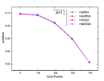
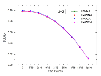
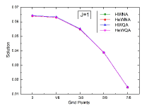
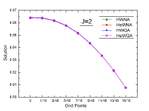
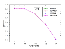
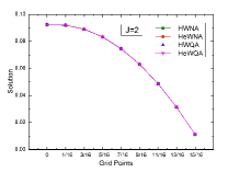
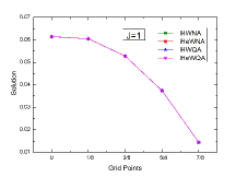
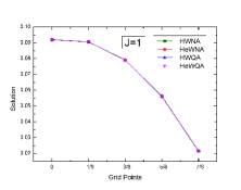
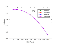
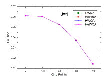
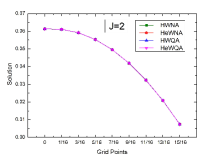
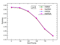
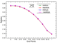
Comparison Graphs taking initial vector [0,0,,00000,0,\ldots,0] and J=1𝐽1J=1, J=2𝐽2J=2 with n=1,kg=1formulae-sequence𝑛1subscript𝑘𝑔1n=1,~{}k_{g}=1; n=1,kg=2formulae-sequence𝑛1subscript𝑘𝑔2n=1,~{}k_{g}=2; n=2,kg=1formulae-sequence𝑛2subscript𝑘𝑔1n=2,~{}k_{g}=1; n=2,kg=2formulae-sequence𝑛2subscript𝑘𝑔2n=2,~{}k_{g}=2;n=3,kg=1formulae-sequence𝑛3subscript𝑘𝑔1n=3,~{}k_{g}=1 and n=3,kg=2formulae-sequence𝑛3subscript𝑘𝑔2n=3,~{}k_{g}=2 are plotted in Figure 1, Figure 2, Figure 3, Figure 4, Figure 5 and Figure 6 respectively. Tables for solution is tabulated in table 1, 2, table 3, table 4, table 5 and table 6 respectively.

Table 1: Comparison of HWQA, HeWNA, HWQA, HeWQA method solution for example 5.1 with n=1,kg=1formulae-sequence𝑛1subscript𝑘𝑔1n=1,~{}k_{g}=1 taking J=2𝐽2J=2 :
Grid Points HWNA [29] HeWNA HWQA [29] HeWQA
0 0.098471606 0.098471868 0.099733232 0.098721649
1/16 0.098078784 0.09807895 0.099334324 0.098328004
3/16 0.094937743 0.094937908 0.096144758 0.095180981
5/16 0.08866797 0.08866813 0.089779277 0.088898418
7/16 0.079294153 0.079294305 0.080265493 0.079503596
9/16 0.066853514 0.066853646 0.067645598 0.06703223
11/16 0.051396022 0.051396117 0.051977236 0.051533416
13/16 0.032984684 0.032984721 0.033334595 0.033070901
15/16 0.011695904 0.011695851 0.011809628 0.01172465
Refer to caption
Refer to caption
Figure 1: Comparison plots of solution methods for J=1,2𝐽12J=1,2 for example 5.1 with n=1,kg=1formulae-sequence𝑛1subscript𝑘𝑔1n=1,~{}k_{g}=1:
Table 2: Comparison of HWQA, HeWNA, HWQA, HeWQA method solution for example 5.1 with n=1,kg=2formulae-sequence𝑛1subscript𝑘𝑔2n=1,~{}k_{g}=2 taking J=2𝐽2J=2 :
Grid Points HWNA [29] HeWNA HWQA [29] HeWQA
0 0.063984889 0.063981865 0.064360996 0.064044224
1/16 0.063730596 0.063727533 0.064104699 0.063789741
3/16 0.061697078 0.061694111 0.062055233 0.06175505
5/16 0.057636632 0.057633858 0.057963614 0.057691954
7/16 0.05156246 0.051559975 0.051844545 0.051613138
9/16 0.043494423 0.04349232 0.043720272 0.043537903
11/16 0.0334591 0.033457472 0.033620792 0.033492504
13/16 0.02148988 0.021488815 0.021584087 0.021510584
15/16 0.007627057 0.007626644 0.007656348 0.007633719
Refer to caption
Refer to caption
Figure 2: Comparison plots of solution methods for J=1,2𝐽12J=1,2 for example 5.1 with n=1,kg=2formulae-sequence𝑛1subscript𝑘𝑔2n=1,~{}k_{g}=2:
Table 3: Comparison of HWQA, HeWNA, HWQA, HeWQA method solution for example 5.1 with n=2,kg=1formulae-sequence𝑛2subscript𝑘𝑔1n=2,~{}k_{g}=1 taking J=2𝐽2J=2 :
Grid Points HWNA [29] HeWNA HWQA [29] HeWQA
0 0.092208342 0.092207929 0.092312756 0.092313207
1/16 0.091847576 0.091847154 0.091951987 0.091952438
3/16 0.088961585 0.088961165 0.089065836 0.089066284
5/16 0.083190705 0.08319029 0.083293585 0.083294024
7/16 0.07453702 0.074536618 0.074635444 0.074635864
9/16 0.063003362 0.06300299 0.063092011 0.063092397
11/16 0.048592958 0.048592641 0.048664618 0.048664943
13/16 0.031308953 0.031308728 0.031355798 0.031356022
15/16 0.011153812 0.011153735 0.01116988 0.011169952
Refer to caption
Refer to caption
Figure 3: Comparison plots of solution methods for example 5.1 with n=2,kg=1formulae-sequence𝑛2subscript𝑘𝑔1n=2,~{}k_{g}=1:
Table 4: Comparison of HWQA, HeWNA, HWQA, HeWQA method solution for example 5.1 with n=2,kg=2formulae-sequence𝑛2subscript𝑘𝑔2n=2,~{}k_{g}=2 taking J=2𝐽2J=2 :
Grid Points HWNA [29] HeWNA HWQA [29] HeWQA
0 0.061376073 0.061376325 0.061411277 0.061411345
1/16 0.061136122 0.061135877 0.061171325 0.061171393
3/16 0.059216558 0.05921632 0.05925171 0.059251777
5/16 0.055377823 0.055377598 0.055412494 0.055412559
7/16 0.049620654 0.049620448 0.04965375 0.049653812
9/16 0.041946044 0.041945866 0.0419757 0.041975756
11/16 0.032355109 0.032354967 0.032378845 0.032378891
13/16 0.020848901 0.020848809 0.020864147 0.020864177
15/16 0.007428191 0.007428161 0.007433258 0.007433263
Refer to caption
Refer to caption
Figure 4: Comparison plots of solution methods for J=1,2𝐽12J=1,2 for example 5.1 with n=2,kg=2formulae-sequence𝑛2subscript𝑘𝑔2n=2,~{}k_{g}=2
Table 5: Comparison of HWQA, HeWNA, HWQA, HeWQA method solution for example 5.1 with n=3,kg=1formulae-sequence𝑛3subscript𝑘𝑔1n=3,~{}k_{g}=1 taking J=2𝐽2J=2 :
Grid Points HWNA [29] HeWNA HWQA [29] HeWQA
0 0.091982324 0.091982282 0.091998157 0.091998241
1/16 0.091622975 0.091622932 0.091622975 0.091638892
3/16 0.088748193 0.08874815 0.088748193 0.088764086
5/16 0.082998726 0.082998685 0.082998726 0.083014381
7/16 0.074374752 0.074374713 0.074374752 0.07438963
9/16 0.062876486 0.062876451 0.062876486 0.062889712
11/16 0.048504139 0.048504111 0.048504139 0.048514619
13/16 0.031257869 0.031257851 0.031257869 0.031264554
15/16 0.011137751 0.011137745 0.011137751 0.011139994
Refer to caption
Refer to caption
Figure 5: Comparison plots of solution methods for J=1,2𝐽12J=1,2 for example 5.1 with n=3,kg=1formulae-sequence𝑛3subscript𝑘𝑔1n=3,~{}k_{g}=1
Table 6: Comparison of HWQA, HeWNA, HWQA, HeWQA method solution for example 5.1 with n=3,kg=2formulae-sequence𝑛3subscript𝑘𝑔2n=3,~{}k_{g}=2 taking J=2𝐽2J=2:
Grid Points HWNA [29] HeWNA HWQA [29] HeWQA
0 0.061315351 0.061315829 0.061318845 0.061321705
1/16 0.061075828 0.061075814 0.061079322 0.061083071
3/16 0.059159646 0.059159634 0.059163135 0.059166226
5/16 0.055327307 0.055327295 0.055330739 0.055333256
7/16 0.049578851 0.04957884 0.049582101 0.049584212
9/16 0.041914328 0.041914319 0.041917195 0.041918897
11/16 0.032333785 0.032333778 0.032336026 0.032337266
13/16 0.020837254 0.02083725 0.020838652 0.020839592
15/16 0.007424747 0.007424746 0.007425199 0.007424945
Refer to caption
Refer to caption
Figure 6: Comparison plots of solution methods for J=1,2𝐽12J=1,2 for example 5.1 with n=3,kg=2formulae-sequence𝑛3subscript𝑘𝑔2n=3,~{}k_{g}=2

The example defined by equation (102) is new and does not exist in literature. So we are not in a situation to compare the results. We have considered n=1,2,3𝑛123n=1,2,3 and kg=1,2subscript𝑘𝑔12k_{g}=1,2. Tables 1, 2, 3, 4, 5 , 6 and figures 1, 2, 3, 4, 5, 6 demonstrate the behaviour of the solution for J=1,2𝐽12J=1,2. HWNA, HeWNA, HWQA and HeWQA all give numerics which are very well comparable and shows that our proposed techniques are working well.

We also observed for small changes in initial vector, for example taking [0.1,0.1,,0.1]0.10.10.1[0.1,0.1,\ldots,0.1] or [0.2,0.2,,0.2]0.20.20.2[0.2,0.2,\ldots,0.2] doesn’t significantly change the solution in any case.

5.2 Example 2 (Stellar Structure)

Consider the non-linear SBVP:

Ly(t)+y5(t)=0,y(0)=0,y(1)=34,kg=2,formulae-sequence𝐿𝑦𝑡superscript𝑦5𝑡0formulae-sequencesuperscript𝑦00formulae-sequence𝑦134subscript𝑘𝑔2\displaystyle Ly(t)+y^{5}(t)=0,\quad y^{\prime}(0)=0,\quad y(1)=\sqrt{\frac{3}{4}},\quad k_{g}=2, (103)

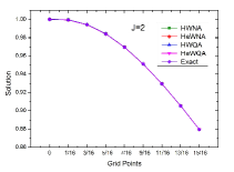
Chandrasekhar ([5], p88 ) derived above two point nonlinear SBVP. This equation arise in study of stellar structure. Its exact solution is y(t)=33+x2𝑦𝑡33superscript𝑥2y(t)=\sqrt{\frac{3}{3+x^{2}}}.

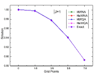
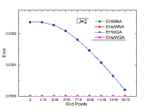
Comparison Graphs taking initial vector [34,34,,34343434\sqrt{\frac{3}{4}},\sqrt{\frac{3}{4}},\ldots,\sqrt{\frac{3}{4}}] and J=1𝐽1J=1, J=2𝐽2J=2 are plotted in Figure 7. Tables for solution and error are tabulated in table 7 and table 8.

Table 7: Comparison of HWNA, HeWNA, HWQA, HeWQA methods solution with analytical solution for example 5.2 taking J=2𝐽2J=2 :
Grid Points HWNA [29] HeWNA HWQA [29] HeWQA Exact
0 1.00023666 0.999999992 1.00023666 0.999999992 1
1/16 0.999586961 0.99934958 0.999586961 0.99934958 0.999349593
3/16 0.994419294 0.994191616 0.994419294 0.994191616 0.994191626
5/16 0.984319576 0.984110835 0.984319576 0.984110835 0.984110842
7/16 0.969730094 0.96954859 0.969730094 0.96954859 0.969548596
9/16 0.9512486 0.951101273 0.9512486 0.951101273 0.951101277
11/16 0.92956584 0.92945791 0.92956584 0.92945791 0.929457914
13/16 0.905403371 0.905338132 0.905403371 0.905338132 0.905338136
15/16 0.879460746 0.879439538 0.879460746 0.879439538 0.879439536
Table 8: Comparison of error of HWNA, HeWNA, HWQA, HeWQA methods for example 5.2 taking J=2𝐽2J=2 :
Error HWNA [29] HeWNA HWQA [29] HeWQA
Lsubscript𝐿L_{\infty} 0.000237368 2.49669×10⁹absentsuperscript109\times 10^{-9} 0.000237368 2.49669×10⁹absentsuperscript109\times 10^{-9}
L2subscript𝐿2L_{2} 0.000471959 1.97638×10⁸absentsuperscript108\times 10^{-8} 0.000471959 1.97638×10⁸absentsuperscript108\times 10^{-8}
Refer to caption
Refer to caption
Refer to caption
Refer to caption
Figure 7: Comparison plots and error plots of solution methods for J=1,2𝐽12J=1,2 for example 5.2

In this test case since exact solution of the SBVP governed by (103) exists, We have compared our solutions with exact solution in table 7 and figure 7. Numerics again prove that method gives results with best accuracy for J=1𝐽1J=1 and J=2𝐽2J=2.

We also observed for small changes in initial vector, for example taking [0.8,0.8,,0.8]0.80.80.8[0.8,0.8,\ldots,0.8] or [0.7,0.7,,0.7]0.70.70.7[0.7,0.7,\ldots,0.7] doesn’t significantly change the solution.

5.3 Example 3 (Thermal Explosion)

Consider the non linear SBVP:

Ly(t)+ey(t)=0,y(0)=0,y(1)=0,kg=1.formulae-sequence𝐿𝑦𝑡superscript𝑒𝑦𝑡0formulae-sequencesuperscript𝑦00formulae-sequence𝑦10subscript𝑘𝑔1\displaystyle Ly(t)+e^{y(t)}=0,\quad y^{\prime}(0)=0,\quad y(1)=0,~{}k_{g}=1. (104)

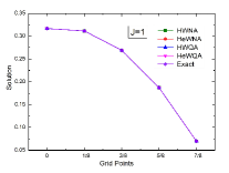
Above nonlinear SBVP is derived by Chamber [4]. This equation arises in the thermal explosion in cylindrical vessel. The exact solution of this equation is y(x)=2ln422(322)x2+1𝑦𝑥2422322superscript𝑥21y(x)=2\ln{\frac{4-2\sqrt{2}}{(3-2\sqrt{2})x^{2}+1}}.

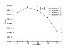
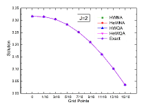
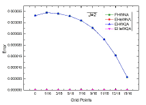
Comparison Graphs taking initial vector [0,0,,00000,0,\ldots,0] and J=1𝐽1J=1, J=2𝐽2J=2 are plotted in Figure 8. Tables for solution and error are tabulated in table 9 and table 10.

Table 9: Comparison of HWNA, HeWNA, HWQA, HeWQA methods solution with analytical solution for example 5.3 taking J=2𝐽2J=2:
Grid Points HWNA [29] HeWNA HWQA [29] HeWQA Exact
0 0.316727578 0.316694368 0.316727578 0.316694368 0.316694368
1/16 0.315388914 0.315354403 0.315388914 0.315354403 0.315354404
3/16 0.304700946 0.304666887 0.304700946 0.304666887 0.304666888
5/16 0.283494667 0.283461679 0.283494667 0.283461679 0.283461679
7/16 0.252100547 0.252069555 0.252100547 0.252069555 0.252069555
9/16 0.210993138 0.210965461 0.210993138 0.210965461 0.210965462
11/16 0.160768168 0.16074555 0.160768168 0.16074555 0.16074555
13/16 0.102115684 0.102100258 0.102115684 0.102100258 0.102100258
15/16 0.035791587 0.035785793 0.035791587 0.035785793 0.035785793
Table 10: Comparison of error of HWNA, HeWNA, HWQA, HeWQA methods for example 5.3 taking J=2𝐽2J=2 :
Error HWNA [29] HeWNA HWQA [29] HeWQA
Lsubscript𝐿L_{\infty} 0.0000345103 1.07541×10¹⁰absentsuperscript1010\times 10^{-10} 0.0000345103 1.07541×10¹⁰absentsuperscript1010\times 10^{-10}
L2subscript𝐿2L_{2} 0.0000771278 4.99369×10¹⁰absentsuperscript1010\times 10^{-10} 0.0000771278 4.99369×10¹⁰absentsuperscript1010\times 10^{-10}
Refer to caption
Refer to caption
Refer to caption
Refer to caption
Figure 8: Comparison plot and error plots of solution methods for J=1,2𝐽12J=1,2 for example 5.3

This is test case derived by Chambre [4] long back again exact solution is available. Table 9 and figure 8 show that numerics are in good agreement with exact solutions or J=1𝐽1J=1 and J=2𝐽2J=2.

We also observed for small changes in initial vector, for example taking [0.1,0.1,,0.1]0.10.10.1[0.1,0.1,\ldots,0.1] or [0.2,0.2,,0.2]0.20.20.2[0.2,0.2,\ldots,0.2] doesn’t significantly change the solution.

5.4 Example 4 (Rotationally Symmetric Shallow Membrane Caps)

Consider the non linear SBVP:

Ly(t)+(18y2(t)12)=0,y(0)=0,y(1)=1,kg=1.formulae-sequence𝐿𝑦𝑡18superscript𝑦2𝑡120formulae-sequencesuperscript𝑦00formulae-sequence𝑦11subscript𝑘𝑔1\displaystyle Ly(t)+\left(\frac{1}{8y^{2}(t)}-\frac{1}{2}\right)=0,\quad y^{\prime}(0)=0,\quad y(1)=1,~{}k_{g}=1. (105)

Above nonlinear SBVP is studied in papers [7, 3]. Exact solution of this problem is not known.

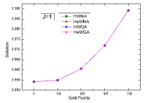
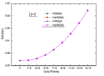
Comparison Graphs taking initial vector [1,1,,11111,1,\ldots,1] and J=1𝐽1J=1, J=2𝐽2J=2 are plotted in Figure 9. Tables for solution is tabulated in table 11.

Table 11: Comparison of HWQA, HeWNA, HWQA, HeWQA method solution for example 5.4 taking J=2𝐽2J=2:
Grid Points HWNA [29] HeWNA HWQA [29] HeWQA
0 0.954137376 0.954135008 0.954137376 0.954135008
1/16 0.954314498 0.954311604 0.954314498 0.954311604
3/16 0.95573187 0.95572956 0.95573187 0.95572956
5/16 0.958569785 0.958567713 0.958569785 0.958567713
7/16 0.962834546 0.962832683 0.962834546 0.962832683
9/16 0.968535496 0.968533886 0.968535496 0.968533886
11/16 0.975684891 0.975683641 0.975684891 0.975683641
13/16 0.984297738 0.984296771 0.984297738 0.984296771
15/16 0.994391588 0.994391728 0.994391588 0.994391728
Refer to caption
Refer to caption
Figure 9: Comparison plots of solution methods for J=1,2𝐽12J=1,2 for example 5.4

In this real life example again exact solution is not known so comparison is not done with exact solution. Table 11 and figure 9 show that computed results are comparable for J=1,2𝐽12J=1,2.

We also observed for small changes in initial vector, for example taking [0.9,0.9,,0.9]0.90.90.9[0.9,0.9,\ldots,0.9] or [0.8,0.8,,0.8]0.80.80.8[0.8,0.8,\ldots,0.8] doesn’t significantly change the solution.

5.5 Example 5 (Thermal Distribution in Human Head)

Consider the non linear SBVP:

Ly(t)+ey(t)=0,y(0)=0,2y(1)+y(1)=0,kg=2.formulae-sequence𝐿𝑦𝑡superscript𝑒𝑦𝑡0formulae-sequencesuperscript𝑦00formulae-sequence2𝑦1superscript𝑦10subscript𝑘𝑔2\displaystyle Ly(t)+e^{-y(t)}=0,\quad y^{\prime}(0)=0,\quad 2y(1)+y^{\prime}(1)=0,~{}k_{g}=2. (106)

This SBVP is derived by Duggan and Goodman [8]. Exact solution of this problem is not known to the best of our knowledge.

Comparison Graphs taking initial vector [0,0,,00000,0,\ldots,0] and J=1𝐽1J=1, J=2𝐽2J=2 are plotted in Figure 10. Tables for solution is tabulated in table 12.

Table 12: Comparison of HWQA, HeWNA, HWQA, HeWQA method solution for example 5.5 taking J=2𝐽2J=2:
Grid Points HWNA [29] HeWNA HWQA [29] HeWQA
0 0.269855704 0.269948774 0.272263769 0.272366612
1/16 0.269358573 0.269451863 0.27176762 0.271870738
3/16 0.265377954 0.265471233 0.267793921 0.267896983
5/16 0.257388082 0.257481347 0.259810468 0.259913411
7/16 0.245331028 0.245424295 0.247745058 0.247847809
9/16 0.229118226 0.229211536 0.231489202 0.231591678
11/16 0.208628362 0.2087218 0.210897975 0.211000089
13/16 0.183704413 0.183798121 0.18579005 0.18589165
15/16 0.154149664 0.154243862 0.155947881 0.156048741
1 0.13756259 0.137656718 0.139174003 0.139274111
Refer to caption
Refer to caption
Figure 10: Comparison plots of solution methods for J=1,2𝐽12J=1,2 for example 5.5

In absence of exact solution the comparison has not been made with exact solution. But comparison of all four methods for in the given problem due to Duggan and Goodman [8], in table 12 and figure 10 shows accuracy of the present method.

We also observed for small changes in initial vector, for example taking [0.1,0.1,,0.1]0.10.10.1[0.1,0.1,\ldots,0.1] or [0.2,0.2,,0.2]0.20.20.2[0.2,0.2,\ldots,0.2] doesn’t significantly change the solution in any case.

6 Conclusions

In this research article, we have proposed a new model governing exothermic reactions and four different numerical methods based on wavelets, namely HWQA, HWNA, HeWQA, HeWNA for solving these nonlinear SBVPs arising in different branches of science and engineering (cf. [7, 3, 8, 4, 5]). We have applied these methods in five real life examples [see equations (102), (103), (104), (105) and (106)]. Singularity of differential equations can also be very well handled with help of these four proposed methods based. Difficulty arise due to non-linearity of differential equations is dealt with the help of quasilinearization in HWQA and HeWQA method. In the other two proposed method, HWNA and HeWNA, we will solve the resulting non-linear system with help of Newton-Raphson method. Boundary conditions are also handled well by the proposed methods. Main advantage of proposed methods is that solutions with high accuracy are obtained using a few iterations. We also observe that small perturbation in initial vector does not significantly change the solution. Which shows that our method is numerically stable.

Our convergence analysis shows that that Ek,Mnormsubscript𝐸𝑘𝑀||E_{k,M}|| tends to zero as M𝑀M tends to infinite. Which shows that accuracy of solution increases as J𝐽J increases.

Computational work illustrate the validity and accuracy of the procedure. Our computations are based on a higher resolution and codes developed can easily be used for even further resolutions.

References

  • [1] S. Saha Ray A. K. Gupta. An investigation with hermite wavelets for accurate solution of fractional jaulent–miodek equation associated with energy-dependent schrödinger potential. Applied Mathematics and Computation, 270:458–471, 2015.
  • [2] Pouria Assari and Mehdi Dehghan. Application of dual-chebyshev wavelets for the numerical solution of boundary integral equations with logarithmic singular kernels. Engineering with Computers, 35(1):175–190, Jan 2019.
  • [3] John V. Baxley and Stephen B. Robinson. Nonlinear boundary value problems for shallow membrane caps, ii. Journal of Computational and Applied Mathematics, 88:203 – 224, 1998.
  • [4] P. L. Chambre. On the solution of the poisson‐boltzmann equation with application to the theory of thermal explosions. The Journal of Chemical Physics, 20(11):1795–1797, 1952.
  • [5] S. Chandrasekhar. Introduction to the study of stellar structure. Dover publications, 1967.
  • [6] C. F. Chen and C. H. Hsiao. Haar wavelet method for solving lumped and distributed-parameter systems. IEEE Proceedings Control Theory and Applications, 144:87 – 94, 1997.
  • [7] R. W. Dickey. Rotationally symmetric solutions for shallow membrane caps. Quarterly of Applied Mathematics, 47:571–581, 1989.
  • [8] R. C. Duggan and A. M. Goodman. Pointwise bounds for a nonlinear heat conduction model of the human head. Bulletin of Mathematical Biology, 48:229 – 236, 1986.
  • [9] G. Hariharan. An Efficient Wavelet-Based Spectral Method to Singular Boundary Value Problems, pages 63–91. Springer Singapore, Singapore, 2019.
  • [10] Harpreet Kaur, R.C . Mittal, and Vinod Mishra. Haar wavelet approximate solutions for the generalized laneemden equations arising in astrophysics. Computer Physics Communications, 184:2169–2177, 2013.
  • [11] Hassan Khan, Muhammad Arif, and Syed Tauseef Mohyud-Din. Numerical Solution Of Fractional Boundary Value Problems By Using Chebyshev Wavelet. Matrix Science Mathematic (MSMK), 3(1):13–16, March 2019.
  • [12] Ulo Lepik. Haar wavelet method for solving higher order differential equations. International Journal of Mathematics and Computation, 1:84–94, 2008.
  • [13] Stephane G. Mallat. Multiresolution approximations and wavelet orthonormal bases of l2(𝐫)superscript𝑙2𝐫l^{2}({\bf r}). Trans. Amer. Math. Soc., 315:69–87, 1989.
  • [14] F. Mohammadi and M.M. Hosseini. A new legendre wavelet operational matrix of derivative and its applications in solving the singular ordinary differential equations. Journal of the Franklin Institute, 348(8):1787 – 1796, 2011.
  • [15] Kazutaka Nakamura, Toshiyuki Takayanagi, and Shin Sato. A modified arrhenius equation. Chemical Physics Letters, 160(3):295 – 298, 1989.
  • [16] A. Kazemi Nasab, A. Kılıçman, E. Babolian, and Z. Pashazadeh Atabakan. Wavelet analysis method for solving linear and nonlinear singular boundary value problems. Applied Mathematical Modelling, 37(8):5876 – 5886, 2013.
  • [17] R.K. Pandey and A.K. Verma. Existence-uniqueness results for a class of singular boundary value problems arising in physiology. Nonlinear Analysis: Real World Applications, 9(1):40 – 52, 2008.
  • [18] R.K. Pandey and A.K. Verma. Existence-uniqueness results for a class of singular boundary value problems-ii. Journal of Mathematical Analysis and Applications, 338(2):1387 – 1396, 2008.
  • [19] R.K. Pandey and A.K. Verma. A note on existence-uniqueness results for a class of doubly singular boundary value problems. Nonlinear Analysis: Theory, Methods & Applications, 71(7):3477 – 3487, 2009.
  • [20] María Cristina Pereyra and Lesley A. Ward. Harmonic Analysis: From Fourier to Wavelets. 2012.
  • [21] Umer Saeed and Mujeeb ur Rehman. Hermite wavelet method for fractional delay differential equations. Journal of Difference Equations, 2014, 2014.
  • [22] S. C. Shiralashetti and S. Kumbinarasaiah. Hermite wavelets operational matrix of integration for the numerical solution of nonlinear singular initial value problems. Alexandria Engineering Journal, 2017.
  • [23] Kumbinarasaiah Srinivasa Siddu Channabasappa Shiralashetti. Hermite wavelets method for the numerical solution of linear and nonlinear singular initial and boundary value problems. Computational Methods for Differential Equations, 7(2):177–198, 2019.
  • [24] Mandeep Singh, Verma Amit K., and Ravi P. Agarwal. On an iterative method for a class of 2 point & 3 point nonlinear sbvps. Journal of Applied Analysis and Computation, 9(4):1242–1260, 2019.
  • [25] Mandeep Singh and Amit K. Verma. An effective computational technique for a class of lane–emden equations. Journal of Mathematical Chemistry, 54(1):231–251, Jan 2016.
  • [26] R. Singh, J. Shahni nd H. Garg, and A. Garg. Haar wavelet collocation approach for lane-emden equations arising in mathematical physics and astrophysics. The European Physical Journal Plus, 2019.
  • [27] Randhir Singh, Himanshu Garg, and Vandana Guleria. Haar wavelet collocation method for lane–emden equations with dirichlet, neumann and neumann–robin boundary conditions. Journal of Computational and Applied Mathematics, 346:150 – 161, 2019.
  • [28] Amit K. Verma. The monotone iterative method and zeros of bessel functions for nonlinear singular derivative dependent bvp in the presence of upper and lower solutions. Nonlinear Analysis: Theory, Methods & Applications, 74(14):4709 – 4717, 2011.
  • [29] Amit K. Verma and Diksha Tiwari. Higher resolution methods based on quasilinearization and haar wavelets on lane–emden equations. International Journal of Wavelets, Multiresolution and Information Processing, 17(3):1950005, 2019.
  • [30] Amit Kumar Verma and Sheerin Kayenat. On the convergence of mickens’ type nonstandard finite difference schemes on lane-emden type equations. Journal of Mathematical Chemistry, 56(6):1667–1706, Jun 2018.
  • [31] Fengying Zhou and Xiaoyong Xu. Numerical solutions for the linear and nonlinear singular boundary value problems using laguerre wavelets. Advances in Difference Equations, 2016(1):17, 2016.