Exceptional points of the eigenvalues of parameter-dependent Hamiltonian operators

Abstract

We calculate the exceptional points of the eigenvalues of several parameter-dependent Hamiltonian operators of mathematical and physical interest. We show that the calculation is greatly facilitated by the application of the discriminant to the secular determinant. In this way the problem reduces to finding the roots of a polynomial function of just one variable, the parameter in the Hamiltonian operator. As illustrative examples we consider a particle in a one-dimensional box with a polynomial potential, the periodic Mathieu equation, the Stark effect in a polar rigid rotor and in a polar symmetric top.

1 Introduction

In many applications of quantum mechanics to physical problems the Hamiltonian operator $H(\lambda)$ depends on a parameter $\lambda$. For example, in the case of atoms and molecules in electric or magnetic fields the parameter $\lambda$ is related to the intensity of the external field so that $H(0)$ is the Hamiltonian operator for the isolated atom or molecule. One of the approximate methods for calculating the energies $E(\lambda)$ of such problems is perturbation theory that is based on the Taylor expansion of the energies $E(\lambda)$ and eigenfunctions $\psi(\lambda)$ about $\lambda=0$. The resulting series may be divergent or they may have finite convergent radii[1, 2, 3] (and references therein).

When $H(\lambda)$ is an analytic function of $\lambda$ (the typical case being $H(\lambda)=H_{0}+\lambda H^{\prime}$) the convergence of the perturbation series radii are determined by exceptional points (EPS) in the complex $\lambda$ plane where two or more eigenvalues coalesce. This coalescence is different from degeneracy in that the corresponding eigenvectors become linear dependent at an EP. For this reason there has been great interest in the accurate calculation of EPS. Among the models analyzed are the Mathieu equation[4, 5, 6, 7, 8, 9, 10, 11], a polar rigid rotor in an electric field[12, 11], a polar symmetric top in an electric field[7, 13] and a particle in a box with a linear potential[11]. In all those cases only a pair of eigenvalues coalesce at each EP that is also called a branch point, double point or critical point. The EPS on the imaginary axis proved to be relevant to the study of $\mathcal{PT}$-symmetric non-Hermitian Hamiltonians[11] (and references therein).

The EPS can be estimated by a suitable analysis of the perturbation series[7, 3] but there are more accurate techniques[3, 4, 5, 6, 8, 9, 10, 11], most of which are based on the secular equation for a truncated matrix representation of the Hamiltonian operator in a suitable basis set of eigenvectors. In most of these cases, one obtains the eigenvalues $E(\lambda)$ from the roots of a nonlinear equation $Q(E,\lambda)=0$ and it is well known that the branch points are simultaneous solution of this equation and $\partial$ $Q(E,\lambda)/\partial E=0$. This approach and its variants[3, 4, 5, 6, 8, 9, 10, 11] have proved suitable for the calculation of reasonably accurate EPS. However, finding the roots of two nonlinear equations requires a judicious application of efficient algorithms (see, for example, the remarkable calculation of double points carried out many years ago for the characteristic values of the Mathieu equation[4]).

The purpose of this paper is to point out that the calculation of the EPS is considerably facilitated by the application of the discriminant[14, 15, 26, 16] to the polynomial function that determines the approximate energies of the quantum-mechanical problem. The advantage is that the two nonlinear equations in two variables reduce to one nonlinear equation in one variable. As a result, the estimation of the EPS reduces to the calculation of the roots of one nonlinear equation in the parameter $\lambda$. Another advantage of this approach is that most computer-algebra software have built-in algorithms for the calculation of the discriminant of a polynomial. The resultant of two polynomials and the discriminant of a polynomial are known since long ago in the mathematical literature[14, 15, 26, 16] and have already been applied to the analysis of physical problems. Some of the examples are the determination of singularities in the eigenvalues of parameter-dependent matrix eigenvalue problems[18], the analysis of the properties of two-dimensional magnetic traps for laser-cooled atoms[19], the description of optical polarization singularities[20], the EPS for the eigenvalues of a modified Lipkin model[21], the location of level crossings between eigenvalues of parameter-dependent symmetric matrices[22, 23, 24, 25], the solution of two equations with two unknowns that appear in the study of gravitational lenses[26]. In all these applications the resultant and discriminant have been applied to polynomials of finite degree coming from matrices of finite dimension where the technique yields exact results. In this paper, on the other hand, we focus on quantum-mechanical problems defined on infinite Hilbert spaces so that the matrix representations of the Hamiltonian operators and their characteristic polynomials are approximate due to necessary truncation.

In section 2 we briefly discuss some properties of parameter-dependent Hamiltonians, in section 3 we apply the approach to a particle in a box with two different potentials, in section 4 we consider the periodic solutions to the Mathieu function, sections 5 and 6 are devoted to the Stark effect in a polar rigid rotor and a symmetric top, respectively. Finally, in section 7 we summarize the main results and draw conclusions. In order to make this paper sufficiently self-contained we add two appendices with a discussion of three-term recurrence relations for the expansion coefficients of the wavefunctions and a slight introduction to the resultant of two polynomials and the discriminant of a polynomial.

2 Parameter-dependent Hamiltonians

The purpose of this paper is the analysis of Hamiltonian operators $H(\lambda)$ that depend on a parameter $\lambda$. Their eigenvalues $E_{n}(\lambda)$ and eigenvectors (or eigenfunctions) $\psi_{n}$ depend on this parameter. This kind of problems may exhibit EPS $\lambda_{EP}$ in the complex $\lambda$-plane at which two (or more) eigenvalues coalesce: $E_{m}\left(\lambda_{EP}\right)=E_{n}\left(\lambda_{EP}\right)$. This phenomenon is different from ordinary degeneracy in that the corresponding eigenvectors $\psi_{m}$ and $\psi_{n}$ become linearly dependent at an exceptional point $\lambda_{EP}$. If we manage to obtain a power-series expansion

$$E_{n}(\lambda)=\sum_{j=0}E_{n,j}\lambda^{j},$$ (1)

for example by means of perturbation theory, its radius of convergence will be determined by the EP closest to the origin of the complex $\lambda$-plane[1, 2, 3].

One can obtain EPS from a nonlinear equation of the form $Q(E,\lambda)=0$, from which one commonly obtains the eigenvalues $E_{n}(\lambda)$. It is well known that the branch points of the eigenvalues as functions of the complex parameter $\lambda$ are common roots of the nonlinear equations $\left\{Q(E,\lambda)=0,\partial Q(E,\lambda)/\partial E=0\right\}$. In this paper we consider a simple and straightforward way of obtaining the EPS that enables one to reduce the two nonlinear equations of two variables to just one nonlinear function of $\lambda$.

One of the simplest ways of obtaining the equation $Q(E,\lambda)=0$ is based on the matrix representation $\mathbf{H}$ of the Hamiltonian operator $H$ in a given orthonormal basis set $\left\{\left|i\right\rangle,i=0,1,\ldots\right\}$. If the basis set is infinite we resort to an approximate truncated matrix representation $\mathbf{H}_{N}$ with elements $H_{ij}=\left\langle i\right|H\left|j\right\rangle$, $i,j=0,1,\ldots,N-1$. The approximate energies are roots of the characteristic polynomial

$$p_{N}(E,\lambda)=\left|\mathbf{H}_{N}-E\mathbf{I}_{N}\right|=0,$$ (2)

where $\mathbf{I}_{N}$ is the $N\times N$ identity matrix. The roots of $p_{N}(E,\lambda)=0$ give us approximate eigenvalues $E_{n}(\lambda)$ and, consequently, we expect to obtain the EPS with increasing accuracy by increasing $N$.

Since the EPS are complex values of $\lambda$ for which two eigenvalues coalesce, and taking into account that $p_{N}(E,\lambda)$ is a polynomial function of $E$, it is clear from the discussion of the discriminant in A that the EPS can be obtained from the roots $\lambda_{i}^{[N]}$ of the one-variable function

$$F_{N}(\lambda)=Disc_{E}\left(p_{N}(E,\lambda)\right).$$ (3)

Since the characteristic polynomial comes from a truncation of the matrix representation of the Hamiltonian, one expects some of the roots of $F_{N}(\lambda)$ to be spurious. However, the sequences of roots that converge when $N$ increases are expected to yield the actual EPS. Another advantage of this approach is that most computer-algebra software have built-in algorithms for the calculation of the discriminant of a polynomial. It is worth noticing that this approach applies even in the case that more than two eigenvalues coalesce at an EP (see A). The approach just outlined is particularly simple and practical when $H=H_{0}+\lambda H^{\prime}$ because in this case $F_{N}(\lambda)$ is a polynomial function of $\lambda$.

Suppose that $E(0)$ is an isolated simple eigenvalue of $H_{0}$ and that there are two real numbers $a$ and $b$ such that

$$\left\|H^{\prime}\Phi\right\|\leq a\left\|H_{0}\Phi\right\|+b\left\|\Phi\right\|,$$ (4)

where $\left\|f\right\|=\sqrt{\left\langle f\right|\left.f\right\rangle}$, for all $\Phi$ in the state space. Under such conditions there is a unique eigenvalue $E(\lambda)$ of $H$ near $E(0)$ and $E(\lambda)$ is analytic in a neighbourhood of $\lambda=0$ in the complex $\lambda$ plane[1, 2, 3] (and references therein). All the examples discussed in this paper satisfy this condition because $\left\|H^{\prime}\Phi\right\|\leq b\left\|\Phi\right\|$ as we will see below.

If $H(\lambda)$ is Hermitian for $\lambda$ real, then the EPS cannot be real. In all the examples discussed here $H(\lambda)^{\ast}=H(\lambda^{\ast})$ for $\lambda$ complex so that $H(\lambda^{\ast})\psi_{n}^{\ast}=E_{n}(\lambda)^{\ast}\psi_{n}^{\ast}$ and, consequently, $E_{n}(\lambda)^{\ast}=E_{m}(\lambda^{\ast})$. Suppose that $E_{n}(\lambda)$ and $E_{k}(\lambda)$ coalesce at $\lambda_{EP}$, therefore $E_{n}\left(\lambda_{EP}\right)^{\ast}=E_{k}\left(\lambda_{EP}\right)^{\ast}\Rightarrow E_{m}\left(\lambda_{EP}^{\ast}\right)=E_{j}\left(\lambda_{EP}^{\ast}\right)$ and, by virtue of the preceding result, $\lambda_{EP}^{\ast}$ is also an EP. In other words, the EPS appear in pairs of complex-conjugate numbers.

Suppose that there exists a unitary operator $U$ such that $U^{\dagger}H(\lambda)U=H(-\lambda)$; therefore $U^{\dagger}H(\lambda)\psi_{n}=H(-\lambda)U^{\dagger}\psi_{n}=E_{n}(\lambda)U^{\dagger}\psi_{n}$, from which it follows that $E_{n}(\lambda)=E_{m}(-\lambda)$. We conclude that if $\lambda_{EP}$ is an EP, then $-\lambda_{EP}$ is also an EP. It follows from the two preceding results that there may be quadruplets of EPS: $\lambda_{EP}$, $\lambda_{EP}^{\ast}$, $-\lambda_{EP}$ and $-\lambda_{EP}^{\ast}$ when $\Re\lambda_{EP}\neq 0$.

3 Particle in a one-dimensional box with a perturbation

Our first example is given by a particle in a one-dimensional box with an interaction potential. The Schrödinger equation for such a problem can be written in dimensionless form as

$$-\psi^{\prime\prime}(x)+\lambda V(x)\psi(x)=E\psi(x),$$

$$\psi(-1)=\psi(1)=0.$$ (5)

If $V(x)=H^{\prime}$ is a continuous function of $x$ then $\left|V(x)\right|\leq C$ when $x\in(-1,1)$ and $\left\|H^{\prime}\Phi\right\|\leq C^{2}\left\|\Phi\right\|$. Consequently, every eigenvalue $E_{n}(\lambda)$ is an analytical function of $\lambda$ for all $\lambda<\left|\lambda_{EP}\right|$, where $\lambda_{EP}$ is the EP closest to the origin of the complex $\lambda$ plane. In order to obtain a suitable matrix representation for this Hamiltonian we resort to the basis set of eigenfunctions of $H_{0}=-d^{2}/dx^{2}$:

$$\left\langle x\right.\left|n\right\rangle=\sin\left(\frac{(n+1)\pi(x+1)}{2}\right),\;n=0,1,\ldots.$$ (6)

If $V(x)$ is a polynomial function of $x$ the analytical calculation of its matrix elements $\left\langle m\right|V\left|n\right\rangle$ is straightforward. The simplest example is $V(x)=x$. The canonical transformation $U^{\dagger}xU=-x$, $U^{\dagger}d/dxU=-d/dx$ yields $U^{\dagger}H(\lambda)U=H(-\lambda)$ and, therefore, we expect the EPS to appear as quadruplets ($\Re\lambda_{EP}\neq 0$) and doublets ($\Re\lambda_{EP}=0$).

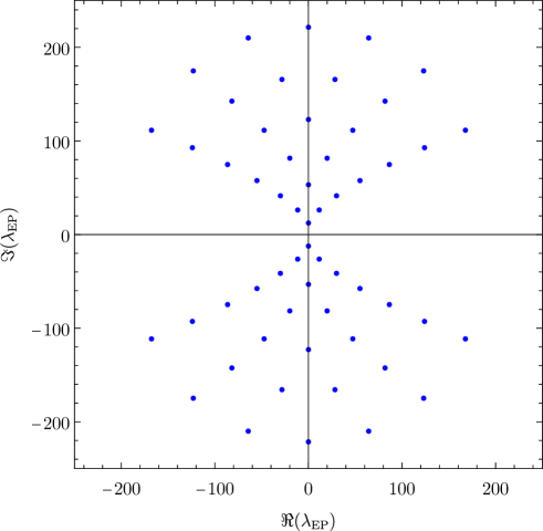
Figure 1: EPS for the particle in a box with potential $\lambda x$

In order to discard any spurious root $\lambda_{i}^{[N]}$ of the polynomial $F_{N}(\lambda)$ of degree $N(N-1)$ we keep only those that satisfy $\left|\lambda_{EP}^{[N]}-\lambda_{EP}^{[N-1]}\right|<10^{-3}$. Figure 1 shows some of the EPS for this problem; they clearly exhibit the symmetry just mentioned with respect to the real ($\lambda_{EP}$,$\lambda_{EP}^{\ast}$) and imaginary ($\lambda_{EP}$,$-\lambda_{EP}$) axes of the complex $\lambda$ plane. A larger number of EPS on the imaginary axis was obtained recently in a study of $\mathcal{PT}$-symmetric non-Hermitian Hamiltonians[11].

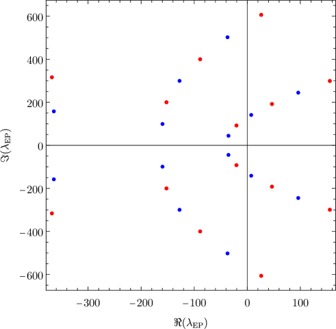
Figure 2: EPS for the particle in a box with potential $\lambda x^{2}$ for even (blue circles) and odd (red circles) states

If $V(x)=x^{2}$ the canonical transformation discussed above leaves $H(\lambda)$ invariant and we only expect doublets (that is to say: symmetry with respect to the real axis). Figure 2 confirms this conclusion. In this case it is convenient to treat the even ($n=0,2,\ldots$) and odd states ($n=1,3,\ldots$) separately.

4 Mathieu equation

One of the most widely studied periodic problems is the Mathieu equation that we write here in the following form

$$\psi^{\prime\prime}(x)+\left[E-2\lambda\cos(2x)\right]\psi(x)=0,$$ (7)

so that we can relate it to the linear operator $H=-d^{2}/dx^{2}+2\lambda\cos(2x)$. We consider the two cases of periodic solutions, those of period $\pi$ ($\psi(x+\pi)=\psi(x)$) and those of period $2\pi$ ($\psi(x+2\pi)=\psi(x)$) and each class can be separated into even and odd. The four cases can be reduced to tridiagonal matrix representations or three-term recurrence relations; in what follows we show the main parameters (see B) for each of them.

Period $\pi$ even:

$$\left|j\right\rangle = \frac{\sqrt{2}+\left(1-\sqrt{2}\right)\delta_{j0}}{\sqrt{\pi}}\cos(2jx),\;j=0,1,\ldots,$$

$$A_{j+1} = \left[1+\left(\sqrt{2}-1\right)\delta_{j0}\right]\lambda,\;B_{j}=4j^{2}-E.$$ (8)

Period $\pi$ odd

$$\left|j\right\rangle = \sqrt{\frac{2}{\pi}}\sin[(2j+2)x],\;j=0,1,\ldots,$$

$$A_{j+1} = \lambda,\;B_{j}=4(j+1)^{2}-E.$$ (9)

Period $2\pi$ even

$$\left|j\right\rangle = \sqrt{\frac{2}{\pi}}\cos\left[(2j+1)x\right],\;j=0,1,\ldots,$$

$$A_{j+1} = \lambda,\;B_{j}=(2j+1)^{2}+\lambda\delta_{j0}-E.$$ (10)

Period $2\pi$ odd

$$\left|j\right\rangle = \sqrt{\frac{2}{\pi}}\sin\left[(2j+1)x\right],\;j=0,1,\ldots,$$

$$A_{j+1} = \lambda,\;B_{j}=(2j+1)^{2}-\lambda\delta_{j0}-E.$$ (11)

In all these cases we find that $\left\|H^{\prime}\Phi\right\|\leq\left\|H^{\prime}\Phi\right\|$ because $\left|H^{\prime}\right|=\left|\cos(2x)\right|\leq 1$. Besides, the canonical transformation $U^{\dagger}xU=x+\pi/2$, $U^{\dagger}d/dxU=d/dx$ leads to $U^{\dagger}H(\lambda)U=H(-\lambda)$ and again we expect the distribution of EPS to exhibit symmetry with respect to both axes.

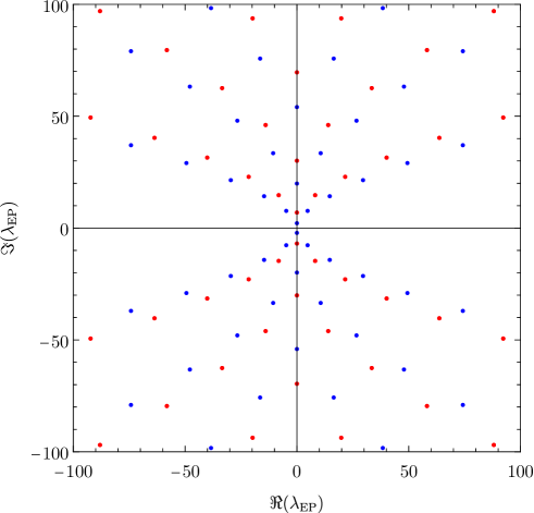
Figure 3: EPS for the Mathieu equation with period $\pi$ for even (blue circles) and odd (red circles) functions

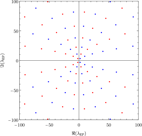
Figure 4: EPS for the Mathieu equation with period $2\pi$ for even (blue circles) and odd (red circles) functions

Since in the four cases we have tridiagonal matrices, we resort to the recurrence relation for the determinants $D_{N}$ discussed in B. Thus, the problem reduces to obtaining the roots of a polynomial $F_{N}(\lambda)=Disc_{E}(D_{N}(E,\lambda))$ of degree $N(N+1)$. Present results are shown in figures 3 and 4. In the case of period $\pi$ the distribution of EPS for each parity symmetry (even and odd) exhibit the characteristic symmetry with respect to both axes. However, in the case of those of period $2\pi$ the even functions exhibit EPS $\lambda_{EP}$ and $\lambda_{EP}^{\ast}$ while the odd functions exhibit the remaining ones $-\lambda_{EP}$ and $-\lambda_{EP}^{\ast}$. The reason is that for period $\pi$ $D_{N}^{e,o}(E,-\lambda)=D_{N}^{e,o}(E,\lambda)$ while for period $2\pi$ $D_{N}^{e}(E,-\lambda)=D_{N}^{o}(E,\lambda)$, where the superscripts $e$ and $o$ stand for even and odd parity, respectively.

Present results agree with those of Blanch and Clemm[4] in the whole $\lambda$ plane and the ones obtained by Fernández and Garcia[11] on the imaginary axis. Both appear to be the most accurate EPS available in the literature.

5 Polar rigid rotor in a uniform electric field

In this section we consider a rigid rotor with dipole moment $\mu$ in a uniform electric field of intensity $F$. The kinetic energy of the Hamiltonian operator is $\mathcal{L}^{2}/(2I)$, where, $\mathcal{L}^{2}$ is the square of the angular momentum and $I$ is the moment of inertia. The interaction with the field is $-\mu F\cos\theta$, where $\theta$ is the angle between the dipole moment and the field direction. This model has proved useful for the analysis of the rotational Stark effect in linear polar molecules[27]. The Schrödinger equation can be written in dimensionless form as $H(\lambda)\psi=\epsilon(\lambda)\psi$, where

$$H(\lambda)=H_{0}+\lambda H^{\prime}=L^{2}-\lambda\cos\theta,$$ (12)

$L^{2}=\mathcal{L}^{2}/\hbar^{2}$, $\lambda=2I\mu F/\hbar^{2}$ and $\epsilon=2IE/\hbar^{2}$. As in the preceding example we have $\left\|H^{\prime}\Phi\right\|\leq\left\|\Phi\right\|$ and because of the transformation $U^{\dagger}\theta U=\theta+\pi\Rightarrow U^{\dagger}H(\lambda)U=H(-\lambda)$ we expect a distribution of EPS that is symmetric with respect to both axes in the complex $\lambda$ plane.

In order to apply present approach we resort to a matrix representation of the Hamiltonian operator in the basis set of eigenfunctions of $L^{2}$ and $L_{z}$

$$L^{2}\left|l,m\right\rangle = l(l+1)\left|l,m\right\rangle,\;l=0,1,\ldots,$$

$$L_{z}\left|l,m\right\rangle = m\left|l,m\right\rangle,\;m=0,\pm 1,\ldots,\pm l.$$ (13)

It is well known that the coefficients $c_{i}$ of the expansion

$$\psi=\sum_{i=0}^{\infty}c_{i}\left|M+i,m\right\rangle,\;M=|m|,$$ (14)

satisfy a three-term recurrence relation like those discussed in the B with[27, 3]

$$A_{i}=-\lambda\left[\frac{i(i+2M)}{4(i+M)^{2}-1}\right]^{1/2},\;B_{i}=(i+M)(i+M+1)-\epsilon.$$ (15)

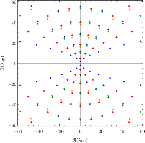
Figure 5: EPS for the rigid rotor in an electric field for the states with $M=0$ (blue circles) $M=1$ (red diamonds) $M=2$ (green triangles) and $M=3$ (orange stars)

The calculation of the EPS $\lambda_{EP}$ from the determinants $D_{N}(\epsilon,\lambda)=0$ (see B) is straightforward and some results are shown in figure 5 for $M=0,1,2,3$. It is worth noticing that the EPS for $M=0$ are close to those for $M=2$ while the EPS for $M=1$ are close to those for $M=3$. Notice that the distribution of EPS exhibits the symmetry with respect to both axes mentioned above.

6 Polar symmetric top in a uniform electric field

The rotational Stark effect in a symmetric-top molecule is commonly studied by means of the model Hamiltonian[27, 28, 29]

$$H = -\frac{\hbar^{2}}{2I_{B}}\left[\frac{1}{\sin\theta}\frac{\partial}{\partial\theta}\sin\theta\frac{\partial}{\partial\theta}+\frac{1}{\sin^{2}\theta}\frac{\partial^{2}}{\partial\phi^{2}}+\left(\frac{\cos^{2}\theta}{\sin^{2}\theta}+\frac{I_{B}}{I_{C}}\right)\frac{\partial^{2}}{\partial\chi^{2}}-\frac{2\cos\theta}{\sin^{2}\theta}\frac{\partial^{2}}{\partial\phi\partial\chi}\right]$$ (16)

$$-\mu F\cos\theta,$$

where $I_{C}$ is the moment of inertia about the symmetry axis, $I_{B}$ is the other moment of inertia, $\phi$, $\theta$ and $\chi$ are the Euler angles, $\mu$ is the dipole moment of the molecule and $F$ is the intensity of the uniform electric field. Clearly, $\theta$ is the angle between the dipole moment and the field direction.

The Schrödinger equation $H\psi=E\psi$ is separable if we write $\psi(\theta,\phi,\chi)=\Theta(\theta)e^{iM\phi}e^{iK\chi}$, where $M,K=0,\pm 1,\pm 2,\ldots$ are the two rotational quantum numbers that remain when the field is applied. The resulting eigenvalue equation in dimensionless form is

$$\left(\frac{1}{\sin\theta}\frac{d}{d\theta}\sin\theta\frac{d}{d\theta}-\frac{M^{2}}{\sin^{2}\theta}-\frac{\cos^{2}\theta}{\sin^{2}\theta}K^{2}+\frac{2\cos\theta}{\sin^{2}\theta}KM-\lambda\cos\theta+\epsilon\right)\Theta=0,$$

$$\epsilon=\frac{2I_{B}}{\hbar^{2}}E-\frac{I_{B}}{I_{C}}K^{2},\;\lambda=\frac{2I_{B}}{\hbar^{2}}\mu F.$$ (17)

If we write $H(\lambda)=H_{0}+\lambda H^{\prime}$ then we realize that $\left\|H^{\prime}\Phi\right\|\leq\left\|\Phi\right\|$ as in the two preceding examples. Besides, the transformation used in the case of the rigid rotor leads to $U^{\dagger}H(\lambda)U=H(-\lambda)$ and once again we expect a distribution of EPS that is symmetric with respect to both axes.

In this case we obtain a suitable matrix representation of the Hamiltonian in the basis set of eigenvectors $\left|J,M,K\right\rangle$ of the free symmetric top ($\lambda=0$). The coefficients $c_{i}$ of the expansion

$$\psi=\sum_{i=0}^{\infty}c_{i}\left|J_{0}+i,M,K\right\rangle,\;J_{0}=\max(|M|,|K|),$$ (18)

satisfy a three-term recurrence relation with[27, 28, 29]

$$B_{i} = \left(J_{0}+i\right)\left(J_{0}+i+1\right)-\lambda\frac{MK}{\left(J_{0}+i\right)\left(J_{0}+i+1\right)}-\epsilon,$$

$$A_{i} = -\lambda\frac{\sqrt{\left[\left(J_{0}+i\right)^{2}-K^{2}\right]\left[\left(J_{0}+i\right)^{2}-M^{2}\right]}}{\left(J_{0}+i\right)\sqrt{4\left(J_{0}+i\right)^{2}-1}}.$$ (19)

Therefore, we can obtain the EPS from the secular determinants $D_{N}(\epsilon,\lambda)=0$ for a sufficiently large dimension $N$ (see B).

The distribution of the EPS can be predicted from the set of equalities

$$D_{N}(\epsilon,M,K,\lambda)=D_{N}(\epsilon,K,M,\lambda)=D_{N}(\epsilon,-M,-K,\lambda)=D_{N}(\epsilon,-K,-M,\lambda)=$$

$$D_{N}(\epsilon,-M,K,-\lambda)=D_{N}(\epsilon,K,-M,-\lambda)=D_{N}(\epsilon,M,-K,-\lambda)=$$

$$D_{N}(\epsilon,-K,M,-\lambda).$$ (20)

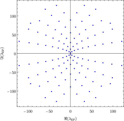
Figure 6: EPS for the polar symmetric top in a uniform electric field for $M=0$ and $K=0$

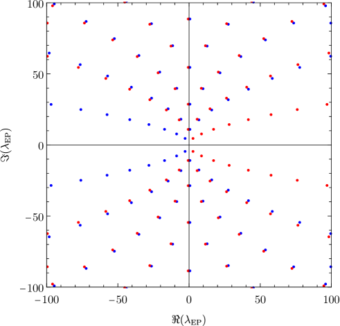
Figure 7: EPS for the polar symmetric top in a uniform electric field for $(M=1,K=1)$ (blue circles) and $(M=1,K=-1)$ (red circles)

Figure 6 shows that the distribution of EPS for $M=K=0$ is symmetric with respect to both axes. On the other hand, Figure 7 shows that the distribution of EPS for either $MK=1$ or $MK=-1$ is symmetric with respect to the real axis but the union of both sets is symmetric with respect to both axes.

Present results are considerably more accurate than those obtained earlier for this model[7, 13].

7 Conclusions

In this paper we have shown that the discriminant is an extremely useful tool for the location of EPS in the eigenvalues of parameter-dependent Hamiltonian operators. In all the previous studies that we are aware of, the approach was applied to operators on finite Hilbert spaces with matrix representations of finite dimension that lead to characteristic polynomials of finite degree[17, 18, 19, 20, 21, 22, 23, 24, 25, 26]. Here, on the other hand, the Hilbert spaces have infinite dimension so that the truncated $N$-dimensional matrix representations, as well as the corresponding characteristic polynomials are approximate. However, the location approach based on the discriminant applies successfully producing sequences of roots that converge towards the actual EPS as $N$ increases. Any spurious root is easily identified because it does not form part of a convergent sequence.

All the examples chosen in the present study are of mathematical or physical interest. Our results for the Mathieu equation agree with the most extended and accurate ones available in the literature[4] and those for the Stark effects in the rigid rotor and symmetric top are either more extended or more accurate than the ones published previously[3, 7, 11, 12, 13].

Appendix A Resultant and discriminant

In this section we summarize those properties of the discriminant of a polynomial that are relevant for present paper. The resultant of two polynomials

$$f(x) = \sum_{j=0}^{m}a_{m-j}x^{j},$$

$$g(x) = \sum_{j=0}^{n}b_{m-j}x^{j},$$ (21)

is given by the determinant

$$Res_{x}(f,g)=\left|\begin{array}[]{cccccccc}a_{0}&0&\cdots&0&b_{0}&0&\cdots&0\\ a_{1}&a_{0}&\cdots&0&b_{1}&b_{0}&\cdots&0\\ a_{2}&a_{1}&\ddots&0&b_{2}&b_{1}&\ddots&\vdots\\ \vdots&\vdots&\ddots&a_{0}&\vdots&\vdots&\ddots&b_{0}\\ a_{m}&a_{m-1}&\cdots&\vdots&b_{n}&b_{n-1}&\cdots&\vdots\\ 0&a_{m}&\ddots&\vdots&0&b_{n}&\ddots&\vdots\\ \vdots&\vdots&\ddots&a_{m-1}&\vdots&\vdots&\ddots&b_{n-1}\\ 0&0&\cdots&a_{m}&0&0&\cdots&b_{n}\end{array}\right|.$$ (22)

It can be proved that

$$Res_{x}(f,g)=a_{0}^{m}b_{0}^{n}\prod_{i=1}^{m}\prod_{j=1}^{n}\left(\xi_{i}-\mu_{j}\right),$$ (23)

where $\xi_{i}$ and $\mu_{j}$ are the roots of the polynomials $f$ and $g$, respectively. The discriminant of $f(x)$ is defined as

$$Disc_{x}(f)=\frac{(-1)^{m(m-1)/2}}{a_{m}}Res_{x}(f,f^{\prime}),$$ (24)

and in this case we have

$$Disc_{x}(f)=a^{2m-2}\prod_{i<j}\left(\xi_{i}-\xi_{j}\right)^{2}.$$ (25)

Suppose that the nonlinear equation $Q(E,\lambda)=0$ gives us the eigenvalues $E(\lambda)$ of a quantum-mechanical system. If this equation is a polynomial function of $E$, then the roots of $F(\lambda)=Disc_{E}(Q(E,\lambda))$ are the exceptional points $\lambda_{EP}$ in the complex $\lambda$ plane where at least two eigenvalues coalesce. We appreciate that the advantage of resorting to the discriminant is that we only have to search for the roots of a nonlinear function of just one variable. In all the examples studied here the nonlinear equation $Q(E,\lambda)$ is a polynomial function of both $E$ and $\lambda$ so that $F(\lambda)$ is a polynomial function of $\lambda$ (see B, and the examples). Consequently, the calculation is particularly simple because there are efficient algorithms for finding the roots of polynomials. Besides, most computer-algebra software enable one to obtain analytical expressions for $F(\lambda)$ because the discriminant is given by a determinant. Thus, the only numerical step of the calculation reduces to finding the roots of the polynomial $F(\lambda)$.

As an illustrative example we consider a trivial toy problem that we deem to be quite interesting: the Hamiltonian operator in matrix form

$$\mathbf{H}(\beta,\lambda)=\left(\begin{array}[]{ccc}3-\lambda&\beta&0\\ \beta&2&\beta\\ 0&\beta&1+\lambda\end{array}\right).$$ (26)

When $\beta=0$ the three eigenvalues cross at $\lambda=1$ and the three eigenvectors are degenerate (they are obviously linearly independent). However, when $\beta\neq 0$ the eigenvalues do not cross for real values of $\lambda$ and exhibit avoided crossings as shown in Figure 8 for $\beta=0.1$.

The characteristic polynomial is

$$Q(E,\lambda)=\frac{\left(2-E\right)\left(50E^{2}-200E-50\lambda^{2}+100\lambda+149\right)}{50},$$ (27)

so that

$$Disc_{E}(Q(E,\lambda))=\frac{\left(50\lambda^{2}-100\lambda+51\right)^{3}}{31250}.$$ (28)

We appreciate that the three eigenvalues coalesce at any of the two EPS $\lambda_{EP}=1+\sqrt{2}i/10$ and $\lambda_{EP}^{\ast}$ that are branch points of order two. The structure of the avoided crossings in this toy model is similar to that of the modified Lipkin model for $N=3$[21].

At $\lambda_{EP}$ (a similar analysis can be carried out at $\lambda_{EP}^{\ast}$) the matrix $\mathbf{H}$ has only one eigenvalue $E\left(\lambda_{EP}\right)=2$ and only one eigenvector

$$\mathbf{v}_{1}=\frac{1}{2}\left(\begin{array}[]{c}-i\\ \sqrt{2}\\ i\end{array}\right),$$ (29)

so that $\mathbf{H}$ is defective. By means of the Jordan chain

$$\left(\mathbf{H}-2\mathbf{I}_{3}\right)\mathbf{v}_{2} = \mathbf{v}_{1},$$

$$\left(\mathbf{H}-2\mathbf{I}_{3}\right)\mathbf{v}_{3} = \mathbf{v}_{2},$$ (30)

where $\mathbf{I}_{3}$ is the $3\times 3$ identity matrix, we obtain two additional vectors $\mathbf{v}_{2}$ and $\mathbf{v}_{3}$ and the matrix

$$\mathbf{U}=\left(\begin{array}[]{ccc}\mathbf{v}_{1}&\mathbf{v}_{2}&\mathbf{v}_{3}\end{array}\right)=\left(\begin{array}[]{ccc}-i/2&5\sqrt{2}&0\\ 1/\sqrt{2}&5i&50\sqrt{2}\\ i/2&0&50i\end{array}\right),$$ (31)

that converts $\mathbf{H}$ into a Jordan canonical form

$$\mathbf{U}^{-1}\mathbf{HU}=\left(\begin{array}[]{ccc}2&1&0\\ 0&2&1\\ 0&0&2\end{array}\right).$$ (32)

In this simple case we can easily obtain the EPS directly from the eigenvalues but in most nontrivial problems the use of the discriminant leads to far simpler expressions.

Appendix B Three-term recurrence relations

Suppose that there is an orthonormal basis set $\left\{\left|i\right\rangle,i=0,1,\ldots\right\}$ such that

$$H\left|i\right\rangle=H_{i,i-1}\left|i-1\right\rangle+H_{i,i}\left|i\right\rangle+H_{i,i+1}\left|i+1\right\rangle,$$ (33)

where $H_{i,j}=H_{i,j}^{\ast}=H_{j,i}$. Therefore, if we expand

$$\psi=\sum_{i}c_{i}\left|i\right\rangle,$$

the Schrödinger equation $H\psi=E\psi$ becomes a three-term recurrence relation for the coefficients $c_{j}$:

$$A_{i}c_{i-1}+B_{i}c_{i}+A_{i+1}c_{i+1} = 0,\;A_{i}=H_{i-1,i},\;B_{i}=H_{ii}-E,$$ (34)

$$i=0,1,2\ldots,\;c_{-1}=0.$$

One commonly obtains approximate energies by means of the truncation condition $c_{j}=0$, $j>N$, so that the roots of the characteristic polynomial given by the secular determinant

$$D_{N}=\left|\begin{array}[]{cccccc}B_{0}&A_{1}&0&\cdots&\cdots&0\\ A_{1}&B_{1}&A_{2}&0&\cdots&0\\ \vdots&\vdots&\vdots&\ddots&\cdots&\vdots\\ 0&0&\cdots&A_{N-1}&B_{N-1}&A_{N}\\ 0&0&\cdots&0&A_{N}&B_{N}\end{array}\right|,$$ (35)

converge from above toward the actual energies of the physical problem when $N\rightarrow\infty$. These determinants can be efficiently generated by means of the three-term recurrence relation[28, 29, 3]

$$D_{N}=B_{N}D_{N-1}-A_{N}^{2}D_{N-2},\;N=0,1,\ldots,$$ (36)

with the initial conditions $D_{-1}=1$, $D_{j}=0$ for $j<-1$. Notice that the dimension of the determinant $D_{N}$ is $N+1$.

Bibliography

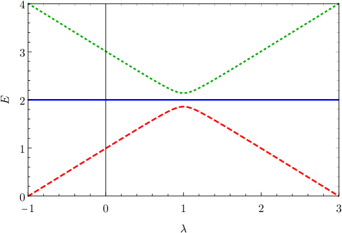
Figure 8: Avoided crossings for the three-level model

Bibliography

- [1] Reed M and Simon B 1978 Methods of Modern Mathematical Physics, IV. Analysis of Operators (Academic, New York).
- [2] Simon B 1982 Int. J. Quantum Chem. 21 3.
- [3] Fernández F M 2001 Introduction to Perturbation Theory in Quantum Mechanics (CRC Press, Boca Raton).
- [4] Blanch G and Clemm D S 1969 Math. Comput. 23 97.
- [5] Hunter C 1981 North-Holland Math. Studies 55 233.
- [6] Hunter C and Guerrieri B 1981 Studies Appl. Math. 64 113.
- [7] Fernández F M, Arteca G A, and Castro E A 1987 J. Math. Phys. 28 323.
- [8] Volkmer H 1998 Math. Nachr. 192 239.
- [9] Shivakumar P N and Xue J 1999 J. Comput. Appl. Math 107 111.
- [10] Ziener C H, Rückl M, Kampf T, Bauer W R, and Schlemmer H P 2012 J. Comput. Appl. Math 236 4513.
- [11] Fernández F M and Garcia J 2014 Appl. Math. Comput. 247 141.
- [12] Fernández F M and Castro E A 1985 Phys. Lett. A 107 215.
- [13] Mesón M, A. M S, Fernández F M, and Castro E A 1987 Phys. Lett. A 124 4.
- [14] Sylvester J J 1851 The London, Edinburgh, and Dublin Philosophical Magazine and Journal of Science. Series 4 2 391.
- [15] Griffiths H B 1981 Am. Math. Month. 88 328.
- [16] Basu S, Pollack R, and Roy M-F 2003 Algorithms in Real Algebraic Geometry (Springer-Verlag, Berlin).
- [17] Stepanov V V and Müller G 1998 Phys. Rev. E 58 5720.
- [18] Heiss W D and Steeb W-H 1991 J. Math. Phys. 32 3003.
- [19] Davis T J 2002 Eur. Phys. J. D 18 27.
- [20] Freund I 2004 J. Opt. A 6 S229.
- [21] Heiss W D, Scholtz F G, and Geyer H B 2005 J. Phys. A 38 1843.
- [22] Bhattacharya M and Raman C 2006 Phys. Rev. Lett. 97 140405.
- [23] Bhattacharya M 2007 Am. J. Phys. 75 942.
- [24] Bhattacharya M and Raman C 2007 Phys. Rev. A. 75 033405.
- [25] Bhattacharya M and Raman C 2007 Phys. Rev. A 75 033406.
- [26] Kotvytskiy A T and Bronza S D 2016 Odessa Astron. Pub. 29 31.
- [27] Townes C H and Schawlow A L 1955 Microwave Spectroscopy (McGraw-Hill, New York).
- [28] Shirley J H 1963 J. Chem. Phys. 38 2896.
- [29] Hajnal J V and Opat G I 1991 J. Phys. E 24 2799.