Transition between Amplified Spontaneous Emission and Superfluorescence in a longitudinally pumped medium by an X-ray free electron laser pulse

Abstract

The transition from the amplification of spontaneous emission to superfluorescence in a three-level and swept-gain medium excited by an X-ray free electron laser pulse is theoretically investigated. Given the specific time scale of X-ray free electron laser pulse, we investigate the swept pumping process in detail and our results show that the temporal structure of an X-ray free electron laser pulse plays a more critical role than its peak intensity does for producing population inversion. The typical watershed of two radiant regions depends on the optical depth of the gain medium for a given coherence time, namely, particle number density and the medium length are equally important. However, we find that medium length plays more important role than particle density does for making the forward-backward asymmetry. The transient gain length and the total medium length are identified as two important factors to observe length induced backward transition. The present results suggest an application of parametric controls over a single-pass-amplified light source.

I Introduction

Absorption, stimulated emission and spontaneous emission of photons are three fundamental processes of light-matter interaction. However, a collection of excited atoms emits light differently from what a single atom does. One type of such collective light emission was first theoretically studied in Dicke’s pioneering and seminal work of superfluorescence (SF) Dicke (1954). While in free space a wavepacket of photons isotropically emitted by a single atom behaves like it is exponentially decaying with a duration of an excited state lifetime, SF from multiple atoms with particle density $n$ for a given sample length $L$ acts as a directional light burst characterized by its peak intensity, duration and time delay, which are proportional to $n^{2}$, $n^{-1}$ and $n^{-1}$, respectively Polder et al. (1979); Gross and Haroche (1982). SF was first experimentally realized in room-temperature HF gas Skribanowitz et al. (1973), and subsequently observed in, e.g., Sodium Gross et al. (1976), Cesium Gibbs et al. (1977), Rubidium atoms Paradis et al. (2008), solid-state KCl$:$O${}_{2}^{-}$ Florian et al. (1984); Malcuit et al. (1987) and in plasma Dreher et al. (2004); Noe II et al. (2012). More recently, the development of a free electron laser (FEL) Deacon et al. (1977) has lead to further advancements, such as the observation of EUV-FEL-induced SF in Helium gas Nagasono et al. (2011), XUV-FEL-induced SF in Xenon gas Mercadier et al. (2019) and FEL superfluorescence Watanabe et al. (2007). Apart from typical three-level-$\Lambda$ type atomic systems Gibbs et al. (1977); Nagasono et al. (2011); Cui et al. (2012, 2013); Cui and Macovei (2017), a V-type one Keitel et al. (1992); Kozlov et al. (1999) has also been theoretically investigated.

Another kind of collective emission is the so-called amplification of spontaneous emission (ASE) Gross and Haroche (1982); Pert (1994); Rohringer et al. (2012); Weninger and Rohringer (2014); Yoneda et al. (2015), namely, radiation due to spontaneous emission from a single emitter is amplified when it propagates through an excited sample. While ASE is also directional due to the geometry of the inverted medium, the time structure of ASE is quite distinct from that of SF, e.g., the peak intensity does not behave as $n^{2}$ Schuurmans and Polder (1979); Malcuit et al. (1987). Utilizing the ASE mechanism, an atomic inner shell laser pumped by an X-ray Free Electron Laser (XFEL) has recently been achieved Rohringer et al. (2012); Weninger and Rohringer (2014); Yoneda et al. (2015). While this achievement Rohringer et al. (2012); Yoneda et al. (2015) has become milestone within the field of X-Ray quantum optics Shvyd’ko et al. (1996); Röhlsberger et al. (2010); Liao et al. (2011); Röhlsberger et al. (2012); Liao et al. (2012); Adams et al. (2013); Liao et al. (2013); Vagizov et al. (2014); Liao and Pálffy (2014); Heeg et al. (2015); Liao and Ahrens (2015); Heeg et al. (2017); Wang and Liao (2018), XFEL-induced SF has never been studied. Moreover, SF and ASE are independently investigated in most works with only few examples touching on both Bonifacio et al. (1971a, b); Okada et al. (1978); Brechignac and Cahuzac (1981); Malcuit et al. (1987); Rai and Bowden (1992). Studying XFEL-pumped SF, as well as the transition from ASE to SF using XFEL, is therefore interesting and timely.

Most theoretical studies of ASE or SF rely on three assumptions: (i) a completely inverted medium as the initial condition Haake et al. (1979a, b); Schuurmans and Polder (1979); Gross and Haroche (1982), (ii) a swept-gain amplifier excited by an oversimplified $\delta$-function pulse Arecchi and Courtens (1970); Bonifacio et al. (1975); Hopf and Meystre (1975), and (iii) only forward emission of light Arecchi and Courtens (1970); Bonifacio et al. (1975); Haake et al. (1979a, b); Schuurmans and Polder (1979); Rai and Bowden (1992); Weninger and Rohringer (2014). In view that XFEL pulse duration may be greater than the excited state lifetime Rohringer et al. (2012); Yoneda et al. (2015), the assumption (ii) Arecchi and Courtens (1970); Bonifacio et al. (1975); Hopf and Meystre (1975) is unrealistic. One therefore has to carefully deal with the pumping process. We use (a) a swept-gain amplifier excited by a short XFEL pumping pulse with a duration of a few tens femtosecond Eur , and (b) a set of equations describing both the forward and backward emission. Our detailed study of this issue identifies the mechanism breaking the forward and backward symmetry and demonstrates that the time structure of the pumping pulse is highly critical for producing population inversion. Typically, the ASE-SF transition depends only on $\tau_{2}\gg\sqrt{\tau_{R}\tau_{D}}$ or $\tau_{R}\ll\tau_{2}\ll\sqrt{\tau_{R}\tau_{D}}$, where $\tau_{2}$ is the coherence time of the transition, $\tau_{R}$ the characteristic duration of SF and $\tau_{D}$ the SF delay time Friedberg and Hartmann (1976); Schuurmans and Polder (1979); Malcuit et al. (1987). The definition of $\tau_{R}$ and $\tau_{D}$ shows that the length of a medium and particle density are equally important for ASE-SF transition. However, our study on the pumping process shows that the choice of medium length plays a more important role than particle density does for observing backward emission, namely, medium length induced ASE-SF transition can happen to the backward emission. Apart from the typical averaged temporal behavior of emitted light pulses, we show that both the averaged spectrum and the histogram of emitted photon number manifest the ASE-SF transition. Our results therefore give useful hints for quantifying the XFEL-pumped light source and demonstrate in what parameter region the transition may occur. The present results suggest an application of modifying the properties of a single-pass light source Rohringer et al. (2012); Weninger and Rohringer (2014); Yoneda et al. (2015); Gunst et al. (2014); ten Brinke et al. (2013); Zhang and Svidzinsky (2013) via the transition between ASE and SF induced by the change of optical depth of the gain medium or by the variety of a pumping pulse.

This paper is organized as follows. In Sec. II, we describe our system and theoretical model using the Maxwell-Bloch equation. In Sec. III, we present our analysis of the production of population inversion. In Sec. IV, we numerically solve these coupled equations and discuss the transition between ASE and SF. In Sec. V, the length effects for forward-backward asymmetry are discussed. In Sec. VI, we demonstrate the transition between ASE and SF induced by the variety of pumping laser parameters. A summary is present in Sec. VII.

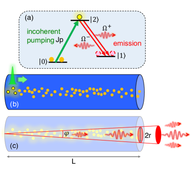
Figure 1: (Color online) (a) three-level $\Lambda$-type scheme. Transition $|0\rangle\rightarrow|2\rangle$ is incoherently pumped by a short pumping laser pulse $J_{p}$ (green upward arrow). Atoms promoted to state $|2\rangle$ subsequently decay and become state $|1\rangle$. Atoms that undergo the transition $|2\rangle\rightarrow|1\rangle$ emit photons (red downward arrows) in the forward and backward direction with equal probability. (b) atoms in state $|0\rangle$ (orange dots) are initially prepared in a gas cell. When a pumping pulse (green filled Gaussian pulse) is travelling through, atoms are promoted to state $|2\rangle$ (yellow filled circles) in a region defined by the spot size and path of the pumping pulse $J_{p}$. (c) $\varphi$ in Eq. (16) represents the solid angle within which the emitted photons due to transition $|2\rangle\rightarrow|1\rangle$ get amplified in the forward direction. $\varphi$ is determined by the length $L$ and the transverse radius $r$ of the medium.

II Model

Table 1: The notation used throughout the text. The indices $i,j\in\left\{0,1,2\right\}$ denote the three states showed in Fig. 1(a).

Notation	Explanation
$c$	Speed of light in vacuum.
$\varepsilon_{0}$	Vacuum permittivity.
$\Omega^{+\left(-\right)}$	Slowly varying Rabi frequency of forward (backward)
	emission from $|2\rangle\rightarrow|1\rangle$ transition.
$I_{\mathrm{avg}}^{\pm}\left(t\right)$	Average temporal intensity of $\Omega^{\pm}$.
$S_{\mathrm{avg}}^{\pm}\left(\omega\right)$	Average spectral intensity of $\Omega^{\pm}$.
$F^{+\left(-\right)}$	Gaussian white noise and the source term of
	forward (backward) emission.
$\delta\left(\tau-t\right)$	Dirac delta function.
$\varphi$	Solid angle for collecting emitted photons in the
	forward and backward direction.
$\tau_{2}$	Lifetime of state $|2\rangle$.
$\Gamma$	$=1/\tau_{2}$, spontaneous decay rate of state $|2\rangle$.
$\lambda$	Wavelength of $|1\rangle\rightarrow|2\rangle$ transition.
$\rho_{ii}$	$=B_{i}B_{i}^{*}$ for state vector $\sum_{i=0}^{2}B_{i}|i\rangle$,
	the diagonal density matrix element.
$\rho_{21}^{+\left(-\right)}$	Forward (backward) component of the coherence
	$B_{2}B_{1}^{*}$ for state vector $\sum_{i=0}^{2}B_{i}|i\rangle$.
$\delta_{ij}$	Kronecker delta symbol.
$n$	Number density of particles.
$\sigma$	Absorption cross section of transition $|0\rangle\rightarrow|2\rangle$.
$\sigma_{r}$	$=3\lambda^{2}/\left(2\pi\right)$, resonant cross section of transition $|1\rangle\rightarrow|2\rangle$.
$L$	Length of the medium.
$L_{g}$	$=c\tau_{p}/2$, transient gain length.
$\alpha$	$=n\sigma_{r}L$, optical depth of $|1\rangle\rightarrow|2\rangle$ transition.
$\eta$	$=\Gamma\alpha/\left(2L\right)$, the light-matter coupling constant.
$\omega$	Angular frequency of $|1\rangle\rightarrow|2\rangle$ transition.
$d$	Transition dipole moment of $|1\rangle\rightarrow|2\rangle$ transition.
$J_{p}$	Intensity of pumping light pulse.
$\tau_{p}$	Pulse duration of pumping laser pulse.
$r$	Radius of $J_{p}$ laser spot which determines the transverse
	radius of the gain medium.
$\tau_{i}$	Peak position of incident pumping laser pulse.
$n_{p}$	Number of photons per pumping laser pulse.
$n_{e}$	Number of photons emitted by $|2\rangle\rightarrow|1\rangle$ transition.
$Q$	A parameter utilized to adjust the amplitude of $J_{p}$ in Fig. 3.
$\tau_{R}$	Characteristic duration of superfluorescence Friedberg and Hartmann (1976); Schuurmans and Polder (1979); Malcuit et al. (1987).
$\tau_{D}$	Delay time of superfluorescence Friedberg and Hartmann (1976); Schuurmans and Polder (1979); Malcuit et al. (1987).

Figure 1(a) illustrates our three-level $\Lambda$-type system. A pumping light pulse $J_{p}$ incoherently drives transition $|0\rangle\rightarrow|2\rangle$, e.g., ionization, when propagating through a one dimensional gas medium as demonstrated in Fig 1(b). The orange dots and yellow filled circles, respectively, denote particles in state $|0\rangle$ and $|2\rangle$. For simplicity, promoted particles in state $|2\rangle$ subsequently experience only one decay channel $|2\rangle\rightarrow|1\rangle$ and emit photons in both the forward and backward direction with equal probability (red wiggled arrows). Red dashed and filled circles represent decayed particles in state $|1\rangle$, and the green Gaussian pulse depicts $J_{p}$. We numerically analyse the emission behaviour for different parameters of the medium and that of $J_{p}$. The Maxwell-Bloch equation Arecchi and Courtens (1970); MacGillivray and Feld (1976); Polder et al. (1979); Schuurmans and Polder (1979); Yuan and Svidzinsky (2012); Weninger and Rohringer (2014) with forward-backward decomposition Lin et al. (2009); Liao and Pálffy (2014); Su et al. (2016) is used to describe the dynamics including the incoherent and longitudinal pumping:

$$\partial_{t}\rho_{00} = -\sigma J_{p}\rho_{00},$$ (1)

$$\partial_{t}\rho_{11} = \Gamma\rho_{22}-\frac{i}{2}\left(\Omega^{+}\rho_{21}^{+*}-\Omega^{+*}\rho_{21}^{+}\right)$$ (2)

$$- \frac{i}{2}\left(\Omega^{-}\rho_{21}^{-*}-\Omega^{-*}\rho_{21}^{-}\right),$$

$$\partial_{t}\rho_{22} = \sigma J_{p}\rho_{00}-\Gamma\rho_{22}+\frac{i}{2}\left(\Omega^{+}\rho_{21}^{+*}-\Omega^{+*}\rho_{21}^{+}\right)$$ (3)

$$+ \frac{i}{2}\left(\Omega^{-}\rho_{21}^{-*}-\Omega^{-*}\rho_{21}^{-}\right),$$

$$\partial_{t}\rho_{21}^{+} = -\frac{\Gamma}{2}\rho_{21}^{+}-\frac{i}{2}\left(\rho_{22}-\rho_{11}\right)\Omega^{+}+F^{+},$$ (4)

$$\partial_{t}\rho_{21}^{-} = -\frac{\Gamma}{2}\rho_{21}^{-}-\frac{i}{2}\left(\rho_{22}-\rho_{11}\right)\Omega^{-}+F^{-},$$ (5)

$$\frac{1}{c}\partial_{t}J_{p} + \partial_{z}J_{p}=-n\rho_{00}\sigma J_{p},$$ (6)

$$\frac{1}{c}\partial_{t}\Omega^{+} + \partial_{z}\Omega^{+}=i\eta\rho_{21}^{+},$$ (7)

$$\frac{1}{c}\partial_{t}\Omega^{-} - \partial_{z}\Omega^{-}=i\eta\rho_{21}^{-};$$ (8)

together with initial and boundary conditions

$$\rho_{ij}\left(0,z\right) = \delta_{i0}\delta_{j0},$$ (9)

$$\rho_{21}^{\pm}\left(0,z\right) = 0,$$ (10)

$$J_{p}\left(0,z\right) = 0,$$ (11)

$$\Omega^{\pm}\left(0,z\right) = 0,$$ (12)

$$J_{p}\left(t,0\right) = \frac{n_{p}}{\pi^{3/2}r^{2}\tau_{p}}Exp\left[-\left(\frac{t-\tau_{i}}{\tau_{p}}\right)^{2}\right],$$ (13)

$$\Omega^{+}\left(t,0\right) = 0,$$ (14)

$$\Omega^{-}\left(t,L\right) = 0.$$ (15)

The emission process starts from Gaussian white noise $F^{\pm}$ obeying the delta correlation function Weninger and Rohringer (2014); Haake et al. (1979a, b); Polder et al. (1979); Gross and Haroche (1982)

$$\langle F^{\pm}(\tau)F^{\pm*}(t)\rangle=\frac{\varphi\rho_{22}\Gamma^{2}\omega^{2}}{24n\pi^{2}c^{3}}\delta(\tau-t),$$ (16)

where

$$\varphi=\int_{0}^{2\pi}d\phi\int_{0}^{\tan^{-1}\left(\frac{r}{L}\right)}\sin\theta d\theta=2\pi-\frac{2\pi}{\sqrt{1+\frac{r^{2}}{L^{2}}}}.$$

Based on an experimental fact Vrehen and der Weduwe (1981) and Gross and Haroche (1982), we use

$$\langle F^{\pm}(\tau)F^{\mp*}(t)\rangle=0.$$

All notation in above equations is listed and explained in Table 1, and the quantities used for each figure in what follows are listed in Table 2. Fig. 1(c) illustrates the solid angle $\varphi$ used in Eq. (16) Arecchi and Courtens (1970). $\varphi$ is determined by the geometry of the gain medium, i.e., an ensemble of atoms longitudinally pumped to state $|2\rangle$ by a $J_{p}$ pulse. $\varphi$ is therefore affected by the length of the medium $L$ and the radius $r$ of the $J_{p}$ laser spot. Those photons randomly emitted within $\varphi$ will interact with most of excited atoms and lead to, e.g., stimulated emission. The value from the complete form of $\varphi$ is used in all of our numerical calculations, and $\varphi$ can be simplified to an intuitive value $\pi r^{2}/L^{2}$ for typical theoretical studies since $r\ll L$ is implicitly assumed in the 1D model. However, in realistic systems, diffraction (3D effects) can limit the effective solid angle to $\lambda^{2}/r^{2}$, and can change the simulation results. This problem is associated with Fresnel number $\mathbf{F}$ Gross and Haroche (1982) and will be discussed in Sec. IV. The ensemble average of temporal intensity $\langle I^{\pm}\left(t\right)\rangle$ is defined as

$$\langle I^{+}\left(t\right)\rangle = \frac{1}{N_{e}}\sum_{n=1}^{N_{e}}|\Omega_{n}^{+}\left(t,L\right)|^{2},$$

$$\langle I^{-}\left(t\right)\rangle = \frac{1}{N_{e}}\sum_{n=1}^{N_{e}}|\Omega_{n}^{-}\left(t,0\right)|^{2}.$$ (17)

and the ensemble average of spectral intensity $\langle S^{\pm}\left(\omega\right)\rangle$ is defined as

$$\langle S^{+}\left(\omega\right)\rangle = \frac{1}{N_{e}}\sum_{n=1}^{N_{e}}|\int_{-\infty}^{\infty}\Omega_{n}^{+}\left(t,L\right)e^{i\omega t}dt|^{2},$$

$$\langle S^{-}\left(\omega\right)\rangle = \frac{1}{N_{e}}\sum_{n=1}^{N_{e}}|\int_{-\infty}^{\infty}\Omega_{n}^{-}\left(t,0\right)e^{i\omega t}dt|^{2}.$$ (18)

Here $\Omega_{n}^{\pm}$ is the output $\Omega^{\pm}$ of $n$th simulation, and $N_{e}=1000$ is the sample size. Our sample size of 1000 is chosen by a series of numerical tests showing that convergence occurs in a range of $N_{e}=500-900$, depending on parameters.

Table 2: Quantities used in each figure. The common quantities are $c=3\times 10^{8}$m/s, $\varepsilon_{0}=8.85\times 10^{-12}$ F/m, $\sigma=3.336\times 10^{-23}m^{2}$, $\sigma_{r}=6.4\times 10^{-18}m^{2}$, $\omega=1.29\times 10^{6}$rad$\cdot$THz, $\lambda=1.46$nm and $d=3.33\times 10^{-31}$C$\cdot$m. Symbol $V$ stands for variable.

Notation	Fig. 2(a)	Fig. 2(b)	Fig. 3	Fig. 4&9&7	Fig. 5&8	Fig. 6	Fig. 10
$\varphi$($\mu$rad)	12.56	12.56	12.56	$V$	$V$	$V$	12.56
$\tau_{2}$(ps)	1	100	0.01	1	100	0.01	1
$\Gamma$(THz)	1	0.01	100	1	0.01	100	1
$n$(cm-3)	$3\times 10^{16}$	$3\times 10^{16}$	$3\times 10^{16}$	$V$	$V$	$V$	$5\times 10^{17}$
$L$(mm)	1	1	1	$V$	$V$	$V$	0.16
$\alpha$	192	192	192	$V$	$V$	$V$	512
$\eta$(THz/mm)	96	0.96	9600	$V$	$V$	$V$	1600
$\tau_{p}$(fs)	60	60	$V$	60	60	60	60
$r$($\mu$m)	2	2	2	2	2	2	$V$
$\tau_{i}$(ps)	0.3	30	0.3	0.24	0.24	0.24	0.24
$n_{p}$	$30\times 10^{12}$	$30\times 10^{12}$	$V$	$30\times 10^{12}$	$30\times 10^{12}$	$30\times 10^{12}$	$V$

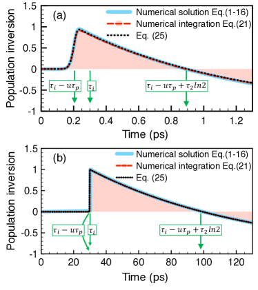
Figure 2: (Color online) Population inversion $I(t,z=0)$ for (a) $(\tau_{2},\tau_{i})=(1\mathrm{ps},0.3\mathrm{ps})$ and (b) $(\tau_{2},\tau_{i})=(100\mathrm{ps},30\mathrm{ps})$. Thick-blue-solid, red-dashed-filled and black-dotted lines depict $\rho_{22}(t,0)-\rho_{11}(t,0)$ from the numerical solution of Eq. (1-16), numerical integration of Eq. (III) and Eq. (25), respectively. Three downward green arrows chronologically indicate three key temporal instants, namely, $\tau_{i}-u\tau_{p}$, $\tau_{i}$ and $\tau_{i}-u\tau_{p}+\tau_{2}\ln 2$. The gain duration of $I(t,z)>0$ is about $\tau_{2}\ln 2$. Other parameters are $(r,n_{p},\tau_{p},\sigma)=(2\mu\mathrm{m},30\times 10^{12},60\mathrm{fs},3.336\times 10^{-23}\mathrm{m^{2}})$.

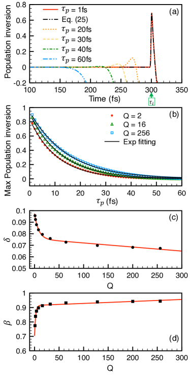
Figure 3: (Color online) (a) population inversion $I(t,z=0)$ for $(\tau_{2},\tau_{i})=(10\mathrm{fs},300\mathrm{fs})$ and a range of $J_{p}$ pulse duration based on XFEL parameter, namely, $\tau_{p}=1$fs (red solid line), $\tau_{p}=20$fs (orange dotted line), $\tau_{p}=30$fs (yellow dashed line), $\tau_{p}=40$fs (green dashed-dotted line) and $\tau_{p}=60$fs (blue dashed-dashed-dotted-dotted line). Black dashed-dotted-dotted line is Eq. (25). Other parameters are $(n_{p},\tau_{p},r,\sigma)=(QT_{p}\times 10^{12},T_{p}\mathrm{fs},2\mu\mathrm{m},3.336\times 10^{-23}\mathrm{m^{2}})$ and $Q=1$. Upward green arrow indicates $\tau_{i}$. (b) the max population inversion as a function of $T_{p}$ for $Q=2$ (red dots), $Q=16$ (green triangles) and $Q=256$ (blue squares). Black solid lines are $\beta e^{-\delta T_{p}}$ fittings. (c) $Q$-dependent $\delta$. (d) $Q$-dependent $\beta$.

III Analytical solutions

Given the XFEL pulse duration $\leq$100 fs and possible wide range of $\tau_{2}$ for different systems, it is necessary to analyse the influence of temporal structure of pumping pulse on the production of population inversion. In this section we analyse the pumping process in the region of $|\Omega^{\pm}|\ll\Gamma<J_{p}\sigma$, namely, pumping rate is greater than excited state decay rate and photon emission rate, which allows for the production of population inversion. By first using $\rho_{00}\left(t,z\right)=1$, the solution of Eq. (6) reads

$$J_{p}(t,z)=\frac{n_{p}}{\pi^{3/2}r^{2}\tau_{p}}\mathrm{Exp}\left[-n\sigma z-\left(\frac{t-\tau_{i}-\frac{z}{c}}{\tau_{p}}\right)^{2}\right].$$ (19)

In the parameter region of Fig. 2 and Fig. 3, $\mathrm{Exp}\left(-n\sigma L\right)>0.98$, one can therefore neglect the attenuation of $J_{p}$ for both cases. The solution of Eq. (1) is then given by

$$\rho_{00}(t,z)\approx\mathrm{Exp}\left\{-\frac{n_{p}\sigma}{2\pi r^{2}}\left[1+\mathrm{erf}\left(\frac{t-\tau_{i}-\frac{z}{c}}{\tau_{p}}\right)\right]\right\}.$$ (20)

The dynamics of $\rho_{22}$ obey $\partial_{t}\rho_{22}=\sigma J_{p}\rho_{00}-\Gamma\rho_{22}$ whose solution reads

$$\rho_{22}(t)\approx\frac{n_{p}\sigma}{\pi^{3/2}r^{2}\tau_{p}}\mathrm{Exp}\left(-\Gamma t-\frac{n_{p}\sigma}{2\pi r^{2}}\right)$$

$$\times \int_{0}^{t}\mathrm{Exp}\left[\Gamma s-\frac{n_{p}\sigma}{2\pi r^{2}}\mathrm{erf}\left(\frac{s-\tau_{i}}{\tau_{p}}\right)-\left(\frac{s-\tau_{i}}{\tau_{p}}\right)^{2}\right]ds.$$

Invoking the conservation of population $\sum_{i=1}^{3}\rho_{ii}(t,z)=1$ one gets $\rho_{11}$. A careful comparison confirms that Eq. (III) is equivalent to the numerical solution of complete Eqs. (1-16). When $\tau_{p}<\tau_{2}$, we can obtain approximate solutions

$$\rho_{22}(t,z) \approx \left[1-\rho_{00}(t)\right]e^{-\Gamma\left(t-\tau_{i}-\frac{z}{c}+u\tau_{p}\right)},$$ (22)

$$\rho_{11}(t,z) \approx \left[1-\rho_{00}(t)\right]\left[1-e^{-\Gamma\left(t-\tau_{i}-\frac{z}{c}+u\tau_{p}\right)}\right],$$ (23)

$$u = 2+\frac{e\pi^{3/2}r^{2}}{n_{p}\sigma}\left(1-\sqrt{1+\frac{4n_{p}\sigma}{e\pi^{3/2}r^{2}}}\right),$$ (24)

where $u\tau_{p}$ corresponds to $\partial^{2}_{t}\rho_{00}(t)|_{t=u\tau_{p}}=0$ when the maximum consumption rate of $\rho_{00}$ by $J_{p}$ occurs, and $e$ is Euler’s number. One can also obtain the approximate population inversion $I(t,z)=\rho_{22}(t,z)-\rho_{11}(t,z)$

$$I(t,z)\approx\left[1-\rho_{00}(t,z)\right]\left[2e^{-\Gamma\left(t-\tau_{i}-\frac{z}{c}+u\tau_{p}\right)}-1\right].$$ (25)

Figure 2 demonstrates the comparison between the numerical solution of complete Eqs. (1-16), the numerical integration of Eq. (III) and the analytical solution of Eq. (25) for $\tau_{2}=1$ps and $\tau_{2}=100$ps. This plainly demonstrates the consistency between the three methods. When the time scale of $\tau_{2}$ is small and approaching $\tau_{p}$, the effect caused by the leading edge of the $J_{p}$ pulse becomes significant, i.e., the shift $u\tau_{p}$ of around 0.2ps in Fig. 2(a). The peak value of $I(t,z)$ actually happens at about $\tau_{i}+\frac{z}{c}-u\tau_{p}$ instead of $\tau_{i}+\frac{z}{c}$. The temporal shift of $u\tau_{p}$, namely, the spacing between the first two downward green arrows, reveals that the subsequent emissions may overtake $J_{p}$. The excited atoms subsequently experience spontaneous decay, and give a similar duration of $\tau_{2}\ln 2$, i.e., the spacing between first and third downward green arrows, for positive $I(t,z)$. This gain domain, e.g., $[0.2\mathrm{ps},0.9\mathrm{ps}]$ in Fig. 2(a) and $[30\mathrm{ps},98\mathrm{ps}]$ in Fig. 2(b), is the energy reservoir for ASE while outside the region $\Omega^{\pm}$ will be reabsorbed by atoms in the ground state. On can accordingly define the transient gain length $L_{g}=c\tau_{p}/2$ in the medium. The analysis of $I(t,z)$ is important for the understanding of the ASE gain curve, which will be performed in what follows.

In order to investigate the gain process of $\Omega^{+}$, we further approximate

$$I(t,z)\approx\left[2e^{-\Gamma\left(t-\tau_{i}-\frac{z}{c}+u\tau_{p}\right)}-1\right]\Theta\left(t-\tau_{i}-\frac{z}{c}+u\tau_{p}\right),$$ (26)

where $\Theta$ is the Heaviside unit step function, and solve the simplified equations $\partial_{t}\rho_{21}^{+}=-\frac{i}{2}PI\Omega^{+}$ and $\partial_{z}\Omega^{+}=i\eta\rho_{21}^{+}$. The integral of the former leads to $\rho_{21}^{+}(t,z)=-\frac{i}{2}P\int_{0}^{t}\Omega^{+}(\tau,z)I(\tau,z)d\tau$ which is then substituted into the latter. We arrive at

$$\partial_{z}\Omega^{+}(t,z) = \frac{P\Gamma\alpha}{4L}\int_{0}^{t}\Omega^{+}(\tau,z)I(\tau,z)d\tau$$ (27)

$$\approx \Omega^{+}(t,z)\frac{P\Gamma\alpha}{4L}\int_{0}^{t}I(\tau,z)d\tau.$$

Neglecting $\partial_{t}\Omega^{+}$ in the wave equation is justified when Eq. (26) goes to the retarded time frame, namely, as a function of $t-\frac{z}{c}$ Bonifacio et al. (1975); MacGillivray and Feld (1976); Rai and Bowden (1992). The additional factor $P$ indicates the weighting of the forward emission. In the early stage, i.e., $\Gamma\gg|\Omega^{+}|$, spontaneous emission dominates, and so $P=1/2$ is expected in the simplified equations because an atom has the equal chance for the forward/backward spontaneous emission. We further neglect the temporal structure of $\Omega^{+}(t,z)$ and extract it from the integrand of Eq. (27). The peak value of output $\Omega^{+}$ pulse in the end of the medium $(z=L)$ reads

$$\Omega^{+}(L) \approx \Omega^{+}_{0}\mathrm{Exp}\left\{\frac{P\Gamma\alpha}{4L}\int_{0}^{L}\int_{\tau_{l}}^{\tau_{u}}I(\tau,z)d\tau dz\right\}$$ (28)

$$= \Omega^{+}_{0}e^{\xi\alpha}.$$

Here $\Omega^{+}_{0}$ is given by Gaussian white noise, and $\tau_{l}=\tau_{i}+\frac{z}{v}$, $\tau_{u}=\tau_{i}+\frac{z}{c}-u\tau_{p}+\tau_{2}\ln 2$. Because $\Omega^{+}$ is always behind $J_{p}$ and must stay in the gain interval $\left[\tau_{l},\tau_{u}\right]$, where the population inversion $I>0$, as demonstrated in Fig. 2. The gain factor $2\xi$ is then determined to be

$$2\xi=\frac{P}{4}\left\{\frac{L\Gamma}{v}-\frac{L\Gamma}{c}+2u\tau_{p}\Gamma-2-\ln 4-\frac{4cv}{\left(c-v\right)L\Gamma}e^{-u\tau_{p}\Gamma}\left[e^{\left(\frac{1}{c}-\frac{1}{v}\right)L\Gamma}-1\right]\right\}.$$ (29)

The upper bound of $2\xi$ in Eq. (29) occurs when $v$ approaches $c$, namely,

$$\lim_{v\to c}2\xi=\frac{P}{2}\left(2e^{-u\tau_{p}\Gamma}+u\tau_{p}\Gamma-1-\ln 2\right),$$ (30)

which results in the maximum gain exponent. One can deduce the range of the group velocity $v$ of the emitted light pulse as follows. Given the fact that the $\Omega^{+}$ pulse propagates with group velocity $v$ all the way behind $J_{p}$ and so $v<c$. Since the emitted light must stay in the gain domain illustrated in Fig. 2 when $I\left(t,z\right)>0$, otherwise it will be re-absorbed, we have the gain condition $\tau_{i}+\frac{z}{c}\leq\tau_{l}\leq\tau_{u}$. This indicates that $J_{p}$ produces population inversion at $z$ during $\left[\tau_{i}+\frac{z}{c},\tau_{u}\right]$ where we neglect the small correction of $u\tau_{p}$ in the lower bound, but $\Omega^{+}$ passes through $z$ at $\tau_{l}$ which must be within the above gain interval. The inverse of the gain condition leads to the range of $v$

$$c\geq v\geq\frac{cL\Gamma}{L\Gamma+c\ln 2-c\Gamma u\tau_{p}}.$$ (31)

We analyse the trajectory of the emitted pulse and observe that the group velocity $v$ is initially smaller than $c$ and gradually approaches $c$ when the optical ringing effect occurs. While the acceleration mechanism remains an interesting theoretical topic to be studied, one can still use Eq. (30) to estimate the upper bound of ASE gain exponent.

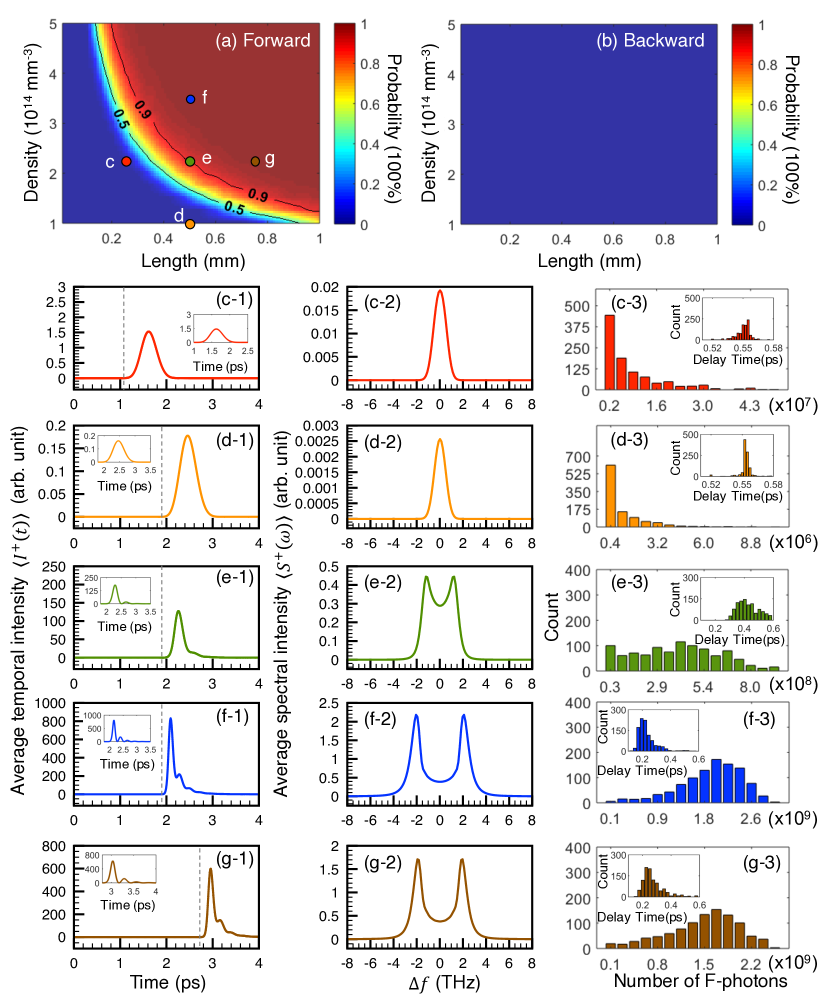
Figure 4: (Color online) Probability of (a) forward $\int_{-\infty}^{\infty}|\Omega^{+}\left(t,L\right)|dt\geq\frac{\pi}{2}$ and that of (b) backward $\int_{-\infty}^{\infty}|\Omega^{-}\left(t,0\right)|dt\geq\frac{\pi}{2}$ as a function of ($L$, $n$) among 1000 realizations with Gaussian random noise for ($r$, $n_{p}$, $\tau_{p}$, $\tau_{2}$)=(2$\mu$m, 30$\times 10^{12}$, 60fs, 1ps). Five data sets, marked as c ($L$, $n$) = (0.25mm, 2.25$\times 10^{14}$mm^-3), d (0.5mm, 1$\times 10^{14}$mm^-3), e (0.5mm, 2.25$\times 10^{14}$mm^-3), f (0.5mm, 3.5$\times 10^{14}$mm^-3) and g (0.75mm, 2.25$\times 10^{14}$mm^-3) in (a), are picked up to show the transition from amplified spontaneous emission to superfluorescence of $\Omega^{+}$. The corresponding average temporal intensity, average spectral intensity and photon number histogram of each chosen point are respectively illustrated by ($\textbf{x}-1$), ($\textbf{x}-2$) and ($\textbf{x}-3$), where $\textbf{x}\in\left\{\textbf{c},\textbf{b},\textbf{e},\textbf{f},\textbf{g}\right\}$. Gray dashed lines in (c-1)-(g-1) indicate instants when $J_{p}$ leaves the medium. Insets in (c-1)-(g-1) and (c-3)-(g-3) demonstrate the typical $|\Omega^{+}\left(t,L\right)|^{2}$ of a single realization and delay time histogram of forward emission at each chosen set of parameters, respectively.

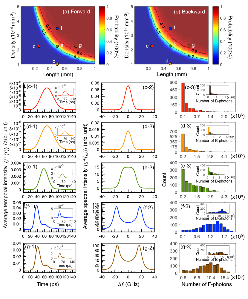
Figure 5: (Color online) Probability of (a) forward $\int_{-\infty}^{\infty}|\Omega^{+}\left(t,L\right)|dt\geq\frac{\pi}{2}$ and that of (b) backward $\int_{-\infty}^{\infty}|\Omega^{-}\left(t,0\right)|dt\geq\frac{\pi}{2}$ as a function of ($L$, $n$) among 1000 realizations with Gaussian random noise for ($r$, $n_{p}$, $\tau_{p}$, $\tau_{2}$)=(2$\mu$m, 30$\times 10^{12}$, 60fs, 100ps). Five data sets, marked as c ($L$, $n$) = (0.25mm, 2.25$\times 10^{14}$mm^-3), d (0.5mm, 1$\times 10^{14}$mm^-3), e (0.5mm, 2.25$\times 10^{14}$mm^-3), f (0.5mm, 3.5$\times 10^{14}$mm^-3) and g (0.75mm, 2.25$\times 10^{14}$mm^-3) in (a) and (b), are chosen for showing the transition from amplified spontaneous emission to superfluorescence. The corresponding average temporal intensity, average spectral intensity and photon number histogram of the forward emission at each chosen point are respectively illustrated by ($\textbf{x}-1$), ($\textbf{x}-2$) and ($\textbf{x}-3$), where $\textbf{x}\in\left\{\textbf{c},\textbf{b},\textbf{e},\textbf{f},\textbf{g}\right\}$. The corresponding average temporal intensity and photon number histogram of the backward emission are illustrated in the insets of (c-1)-(g-1) and those of (c-3)-(g-3), respectively.

In view of the time structure of XFEL Eur and the recent XFEL-pumped laser Rohringer et al. (2012), we investigate the pumping process with a variety of XFEL parameters Eur . Fig. 3(a) illustrates the numerical solution of $I(t,0)$ for $\tau_{2}=10$fs with a variety of $\tau_{p}$. We use $(n_{p},\tau_{p},\tau_{i},r)=(QT_{p}\times 10^{12},T_{p}\mathrm{fs},300\mathrm{fs},2\mu\mathrm{m})$ and $Q=1$ to fix the amplitude of $J_{p}$ at a constant $4.5\times 10^{37}$ s^-1m^-2 when varying $T_{p}$. The red solid line depicts the case for $\tau_{p}=1$fs, i.e., $T_{p}=1$ in which $J_{p}$ is short enough to generate population inversion between state $|2\rangle$ and $|1\rangle$ with a peak value of 0.69. As one can see, the analytical solution Eq. (25) (black dashed-dotted-dotted line) also matches the numerical integration of Eq. (III) (red solid line) as $\tau_{p}<\tau_{2}$. When $\tau_{p}\geq\tau_{2}$, the analysis of Eq. (III) becomes a complicated problem, and the competition between the $\sigma J_{p}$ and $\Gamma$ terms in Eq. (3) causes $I(t,z)$ to exhibit more complicated behaviour. For long pumping pulses of $\tau_{p}=20$fs (orange dotted line), $\tau_{p}=30$fs (yellow dashed line), $\tau_{p}=40$fs (green dashed-dotted line) and $\tau_{p}=60$fs (blue dashed-dashed-dotted-dotted line), the $\tau_{p}$-dependent reduction of population inversion is observed. Such a reduction is caused by the consumption of $\rho_{00}$ by the leading edge of $J_{p}$ whose pumping power is too weak to compete against the fast decay of state $|2\rangle$. The leading edge of $J_{p}$ and the decay rate $\Gamma$ turn the medium transparent before the arrival of the peak of $J_{p}$. Fig. 3(b-c) show that the increase of the amplitude of $J_{p}$ slightly eases the reduction of population inversion due to the leading edge of $J_{p}$. In Fig. 3(b) we use $Q=2$ (red dots), $Q=16$ (green triangles) and $Q=256$ (blue squares) to demonstrate the effect of increasing the $J_{p}$ amplitude on the maximum population inversion as a function of $T_{p}$. The black solid lines are $\beta e^{-\delta T_{p}}$ fittings. The $Q$-dependent $\delta$ and $\beta$ are respectively depicted in Fig. 3(c) and Fig. 3(d). As one can see in Fig. 3(c) that, in the $Q$ domain of $\left[1,300\right]$, $\delta$ ranges between 0.07 to 0.1 corresponding to a variety of $\tau_{p}$ between 10fs and 15fs. When $\tau_{p}$ is shorter than this range, transient population inversion can be built up and this results in a noticeable gain of $\Omega^{\pm}$. For $\tau_{p}>40$fs population inversion is suppressed and the gain of $\Omega^{\pm}$ becomes negligible. Consequently, the temporal structure of a pumping pulse plays a more critical role than $J_{p}$ amplitude does when $\tau_{p}$ and $\tau_{2}$ are in a similar time scale. When $\tau_{p}$ is too long, the pumping capability of a $J_{p}$ pulse will degrade. The rapid decrease of $\delta$ in Fig. 3(c) and the quick increase of $\beta$ in Fig. 3(d) for $Q<$ 20 suggest that there is an efficient choice of $J_{p}$ amplitude to optimize the generation of population inversion. It is worth mentioning that the red solid fitting curves in Fig. 3(c & d) are in the form of $a+be^{-fQ}+gQ$, where $a$, $b$, $f$ and $g$ are some fitting constants, which may provide useful information for future analytical study of $I(t,z)$.

IV Numerical Results

Here we turn to the discussion of the numerical solution of Eq. (1-16). Fig. 4 demonstrates the results of ($r$, $n_{p}$, $\tau_{p}$, $\tau_{2}$) = (2$\mu$m, 30$\times 10^{12}$, 60fs, 1ps) and Fig. 5 shows that of ($r$, $n_{p}$, $\tau_{p}$, $\tau_{2}$) = (2$\mu$m, 30$\times 10^{12}$, 60fs, 100ps). Fig. 4 (a) and Fig. 5 (a) depict the probability of forward emission $\int_{-\infty}^{\infty}|\Omega^{+}\left(t,L\right)|dt\geq\frac{\pi}{2}$ among 1000 realizations of simulation at each point of ($L$, $n$). Fig. 4 (b) and Fig. 5 (b) depict that of backward emission $\int_{-\infty}^{\infty}|\Omega^{-}\left(t,0\right)|dt\geq\frac{\pi}{2}$. In the forward emission for both $\tau_{2}=1$ps and $\tau_{2}=100$ps, the growth of the area of $\Omega^{+}$ and its gain are observed when either the length of the medium $L$ or the density of the medium $n$ increases. However, for backward emission, the similar tendency only occurs when $\tau_{2}=100$ps but is absent for $\tau_{2}=1$ps. Fig. 4 (b) reveals that no matter how one changes the parameters of a gain medium the backward pulse area $\int_{-\infty}^{\infty}|\Omega^{-}\left(t,0\right)|dt$ is always negligible. This forward-backward asymmetry will be discussed in Sec. V.

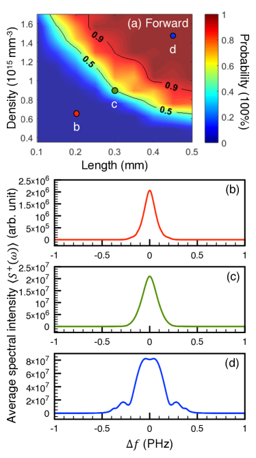
Figure 6: (Color online) (a) Probability of $\int_{-\infty}^{\infty}|\Omega^{+}\left(t,L\right)|dt\geq\frac{\pi}{2}$ occurs as a function of ($L$, $n$) in forward direction among 1000 realizations with Gaussian random noise for ($r$, $n_{p}$, $\tau_{p}$, $\tau_{2}$)=(2$\mu$m, $10^{14}$, 24fs, 10fs). $\alpha\simeq 1760$ for probability of 50%. The average spectral intensity of five data sets, marked as b ($L$, $n$) = (0.2mm, 6.5$\times 10^{14}$mm^-3), c (0.3mm, 9.5$\times 10^{14}$mm^-3), d (0.44mm, 1.48$\times 10^{15}$mm^-3), are chosen for showing the transition from amplified spontaneous emission to superfluorescence of $\Omega^{+}$.

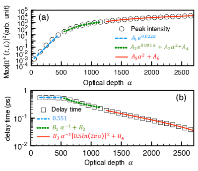
Figure 7: (Color online) $\alpha$-dependent (a) peak intensity and (b) delay time of the emitted pulse $|\Omega^{+}(t,L)|^{2}$ for $\tau_{2}=1$ps. Black circles and black squares respectively represent peak intensity and delay time from numerical solutions of $|\Omega^{+}(t,L)|^{2}$. Each color line illustrates a fitting curve in the correspond $\alpha$ domain. All parameters are those used in Fig.4. The fitting coefficients are $\left(A_{1},A_{2},A_{3},A_{4},A_{5},A_{6}\right)=$ ( $4.72\times 10^{-4}$, $-5.42\times 10^{3}$, $8.65\times 10^{-3}$, $6.82\times 10^{3}$, $1.96\times 10^{-3}$, $-1.66\times 10^{3}$) and $\left(B_{1},B_{2},B_{3},B_{4}\right)=$ ( $2.97\times 10^{2}$, $-1.86\times 10^{-2}$, $2.11\times 10$, $-1.5\times 10^{-1}$).

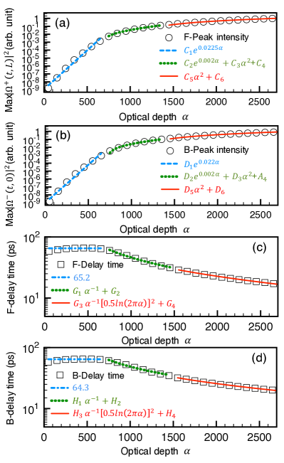
Figure 8: (Color online) $\alpha$-dependent peak intensity of (a) forward $|\Omega^{+}(t,L)|^{2}$ and (b) backward $|\Omega^{-}(t,0)|^{2}$ for $\tau_{2}=100$ps. $\alpha$-dependent delay time of the emitted pulse (c) $|\Omega^{+}(t,L)|^{2}$ and (d) $|\Omega^{-}(t,0)|^{2}$. Black circles and black squares respectively represent peak intensity and delay time from numerical solutions. Each color line illustrates a fitting curve in the correspond $\alpha$ domain. All parameters are those used in Fig.5. The fitting coefficients are $\left(C_{1},C_{2},C_{3},C_{4},C_{5},C_{6}\right)=$ ( $1.21\times 10^{-9}$, $0.021$, $-7.38\times 10^{-8}$, $-0.05$, $1.7\times 10^{-7}$, $-0.22$), $\left(D_{1},D_{2},D_{3},D_{4},D_{5},D_{6}\right)=$ ( $1.05\times 10^{-9}$, $0.016$, $-5.46\times 10^{-8}$, $-0.04$, $1.41\times 10^{-7}$, $-0.18$), $\left(G_{1},G_{2},G_{3},G_{4}\right)=$ ( $4.58\times 10^{4}$, $3.96\times 10^{-1}$, $2.5\times 10^{3}$, $-5.258$) and $\left(H_{1},H_{2},H_{3},H_{4}\right)=$ ( $4.2\times 10^{4}$, $6.77$, $2.53\times 10^{3}$, $-2.47$).

In both Fig. 4(a) and Fig. 5(a) there are five data sets marked as c ($L$, $n$) = (0.25mm, 2.25$\times 10^{14}$mm^-3), d (0.5mm, 1$\times 10^{14}$mm^-3), e (0.5mm, 2.25$\times 10^{14}$mm^-3), f (0.5mm, 3.5$\times 10^{14}$mm^-3) and g (0.75mm, 2.25$\times 10^{14}$mm^-3). Average temporal intensity based on Eq. (17), average spectral intensity calculated by Eq. (18) and photon number histogram of five chosen points are respectively demonstrated by ($\textbf{x}-1$), ($\textbf{x}-2$) and ($\textbf{x}-3$) of Fig. 4 and Fig. 5, where $\textbf{x}\in\left\{\textbf{c},\textbf{b},\textbf{e},\textbf{f},\textbf{g}\right\}$. When scanning parameters through either path c-e-g of lengthening the gain medium with constant density or d-e-f of densifing the gain medium for a given length, we observe that the pulse area becomes high, and the occurrence of optical ringing and spectral splitting becomes significant. The typical $|\Omega^{+}\left(t,L\right)|^{2}$ of single realization are illustrated by the insets of Fig. 4($\textbf{x}-1$). One can see that the optical ringing effect happens in $\int_{-\infty}^{\infty}|\Omega^{+}\left(t,L\right)|dt\geq\frac{\pi}{2}$ region. The shortening of the $\Omega^{+}(t,L)$ pulse duration is accompanied by the widening of spectral splitting. The delay time between the peak of $J_{p}(t,L)$ and the peak of $\Omega^{+}(t,L)$ also becomes short, namely speed-up emission. For a better visualization, we indicate the peak instant of $J_{p}(t,L)$ by gray dashed lines in Fig. 4($\textbf{x}-1$), and it is very close to $t=0$ in Fig. 5($\textbf{x}-1$) of longer time scale. We demonstrate the time delay histogram of forward emission for $\tau_{2}=1$ps in the insets of Fig. 4($\textbf{x}-3$). One can see that the most probable delay time is shifting to small value, and its fluctuation amplitude becomes ten times wide when the probability of $\int_{-\infty}^{\infty}|\Omega^{+}\left(t,L\right)|dt\geq\frac{\pi}{2}$ increases. Moreover, Fig. 4($\textbf{x}-3$) and Fig. 5($\textbf{x}-3$) show that the photon number histogram of the emitted $\Omega^{+}(t,L)$ spreads from left to the right and gradually peaks at a certain large photon number. As also revealed by Fig. 4($\textbf{x}-3$) and Fig. 5($\textbf{x}-3$), the fluctuation amplitude of photon number is also getting wide when the system goes to high optical depth region. The $\langle I^{-}\left(t\right)\rangle$ and backward photon number histogram are illustrated in Fig. 5($\textbf{x}-1$) inset and Fig. 5($\textbf{x}-3$) inset, respectively. Both share the same tendency with the forward one. The above features suggest that $\Omega^{\pm}$ experiences a certain transition Okada et al. (1978); Brechignac and Cahuzac (1981); Malcuit et al. (1987) around the boundary of $\int_{-\infty}^{\infty}|\Omega^{+}\left(t,L\right)|dt=\frac{\pi}{2}$ and $\int_{-\infty}^{\infty}|\Omega^{-}\left(t,0\right)|dt=\frac{\pi}{2}$ which is associated with Rabi oscillation. For $\tau_{2}=10$fs, our numerical simulation shows that the population inversion is not produced by $J_{p}$ when $\tau_{p}>30$fs. This confirms the analysis demonstrated in Fig. 3(a) using the integral approach. Fig. 6 illustrates the results utilizing ($r$, $n_{p}$, $\tau_{p}$, $\tau_{2}$)=(2$\mu$m, $10^{14}$, 24fs, 10fs). Because the backward emission is negligible in this case, we only depict the probability of forward emission in Fig. 6(a). The three data sets are marked as b ($L$, $n$) = (0.2mm, 6.5$\times 10^{14}$mm^-3), c (0.3mm, 9.5$\times 10^{14}$mm^-3) and d (0.44mm, 1.48$\times 10^{15}$mm^-3), and their corresponding spectra of $\Omega^{+}(t,L)$ are given in Fig. 6(b), (c) and (d), respectively. When moving to the top right along path b-c-d, the spectrum is getting split. This reflects the slightly oscillatory behaviour damped by the high decay rate in the time domain, and the similar transition also happens around $\int_{-\infty}^{\infty}|\Omega^{+}\left(t,L\right)|dt=\frac{\pi}{2}$ and $\int_{-\infty}^{\infty}|\Omega^{-}\left(t,0\right)|dt=\frac{\pi}{2}$.

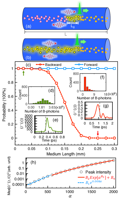
Figure 9: (Color online) Forward and backward asymmetry and length induced backward transition. All particles are initially prepared in state $|0\rangle$ (orange-filled circles). (a) as $L_{g}<L$, pumped particles remain in excited state $|2\rangle$ (yellow dots) for only a short distance behind the pumping pulse (green-right-moving Gaussian), and others decay to state $|1\rangle$ (red shaded circles). (b) case when $L_{g}>L$. (c) probability of forward $\int_{-\infty}^{\infty}|\Omega^{+}\left(t,L\right)|dt\geq\frac{\pi}{2}$ (blue solid line) and that of backward $\int_{-\infty}^{\infty}|\Omega^{-}\left(t,0\right)|dt\geq\frac{\pi}{2}$ (red dashed line) as a function of $L$ among 1000 realizations for $\left(\tau_{2},\alpha\right)=$ (1ps, 1500). Other parameters are the same as those used in Fig. 4. (d) backward photon number histogram and (e) $\langle I^{-}\left(t\right)\rangle$ for $L=0.025$mm (indicated by green upward arrow). (f) backward photon number histogram and (g) $\langle I^{-}\left(t\right)\rangle$ for $L=0.25$mm (indicated by red downward arrow). Gray dashed lines indicate instants when $J_{p}$ leaves the medium. (h) $\alpha-$dependent average backward peak intensity for $L=0.25$mm. Fitting parameters $\left(B_{1},B_{2},B_{3},B_{4}\right)=$ ( $5.57\times 10^{-5}$, $6.07\times 10^{-8}$, $3.78\times 10^{-1}$, $4.52\times 10^{-4}$)

In order to quantify the observed transition, we collect $|\Omega^{+}(t,L)|^{2}$ and $|\Omega^{-}(t,0)|^{2}$ for each contour in Fig. 4&5 and analyse them by finding the $\alpha$ power law for the averaged peak intensity and for the averaged delay time between forward/backward emission and the output pumping pulse. In Fig. 7(a) and Fig. 8(a)(b) the black circles depict the $\alpha$-dependent peak intensity. In Fig. 7(b) and Fig. 8(c)(d) the black squares demonstrate the $\alpha$-dependent delay time. The blue dashed lines are fitting curves for $\alpha\leq 500$, green dotted line for $500<\alpha<1200$ and red solid lines for $\alpha>1200$. In Fig.7 and Fig.8 the domain $500<\alpha<1200$ and $700<\alpha<1500$ are obviously the watershed of power law, respectively. To the left of the watershed the peak intensity exhibits exponential growth with a constant delay time of 0.551 ps for $\tau_{2}=1$ps and that of about 65ps for $\tau_{2}=100$ps, which typically results from ASE. The upper bound of the ASE gain exponent of 0.055 and that of 0.076 are given by Eq. (30) for $\tau_{2}=1$ps and $\tau_{2}=100$ps, respectively. Both are in the same order of magnitude with the fitting value of 0.022 (blue dashed line in Fig. 7(a) and Fig. 8(a)(b)). However, to the right of the watershed the peak intensity is proportional to $\alpha^{2}$, and the delay time behaves as the typical form of $\tau_{D}\propto\alpha^{-1}\left[\frac{1}{2}\ln\left(2\pi\alpha\right)\right]^{2}$ Rehler and Eberly (1971); Polder et al. (1979); Gross and Haroche (1982). The former corresponds to the collective emission and the latter reflects the needed time for building up coherence from noise Polder et al. (1979); Gross and Haroche (1982), which are both signatures of superfluorescence. It is worth mentioning that the typical form of superfluorescence delay time deviates from the numerical values when $\alpha<1200$ and $\alpha<1500$ for $\tau_{2}=1$ps and $\tau_{2}=100$ps, respectively. In the watershed domain, the green dotted line in Fig. 7(a) and Fig. 8(a)(b) indicate that the peak intensity behaves as a superposition of exponential growth and $\alpha^{2}$. This tendency reveals that a transition does happen from one emission mechanism to another Okada et al. (1978); Malcuit et al. (1987). The present results also suggest that the optical depth $\alpha$ plays the key role for a transition from ASE to SF. This transition happens at the boundary where Rabi oscillation also starts to occur. The validity of one dimensional simulation is associated with the Fresnel number condition $\mathbf{F}=\frac{\pi r^{2}}{L\lambda}\approx 1$. Otherwise one has to deal with full three-dimensional wave propagation in simulations for the transverse effect of diffraction Gross and Haroche (1982), which consumes a lot of computational time and power especially for the ensemble average. To avoid such heavy computation, we have compared averaged results due to different values of $n$ and $L$ for $nL=$ constant, i.e., $\alpha=$ constant, in our model and do not observe any significant difference. Therefore, one could take the advantage of the $\alpha$-dependent features and effectively use a system which fulfils the Fresnel condition with the same $\alpha$.

Given that the boundary between ASE and SF may occur when $\int_{-\infty}^{\infty}\Omega\left(t\right)dt=\frac{\pi}{2}$, we here estimate the photon number of an emitted $\frac{\pi}{2}$-pulse. For simplicity, we use a Gaussian pulse such that $\int_{-\infty}^{\infty}\Omega Exp\left[-\left(\frac{t}{\kappa\tau_{2}}\right)^{2}\right]dt\approx\Omega\sqrt{\pi}\kappa\tau_{2}=\frac{\pi}{2}$ where $\kappa\tau_{2}$ is the duration of the emitted pulse, and $\kappa=\ln 2$ given by the duration of positive population inversion as illustrated in Fig. 2. One can therefore obtain $\Omega\approx\frac{\sqrt{\pi}}{2\tau_{2}\ln 2}$. In view of the fact that the integral of laser intensity equals the energy of $n_{e}$ photons, $\frac{1}{2}c\varepsilon_{0}\pi r^{2}\int_{-\infty}^{\infty}\frac{\hbar^{2}}{d^{2}}|\Omega\left(t\right)|^{2}dt=n_{e}\hbar\omega$, which results in $n_{e}\approx\frac{\hbar c\varepsilon_{0}\pi^{5/2}r^{2}}{8\sqrt{2}\omega d^{2}\ln 2}\Gamma$. By substituting $c=\omega\lambda/\left(2\pi\right)$ and the spontaneous decay rate $\Gamma=\frac{d^{2}\omega^{3}}{3\pi\varepsilon_{0}\hbar c^{3}},$ we obtain

$$n_{e}\approx\frac{\pi^{\frac{7}{2}}r^{2}}{6\sqrt{2}\lambda^{2}\ln 2},$$ (32)

which suggests that $n_{e}$ of a $\frac{\pi}{2}$-pulse mainly depends on the ratio of $r$ to $\lambda$. In the present cases, $n_{e}=1.75\times 10^{7}$ is very close to our numerical result of $3.24\times 10^{7}$.

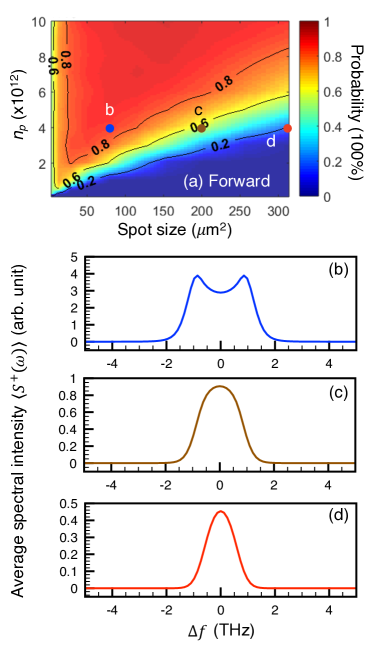
Figure 10: (Color online) (a) probability of superfluorescence occurs as a function of ($\pi r^{2}$, $n_{p}$) in forward direction among 1000 realizations for $\left(L,n,\tau_{2}\right)=\left(0.16\mathrm{mm},5\times 10^{14}\mathrm{mm^{-3}},1\mathrm{ps}\right)$ with Gaussian random noise. Three data sets, marked as b (78.54$\mu$m², 4$\times 10^{12}$), c (201.06$\mu$m², 4$\times 10^{12}$), d (314.16$\mu$m², 4$\times 10^{12}$) in (a), are chosen for showing the transition from amplified spontaneous emission to superfluorescence. The corresponding average spectra are respectively illustrated in (b), (c) and (d).

V Length-Induced Backward Transition

We turn to investigate the forward-backward asymmetry demonstrated in Fig. 4(a)(b) and its relation with $L_{g}$ and $L$. Fig. 9(a) shows that regions sandwich the small gain area (filled with yellow shaded circles) causes an asymmetric environment for light propagating forwards and backwards. For $L_{g}<L$ there is always a gain medium ($\rho_{22}>\rho_{11}$) ahead for light propagating forward, but an absorption medium ($\rho_{22}<\rho_{11}$) for the backward radiation. This is one of reasons why backward emission is often absent in a swept pumping system. In contrast, Fig. 9(b) reveals that choosing a system with $L_{g}>L$ will lead to symmetric behaviour for both directions. As a result, the increase of $\Omega^{-}$ gain and events of $\int_{-\infty}^{\infty}|\Omega^{-}\left(t,0\right)|dt\geq\frac{\pi}{2}$ are observed for $\tau_{2}=100$ps in Fig. 5 (b).

Given $L_{g}=0.15$mm for $\tau_{2}=1$ps as demonstrated in Fig. 2(a), the backward superfluorescence is anticipated to show up as $L<0.15$mm but not when $L>0.15$mm. In what follows we use constant $\alpha=1500$ and same parameters used in Fig. 4 to demonstrate length induced backward ASE-SF transition in Fig. 9(c). The blue solid line and red dashed line respectively represent the probability of $\int_{-\infty}^{\infty}|\Omega^{+}\left(t,L\right)|dt\geq\frac{\pi}{2}$ and that of $\int_{-\infty}^{\infty}|\Omega^{-}\left(t,0\right)|dt\geq\frac{\pi}{2}$ among 1000 realizations of simulation for each length. Fig. 9(d) and (e) show backward photon number histogram and $\langle I^{-}\left(t\right)\rangle$, respectively for $L=0.025$mm, and Fig. 9(f)(g) for $L=0.25$mm. $J_{p}$ leaves the medium at the instants pointed out by gray dashed lines. As one would expect from Fig. 4(a) that forward probability remains 100% for the whole length range. However, the backward emission reveals five interesting features when shortening $L$ across the critical value of $L_{g}=0.15$mm: (1) probability noticeably raises to 100%; (2) $\langle I^{-}\left(t\right)\rangle$ catches up $J_{p}$; (3) backward light pulse exits the medium earlier than $J_{p}$ does when $L\gtrsim L_{g}$ as depicted by Fig. 9(g); (4) photon number histogram demonstrates similar ASE-SF transition as depicted in Fig. 4 and 5; (5) $\langle I^{-}\left(t\right)\rangle$ manifests optical ringing as illustrated by Fig.9(g) (also in single cases). Above features support our picture of the length effect and are consistent with Fig. 2(a) and Eq. (25) which is the consequence of $J_{p}\left(t,0\right)$ and $\tau_{2}$. The tiny pulse peaks at $t=1.3$ps in Fig.9(g) suggests that the backward emission from region deeper than $L_{g}$ is possible. In view that the backward pulse area for $L\gtrsim L_{g}$ in Fig. 9(c) is mostly smaller than $\pi/2$, one would expect it is in the low gain and linear region. However, the optical ringing is never observed in the ASE region of Fig.5, and so feature (5) raises the following question for backward emission. Why can small pulse area and optical ringing coexist in the range of $L_{g}\sim L$ but cannot in $L_{g}>L$? Since the backward pulse duration in Fig. 9(g) is shorter than $\tau_{2}$ limited by $L_{g}$, a broadband small-area pulse envelope should also oscillate when propagating through a resonant medium of high optical depth Crisp (1970). This will not happen to forward ASE because the gain medium co-moves along with it, making forward ASE duration always comparable to $\tau_{2}$, i.e., narrowband, as demonstrated in Fig. 4 and 5. Nevertheless, the non-oscillating ASE in Fig. 5 suggests there is other mechanism than Ref.Crisp (1970), namely, attenuating SF. Because $\alpha=1500$ is very high, the backward emission can quickly grow into SF in the gain region and then enters the dissipative but still penetrable area such that small pulse area and optical ringing can coexist in the range of $L_{g}\sim L$. In Fig. 9(h) we depict average backward peak intensity as function of $\alpha$ by varying $n$ but fixing $L=0.25$mm. Each point is also an average over 1000 realizations of simulation. The fitting shows that $\Omega^{-}\left(t,0\right)$ do experience a transition at around $\alpha=500$ and manifests nonlinear evolution lower than $\alpha^{2}$ dependence. In contrast, the forward light behaves identically as that in Fig. 7. Similar study for $L=0.025$mm also shows identical ASE-SF transition for both forward and backward emissions. Our backward study suggests that (I) a triggered small-area ASE by an external seeding pulse shorter than $\tau_{2}$ may lead to also an oscillating ASE in both forward and backward direction due to the mechanism of Ref.Crisp (1970); and (II) the transverse pumping may ease the forward-backward asymmetry.

VI Transition induced by XFEL $J_{p}$ Laser parameters

It is a natural question to ask whether one could manipulate $\Omega^{+}$ by changing $J_{p}$ laser Skribanowitz et al. (1973); MacGillivray and Feld (1976); Cui et al. (2013); Cui and Macovei (2017) based on XFEL parameter Eur . In Fig. 10(a) we demonstrate the probability of the occurrence of $\int_{-\infty}^{\infty}|\Omega^{+}\left(t,L\right)|dt\geq\frac{\pi}{2}$ as a function of $(\pi r^{2},n_{p})$. In our simulation, the pumping photon flux is affected by both $r$ and $n_{p}$ as denoted by Eq. (13), and the Gaussian white noise also depends on $r$ as indicated by Eq. (16). Given the short lifetime $\tau_{2}=1$ps, gain growth only happens to the forward emissions. We use $\left(L,n,\tau_{2}\right)=\left(0.16\mathrm{mm},5\times 10^{14}\mathrm{mm^{-3}},1\mathrm{ps}\right)$ to numerically solve Eq.(1-16) for 1000 realizations of simulation at each combination of $J_{p}$ laser spot size and photon number. The three data sets are marked as b (78.54$\mu$m², 4$\times 10^{12}$), c (201.06$\mu$m², 4$\times 10^{12}$) and d (314.16$\mu$m², 4$\times 10^{12}$) in Fig. 10(a). Their averaged spectra based in Eq. (18) is respectively demonstrated in Fig. 10(b), (c) and (d). When scanning parameters through the b-c-d path of shrinking $J_{p}$ spot size and fixing pumping photon number, the occurrence of spectral splitting also becomes obvious. As a consequence, one can manipulate the properties of emitted $\Omega^{\pm}$ not only by changing the parameters of the gain medium but also by altering that of pumping laser $J_{p}$.

VII Summary

We have demonstrated the transition between ASE and SF in a three-level-$\Lambda$ type system induced by the change of optical depth of a medium and by the alternation of pumping XFEL parameters, namely, focus spot size and pulse energy. A consistent picture of the transition from one region to another suggested by the Maxwell-Bloch equation is summarized in what follows. A pencil-shape gain medium is longitudinally and incoherently pumped by a short XFEL pulse, and then the inverted medium experiences spontaneous decay. Although the spontaneously emitted photons go to all directions, a small number of forward emitted photons follow the XFEL pulse and enter the solid angle $\varphi$, as demonstrated in Fig. 1, within which photons may subsequently interact with other excited particles. The backward emitted photons may also interact with the inverted particles or may be reabsorbed by the pre-decayed particles behind the gain region depending on $L_{g}\geq L$ or $L_{g}<L$, respectively (see Fig. 9). Due to the geometry, the forward emitted light and the backward one, in the above former case, are both amplified along the long axis of the gain medium. As the pulse area approaches $\pi/2$, the ASE-SF transition starts to occur and results in, e.g., optical ringing effect, spectral splitting and the change in statistics behaviours as demonstrated in Fig. 4,  5, 7 and 8. We have investigated the pumping procedure in detail using XFEL parameters and identified $L_{g}$ and $L$ as two key parameters making forward-backward asymmetry. Moreover, in the region of $L_{g}\gtrsim L$,we have also studied the length-induced backward transition for the first time. The present results demonstrate a controllable single-pass light source whose properties can be manipulated by parameters of a medium or those of a pumping XFEL.

VIII Acknowledgement

We thank Jason Payne for carefully reading our manuscript. Y.-H. K. and W.-T. L. are supported by the Ministry of Science and Technology, Taiwan (Grant No. MOST 107-2112-M-008-007-MY3 and Grant No. MOST 107-2745-M-007-001-). W.-T. L. is also supported by the National Center for Theoretical Sciences, Taiwan.

References

- Dicke (1954) R. H. Dicke, Phys. Rev. 93, 99 (1954).
- Polder et al. (1979) D. Polder, M. F. H. Schuurmans, and Q. H. F. Vrehen, Phys. Rev. A 19, 1192 (1979).
- Gross and Haroche (1982) M. Gross and S. Haroche, Physics reports 93, 301 (1982).
- Skribanowitz et al. (1973) N. Skribanowitz, I. P. Herman, J. C. MacGillivray, and M. S. Feld, Phys. Rev. Lett. 30, 309 (1973).
- Gross et al. (1976) M. Gross, C. Fabre, P. Pillet, and S. Haroche, Phys. Rev. Lett. 36, 1035 (1976).
- Gibbs et al. (1977) H. M. Gibbs, Q. H. F. Vrehen, and H. M. J. Hikspoors, Phys. Rev. Lett. 39, 547 (1977).
- Paradis et al. (2008) E. Paradis, B. Barrett, A. Kumarakrishnan, R. Zhang, and G. Raithel, Phys. Rev. A 77, 043419 (2008).
- Florian et al. (1984) R. Florian, L. O. Schwan, and D. Schmid, Phys. Rev. A 29, 2709 (1984).
- Malcuit et al. (1987) M. S. Malcuit, J. J. Maki, D. J. Simkin, and R. W. Boyd, Phys. Rev. Lett. 59, 1189 (1987).
- Dreher et al. (2004) M. Dreher, E. Takahashi, J. Meyer-ter Vehn, and K.-J. Witte, Phys. Rev. Lett. 93, 095001 (2004).
- Noe II et al. (2012) G. T. Noe II, J.-H. Kim, J. Lee, Y. Wang, A. K. Wójcik, S. A. McGill, D. H. Reitze, A. A. Belyanin, and J. Kono, Nature Physics 8, 219 (2012).
- Deacon et al. (1977) D. A. G. Deacon, L. R. Elias, J. M. J. Madey, G. J. Ramian, H. A. Schwettman, and T. I. Smith, Phys. Rev. Lett. 38, 892 (1977).
- Nagasono et al. (2011) M. Nagasono, J. R. Harries, H. Iwayama, T. Togashi, K. Tono, M. Yabashi, Y. Senba, H. Ohashi, T. Ishikawa, and E. Shigemasa, Phys. Rev. Lett. 107, 193603 (2011).
- Mercadier et al. (2019) L. Mercadier, A. Benediktovitch, C. Weninger, M. A. Blessenohl, S. Bernitt, H. Bekker, S. Dobrodey, A. Sanchez-Gonzalez, B. Erk, C. Bomme, et al., Phys. Rev. Lett. 123, 023201 (2019).
- Watanabe et al. (2007) T. Watanabe, X. J. Wang, J. B. Murphy, J. Rose, Y. Shen, T. Tsang, L. Giannessi, P. Musumeci, and S. Reiche, Phys. Rev. Lett. 98, 034802 (2007).
- Cui et al. (2012) N. Cui, M. Macovei, K. Z. Hatsagortsyan, and C. H. Keitel, Phys. Rev. Lett. 108, 243401 (2012).
- Cui et al. (2013) N. Cui, C. H. Keitel, and M. Macovei, Opt. Lett. 38, 570 (2013).
- Cui and Macovei (2017) N. Cui and M. A. Macovei, Phys. Rev. A 96, 063814 (2017).
- Keitel et al. (1992) C. H. Keitel, M. O. Scully, and G. Süssmann, Phys. Rev. A 45, 3242 (1992).
- Kozlov et al. (1999) V. Kozlov, O. Kocharovskaya, Y. Rostovtsev, and M. Scully, Phys. Rev. A 60, 1598 (1999).
- Pert (1994) G. Pert, J. Opt. Soc. Am. B 11, 1425 (1994).
- Rohringer et al. (2012) N. Rohringer, D. Ryan, R. A. London, M. Purvis, F. Albert, J. Dunn, J. D. Bozek, C. Bostedt, A. Graf, R. Hill, et al., Nature 481, 488 (2012).
- Weninger and Rohringer (2014) C. Weninger and N. Rohringer, Phys. Rev. A 90, 063828 (2014).
- Yoneda et al. (2015) H. Yoneda, Y. Inubushi, K. Nagamine, Y. Michine, H. Ohashi, H. Yumoto, K. Yamauchi, H. Mimura, H. Kitamura, T. Katayama, et al., Nature 524, 446 (2015).
- Schuurmans and Polder (1979) M. Schuurmans and D. Polder, Physics Letters A 72, 306 (1979).
- Shvyd’ko et al. (1996) Y. V. Shvyd’ko, T. Hertrich, U. van Bürck, E. Gerdau, O. Leupold, J. Metge, H. D. Rüter, S. Schwendy, G. V. Smirnov, W. Potzel, et al., Phys. Rev. Lett. 77, 3232 (1996).
- Röhlsberger et al. (2010) R. Röhlsberger, K. Schlage, B. Sahoo, S. Couet, and R. Rüffer, Science 328, 1248 (2010).
- Liao et al. (2011) W.-T. Liao, A. Pálffy, and C. H. Keitel, Physics Letters B 705, 134 (2011).
- Röhlsberger et al. (2012) R. Röhlsberger, H. C. Wille, K. Schlage, and B. Sahoo, Nature 482, 199 (2012).
- Liao et al. (2012) W.-T. Liao, A. Pálffy, and C. H. Keitel, Phys. Rev. Lett. 109, 197403 (2012).
- Adams et al. (2013) B. W. Adams, C. Buth, S. M. Cavaletto, J. Evers, Z. Harman, C. H. Keitel, A. Pálffy, A. Picón, R. Röhlsberger, Y. Rostovtsev, et al., Journal of modern optics 60, 2 (2013).
- Liao et al. (2013) W.-T. Liao, A. Pálffy, and C. H. Keitel, Phys. Rev. C 87, 054609 (2013).
- Vagizov et al. (2014) F. Vagizov, V. Antonov, Y. Radeonychev, R. Shakhmuratov, and O. Kocharovskaya, Nature 508, 80 (2014).
- Liao and Pálffy (2014) W.-T. Liao and A. Pálffy, Phys. Rev. Lett. 112, 057401 (2014).
- Heeg et al. (2015) K. P. Heeg, J. Haber, D. Schumacher, L. Bocklage, H.-C. Wille, K. S. Schulze, R. Loetzsch, I. Uschmann, G. G. Paulus, R. Rüffer, et al., Phys. Rev. Lett. 114, 203601 (2015).
- Liao and Ahrens (2015) W.-T. Liao and S. Ahrens, Nature Photon. 9, 169 (2015).
- Heeg et al. (2017) K. P. Heeg, A. Kaldun, C. Strohm, P. Reiser, C. Ott, R. Subramanian, D. Lentrodt, J. Haber, H.-C. Wille, S. Goerttler, et al., Science 357, 375 (2017).
- Wang and Liao (2018) G.-Y. Wang and W.-T. Liao, Phys. Rev. Applied 10, 014003 (2018).
- Bonifacio et al. (1971a) R. Bonifacio, P. Schwendimann, and F. Haake, Phys. Rev. A 4, 302 (1971a).
- Bonifacio et al. (1971b) R. Bonifacio, P. Schwendimann, and F. Haake, Phys. Rev. A 4, 854 (1971b).
- Okada et al. (1978) J. Okada, K. Ikeda, and M. Matsuoka, Opt. Commun. 27, 321 (1978).
- Brechignac and Cahuzac (1981) C. Brechignac and P. Cahuzac, J. Phys. B 14, 221 (1981).
- Rai and Bowden (1992) J. Rai and C. M. Bowden, Phys. Rev. A 46, 1522 (1992).
- Haake et al. (1979a) F. Haake, H. King, G. Schröder, J. Haus, R. Glauber, and F. Hopf, Phys. Rev. Lett. 42, 1740 (1979a).
- Haake et al. (1979b) F. Haake, H. King, G. Schröder, J. Haus, and R. Glauber, Phys. Rev. A 20, 2047 (1979b).
- Arecchi and Courtens (1970) F. T. Arecchi and E. Courtens, Phys. Rev. A 2, 1730 (1970).
- Bonifacio et al. (1975) R. Bonifacio, F. A. Hopf, P. Meystre, and M. O. Scully, Phys. Rev. A 12, 2568 (1975).
- Hopf and Meystre (1975) F. A. Hopf and P. Meystre, Phys. Rev. A 12, 2534 (1975).
- (49) Beam parameters of european xfel radiation, URL http://xfel.desy.de/technical_information/photon_beam_parameter/.
- Friedberg and Hartmann (1976) R. Friedberg and S. R. Hartmann, Phys. Rev. A 13, 495 (1976).
- Gunst et al. (2014) J. Gunst, Y. A. Litvinov, C. H. Keitel, and A. Pálffy, Phys. Rev. Lett. 112, 082501 (2014).
- ten Brinke et al. (2013) N. ten Brinke, R. Schützhold, and D. Habs, Phys. Rev. A 87, 053814 (2013).
- Zhang and Svidzinsky (2013) X. Zhang and A. A. Svidzinsky, Phys. Rev. A 88, 033854 (2013).
- MacGillivray and Feld (1976) J. C. MacGillivray and M. S. Feld, Phys. Rev. A 14, 1169 (1976).
- Yuan and Svidzinsky (2012) L. Yuan and A. A. Svidzinsky, Phys. Rev. A 85, 033836 (2012).
- Lin et al. (2009) Y.-W. Lin, W.-T. Liao, T. Peters, H.-C. Chou, J.-S. Wang, H.-W. Cho, P.-C. Kuan, and A. Y. Ite, Phys. Rev. Lett. 102, 213601 (2009).
- Liao and Pálffy (2014) W.-T. Liao and A. Pálffy, Phys. Rev. Lett. 112, 057401 (2014).
- Su et al. (2016) S.-W. Su, Z.-K. Lu, S.-C. Gou, and W.-T. Liao, Scientific reports 6, 35402 (2016).
- Vrehen and der Weduwe (1981) Q. H. F. Vrehen and J. J. der Weduwe, Phys. Rev. A 24, 2857 (1981).
- Rehler and Eberly (1971) N. E. Rehler and J. H. Eberly, Phys. Rev. A 3, 1735 (1971).
- Crisp (1970) M. D. Crisp, Phys. Rev. A 1, 1604 (1970).