Precessional spin-torque dynamics in biaxial antiferromagnets

Abstract

The Néel order of an antiferromagnet subject to a spin torque can undergo precession in a circular orbit about any chosen axis. To orient and stabilize the motion against the effects of magnetic anisotropy, the spin polarization should have components in-plane and normal to the plane of the orbit, where the latter must exceed a threshold. For biaxial antiferromagnets, the precessional motion is described by the equation for a damped-driven pendulum, which has hysteresis a function of the spin current with a critical value where the period diverges. The fundamental frequency of the motion varies inversely with the damping, and as $(x^{p}-1)^{1/p}$ with the drive-to-criticality ratio $x$ and the parameter $p>2$. An approximate closed-form result for the threshold spin current is presented, which depends on the minimum cutoff frequency the orbit can support. Precession about the hard axis has zero cutoff frequency and the lowest threshold, while the easy axis has the highest cutoff. A device setup is proposed for electrical control and detection of the dynamics, which is promising to demonstrate a tunable terahertz nano-oscillator.

I Introduction

In antiferromagnetic materials, injection of a spin current exerts spin torque on alternating spin moments, which can excite steady-state precession of the Néel order at terahertz frequencies Gomonay and Loktev (2014). The precession can reciprocally pump spins into an adjacent conductor Vaidya et al. (2020), which may generate an oscillating sinusoidal Khymyn et al. (2017) or spike-like Khymyn et al. (2018) electric signal. These electrically-induced antiferromagnetic oscillations could serve as compact narrowband terahertz sources and spike generators for applications in terahertz imaging and sensing Mittleman (2017), and in neuromorphic computing Torrejon et al. (2017).

Given a source of spin current, how does the spin torque affect the dynamics of the Néel-order? In biaxial-anisotropy antiferromagnets, this problem has been studied for special cases where the spin current is polarized either along the easy or hard anisotropy axis . The description of the motion for a general angle of spin polarization and parametric study of the nonlinear dynamics are, however, unexplored, which we we analyze in this paper in detail. This topic has implications for a tunable terahertz detector Gomonay et al. (2018), which can filter frequencies higher than a certain cutoff frequency determined by the precession axis.

We study the precession of Néel order caused by spin torque about an arbitrary rotational axis. The equation of motion (Sec. II) permits steady-state solutions where the Néel order precesseses in a circular orbit (Sec. III). The dynamics is analyzed separately into angular motion in the orbit which determines the frequency (Sec. III.1), and perturbation from the orbital plane which determines the stability (Sec: III.2). A schema for electrical control and detection of antiferromagnetic dynamics is presented in Sec. IV.

II Theoretical framework

Antiferromagnets with a bipartite collinear ordering Dombre and Read (1989) are composed of two interpenetrating square lattices $A$ and $B$ with oppositely aligned moments. For such ordering, the thermodynamic state of the antiferromagnet in a mean-field approximation is represented by the unit vectors $\mathbf{m}_{A}$ and $\mathbf{m}_{B}$ for the sublattice spin moments, each of which has a magnetization $M_{\text{s}}$ Kittel (2004). There are three significant contributions to the free energy density of an antiferromagnet: the exchange coupling of neighboring spins, the magnetocrystalline anisotropy, and the Zeeman interaction of magnetic moments with an external magnetic field.

Biaxial-anisotropy antiferromagnets are characterized by a direction of minimum energy which is ‘easy’ for spins to orient along, and an orthogonal direction of maximum energy which is ‘hard’. Consider a monodomain film of thickness $d_{\text{a}}$ with the easy and hard axes oriented along the unit vectors $\mathbf{u}_{\text{e}}$ and $\mathbf{u}_{\text{h}}$, respectively (Fig. 1). If the antiferromagnetic exchange coupling between the sublattice moments is much stronger than the anisotropy, the average net moment $\mathbf{m}=(\mathbf{m}_{A}+\mathbf{m}_{B})/2$ and the Néel order $\mathbf{n}=(\mathbf{m}_{A}-\mathbf{m}_{B})/2$ satisfy the relation $\mathbf{n}^{2}=1-\mathbf{m}^{2}\approx 1$. The total free energy density in the presence of an external magnetic field $H$ applied along the unit vector $\mathbf{h}$ up to lowest order is Qaiumzadeh et al. (2017); Parthasarathy and Rakheja (2019a)

$$\mathcal{F}=\mathcal{J}\mathbf{m}^{2}+\mathcal{K}_{\text{h}}(\mathbf{n}\cdot\mathbf{u}_{\text{h}})^{2}-\mathcal{K}_{\text{e}}(\mathbf{n}\cdot\mathbf{u}_{\text{e}})^{2}-2\mathcal{Z}\mathbf{m}\cdot\mathbf{h},$$ (1)

where the exchange coupling $\mathcal{J}$, the anisotropy coefficients $\mathcal{K}_{i}$ and the Zeeman energy density $\mathcal{Z}=\mu_{0}M_{\text{s}}H$ are positive numbers, and $\mathcal{J}\gg\mathcal{K}_{i},\mathcal{Z}$.

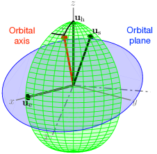
Figure 1: Representation of magnetic-anisotropy easy axis $\mathbf{u}_{\text{e}}$ and hard axis $\mathbf{u}_{\text{h}}$, spin-polarization direction $\mathbf{u}_{\text{s}}$, and steady-state circular orbit of Néel order on a unit-sphere quadrant.

In the limit of large exchange, the problem of coupled dynamics of the sublattice moments approximately reduces to motion of the Néel order on a unit-sphere phase space Kosevich et al. (1990); Gomonay and Loktev (2010). Starting from the Landau-Lifshitz-Gilbert equation augmented with the antidamping-like torque Slonczewski (1996); Sinova et al. (2015); Jungwirth et al. (2016) induced by a spin current, the $\sigma$-model equation of motion for the Néel order is Kosevich et al. (1990); Parthasarathy and Rakheja (2019a)

$$\mathbf{n}\times\bigg{[}\frac{M_{\text{s}}}{\gamma\mathcal{J}}\ddot{\mathbf{n}}+\alpha\dot{\mathbf{n}}+\frac{\gamma}{M_{\text{s}}}(\mathcal{K}_{\text{h}}(\mathbf{n}\cdot\mathbf{u}_{\text{h}})\mathbf{u}_{\text{h}}-\mathcal{K}_{\text{e}}(\mathbf{n}\cdot\mathbf{u}_{\text{e}})\mathbf{u}_{\text{e}})+$$

$$\frac{\mathcal{Z}}{\mathcal{J}}\big{(}2\dot{\mathbf{n}}\times\mathbf{h}+\gamma\mu_{0}H(\mathbf{n}\cdot\mathbf{h})\mathbf{h}\big{)}+\frac{\gamma J_{\text{s}}}{M_{\text{s}}d_{\text{a}}}(\mathbf{n}\times\mathbf{u}_{\text{s}})\bigg{]}=0,$$ (2)

where an overdot denotes derivative with respect to time $t$, $\alpha>0$ is the Gilbert damping, $\gamma$ is the absolute gyromagnetic ratio, and $J_{\text{s}}$ is the injected spin-current density with non-equilibrium spin polarization along the unit vector $\mathbf{u}_{\text{s}}$ . The equation is second order, implying that Néel-order has inertia. The net moment Parthasarathy and Rakheja (2019a)

$$\mathbf{m}=\frac{M_{\text{s}}}{\gamma\mathcal{J}}(\dot{\mathbf{n}}\times\mathbf{n})+\frac{\mathcal{\mathcal{\mathcal{Z}}}}{\mathcal{J}}[\mathbf{h}-(\mathbf{n}\cdot\mathbf{h})\mathbf{n}]$$ (3)

becomes a dependent variable, allowing for the Néel order dynamics (2) to be solved independently.

Multiplying Eq. (2) by $M_{\text{s}}/(\gamma\mathcal{K}_{\text{e}})$, when the external field is much smaller than spin-flop field $\mathcal{\mathcal{Z}}\ll\sqrt{\mathcal{J}\mathcal{K}_{\text{e}}}$ , the $\mathcal{Z}$-coefficient terms need not be considered. In dimensionless form, where the time is scaled by characteristic frequency $\tau_{0}=t(\gamma\sqrt{\mathcal{J}\mathcal{K}_{\text{e}}}/M_{\text{s}})$, the equation of motion becomes

$$\mathbf{n}\times[\mathbf{n}^{\prime\prime}+\beta_{0}\mathbf{n}^{\prime}+\kappa(\mathbf{n}\cdot\mathbf{u}_{\text{h}})\mathbf{u}_{\text{h}} -(\mathbf{n}\cdot\mathbf{u}_{\text{e}})\mathbf{u}_{\text{e}}$$

$$+\Gamma_{0}(\mathbf{n}\times\mathbf{u}_{\text{s}})/2]=0,$$ (4)

where a prime denotes derivative with respect to $\tau_{0}$, and the dimensionless parameters are defined as $\beta_{0}=\alpha\sqrt{\mathcal{J}/\mathcal{K}_{\text{e}}}$, $\kappa=\mathcal{K}_{\text{h}}/\mathcal{K}_{\text{e}}$ and $\Gamma_{0}=2J_{\text{s}}/(\mathcal{K}_{\text{e}}d_{\text{a}})$. From hereafter, $\Gamma_{0}\mathbf{u}_{\text{s}}$ is called the spin-polarization vector.

III Analysis of solution

In steady state, Eq. (4) can have stationary solutions $\mathbf{n}^{\prime}=0$ and time-varying solutions $\mathbf{n}^{\prime}\neq 0$ depending on the parameters and initial condition,. Vector product of Eq. (4) with the angular speed $\mathbf{n}\times\mathbf{n}^{\prime}$ followed by dot product with $\mathbf{n}$ produces

$$\kappa(\mathbf{n}\cdot\mathbf{u}_{\text{h}})[( \mathbf{n}\times\mathbf{n}^{\prime})\cdot\mathbf{u}_{\text{h}}]-(\mathbf{n}\cdot\mathbf{u}_{\text{e}})[(\mathbf{n}\times\mathbf{n}^{\prime})\cdot\mathbf{u}_{\text{e}}]$$

$$+(\mathbf{n}\times\mathbf{n}^{\prime})\cdot\mathbf{n}^{\prime\prime}+\Gamma_{0}(\mathbf{n}^{\prime}\cdot\mathbf{u}_{\text{s}})/2=0,$$ (5)

the relationship between the projection of $\mathbf{u}_{\text{e}}$, $\mathbf{u}_{\text{h}}$ and $\mathbf{u}_{\text{s}}$ on the orthogonal vectors $\mathbf{n}$, $\mathbf{n}^{\prime}$ and $\mathbf{n}\times\mathbf{n}^{\prime}$.

Among time-varying solutions, we claim that $(\mathbf{n}\times\mathbf{n}^{\prime})\cdot\mathbf{n}^{\prime\prime}=0$ is a subset wherein the Néel order precesses in a circular orbit around the origin. Let the orbital axis make a polar angle $\Theta$ from the hard axis along $z$ and an azimuthal angle $\Phi$ from the easy axis along $x$ as shown in Fig. 1, with intermediate axis along $y$. The orthonormal basis suitable for the orbital plane is defined as $\mathbf{\tilde{x}}=[\cos\Theta\cos\Phi,\cos\Theta\sin\Phi,-\sin\Theta]$, $\mathbf{\tilde{y}}=[-\sin\Phi,\cos\Phi,0]$ and $\mathbf{\tilde{z}}=[\sin\Theta\cos\Phi,\sin\Theta\sin\Phi,\cos\Theta]$. If the Néel order makes an angle $\phi$ counterclockwise from $\mathbf{\tilde{x}}$ axis in the orbital plane and rotates with angular speed $\phi^{\prime}$, $\mathbf{n}=\mathbf{\tilde{x}}\cos\phi+\mathbf{\tilde{y}}\sin\phi$ and $\mathbf{n}^{\prime}=\phi^{\prime}(-\mathbf{\tilde{x}}\sin\phi+\mathbf{\tilde{y}}\cos\phi)$. On substitution into Eq. (5), the orbital axis orients along $(\Theta,\Phi)$ if the components of the spin-polarization vector in the orbital plane satisfy

$$\Gamma_{0}(\mathbf{\tilde{x}}\cdot\mathbf{u}_{\text{s}}) =\sin(\Theta)\sin(2\Phi),$$ (6a)

$$\Gamma_{0}(\mathbf{\tilde{y}}\cdot\mathbf{u}_{\text{s}}) =(\kappa+\cos^{2}\Phi)\sin(2\Theta),$$ (6b)

and $\phi^{\prime}\neq 0$, which requires the perpendicular component $\Gamma_{0}(\mathbf{\tilde{z}}\cdot\mathbf{u}_{\text{s}})$ to overcome a certain threshold to drive the motion against damping. Determining this condition requires analyzing the angular motion and stability of the orbiting Néel order.

III.1 Angular motion in orbit

Equation (4) implies that tangential components of $\mathbf{n}$ inside the square bracket should vanish. Equating the component $\bm{\phi}=-\mathbf{\tilde{x}}\sin\phi+\mathbf{\tilde{y}}\cos\phi$ to zero gives the angular motion in the orbital plane

$$2\phi^{\prime\prime} +2\beta_{0}\phi^{\prime}+[\cos(2\Phi)-(\kappa+\cos^{2}\Phi)\sin^{2}\Theta]\sin(2\phi)$$

$$+[\cos\Theta\sin(2\Phi)]\cos(2\phi)=\Gamma_{0}(\mathbf{\tilde{z}}\cdot\mathbf{u}_{\text{s}}).$$ (7)

Combining $\sin(2\phi)$ and $\cos(2\phi)$ terms together, and performing the following replacements

$$C=\cos(2\Phi)-(\kappa+\cos^{2}\Phi)\sin^{2}\Theta,\quad D=\cos\Theta\sin(2\Phi);$$

$$g=\sqrt{C^{2}+D^{2}},\quad\beta=\frac{\beta_{0}}{\sqrt{g}},\quad\tau=\frac{\tau_{0}}{\sqrt{g}}\quad\Gamma=\frac{\Gamma_{0}\absolutevalue{\mathbf{\tilde{z}}\cdot\mathbf{u}_{\text{s}}}}{g};$$

$$\varphi=\mathrm{sgn}(\mathbf{\tilde{z}}\cdot\mathbf{u}_{\text{s}})\left[2\phi+\arctan(\frac{D}{C})\right];$$ (8)

recast the equation of motion into (derivative denoted by prime for $\varphi$ are with respect to $\tau$)

$$\varphi^{\prime\prime}+{\beta}\varphi^{\prime}+\sin\varphi={\Gamma},$$ (9)

that of a unit-mass pendulum of unit length in effective gravity $g$ with a viscous damping ${\beta}$ and driven by a constant tangential force ${\Gamma}$ Coullet et al. (2005).

The solution of the damped-driven pendulum equation (9) depends only on two dimensionless parameters $\beta$ and $\Gamma$. The steady-state dynamics of this non-linear system yields either a stationary solution [$\varphi^{\prime}(\tau)=0$], or a periodic solution [$\varphi^{\prime}(\tau+T)=\varphi^{\prime}(\tau)\neq 0$] with a period $T$. Transient simulation with initial conditions $\varphi_{0}=\pi$ and $\varphi^{\prime}_{0}=0$ over the parameter space is used to obtain the time $T$ to complete a revolution in steady state ($\tau>7/\beta$). A contour plot of the fundamental frequency is shown in Fig. 2 depicting the regions of different types of solutions.

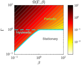
Figure 2: Fundamental frequency $\Omega$ (16) of the damped-driven pendulum equation (9) in the parameter space of effective damping $\beta$ and drive $\Gamma$ represented by contour map with values on colorbar.

In the hysteretic region, the steady-state solution can be periodic or stationary depending on the initial condition. For example, if the pendulum was released vertically upside down ($\varphi_{0}=\pi$), then it revolves continually; but if it was released horizontally from a point where the gravity opposes the drive ($\varphi_{0}=\pi/2$), then it dips and settles to equilibrium at $\sin\varphi_{\text{eq}}=\Gamma$. The hysteretic region is defined as: $f_{\text{h}}(\beta)<\Gamma(\beta)<1$ on the domain $0<\beta<\beta_{\text{h}}$, where $f_{\text{h}}$ determines the homoclinic bifurcation Strogatz (2018). The data is fit by a cubic-polynomial

$$f_{\text{h}}(\beta)=a_{0}\beta+\left(\frac{3-2a_{0}\beta_{\text{h}}}{\beta_{\text{h}}^{2}}\right)\beta^{2}+\left(\frac{a_{0}\beta_{\text{h}}-2}{\beta_{\text{h}}^{3}}\right)\beta^{3},$$ (10)

where $a_{0}=4/\pi$ Coullet et al. (2005) and $\beta_{\text{h}}\approx 1.2$. The minimum threshold drive needed to sustain revolutions (solid cyan line) is expressed

$$\Gamma_{\text{m}}(\beta)=\begin{cases}f_{\text{h}}(\beta)&\beta<\beta_{\text{h}}\\ 1&\beta\geq\beta_{\text{h}}\end{cases},$$ (11)

where $\Gamma_{\text{m}}=1$ is the threshold that can initiate revolutions independent of the damping (dashed cyan line).

In the overdrive limit $\Gamma\gg\Gamma_{\text{m}}$, the fundamental frequency is calculated by integrating Eq. (9) over a period and ignoring the role of gravity ($\sin\varphi$ term) to obtain

$$\Omega_{\text{O}\Gamma}=\frac{1}{2\pi}\frac{\Gamma}{\beta}.$$ (12)

This is consistent with the slope of the contour lines seen in Fig. 2 in regions far above the threshold. The time-dependence of the steady-state angular speed $\omega=\varphi^{\prime}$ is estimated from Eq. (9) by truncating $\sin\varphi\simeq\sin(\Gamma\tau\beta)$, multiplying by $e^{\beta\tau}$, integrating and letting the transients decay to give

$$\omega_{\text{O}\Gamma}(\tau)\simeq\frac{\Gamma}{\beta}-\frac{\beta}{\sqrt{\beta^{4}+\Gamma^{2}}}\sin(\frac{\Gamma}{\beta}\tau-\xi_{\text{O}\Gamma}),$$ (13)

where $\xi_{\text{O}\Gamma}=\arctan(\Gamma/\beta^{2})$.

In the overdamped limit $\beta\gg 1$, Eq. (9) reduces to $\varphi^{\prime}=(\Gamma-\sin\varphi)/\beta$, which is separable and has a closed-form integral. The periodic solution is expressed Coullet et al. (2005)

$$\Gamma\tan\frac{\varphi_{\text{O}\beta}(\tau)}{2}=1+\sqrt{\Gamma^{2}-1}\tan(\frac{\sqrt{\Gamma^{2}-1}}{2\beta}\tau-\xi_{\text{O}\beta}),$$

where $\xi_{\text{O}\beta}=\arctan(1/\sqrt{\Gamma^{2}-1})$. The fundamental frequency is

$$\Omega_{\text{O}\beta}=\frac{1}{2\pi}\frac{\sqrt{\Gamma^{2}-1}}{\beta},$$ (14)

and the steady-state angular speed is

$$\omega_{\text{O}\beta}(\tau)=\frac{\Gamma}{\beta}-\frac{2}{\beta}\frac{\tan(\varphi_{\text{O}\beta}/2)}{1+\tan^{2}(\varphi_{\text{O}\beta}/2)}.$$ (15)

Superposing the overdrive limit on Eq. (15) results in convergence of solutions with Eq. (13).

For moderate drive $\Gamma\gtrsim\Gamma_{\text{m}}$ and damping $\beta\lesssim 1$, it is not possible to derive analytic solutions Coullet et al. (2005); Gitterman (2008). However, the fundamental frequency closely follows the law

$$\Omega(\Gamma,\beta)=\frac{1}{2\pi}\frac{\big{[}\Gamma^{p}-\Gamma_{\text{m}}^{p}\big{]}^{1/p}}{\beta}\quad\quad\Bigg{\{}\begin{matrix}[l]\Gamma_{\text{m}}=\Gamma_{\text{m}}(\beta)\\[1.0pt] p=p(\beta)\end{matrix},$$ (16)

conceived by generalizing the overdamped result (14). The functional relationship $p(\beta)$ and the accuracy of the model are depicted in Fig. 3. The inverse dependence of $p$ on $\beta$ implies that a weakly damped system $\beta\ll 1$ is much easier to oscillate than a strongly damped $\beta\gg 1$ for a fixed drive-to-threshold ratio. Superposing the overdrive limit results in convergence with Eq. (12).

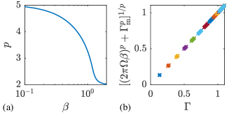
Figure 3: Plot of Eq. (16). (a) The parameter $p$ increases from 2 for $\beta\lesssim 1$. (b) The data for $\Omega$ evaluated with the vertical-axis function fits accurately with $\Gamma$, where adjoining markers of the same color have a unique $\beta$ (decreasing diagonally up).

To compare periodic solutions across the parameter space, the first-order term $\epsilon_{\text{O}\Gamma}=(\Gamma_{\text{m}}/\Gamma)^{p}/p$ in the expansion of $2\pi\beta\Omega/\Gamma$ (16) is used to measure nearness to overdrive; the relative increment $\epsilon_{\text{th}}=(\Gamma-\Gamma_{\text{m}})/\Gamma_{\text{m}}$ is used to measure nearness to threshold. The waveforms of the angular speed for limiting cases of damping and drive are juxtaposed in Fig. 4. The closed-form solutions agree with the numerical ones, except when the drive is near the minimum threshold and the damping is weak. The oscillations in angular speed are coherent in the overdrive limit, and Dirac-comb-like in the overdamped limit for near-threshold drive.

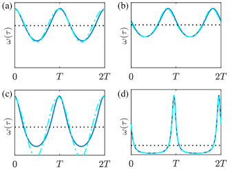
Figure 4: Waveforms of the steady-state angular speed $\omega(\tau)$ of the damped-driven pendulum revolving with time period $T$ for (a) overdrive $\epsilon_{\text{O}\Gamma}=0.05$ and small damping $\beta=0.2$, (b) overdrive $\epsilon_{\text{O}\Gamma}=0.05$ and large damping $\beta=5$, (c) near-threshold drive $\epsilon_{\text{th}}=0.05$ and small damping $\beta=0.2$, (d) near-threshold drive $\epsilon_{\text{th}}=0.05$ and large damping $\beta=5$. Dark-color plot is the exact numerical solution and light-color plot is the approximate closed-form solution. Dotted horizontal line denotes the average value equal to $2\pi\Omega$ (16). At time $\tau=0$, the pendulum is at the lowest point $\varphi=0$.

III.2 Stability of orbit

Orbits that are elevated from the plane perpendicular to hard axis may become stable only above a critical angular speed . To study stability, the Néel order is perturbed from the orbital plane by a small angle $\delta\theta$ or $\mathbf{n}=\mathbf{\tilde{x}}\cos\phi+\mathbf{\tilde{y}}\sin\phi+\mathbf{\tilde{z}}\delta\theta$. Equating the component $\bm{{\theta}}=(\mathbf{\tilde{x}}\cos\phi+\mathbf{\tilde{y}}\sin\phi)\delta\theta-\mathbf{\tilde{z}}$ inside the square bracket of Eq. (4) to zero, using the relation of Eq. (6), and retaining only linear terms in $\delta\theta$ gives the equation of a damped harmonic oscillator $\delta\theta^{\prime\prime}+\beta_{0}\delta\theta^{\prime}+K\delta\theta=0$, where the spring constant

$$K =\kappa(\cos^{2}\Theta-\sin^{2}\Theta\cos^{2}\phi)-\sin^{2}\Theta\cos^{2}\Phi$$

$$+(\cos\Theta\cos\Phi\cos\phi-\sin\Phi\sin\phi)^{2}+\phi^{\prime 2}.$$ (17)

To understand how $K$ depends on orbital parameters (8), expression (17) is expanded and compactly rewritten

$$K=\kappa-1-3\mathcal{E}+\frac{g}{2}\left(\cos\varphi+\frac{\varphi^{\prime 2}}{2}\right),$$ (18)

where the angle-averaged energy of the orbit

$$\mathcal{E} =\expectationvalue{\kappa(\mathbf{n}\cdot\mathbf{u}_{\text{h}})^{2}-(\mathbf{n}\cdot\mathbf{u}_{\text{e}})^{2}}$$

$$=\frac{1}{2}[(\kappa+\cos^{2}\Phi)\sin^{2}\Theta-1].$$ (19)

If $K$ is positive throughout the angular motion, the Néel order will restore to the orbital plane. The precise condition for stability for a general $\beta$ requires numerically evaluating the steady-state value of $(\cos\varphi+\varphi^{\prime 2}/2)$ in the parameter space of $\beta$ and $\Gamma$ (similar to how fundamental frequency was obtained in Sec. III.1), and checking if $\min_{\varphi}K>0$. But, an approximate closed-form result is obtained by treating $\varphi^{\prime}$ as a constant average value $2\pi\Omega$ (16), which is accurate in the overdrive limit. Then, the stability condition is $\min_{\varphi}K=g\pi^{2}\Omega^{2}-(g/2+3\mathcal{E}+1-\kappa)>0$, which gives the minimum angular frequency

$$\omega_{0}=\real(\sqrt{g/2+3\mathcal{E}+1-\kappa}\ \big{)},$$ (20)

which is positive for orientations satisfying $g/2+3\mathcal{E}+1-\kappa>0$ (Fig. 5). The stability threshold for perpendicular projection of the spin-polarization vector is

$$(\Gamma_{0}\absolutevalue{\mathbf{\tilde{z}}\cdot\mathbf{u}_{\text{s}}})_{\text{th}}=\left[\left(2\beta_{0}\omega_{0}\right)^{p}+\left\{g\Gamma_{\text{m}}(\beta_{0}/\sqrt{g})\right\}^{p}\right]^{1/p},$$ (21)

where $p=p(\beta_{0}/\sqrt{g})$ (Fig. 3a).

Figure 5: The minimum angular frequency $\omega_{0}$ (top) and threshold spin current $\Gamma_{0,\text{th}}$ (bottom) which can orient and stabilize the orbital motion of the Néel order about an axis $(\Theta,\Phi)$ when damping is small $\beta_{0}=0.2$ for uniaxial (left) and biaxial (right) anisotropy, represented by contour map with range of values on the colorbar (middle). The minimum frequency $\omega_{0}$ increases with deviation from the hard axis $(\Theta,\Phi)=(0,\Phi)$ and peaks along the easy axis $(\Theta,\Phi)=(\pi/2,0)$. The threshold is lowest for motion about the hard axis, and peaks for an intermediate orientation in-between hard and easy axis.

In essence, to orient and stabilize the orbital motion about an axis $(\Theta,\Phi)$, the spin-polarization vector

$$\Gamma_{0}\mathbf{u}_{\text{s}}=\sin(\Theta)\sin(2\Phi)\mathbf{\tilde{x}} +(\kappa+\cos^{2}\Phi)\sin(2\Theta)\mathbf{\tilde{y}}$$

$$+\Gamma_{0}(\mathbf{\tilde{z}}\cdot\mathbf{u}_{\text{s}})\mathbf{\tilde{z}},$$ (22)

where $\Gamma_{0}$ should exceed the threshold

$$\Gamma_{0,\text{th}}=\big{[}\sin^{2}(\Theta)\sin^{2}(2\Phi) +(\kappa+\cos^{2}\Phi)^{2}\sin^{2}(2\Theta)$$

$$+(\Gamma_{0}\absolutevalue{\mathbf{\tilde{z}}\cdot\mathbf{u}_{\text{s}})})_{\text{th}}^{2}\big{]}^{1/2}.$$ (23)

The spin-polarization direction does not coincide with the orbital axis, except for directions along the anisotropy axes for which $\Gamma_{0,\text{th}}=(\Gamma_{0}\absolutevalue{\mathbf{\tilde{z}}\cdot\mathbf{u}_{\text{s}}})_{\text{th}}$. The orbital parameters to orient along the anisotropy axes are as follows: hard axis has $(\Theta,\Phi)=(0,\Phi)$, $g=1$ and $\omega_{0}=0$, intermediate axis has $(\Theta,\Phi)=(\pi/2,\pi/2)$, $g=\kappa+1$ and $\omega_{0}=\sqrt{\kappa}$, and easy axis has $(\Theta,\Phi)=(\pi/2,0)$, $g=\kappa$ and $\omega_{0}=\sqrt{\kappa+1}$. The hard axis supports orbit with the lowest threshold and minimum angular frequency, while the easy axis has the highest cutoff. The axis along $(\Theta,\Phi)=(\arctan(1/\sqrt{\kappa}),0)$ has $g=0$ meaning no oscillations in angular speed. For small damping, the range of threshold varies from $4\beta_{0}/\pi$ to $\kappa+1$ (Fig. 5).

Below the threshold spin current, for moderate values of damping, the Néel-order motion can evolve into chaos (aperiodic long-term behavior) for a small window of current, before settling down to equilibrium, which will be the subject of future research.

Thus, the choice of the orbital axis, and the parameters of damping and anisotropy determine the threshold current, cutoff frequency and waveform of the angular speed of Néel order. These mathematical results may be translated into electrically measurable input and output signals via the device setup presented in the next section.

IV Electrical control and detection

Electrical means of controlling the spin current injected into the antiferromagnet and detecting the resulting oscillations in a thin-film system are fundamental to spintronic devices and applications in technology. In this regard, the setup should be all-electric with controllable spin-polarization direction.

Pure spin current through an insulating antiferromagnetic layer can be generated from electric current flowing in an overlaid lateral spin valve or spin Hall structure. In the lateral spin valve structure shown in Fig. 6a, electric current across the ferromagnetic reference layers injects spin accumulation in the normal metal and spin current in the antiferromagnet, polarized parallel to the reference-layer magnetization Jedema et al. (2001), which can be oriented along the desired direction by a magnetic field. In the spin Hall structure shown in Fig. 6b, electric current in the heavy metal with strong spin-orbit coupling produces a perpendicular spin current polarized transverse to electric current in the film plane Sinova et al. (2015). The spin Hall effect can be efficient in converting electric current to spin, but the spin polarization is constrained within the plane. However, a spin-source material with reduced crystalline symmetry MacNeill et al. (2017) or planar Hall effect in a ferromagnet lifts this restriction Safranski et al. (2020), which allows for controllable spin-polarization direction.

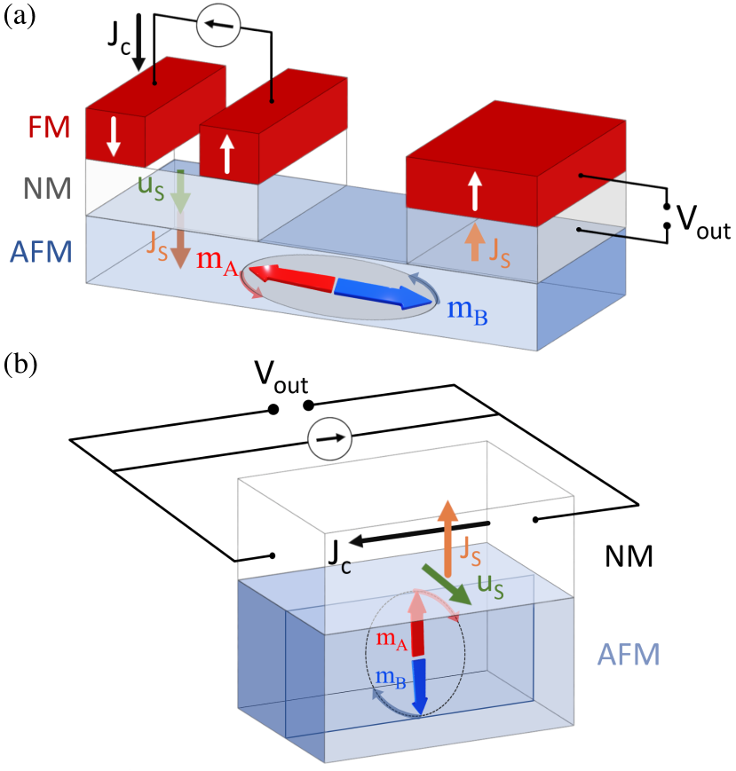
Figure 6: Device setup for electrical control and detection of terahertz oscillations in thin-film antiferromagnetic insulators. (a) In-plane spin valve geometry: lateral spin valve structure made of a perpendicular reference-layer magnetization on top of an in-plane-anisotropy antiferromagnet. (b) Perpendicular spin Hall geometry: spin Hall structure with in-plane electric current transverse to in-plane hard axis on top of a perpendicular-anisotropy antiferromagnet. Input electric current $J_{\text{c}}$ is converted into a pure spin current $J_{\text{s}}$ polarized $\mathbf{u}_{\text{s}}$ along the hard-anisotropy axis to cause precession of the sublattice moments $\mathbf{m}_{A}$ and $\mathbf{m}_{B}$, which pumps spin current back to generate an oscillating voltage signal at the output $V_{\text{out}}$. FM: ferromagnet, NM: normal metal, AFM: antiferromagnet.

For the choice of spin polarization along the hard axis of the antiferromagnetic layer, the viable geometries are the in-plane-anisotropy antiferromagnet with the lateral spin valve structure made of a perpendicular reference-layer magnetization, and the perpendicular-anisotropy antiferromagnet with the spin Hall structure in which the in-plane electric current is transverse to the in-plane hard axis. For both the geometries, the input is a constant-current source, the back diffusion (“backflow”) of injected spins Jiao and Bauer (2013) is considered small, and the output is detected under open-circuit condition.

To excite and control Néel-order precession, the spin current must exert adequate antidamping-like torque. The threshold spin-current density that initiates precession is obtained from the condition $\Gamma_{\text{th}}=1$ (11) as $J_{\text{s,th}}=\mathcal{K}_{\text{e}}d_{\text{a}}/2$. The corresponding electric-current density depends on the specific geometry. For the in-plane spin valve geometry, assuming low spin-memory loss in the normal metal, the conversion from electric current to spin is determined by the conductance of majority and minority-spin electrons $g_{\text{M}}$ and $g_{\text{m}}$, respectively, and the spin-mixing conductance at the interface of normal metal and antiferromagnet $g_{\text{r}}$. The threshold electric-current density is Skarsvåg et al. (2015)

$$J_{\text{c,th}}^{\text{ip-valv}}=\frac{2e}{\hbar}\frac{(g_{\text{r}}+g_{\text{M}}+g_{\text{m}})(g_{\text{M}}+g_{\text{m}})}{g_{\text{r}}(g_{\text{M}}-g_{\text{m}})}J_{\text{s,th}}.$$ (24)

For the perpendicular spin Hall geometry, the conversion from electric current to spin is determined by the spin Hall angle $\Theta_{\text{s}}$, the layer thickness $d_{\text{n}}$, the spin diffusion length $\lambda$ and the conductivity $\sigma$ of the heavy metal, and the spin-mixing conductance at the interface of heavy metal and antiferromagnet $g_{\text{r}}$. The threshold electric-current density is Cheng et al. (2016a)

$$J_{\text{c,th}}^{\text{pe-Hall}}=\frac{e}{\hbar}\frac{\sigma}{\lambda g_{\text{r}}}\frac{\coth{(d_{\text{n}}/2\lambda)}}{\Theta_{\text{s}}}J_{\text{s,th}}.$$ (25)

If the effective damping $\beta\ll 1$, the minimum current for sustaining precession is about $1/\beta$ times lower as seen from Fig. 2 and Eq. (11). Lowering the current drive after initiation mitigates excessive Joule heating in the metal, and allows for tunability of oscillation to sub-terahertz frequencies detectable by microelectronic circuits.

Precessing Néel order can reciprocally pump time-varying spin current $\propto\mathbf{n}\times\mathbf{n}^{\prime}$ back into the adjacent metal, and experience a damping-like backaction Cheng et al. (2014). This virtually enhances the Gilbert damping expressed as $\alpha=\alpha_{0}+\alpha_{\text{s}}$, where $\alpha_{0}$ is the intrinsic damping constant and the enhancement Cheng et al. (2016a)

$$\alpha_{\text{s}}=\frac{\hbar^{2}\gamma g_{\text{r}}}{2e^{2}M_{\text{s}}d_{\text{a}}}.$$ (26)

The pumped spin current is converted into voltage under open-circuit condition via spin filtering for the in-plane spin valve geometry and via inverse spin Hall effect for the perpendicular spin Hall geometry. The voltage signal generated at the output of each geometry is Skarsvåg et al. (2015); Cheng et al. (2016b)

$$V_{\text{out}}^{\text{ip-valv}}(t)=\frac{\hbar\gamma\sqrt{\mathcal{J}\mathcal{K}_{\text{e}}}}{2eM_{\text{s}}}\frac{g_{\text{r}}(g_{\text{M}}-g_{\text{m}})\omega(t)}{(g_{\text{r}}+g_{\text{M}}+g_{\text{m}})(g_{\text{M}}+g_{\text{m}})},$$ (27)

$$V_{\text{out}}^{\text{pe-Hall}}(t)=\frac{\hbar\gamma\sqrt{\mathcal{J}\mathcal{K}_{\text{e}}}}{2eM_{\text{s}}}\frac{\lambda g_{\text{r}}}{\sigma}\Theta_{\text{s}}\tanh(\frac{d_{\text{n}}}{2\lambda})\omega(t),$$ (28)

where $\omega$ is the dimensionless angular frequency (Sec. III.1).

Table 1: Properties of bulk NiO and Cr₂O₃ at 300 K

Parameter	NiO	Ref.	Cr2O3	Ref.
$\mathcal{J}$ (J/m3)	$3.4\times 10^{8}$	Sievers III and Tinkham, 1963,Khymyn et al.,2017	$9.5\times 10^{7}$	Parthasarathy and Rakheja, 2019b,Foner,1963
$\mathcal{K}_{\text{e}}$ (J/m3)	$2.2\times 10^{4}$	Sievers III and Tinkham, 1963,Khymyn et al.,2017	$3.2\times 10^{3}$	Parthasarathy and Rakheja, 2019b,Foner,1963
$\mathcal{K}_{\text{h}}$ (J/m3)	$5.5\times 10^{5}$	Sievers III and Tinkham, 1963,Khymyn et al.,2017	$\approx 0$	Parthasarathy and Rakheja, 2019b,Foner,1963
$M_{\text{s}}$ (A/m)	$3.5\times 10^{5}$	Hutchings and Samuelsen, 1972,Khymyn et al.,2017	$1.9\times 10^{5}$	Parthasarathy and Rakheja, 2019b,Foner,1963
$\alpha_{0}$	$6\times 10^{-4}$	Hutchings and Samuelsen, 1972,Khymyn et al.,2017	$2\times 10^{-4}$	Parthasarathy and Rakheja, 2019b,Samuelsen et al.,1970

Table 2: Characteristics of device geometry

Parameter	Layer info	Ref.
$g_{\text{M}}=10^{10}$ (S/m2)	NM/FM	Skarsvåg et al.,2015
$g_{\text{m}}=10^{9}$ (S/m2)	NM/FM	Skarsvåg et al.,2015
$g_{\text{r}}=10^{14}$ (S/m2)	NM/AFM	Baldrati et al.,2018
$d_{\text{a}}=5$ nm	AFM	Khymyn et al.,2017
$\sigma=10^{6}$ (S/m)	NM (Pt)	Khymyn et al.,2017
$d_{\text{n}}=20$ nm	NM (Pt)	Khymyn et al.,2017
$\lambda=7$ nm	NM (Pt)	Khymyn et al.,2017
$\Theta_{\text{s}}=0.1$	NM (Pt)	Khymyn et al.,2017

Bipartite collinear antiferromagnets such as NiO and Cr₂O₃ are insulators, whose bulk magnetic properties are well-studied (Table 2). For thin films, density functional theory predicts that NiO(001) on SrTiO₃ substrate has an in-plane anisotropy Chen et al. (2018), and experiments have shown that Cr₂O₃(0001) on Al₂O₃ substrate has a perpendicular anisotropy Wu et al. (2011), but measurement of magnetic anisotropy of antiferromagnetic films is less explored Jungwirth et al. (2018). The magnetic anisotropy of thin films and multilayers can significantly differ from bulk magnetic materials due to epitaxial strain from substrate and reduced local symmetry of surface atoms Sander (2004). The magnetic anisotropy energy is augmented by magnetostrictive and surface anisotropies which can elicit an in-plane or a perpendicular spin orientation independent of the specific growth direction of the film Krishnan (2016). Nonetheless, we consider the bulk properties to estimate specifications for the proposed setup.

For characteristic values of geometry parameters (Table 2), the threshold current density $J_{\text{c,th}}^{\text{ip-valv}}\approx 2\times 10^{7}$ A/cm² and $J_{\text{c,th}}^{\text{pe-Hall}}\approx 10^{8}$ A/cm²; the effective damping $\beta^{\text{ip-valv}}=0.18$ and $\beta^{\text{pe-Hall}}=0.24$; the frequency scale is 1.4 THz for NiO and 0.5 THz for Cr₂O₃; the amplitude of alternating output signal $v_{\text{out}}^{\text{ip-valv}}=70$ µV and $v_{\text{out}}^{\text{pe-Hall}}=0.4$ µV at the threshold current . The specifications are promising for practical demonstration of a terahertz signal emitter at nanoscale lengths.

Additionally, the setup can detect a terahertz radiation by phase-locking if the antiferromagnet’s crystal symmetry allows for staggered-field Néel spin-orbit torque, which includes materials such as CuMnAs and Mn₂Au Gomonay et al. (2018). By changing the spin polarization angle and the threshold spin-current density from $2J_{\text{s,th}}/d_{\text{a}}\propto\alpha\sqrt{\mathcal{J}\mathcal{K}_{\text{e}}}$ to $\mathcal{K}_{\text{e}}+\mathcal{K}_{\text{h}}$ (22), hence the precession axis, the minimum angular frequency $\omega_{0}$ can be tuned from zero to $\sqrt{\kappa+1}$. This method proportionally shifts the center of the phase-locking interval. Frequencies below $\omega_{0}$ are cut off and this system acts as a high-pass filter operating in the terahertz range.

V Conclusion

We study the equation of motion of the Néel order of an antiferromagnet under the action of spin torque for steady-state solution, which involves precession in a circular orbit about an axis oriented along a general direction. The required components of the spin-polarization vector in the orbital plane are explicit functions of the axis orientation. We analyze the dynamics by bisecting it into angular motion in the orbit and perturbation from the orbital plane.

The angular motion reduces to equation of a damped-driven pendulum described by two parameters which represent the effective damping and drive. The parameter space is explored to identify regions of periodicity, hysteresis and infinite-period bifurcation. Solutions for oscillations in angular velocity are derived when the damping and drive are separately large, and a function for the fundamental frequency is found. The oscillations are sinusoidal for large drive and spike-like for large damping near threshold.

The perturbing elevation from the orbital plane reduces to equation of a damped harmonic oscillator with an effective spring constant. The stability condition introduces a minimum cutoff frequency for orbits, using which the threshold spin current is calculated. Orbital axes which deviate sufficiently from the hard axis have nonzero cutoff frequency, increasing monotonically with highest value for the easy-axis direction. The threshold is lowest along the hard axis, which varies non-monotonically with the angle from the hard axis for small damping.

Finally, we propose device setups for electrical control and detection of terahertz oscillations in thin-film antiferromagnets. A certain practical challenge in achieving arbitrary precessional axis orientations is generating adequate spin-current density that overcomes the threshold, or reducing the magnetic anisotropy by strain-engineering to lower the current requirement.