Predicting Urban Innovation from the Workforce Mobility Network in US

Abstract

While great emphasis has been placed on the role of social interactions as driver of innovation growth, very few empirical studies have explicitly investigated the impact of social network structures on the innovation performance of cities. Past research has mostly explored scaling laws of socio-economic outputs of cities as determined by, for example, the single predictor of population. Here, by drawing on a publicly available dataset of the startup ecosystem, we build the first Workforce Mobility Network among US metropolitan areas. We found that node centrality computed on this network accounts for most of the variability observed in cities’ innovation performance and significantly outperforms other predictors such as population size or density, suggesting that policies and initiatives aiming at sustaining innovation processes might benefit from fostering professional networks alongside other economic or systemic incentives. As opposed to previous approaches powered by census data, our model can be updated in real-time upon open databases, opening up new opportunities both for researchers in a variety of disciplines to study urban economies in new ways, and for practitioners to design tools for monitoring such economies in real-time.

Introduction

Over the last two decades, developed and developing countries alike have witnessed a radical transformation in the nature and dynamics of their innovation processes. A major factor that has triggered this change is the emergence of new entrepreneurial ecosystems centered on high-growth startups. In the United States, startups account for the majority of new job creations [1] and have rapidly expanded not only in size but also geographically by creating distributed innovation centers [2]. Abundant empirical evidence supports the idea that young and innovative firms guarantee the long-term growth of cities and sustain the economic life by creating wealth and new jobs also in related industries [3, 4, 5, 6, 7, 8].

Researchers have tried to shed light on early indicators of success in modern innovation environments. In the attempt of building baseline models to predict innovation in cities, past efforts have mainly focused on predicting a wide range of socio-economic indicators of wealth (e.g., GDP, employment, housing and infrastructures) and a range of innovation indicators (e.g., abundance of young firms, number of patents granted) [9, 10, 11] solely based on population size or density. These studies have shown that population size alone is able to reliably predict – with a coefficient of determination $R^{2}$ for linear regression in the $[0.88,0.99]$ range – several socio-economic outputs of cities including income, electrical consumption, total wages, and employment. Yet, the correlations between population characteristics and outputs associated with innovation processes such as number of granted patents $(R^{2}=0.72)$, number of inventors $(R^{2}=0.76)$, and R&D establishments $(R^{2}=0.77)$ are not equally strong. In fact, innovation-related indicators report the smallest correlation coefficients among all the other variables [10] (Figure 1).

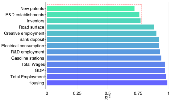
Figure 1: Correlation coefficients between population size and various socio-economic outputs, adapted from L. Bettencourt et. al. [10]. Data suggest that innovation-related indicators (marked in red) are less correlated with population than other socio-economic outputs. These results are computed with data covering the [1997,2003] period.

This discrepancy points to three main limitations of prediction models solely based on demographic variables. First, by treating geographical areas as isolated entities, such models overlook the role of social interactions, yet well-established urban theories[13] and qualitative [15] and quantitative findings in economics [14] have repeatedly shown that a dense and dynamic web of interactions among specialized workers, entrepreneurs, and investors – also referred to as the “thickness of the market” – plays a pivotal role in driving idea recombination, innovation generation, and ultimately economic growth [12, 16, 17]. Second, these past models do not account for the fact that cities grow through the attraction of highly talented individuals (also called ‘the creative class’ [18]), and the creative outputs from such individuals have been recently found to explain super-linear urban scaling [19]. Finally, the life cycle of a modern innovative startup – its birth, growth, acquisition, and extinction – is much faster than the time frames within which past models’ inputs (e.g., demographic data) and outputs (e.g., patenting rates) are typically defined.

Previous research has provided evidence that simple scaling laws of population miss evolutionary dynamics that are key to explain many city-level processes [20], and that the application of tools from statistical physics to a variety of spatial networks allows for a more accurate description of such complex dynamics [21, 22, 23, 24, 25]. However, constrained by limited data availability, only a few empirical studies have attempted to investigate the impact of different types of social network structures on economic growth and innovation performance of cities [9, 26, 27, 28, 29].

This work contributes to fill the gap by drawing on a novel dataset from CrunchBase, an online database containing historical records of the evolution of the worldwide startup ecosystem. From this data, to be able to consider network effects, we built and analyzed the first Workforce Mobility Network (WMN), which, unlike previous approaches in the literature, can be updated in real-time. The network’s nodes are metropolitan areas, and its links (edges) are workforce flows between area pairs (an edge weight is equal to the number of professionals who have worked at companies located in both of the two metropolitan areas the edge connects). Figure 2 provides an illustration of the procedure adopted to construct WMN: Mr. Ramy Majouji quits his job at Square Inc., a company based in the San Francisco-Oakland-Hayward metropolitan area (green), to then join Codecademy, located in the New York-Newark-Jersey area (red), thus acting as a bridge between the two areas; ultimately, the link between the “San Francisco-Oakland-Hayward” node and the “New York-Newark-Jersey” node has a weight equal to the number of unique workers bridging the companies located in the two areas.

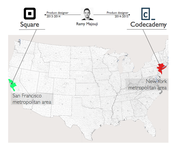
Figure 2: Example of how the Workforce Mobility Network (WMN) is built. Its nodes represent Metropolitan Statistical Areas (MSA) in the United States, while each of its links has a weight equal to the number of employees who worked at the companies located in the two corresponding metropolitan areas. For instance, Ramy Majouji, who moved from Square Inc. in the San Francisco area (green) to Codecademy in the NewYork area (red), acted as a bridge between the two companies and contributed to increase the weight of the link between the two areas by one.

The opportunity to recombine ideas and access relevant knowledge is crucial for companies that aim at generating innovation [30, 31, 32]. The likelihood of a company benefiting from new ideas, know-how, and talents is determined not only by the availability of these resources within the city where the company is located but also by the opportunity to absorb them from other cities. As such, we hypothesized that the most central areas in WMN, rather than the most densely populated ones, are the most innovative. To test our hypothesis, we considered two innovation measures for each metropolitan area $i$: i) the number $\mathcal{S}_{i}$ of successful startups in $i$ (a startup is successful if it either was acquired, did an Initial Public Offering (IPO), or acquired another startup); and ii) the cumulative acquisition price $\mathcal{A}_{i}$ of all startups in $i$. Differently from commonly used measures of output such as the number of granted patents, our measures adapt more dynamically to the rapidly changing market and better reflect a startup’s ability to translate its innovation potential into immediate and tangible economic value. In a modern innovation landscape characterized more and more by digital solutions, global outreach, low barrier to entries, and extremely fast business developments, the number of patents might not fully reflect actual levels of innovation. Often patents are used as a defensive tool against ‘patent trolling’ [33] or are used to discourage the entry of market newcomers rather than actually being used to produce and commercialize genuinely innovative products [34]. For completeness, we present empirical results considering patenting rates as a proxy for innovation as well, and do so in the Supplementary Material.

In summary, we measured to which extent WMN – specifically, the centrality of its nodes – predicts innovation performance of cities, measured through $\mathcal{S}_{i}$ and $\mathcal{A}_{i}$, and how those predictions compare to previous models’ in the literature.

Results

All the following models are based on startups that were active in the United States in 2010, and on all their historical information up to that year. For each of the metropolitan areas in which these startups were located, we measured the innovation performance indicators $\mathcal{S}_{i}$ and $\mathcal{A}_{i}$ in the [2010-2016] period.

Residual variability of population-based models

Consistently with previous work [10], we found a non-linear scaling of our two innovation measures $\mathcal{S}_{i}$ and $\mathcal{A}_{i}$ with population size $\mathcal{P}_{i}$, and with past fundings $\mathcal{F}_{i}$ (Figure 3).

However, despite the correlations being strong, performance variability is still high. Many cities that are similar in size and in past fundings expressed very different performances. For example, the North Port-Bradenton-Sarasota metropolitan area (Florida) and the Colorado-Springs metropolitan area (Colorado) are very similar with respect to number of startups active in 2010 (respectively $106$ and $99$), population ($\sim 10^{6}$), and funding received ($\sim 10^{8}\$$), yet the performances of their companies are significantly different: companies in “North Port-Bradenton-Sarasota” have been sold for a cumulative value of $5.8\cdot 10^{9}\$$, while those in “Colorado-Springs” reported a cumulative acquisition price smaller by two orders of magnitude, namely $4.3\cdot 10^{7}\$$.

Our aim was to investigate to which extent these differences in performance could be accounted for by other predictors. In particular, we hypothesized that workforce mobility explains most of the residual variability.

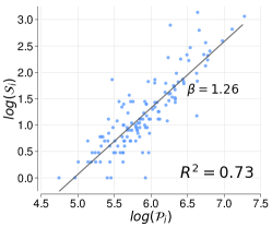
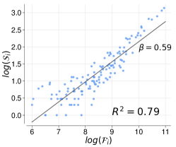
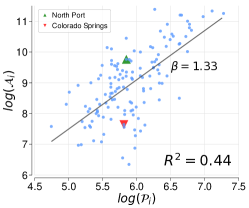
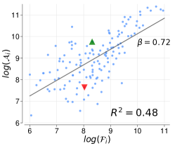
Figure 3: Scatter plots of our two innovation measures, namely the total number of successful startups $\mathcal{S}_{i}$ and the cumulative acquisition price $\mathcal{A}_{i}$, against population size $\mathcal{P}_{i}$ and total past fundings $\mathcal{F}_{i}$. Double logarithmic plots, coefficients of determination $R^{2}$, and corresponding $\beta$-coefficients for the four least-square linear regressions are shown.

The Workforce Mobility Network

We constructed the Workforce Mobility Network (WMN) among metropolitan areas by using CrunchBase job records for all startups active up to the year of 2010. Among the 380 metropolitan areas in the United States, $243$ had at least one active startup in our data. As a result, the final network had $243$ nodes and $2,169$ edges, and reflected $26,660$ worker flows among metropolitan areas. The maximum node degree is 165, and the maximum node strength (the maximum sum of the link weights for a node) is 8,370. The strength distribution follows a power-law function with an exponent $\sim 2$, a value similar to those observed in other real-world weighted networks [35].

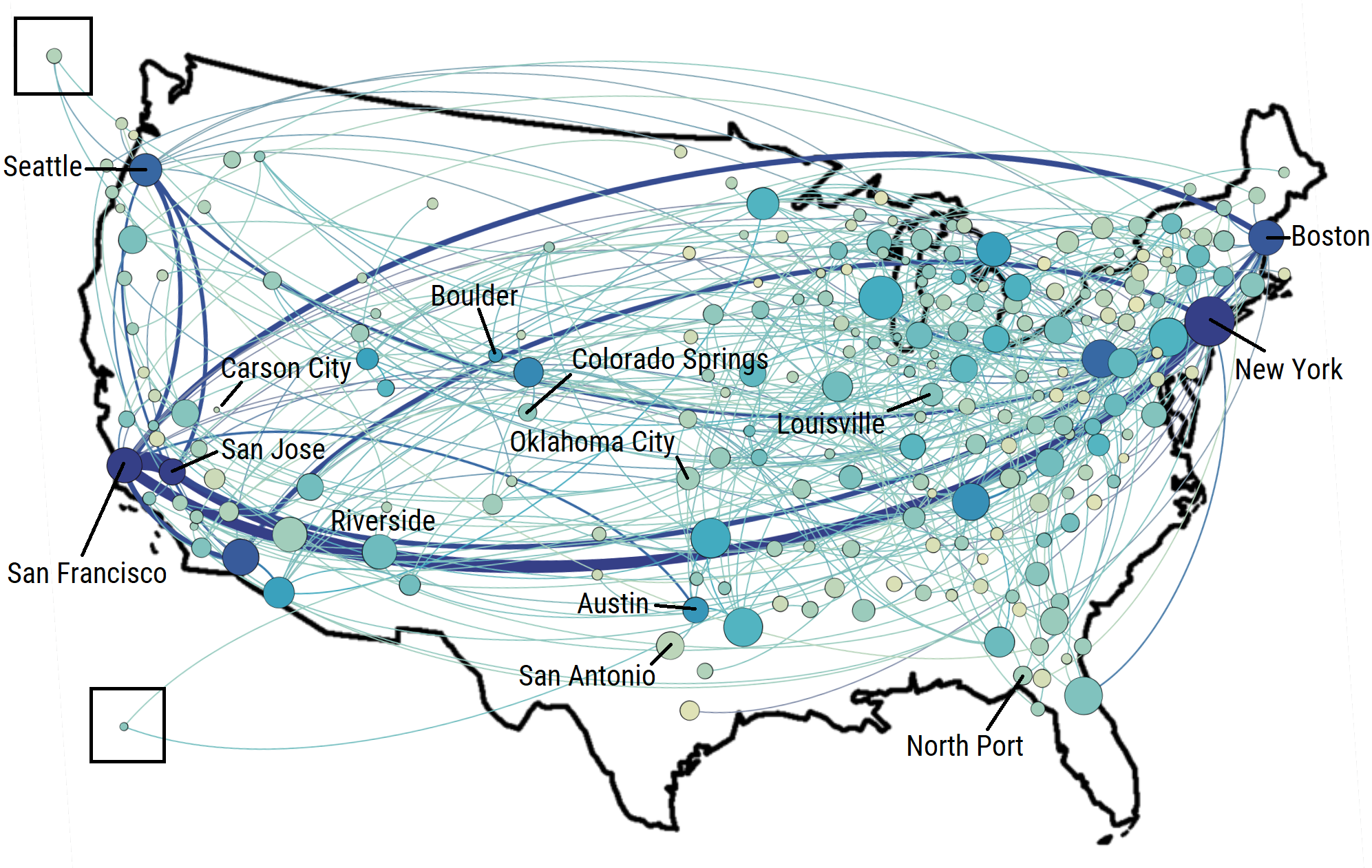
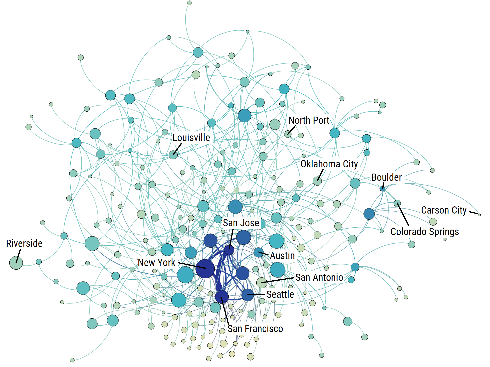
Figure 4: The backbone of the Workforce Mobility Network (WMN) visualized: (A) on the map of the United States; and (B) on a standard force-directed network layout. A node’s size is proportional to the area’s population size, its color intensity is proportional to its PageRank centrality, and an edge’s width is proportional to its weight.

To visualize WMN, we projected it onto the map of the United States, centering its nodes on the metropolitan areas they represent (Figure 4A). Since the number of edges was high, to improve the visualization, we reduced the number of displayed edges with a network backbone extraction algorithm [36], which identified the most statistically significant edges for each node and pruned the rest out. We then computed each node’s centrality according to four measures (see Methods), and PageRank yielded the best fit. In Figure 4, we notice that the most central nodes tend to be US coastal areas, which happen to be linked with each other by the strongest edges. Although population and centrality are in general well correlated (Spearman rank correlation $\rho=0.70$), large fluctuations are still observed: indeed, despite being large, several cities do not score high in terms of node centrality (Figure 4B).

To identify cities that are small yet central, and viceversa, we ranked cities by their ratios $\eta$ between their PageRank centrality values $C_{i}^{PR}$ and their population sizes $\mathcal{P}_{i}$:

$$\eta=\frac{C_{i}^{PR}/\sum_{j}{C_{j}^{PR}}}{\mathcal{P}_{i}/\sum_{j}{\mathcal{P}_{j}}}.$$ (1)

Both centrality values and population sizes are normalized by their sums across all areas. Table 1 shows the 10 metropolitan areas with the highest values of $\eta$, and the 10 with the lowest values. Metropolitan areas at the top have higher centrality relative to their population size. These include large and central areas such as San Francisco as well as much smaller cities (e.g., Boulder and Ithaca) that are remarkably central despite their limited size. On the other hand, the ten cities at the bottom are very populous yet not central in workforce flows, and, with the exception of Virginia Beach, the remaining nine cities experience relatively limited financial returns from innovation. These findings seem to suggest that network centrality might predict innovation performance better than what population counts would do. We set out to test that proposition next.

Top 10 according to $\eta$				Bottom 10 according to $\eta$
MSA	Population	Price $\mathcal{A}_{i}$	$\eta$	MSA	Population	Price $\mathcal{A}_{i}$	$\eta$
San Jose CA	1.8M	245B	8.20	Riverside CA	4.2M	315M	0.161
San Francisco CA	4.3M	160B	6.74	Oklahoma City OK	1.2M	648M	0.262
Boulder CO	0.3M	1.7B	5.14	Fresno CA	1.0M	30M	0.445
Boston MA	4.5M	159B	4.82	Virginia Beach VA	1.7M	4.7B	0.446
Springfield MO	0.4M	0.3B	4.73	Louisville KY	1.3M	229M	0.464
Cedar Rapids IA	0.3M	0.3B	4.42	Buffalo NY	1.1M	27M	0.468
Carson City NV	0.1M	38M	3.92	San Antonio TX	2.1M	278M	0.469
Seattle WA	3.4M	32B	3.88	Columbia SC	0.8M	2M	0.470
Austin TX	1.7M	14B	3.77	Birmingham AL	1.1M	169M	0.471
Ithaca NY	0.1M	0.5B	3.71	Sacramento CA	2.2M	981M	0.489

Table 1: Cumulative acquisition prices $\mathcal{A}_{i}$ for the ten metropolitan areas (MSAs) with the highest values of centrality/population ratio $\eta$, and the ten cities with the lowest values.

Predicting innovation performance of cities

We used linear regression to evaluate the impact of demographic characteristics and network characteristics on the performance of an area’s startups. Linear regression is an approach for modeling a linear relationship between a dependent variable (our innovation measure $\mathcal{S}_{i}$ or $\mathcal{A}_{i}$) and a set of independent variables, and it does so by associating a so-called $\beta$-coefficient with each independent variable such as the sum of all independent variables multiplied by their respective $\beta$-coefficients approximates the value of the dependent variable with minimal error. Specifically, we used an ordinary least square (OLS) regression model to estimate the coefficients such that the sum of the squared residuals between the estimation and the actual value is minimized. In line with what discussed by Bettencourt et al. [38], it is more appropriate to express the dependent variable using absolute values (i.e., number of successful startups, total acquisition prices) rather than using ratios (e.g., percentage of successful startups) or per-capita values. That is because these two latter quantities implicitly assume that the dependent variable (e.g., innovation measure) linearly increases with the independent variables (e.g., number of existing startups, population size), while we know that it tends to super-linearly increase with them.

In the regression models, we experimented with two different groups of predictors: i) socio-economic indicators; and ii) indicators based on WMN’s structure. First, the socio-economic indicators based on the literature are population size [10], population density [12], and number of patents granted in each metropolitan area up to 2010 [9]. To those three indicators, we added two others derived from CrunchBase: the number of active startups $\mathcal{N}_{i}$ in 2010, and the total past funding $\mathcal{F}_{i}$ raised up to the year of 2010. The number of active startups $\mathcal{N}_{i}$ is an upper bound for the number of successful ones and, as such, represents an important variable to control for; on the other hand, the independent variable of past funding $\mathcal{F}_{i}$ is not necessarily correlated with our dependent variable (i.e., with the actual innovation levels of companies), can be influenced by factors such as local tax policies, and, as such, can be regarded as a proxy for innovation incentives each area tends to enjoy.

Second, the indicators based on WMN’s structure aim at capturing each area’s centrality in the flows of ideas, techniques, knowledge, creative inputs, and business opportunities [39]. To characterize the potential exposure of a metropolitan area to these flows, we computed four centrality measures: degree centrality, node strength, Google PageRank, and harmonic closeness (see Methods). The node degree and the node strength are local measures that estimate the potential of an area to exchange resources with its immediate neighbors, while the latter two are global measures. The PageRank score of a node is proportional to the number of “random walkers” who happen to traverse that node at stationary state[40]. If we imagine knowledge as a collection of discrete units and assume that these units randomly flow in WMN, then an area’s PageRank score is the fraction of the global knowledge the area has potential access to (e.g., if the score is 0.2, then 20% of the global knowledge is potentially accessible by the area). In a similar way, area $i$’s harmonic closeness is the distance (measured as the weighted number of hops) that a given unit of information needs to traverse to reach node $i$ starting from any other node [41, 42, 43, 44].

Table 2 reports the adjusted coefficients of determination $R^{2}$ and the $\beta$-coefficients for the ten models. The first 9 models consider the independent variables separately. We see that predicting acquisition prices $\mathcal{A}_{i}$ is harder than predicting the number of successful startups $\mathcal{S}_{i}$, yet the relative powers of the predictors are mostly consistent across the two innovation measures. All the socio-economic indicators (models 1–5) are good predictors, and, among them, the control variable of the number of active startups (5) is the most powerful, with $R^{2}=0.96$ for $\mathcal{S}_{i}$, and $R^{2}=0.76$ for $\mathcal{A}_{i}$, not least because the number of active startups is an upper bound for the number of successful ones. In line with previous empirical findings [10], population (1) is positively correlated with both innovation measures. However, population density (2) is less so. Past fundings (3) and number of patents (4) are also positively associated, yet have the smallest $\beta$-coefficients. The last four models (models 6–9) test our four network centrality measures: PageRank (6) and node strength (7) have higher $\beta$-coefficients and $R^{2}$ compared to node degree (8) and harmonic centrality (9), which do not account for network weights (that is, for the extent to which global knowledge tends to be accessible by each area). Overall, PageRank outperforms population by $12\%$ when predicting $\mathcal{S}_{i}$, and by $27\%$ when predicting $\mathcal{A}_{i}$.

To further disentangle the unique contribution of each predictor, we used a stepwise feature selection procedure (see Methods for details) to select the combination of predictors with the highest $R^{2}$. The two models that consist of the selected variables are reported in the last columns of the two panels in Table 2 (columns 10). PageRank is the only network metric retained by the feature selection method because it is the only one that, in combination with the socio-economic features, improves the overall prediction. Also, the $\beta$-coefficient of PageRank is the highest for $\mathcal{A}_{i}$, and the second highest (only after the control variable of the number of active startups) for $\mathcal{S}_{i}$. In both cases, the coefficients of determination are significantly larger than those obtained for the other variables, especially than those obtained for population size and density.

In multivariate regressions, if the independent variables are perfectly independent, then the coefficient of determination $R^{2}$ decomposes itself into the sum of the squares of the Pearson’s correlation coefficients computed for each variable separately. However, in our case, as in the majority or real-world scenarios, most of the variables are correlated with each other, and the sum of each independent $R^{2}$ exceeds the one obtained for the multivariate regression (model 10). To properly decompose the relative contribution of the correlated independent variables, we used the LGM method [45] and computed the relative importance of each predictor (Figure 5). Interestingly, after controlling for the number of active startups, PageRank is confirmed to be the predictor that explains most of the variability in the data.

	Dependent variable: number of successful startups $\mathcal{S}_{i}$
	(1)	(2)	(3)	(4)	(5)	(6)	(7)	(8)	(9)	(10)
Population	0.853∗∗∗									0.087∗
	(0.046)									(0.050)
Pop. density		0.627∗∗∗								0.050∗
		(0.068)								(0.028)
Funding raised			0.890∗∗∗							0.164∗∗∗
			(0.040)							(0.048)
Patents				0.862∗∗∗
				(0.044)
Active startups					0.961∗∗∗					0.511∗∗∗
					(0.024)					(0.084)
Network PageRank						0.907∗∗∗				0.222∗∗∗
						(0.037)				(0.049)
Network strength							0.911∗∗∗
							(0.036)
Network degree								0.871∗∗∗
								(0.043)
Harmonic centrality									0.751∗∗∗
									(0.058)
Constant	$-$0.000	0.000	0.000	$-$0.000	$-$0.000	$-$0.000	$-$0.000	$-$0.000	$-$0.000
	(0.045)	(0.068)	(0.040)	(0.044)	(0.024)	(0.037)	(0.036)	(0.043)	(0.057)	(0.021)
Adjusted R2	0.73	0.39	0.79	0.74	0.92	0.82	0.83	0.76	0.56	0.94

	Dependent variable: cumulative acquisitions prices $\mathcal{A}_{i}$
	(1)	(2)	(3)	(4)	(5)	(6)	(7)	(8)	(9)	(10)
Population	0.668∗∗∗									0.153∗
	(0.065)									(0.091)
Pop. density		0.471∗∗∗
		(0.077)
Funding raised			0.698∗∗∗
			(0.063)
Patents				0.715∗∗∗						0.254∗∗
				(0.061)						(0.101)
Active startups					0.758∗∗∗
					(0.057)
Network PageRank						0.748∗∗∗				0.431∗∗∗
						(0.058)				(0.098)
Network strength							0.719∗∗∗
							(0.061)
Network degree								0.673∗∗∗
								(0.065)
Harmonic centrality									0.587∗∗∗
									(0.071)
Constant	0.000	0.000	0.000	0.000	0.000	0.000	0.000	0.000	0.000	0.000
	(0.065)	(0.077)	(0.062)	(0.061)	(0.057)	(0.058)	(0.060)	(0.064)	(0.070)	(0.055)
Adjusted R2	0.44	0.22	0.48	0.51	0.57	0.56	0.51	0.45	0.34	0.6
	∗p$<$0.1; ∗∗p$<$0.05; ∗∗∗p$<$0.01

Table 2: Standardized $\beta$-coefficients of the regression models to predict the two dependent variables of innovation performance, namely the number of successful startups $\mathcal{S}_{i}$ and the cumulative acquisition price $\mathcal{A}_{i}$. Standard errors for the coefficients are reported in parenthesis.

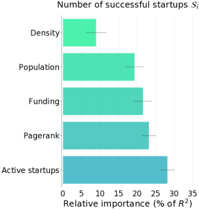
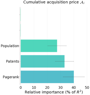
Figure 5: Relative contribution of each variable to the total variance explained by the regression models in Table 2. The relative contribution is expressed as percentage of the $R^{2}$ determined by each variable.

Discussion

This is the first study that has built a Workforce Mobility Network at the scale of an entire country from open data, and that has shown that this network’s structural characteristics are powerful predictors of urban innovation. It turns out that startups benefit from being located in areas that are central in workforce flows: indeed, global network measures tend to predict long-term innovation better than even what cumulative investments do.

Our study comes with limitations that are mostly determined by our data. No sufficient longitudinal data was available for testing causal relationships. Furthermore, startups do not have to publicly disclose their funding rounds or acquisition prices: 83% of the funding rounds in our dataset, for example, have been fully disclosed on CrunchBase. Yet, being of random nature, such missing data has little impact on our two innovation measures, and no impact on a comparative evaluation of areas.

Methods

Datasets

We combined data from three sources. First, from US census data, we extracted information about population size, land area, and population density at the level of Metropolitan Statistical Area (MSA). Second, from the United States Patent and Trademark Office (USPTO), we associated the numbers of patents granted in the year of 2010 with the inventors’ metropolitan areas. Third, from the CrunchBase web APIs, we collected all information regarding organizations and people (workers). For each organization we extracted data on: address of the headquarter, foundation date, funding rounds, acquisitions (also referred to as exits), initial public offers (IPOs), status (active, closed), and team members. The address, in turn, consists of street name, zip-code, city name, and state. Funding rounds record the financial investment of individuals or venture capital firms into a company (organization), i.e., the purchase of a certain percentage of ownership of the company, while acquisitions indicate the transfer of the company’s total ownership to another company. The data on funding rounds and acquisitions include the parties involved, the date, and the monetary value of the transaction in US dollars. We were able to associate the companies in our data with 369 (out of the 374) metropolitan areas. Workers are linked to organizations through the professional roles they hold. Examples of role titles are CEO, founder, board member, and employee. Workers can have multiple jobs/roles within the same organization or across different organizations. About 42% of all the job records include a starting date allowing for a longitudinal analysis of the flow of workers between various firms.

Centrality measures

Different measures of centrality have been proposed over the years to quantify the importance of a node in a complex network [35]. In this work, we computed four centrality measures for each WMN node: degree centrality, node strength, harmonic closeness, and Google PageRank.

Let $G$ be a weighted graph with $N$ nodes described by the $N\times N$ weighted adjacency matrix $W=\{w_{ij}\}$ whose entry $w_{ij}$ is equal to the weight of the link connecting node $i$ to node $j$, or is equal to $0$ if the nodes $i$ and $j$ are not connected. As for the case of $G$ being an unweighted graph, we define the adjacency matrix $A=\{a_{ij}\}$ of $G$, which simply indicates which pairs of nodes are connected with a $N\times N$ matrix such that $a_{ij}=1$ if $w_{ij}\neq 0$, and $a_{ij}=0$ if $w_{ij}=0$.
Our first centrality measure out of the four is degree centrality, which is based on the idea that important nodes are those with the largest number of ties to other nodes in the graph. The degree centrality of node $i$ is defined as:

$$C^{D}_{i}=\frac{k_{i}}{N-1}=\frac{\sum_{j={1}}^{N}a_{ij}}{N-1}$$ (2)

where $k_{i}$ is the degree of node $i$.
Our second centrality measure is strength centrality. For each node $i$, this is defined as:

$$C^{S}_{i}=\frac{s_{i}}{\sum_{j}s_{j}}=\frac{\sum_{j={1}}^{N}w_{ij}}{\sum_{i,j}w_{ij}}$$ (3)

where strength $s_{i}$ of node $i$ is the sum of the weights of the edges incident in $i$.
Our third centrality measure is the harmonic closeness centrality [42]. For each node $i$, it measures its minimum distance or geodesic $d_{ij}$ to another node $j$, i.e., the minimum number of edges traversed to get from $i$ to $j$:

$$C^{C}_{i}=\sum_{j}\frac{1}{d_{ij}}.$$ (4)

Our fourth and final centrality measure is the PageRank centrality. For each node $i$, this is the stationary probability that a “surfer” that randomly travels on the network’s links arrives at node $i$. It is recursively defined as:

$$C^{PR}_{i}=\frac{1-\alpha}{N}+\alpha\cdot\sum_{\{j|(i,j)\in A\}}\frac{C^{PR}_{j}}{k_{j}}$$ (5)

where $k_{j}$ is the degree of node $j$, and $\alpha$ is a damping factor (traditionally set to 0.85) that models the probability of the surfer following an existing link instead of jumping to any other node picked at random with uniform probability. In this work, we considered a weighted version [47] of the PageRank centrality that sets the probability of following a link proportional to the weight of that link. Formally, this is expressed as:

$$C^{PR}_{i}=\frac{1-\alpha}{N}+\alpha\cdot\sum_{\{j|(i,j)\in A\}}C^{PR}_{j}\cdot\frac{w_{ji}}{s_{j}}$$ (6)

where the factor $\frac{w_{ji}}{s_{j}}$ expresses the probability of transitioning from node $j$ to node $i$ being equal to the weight of the link between $j$ and $i$ ($w_{ji}$) divided by the total strength of node $j$ ($s_{j}$). The PageRank values are computed with an iterative procedure (implemented efficiently through the so-called power method [48]) that starts by assigning a uniform PageRank value to all nodes $C^{PR}_{i}=1/N$, and runs until convergence.

For all the four centrality measures, we considered their normalized versions $\hat{C_{i}}=\frac{C_{i}}{\sum_{j=1}^{N}C_{j}}$ such that the sum of centrality scores over all the nodes in the network is equal to 1.

Regression

Since all regression variables had skewed distributions, we log-transformed them using base-10 logarithm, with the only exception of the harmonic closeness centrality. To appropriately compare the $\beta$-coefficients, we standardized all regression variables. Given a regressor $x$, its standardised version $\tilde{x}$ is given by: $\tilde{x}=(x-\mu)/\sigma$, where $\mu$ is the average value of the variable $x$ in the sample, and $\sigma$ its standard deviation. Feature selection in the last model (model 10) was performed with the feature selection procedure stepAIC implemented in the R standard packages. To estimate the relative feature importance, we used the implementation of the LGM method provided in R in the package relaimpo [49].

Data Availability

All the datasets used in this work can be fully and freely downloaded from the Web. The CrunchBase data is available through its public API at https://data.CrunchBase.com, patent data can be downloaded from http://www.patentsview.org/download, and US census data from https://www.census.gov. To map CrunchBase firms to metropolitan areas, we used the census data available here: https://www.census.gov/geo/maps-data/data/relationship.html.

Supplementary information

Patents granted as outcome variable in the regressions

We constructed several linear regression models to assess the relative contribution of various predictors (population, number of patents, population density, network metrics) in explaining the variability in city’s innovation performance. As a measure of city performance (dependent variable) we have proposed two indicators that directly account for the economic value produced by the start-up firms based in a given city. To compare our results more directly with previous work [9], we also considered patents granted in year 2010 as alternative performance measure (Tab. 3). Also in this case, network features are better predictors than population or population density. In this case, the feature selection indicates network strength as the strongest network predictor which, jointly with funding raised and number of active startups, reaches an $R^{2}$ of $0.79$.

	Dependent variable: patents granted
	(1)	(2)	(3)	(4)	(5)	(6)	(7)	(8)
Population	1.129∗∗∗
	(0.084)
Pop. density		1.117∗∗∗
		(0.140)
Funding raised			0.551∗∗∗					0.157∗∗∗
			(0.032)					(0.058)
Active start-ups				0.941∗∗∗				0.458∗∗∗
				(0.046)				(0.125)
Network PageRank					1.062∗∗∗
					(0.070)
Network strength						0.693∗∗∗		0.211∗∗∗
						(0.037)		(0.086)
Harmonic centrality							0.984∗∗∗
							(0.080)
Constant	-3.908∗∗∗	7.108∗∗∗	-1.863∗∗∗	0.848∗∗∗	5.615∗∗∗	1.632∗∗∗	0.004	0.167∗∗∗
	(0.065)	(0.077)	(0.062)	(0.061)	(0.057)	(0.058)	(0.060)	(0.064)
Adjusted R2	0.58	0.32	0.69	0.76	0.63	0.73	0.53	0.79
	∗p$<$0.1; ∗∗p$<$0.05; ∗∗∗p$<$0.01

Table 3: Standardised beta coefficients of the regression models to predict number of patents granted in 2010. Standard errors of the coefficients are reported in parenthesis.

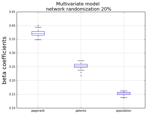
Figure 6: Regression model to predict the cumulative acquisition price $\mathcal{A}_{i}$: distributions of beta coefficients over 100 simulations where $20\%$ of the overall link weight is reduced at random.

Robustness of results to data sparsity

Even though the CrunchBase dataset is, to date, the largest open dataset that tracks job mobility across start-ups, it does not include the full information on mobility. To investigate how much sparsity of the data entries might affect our results and their interpretation, we simulated a scenario where random job entries are dropped and checked whether the relative importance of the predictive variables remain stable. We decreased the overall weight of links in the network by $20\%$, selecting affected links at random and removing them when their strength was reduced to 0. We then run a regression model to predict the cumulative acquisition price $\mathcal{A_{i}}$ using PageRank, number of patents, and population (the three varibles picked by stepwise feature selection). The distributions of the beta coefficients over 100 random simulations (Fig. 6) reveals that the relative weight the coefficient does not change compared to the model that uses all the available data: PageRank has a much higher predictive power than population.

Author contributions statement

MB conducted the experiments and analysed the results. All authors conceived the experiments and contributed to write the manuscript.

References

- [1] Decker, R., Haltiwanger, J., Jarmin, R. & Miranda, J. The role of entrepreneurship in us job creation and economic dynamism. \JournalTitleThe Journal of Economic Perspectives 28, 3–24 (2014).
- [2] Acs, Z. J. & Mueller, P. Employment effects of business dynamics: Mice, gazelles and elephants. \JournalTitleSmall Business Economics 30, 85–100 (2008).
- [3] Mumford, L. The city in history: Its origins, its transformations, and its prospects, vol. 67 (Houghton Mifflin Harcourt, 1961).
- [4] Hall, P. G. & Raumplaner, S. Cities in civilization (Pantheon Books New York, 1998).
- [5] Glaeser, E. L., Rosenthal, S. S. & Strange, W. C. Urban economics and entrepreneurship. \JournalTitleJournal of Urban Economics 67, 1–14 (2010).
- [6] Bos, J. W. & Stam, E. Gazelles and industry growth: a study of young high-growth firms in the netherlands. \JournalTitleIndustrial and Corporate Change 23, 145–169 (2013).
- [7] Haltiwanger, J., Jarmin, R. S. & Miranda, J. Who creates jobs? small versus large versus young. \JournalTitleReview of Economics and Statistics 95, 347–361 (2013).
- [8] Weins, J. & Jackson, C. The importance of young firms for economic growth. \JournalTitleEntrepreneurship Policy Digest (2014).
- [9] Bettencourt, L. M., Lobo, J. & Strumsky, D. Invention in the city: Increasing returns to patenting as a scaling function of metropolitan size. \JournalTitleResearch Policy 36, 107–120 (2007).
- [10] Bettencourt, L. M., Lobo, J., Helbing, D., Kühnert, C. & West, G. B. Growth, innovation, scaling, and the pace of life in cities. \JournalTitleProceedings of the national academy of sciences 104, 7301–7306 (2007).
- [11] Arcaute, E. et al. Constructing cities, deconstructing scaling laws. \JournalTitleJournal of The Royal Society Interface 12, 20140745 (2015).
- [12] Jacobs, J. The death and life of great American cities (Vintage, 1961).
- [13] Jacobs, Jane The Economy of Cities (Vintage, 1970).
- [14] Glaeser, Edward Triumph of the City: How Urban Spaces Make Us Human (Pan Macmillan, 2011).
- [15] Saxenian, A.L. Regional Advantage: Culture and Competition in Silicon Valley and Route 128, With a New Preface by the Author (Harvard University Press, 1996).
- [16] Glaeser, E. & Scheinkman, J. Measuring social interactions. In Durlauf, S. N. & Young, H. P. (eds.) Social dynamics, chap. 4, 83–132 (Boston, MA: MIT Press, 2001).
- [17] Moretti, E. The new geography of jobs (Houghton Mifflin Harcourt, 2012).
- [18] Florida, R. Cities and the creative class (Routledge, 2005).
- [19] Keuschnigg, M., Mutgan, S. & Hedström, P. Urban scaling and the regional divide. \JournalTitleScience Advances 5 (2019).
- [20] Depersin, J. & Barthelemy, M. From global scaling to the dynamics of individual cities. \JournalTitleProceedings of the National Academy of Sciences 115, 2317–2322 (2018).
- [21] Lämmer, S., Gehlsen, B. & Helbing, D. Scaling laws in the spatial structure of urban road networks. \JournalTitlePhysica A: Statistical Mechanics and its Applications 363, 89–95 (2006).
- [22] Barthelemy, M. The structure and dynamics of cities (Cambridge University Press, 2016).
- [23] Kirkley, A., Barbosa, H., Barthelemy, M. & Ghoshal, G. From the betweenness centrality in street networks to structural invariants in random planar graphs. \JournalTitleNature communications 9, 2501 (2018).
- [24] Barbosa, H. et al. Human mobility: Models and applications. \JournalTitlePhysics Reports 734, 1–74 (2018).
- [25] Barthelemy, M. The statistical physics of cities. \JournalTitleNature Reviews Physics 1, 406–415 (2019). DOI 10.1038/s42254-019-0054-2.
- [26] Powell, W. W., Koput, K. W. & Smith-Doerr, L. Interorganizational collaboration and the locus of innovation: Networks of learning in biotechnology. \JournalTitleAdministrative science quarterly 116–145 (1996).
- [27] Makarem, N. P. Social networks and regional economic development: the los angeles and bay area metropolitan regions, 1980–2010. \JournalTitleEnvironment and Planning C: Government and Policy 34, 91–112 (2016).
- [28] Sorenson, O. & Stuart, T. E. Syndication networks and the spatial distribution of venture capital investments1. \JournalTitleAmerican journal of sociology 106, 1546–1588 (2001).
- [29] Eagle, N., Macy, M. & Claxton, R. Network diversity and economic development. \JournalTitleScience 328, 1029–1031 (2010).
- [30] Parise, S., Whelan, E. & Todd, S. How twitter users can generate better ideas. \JournalTitleMIT Sloan Management Review 56, 21 (2015).
- [31] Hargadon, A. B. Firms as knowledge brokers: Lessons in pursuing continuous innovation. \JournalTitleCalifornia management review 40, 209–227 (1998).
- [32] Burt, R. S. The social structure of competition. \JournalTitleExplorations in economic sociology 65, 103 (1993).
- [33] Cohen, L., Gurun, U. G. & Kominers, S. D. The growing problem of patent trolling. \JournalTitleScience 352, 521–522 (2016).
- [34] Nicholas, T. Are patents creative or destructive? \JournalTitleAntitrust Law Journal 79, 405 (2014).
- [35] Latora, V., Nicosia, V. & Russo, G. Complex Networks: Principles, Methods and Applications (Cambridge University Press, 2017).
- [36] Coscia, M. & Neffke, F. M. Network backboning with noisy data. In Data Engineering (ICDE), 2017 IEEE 33rd International Conference on, 425–436 (IEEE, 2017).
- [37] Jacomy, M., Venturini, T., Heymann, S. & Bastian, M. Forceatlas2, a continuous graph layout algorithm for handy network visualization designed for the gephi software. \JournalTitlePloS one 9, e98679 (2014).
- [38] Bettencourt, L. M., Lobo, J., Strumsky, D. & West, G. B. Urban scaling and its deviations: Revealing the structure of wealth, innovation and crime across cities. \JournalTitlePloS one 5, e13541 (2010).
- [39] Bonaventura, M. et al. Predicting success in the worldwide startup network. \JournalTitlearXiv:1904.08171 (2019).
- [40] Page, L., Brin, S., Motwani, R. & Winograd, T. The pagerank citation ranking: Bringing order to the web. Tech. Rep., Stanford InfoLab (1999).
- [41] Boldi, P. & Vigna, S. Axioms for centrality. \JournalTitleInternet Mathematics 10, 222–262 (2014).
- [42] Marchiori, M. & Latora, V. Harmony in the small-world. \JournalTitlePhysica A: Statistical Mechanics and its Applications 285, 539–546 (2000).
- [43] Crucitti, P., Latora, V. & Porta, S. Centrality measures in spatial networks of urban streets. \JournalTitlePhys. Rev. E 73, 036125 (2006).
- [44] Pan, R. K. & Saramäki, J. Path lengths, correlations, and centrality in temporal networks. \JournalTitlePhysical Review E 84, 016105 (2011).
- [45] Lindeman, R., Merenda, P. & Gold, R. Introduction to bivariate and multivariate analysis. \JournalTitleScott, Foresman, & Co, New York (1980).
- [46] Guzman, J. & Stern, S. Where is silicon valley? \JournalTitleScience 347, 606–609 (2015).
- [47] Xing, W. & Ghorbani, A. Weighted pagerank algorithm. In Proceedings. Second Annual Conference on Communication Networks and Services Research, 2004., 305–314 (IEEE, 2004).
- [48] Arasu, A., Novak, J., Tomkins, A. & Tomlin, J. Pagerank computation and the structure of the web: Experiments and algorithms. In Proceedings of the Eleventh International World Wide Web Conference, Poster Track, 107–117 (2002).
- [49] Grömping, U. et al. Relative importance for linear regression in r: the package relaimpo. \JournalTitleJournal of statistical software 17, 1–27 (2006).
Acknowledgements
We thank Valerio Ciotti for his help in collecting the data. VL work was funded by the Leverhulme Trust Research Fellowship “CREATE: the network components of creativity and success”.