See Through Smoke: Robust Indoor Mapping with Low-cost mmWave Radar

Abstract.

This paper presents the design, implementation and evaluation of milliMap, a single-chip millimetre wave (mmWave) radar based indoor mapping system targetted towards low-visibility environments to assist in emergency response. A unique feature of milliMap is that it only leverages a low-cost, off-the-shelf mmWave radar, but can reconstruct a dense grid map with accuracy comparable to lidar, as well as providing semantic annotations of objects on the map. milliMap makes two key technical contributions. First, it autonomously overcomes the sparsity and multi-path noise of mmWave signals by combining cross-modal supervision from a co-located lidar during training and the strong geometric priors of indoor spaces. Second, it takes the spectral response of mmWave reflections as features to robustly identify different types of objects e.g. doors, walls etc. Extensive experiments in different indoor environments show that milliMap can achieve a map reconstruction error less than $0.2$m and classify key semantics with an accuracy of $\sim 90\%$, whilst operating through dense smoke.

1. Introduction

Emergency responders are frequently exposed to harsh and dangerous environments, with consequent threat to life. Statistics collected by the Federal Emergency Management Agency (Agency, [n. d.]) report that over a 10-year period in USA, $2,775$ firefighters died on duty. Where there is a need to save and evacuate victims from a burning, collapsed or flooded building, it is vital for emergency responders to have increased situational awareness. In most search and rescue cases this requires, and begins with, making a map of the unknown environment (Dhekne et al., 2019). Rather than relying entirely on firefighters to slowly explore the building, a promising alternative is to use mobile robots to rapidly survey and build the crucial map. Emergency personnel can then be re-localized accurately within the map and key features such as exit routes can be indicated.

State-of-the-art mapping sensors on mobile platforms (e.g., a smartphone or a mobile robot) use optical sensors, such as laser range scanners (lidar) (Surmann et al., 2003), RGB cameras (Gao et al., 2014; Dong et al., 2015) and stereo cameras (Henry et al., 2014) to produce accurate indoor maps. However, not only are optical sensors impaired by the presence of airborne obscurants (e.g., dust, fog and smoke), their use cases are also significantly restricted by poor-illumination (e.g., dimness, darkness and glare). These adverse conditions regularly occur in emergency situations, e.g., dense smoke for firefighting. Acoustic sensor based mapping approaches, such as ultrasonic (Chong and Kleeman, 1999) and microphones (Pradhan et al., 2018; Zhou et al., 2017), are robust to lighting dynamics, but they either suffer from limited sensing range or become ineffective in noisy environments.

The demand of mapping in the above challenging situations motivates us to consider single-chip millimetre wave (mmWave) radar, which has recently emerged as an innovative low-cost, low-power sensor modality in the automotive industry (Instruments, [n. d.]). A key advantage of mmWave radar is its imperviousness to adverse environmental conditions, such as smoke, fog and dust. In the specific case of fire response, mmWave radars can ‘see’ through smoke and help firefighters understand smoke-filled environments where many other optical sensors fail. Compared with the cumbersome lidar or mechanical radar (e.g., CTS350-X (Weston et al., 2018)), single-chip mmWave radars are lightweight and thus more able to fit payloads of micro robots and form factors of mobile or wearable devices.

Despite these advantages, mmWave-based mapping in indoor environments is still under-explored. The main issues lie in the strong indoor multi-path reflections as well as the sparse measurements returned by single chip radars. In extreme cases, we observe up to $75\%$ outliers due to multi-path reflections, along with more than two orders of magnitude lower point density than a lidar counterpart.

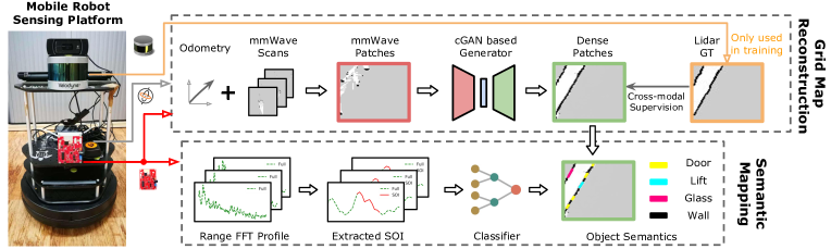
Figure 1. System overview of milliMap, comprising of (1) mobile robotic sensing (2) map reconstruction (3) semantic mapping.

To this extent, we propose milliMap, an approach overcoming the above issues to produce an occupancy grid map with semantic annotations on space accessibility, such as doors, lifts, glass, and walls. When taking emergency response into design consideration, a new set of design challenges arises. First, unlike (Wei et al., 2017) that aims to optimize mmWave network performance by pinpointing sparse indoor reflectors with expensive SDRs, milliMap leverages a low-cost radar to reconstruct a dense map. Second, due to unknown floor plans and the demand of rapid response against disaster (Tashakkori Hashemi, 2017), precisely moving a mmWave radar along pre-designed or navigated trajectories for object imaging is practically unfeasible, leaving prior solutions (Zhu et al., 2017b, 2015a) unsuitable in an emergency context. Third, as building materials have complex internal layers and non-negligible diffusion effects (Kuga and Phu, 1996; Goulianos et al., 2017), previous identification methods only using the specular reflection from object surfaces (Zhu et al., 2015b) results in sub-optimal performance.

milliMap tackles the above challenges via a novel mobile perception approach with the following contributions:

• A mobile robot based mapping system using single-chip mmWave radars for both occupancy grid mapping and semantic mapping in low-visibility indoor environments.

• A generative learning approach that combines the cross-modal supervision from a co-located lidar and geometric priors of indoor spaces. Our approach overcomes the sparsity and noise issues of mmWave signals and is able to produce dense maps with an error less than $0.2$m.

• A semantic mapping method that robustly identifies objects by harnessing the multi-path effects of mmWave reflections, providing a classification accuracy $\sim 90\%$.

• A real-time prototype implementation with extensive real-world evaluations, including testing in smoke-filled conditions.

The rest of the paper is organized as follows. We describe primer and system overview in Sec. 2 and Sec. 3 respectively. The proposed map reconstruction approach is introduced in Sec. 4, followed by semantic mapping in Sec. 5. Sec. 6 details our prototype implementation and we evaluate it in Sec. 7. We summarize related work in Sec. 8 and limitations in Sec. 9, and conclude this work in Sec. 10.

2. Primer

2.1. Principles of mmWave Radar

Range Measurement The single chip mmWave radar uses a frequency modulated continuous wave (FMCW) approach (Uttam and Culshaw, 1985), and has the ability to simultaneously measure both the range and relative radial speed of the target. In FMCW, a radar uses a linear ‘chirp’ or swept frequency transmission. When receiving the signal reflected by an obstacle, the radar front-end performs a dechirp operation by mixing the received signal with the transmitted signals, which produces an Intermediate Frequency (IF) signal. Based on this IF signal, the distance $d$ between the object and the radar can be calculated as:

(1) $$d=\frac{f_{IF}c}{2S}$$

where $c$ represents the light speed $3\times 10^{8}m/s$, $f_{IF}$ is the frequency of the IF signal, and $S$ is the frequency slope of the chirp. In the presence of multiple obstacles at different ranges, a fast Fourier transform (FFT) is performed on the IF signal, where each peak after FFT represents one or more obstacles at a corresponding distance.

Angle Measurement A mmWave radar estimates the obstacle angle by using a linear receiver antenna array. It works by emitting chirps with the same initial phase, and then simultaneous sampling from multiple receiver antennas. Based on the differences in phase of the received signals, the Angle of Arrival (AoA) for the reflected signal can be estimated (Rong and Sichitiu, 2006). Formally, the AoA estimated from any two receiver antennas can be calculated as:

(2) $$\theta=sin^{-1}(\frac{\lambda\omega}{2\pi d})$$

where $\omega$ denotes the phase difference, $d$ represents the distance between consecutive antennas and $\lambda$ is the wave length. When multiple pairs of receiver antennas are available, sophisticated algorithms, such as beamforming (Haykin et al., 1993) and MUSIC (Odendaal et al., 1994) can be used to obtain the AoA. At this point, the position of a reflecting obstacle can be jointly determined by AoA and ranging estimation.

2.2. Generative Adversarial Networks

By extending deep neural networks (DNNs) to work in the generative context, Generative Adversarial Networks (GANs) (Goodfellow et al., 2014) trains two neural networks simultaneously: a generator $G$ and a discriminator $D$. A vanilla generator $G$ takes a noise vector as input and generates a data sample by evaluating $G$. When conditioned generation is needed, the noise vector can be replaced with an explicit source $s$, in which case $G$ becomes a conditional generator (Perarnau et al., 2016). The discriminator $D$, on the other hand is trained to distinguish between the real samples and the generated samples from $G$. Effectively, the discriminator provides feedback about the quality of the generated sample to $G$, which uses this feedback to generate better samples subsequently and combats the discriminator. Iteratively, the two neural networks play a competitive game and both become better at their respective tasks. As discussed later, we exploit this generative ability to create dense maps from sparse input.

3. milliMap Overview

We introduce milliMap, a mmWave radar based indoor mapping system to facilitate environment sensing and understanding under low-visibility conditions. milliMap takes as input the mmWave reflections from the environment captured by a low-cost, single-chip mmWave radar, and outputs a dense grid map with semantic annotation on obstacles. Fig. 1 shows the following modules in milliMap:

Mobile Robot Sensing. This module serves as the frontend, by which milliMap collects environment information from a mmWave radar and a lidar co-located on a mobile robot. Note the lidar is only used in the offline training phase to serve as ground truth/label provider. For online mapping phase, only the mmWave sensor is used.

Grid Map Reconstruction. Given the multi-modal data collection, this module uses a conditional GAN to reconstruct a dense grid map that depicts and marks obstacles, free spaces and unknown areas. In particular, this module features an autonomous learning fashion where our reconstruction model automatically leverages lidar samples as training supervision without human annotation. Once the training is over, the model can generate dense maps from mmWave signals alone, even in unseen low-visibility environments (e.g. smoke distribution) during training.

Semantic Mapping. The last module of milliMap is semantic mapping that classifies the obstacle semantics on the reconstructed grid map based mmWave reflection traits. Beyond simply using the specular reflections along direct paths, our recognizer considers and characterizes the multi-path effects to enhance the classification robustness.

4. Grid Map Reconstruction

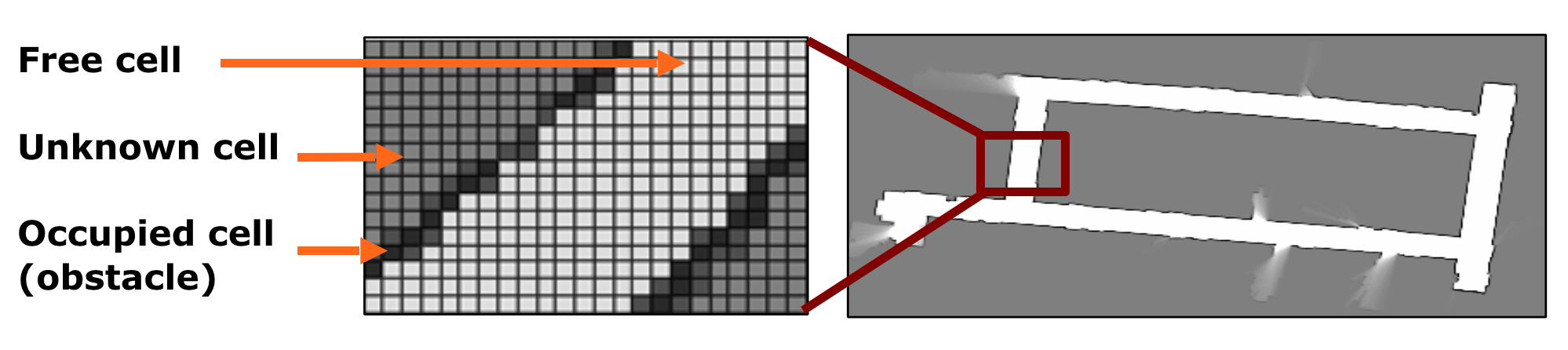
Figure 2. Bayesian grid mapping. Each cell in the map can represent free space (white), obstacles (black), or an unknown state (grey) if it has never been observed.

The goal of map reconstruction is to generate a detailed and accurate map. In terms of map representation, this work uses an occupancy grid, which is widely used for mobile robot navigation (Thrun et al., 2005) and can be easily understood by human users. As shown in Fig. 2, each cell (i.e., grid) on the map can be in one of three states: “free” when it is empty, “occupied” when it contains an obstacle or “unknown” when it has never been observed. With these three states, place reachability can be inferred, allowing safe and fast navigation.

4.1. Challenges: Sparsity and Noise Issues

Before diving into the technical details, we first study the challenges of mmWave based grid mapping. A mmWave radar detects ambient objects based on signal reflection. After several on-board pre-processing steps (e.g., interference mitigation), the range and orientation of reflecting points can be estimated and these points collectively form a point cloud in the field of view. However, unlike the dense point clouds generated by lidars or depth cameras, the mmWave point cloud in indoor environment has two fundamental issues: i) multi-path noise and ii) sparsity.

4.1.1. Multi-path Noise

Similar to any radio frequency technology, the signal propagation of MIMO mmWave in indoor environments is subject to multi-path issue due to aliasing from imperfect beams (Jog et al., 2019) and reflection from surrounding objects (see Fig. 3(a)). As a consequence, reflected signals arriving at a receiver antenna are normally from two or more paths, leading to smearing and jitter. Multi-path is the primary contributor to the non-negligible proportion of pertinent noise artefacts or ‘ghost points’ in a mmWave point cloud. Given $\sim 15$m bound of our indoor environment, we empirically found that, in extremely severe multi-path scenarios, e.g., corridor corners, ghost points can account for $>75\%$ points of a frame, which severely impacts grid mapping steps. Fig. 3(b) shows examples of noisy point clouds, where we can see many ghost points behind walls.

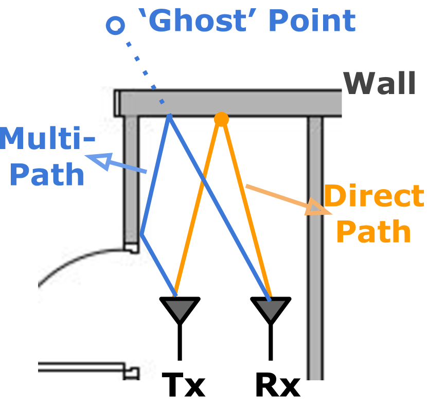
(a) Illustration.

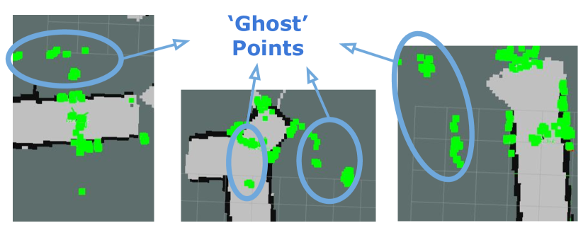
(b) Examples

Figure 3. Multi-path Noise. The black lines in (3(b)) are walls and there are non-negligible noise artefacts (in green) behind walls that are the result of multi-path reflection.

4.1.2. Sparsity

As shown in Fig. 4, the point cloud given by a single-chip mmWave radar is approximately $\sim 100$ reflective points per scan, which is over $100\times$ sparser than a lidar. Such sparsity results from three factors, including (1) the fundamental specularity of mmWave signals, (2) the low-cost single-chip design and (3) restricted sensing range by manually settings. Wireless mmWave signals are highly specular i.e., the signals exhibit mirror-like reflections from objects (Guan et al., 2020). As a result, not all reflections from the object propagate back to the mmWave receiver and major parts of the reflecting objects do not appear in the point cloud. Moreover, unlike massive array radar technology, due to cost and size constraints, the mmWave radar in our use only has $7$ antennas, which fundamentally limits its resolution. Moreover, as opposed to massive MIMO radar technologies, the mmWave radar in this case only has $3\times 4$ antennas. Such a design is effective in both cost and size but results in poor angular resolution ($15^{\circ}$ in azimuth, $58^{\circ}$ in elevation) and targets which are closely spaced will be ‘smeared’ together. Moreover, in order to lower bandwidth and improve signal-to-noise ratio, algorithms such as CFAR (Constant False Alarm Rate) (Ward, 1969) are used for data processing and only provide an aggregated point cloud, further reducing density. The third factor resulting in sparsity is specific to indoor mapping tasks and a consequence of multi-path noise. mmWave point clouds contain a non-negligible portion of ‘ghost points’, which can mislead map densification. In order to suppress these ‘ghost points’, we discard points outside of a sensing radius of $6$m, as multi-path effects generally incur false-positive points at longer distances (Yan et al., 2016). However, this restriction inevitably decreases the density of point clouds further.

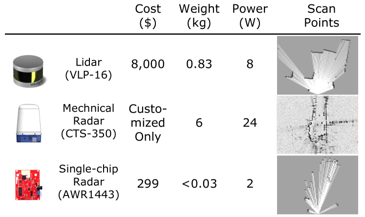
Figure 4. Comparison of lidar, mechanical radar and our single-chip radar. In each category, the features of a representative model are listed. Notably, compared with a lidar and a mechanical radar (Weston et al., 2018), our beamforming radar is much cheaper and lighter, but only provides few points.

4.2. Reconstruction Framework

With knowledge of the properties of mmWave data, milliMap aims to create a dense grid map. Owing to the complex interaction of the aforementioned challenges, this essentially requires an upsampling approach that can simultaneously address the sparsity and noise/outlier issues, which is far from trivial. Such a huge design challenge makes classic methods based on heuristics inadequate here (as seen in Sec. 7.1).

Reconstruction Neural Network. To address the sparsity and noise challenge, we propose to use generative neural network (i.e., GAN in this work) reconstruct maps. As discussed in Sec. 2.2, conditional GAN is a learning paradigm that has proved to be a very effective tool for improving image resolution and generating realistic looking images. More importantly, GAN has the proven ability to reconstruct details (Yang et al., 2018), which can be crucial for route planning for search and rescue. Intuitively, GAN can utilize receptive fields in its CNN generator to denoise and densify image patches by referring to its neighboring contexts. Therefore, the generator in GAN can learn to fill in the missing gaps due to sparsity and eliminates artifacts caused by multipath. The discriminator in GAN further allows us to recover the underlying outline similar to the real ones. In fact, using GAN to perform denoising (Yan and Wang, 2017) and super resolution (Ledig et al., 2017) has become a predominant fashion in the computer vision field when heuristics fall short. Concretely, our adopted network architecture is constructed based on pix2pixHD (Wang et al., 2018), which is a recently proposed encoder-decoder framework based on conditional GAN (Mirza and Osindero, 2014). It comprises of a generator $G$ and a discriminator $D$. In our context, the goal of the generator $G$ is to transform sparse and noisy patches to dense and clean images, while the discriminator $D$ aims to distinguish real images (i.e., partial environment maps) from the transformed ones. As in many other generative networks, U-Net (Ronneberger et al., 2015) is adopted as the backbone in our generator. To allow a large receptive field without large memory overhead, our network also uses multi-scale discriminators and downsamples the real and synthesized images by different factors to create an image pyramid of various scales. The discriminators are trained to distinguish real and generated images at various scales.

Cross-modal Supervision by Collocation: Training the above neural network requires a large number of labelled images. However in reality, actual maps are not always available and even when they are, maps can be outdated because in general most buildings do not precisely match with blueprints (Thrun, 2002). Manually calibrating each map incurs huge labor costs and is hard to scale. On the other hand, it is a common practice to use lidar to map indoor/outdoor environments (Zhang and Singh, 2014; Tomoiagă et al., 2016; KUKA, [n. d.]). Modern lidar can be very accurate and we therefore consider to use it for creating a fresh map that is consistent with the mmWave radar observations. To achieve such a generic and cheap labeling manner, milliMap adopts a cross-modal supervised learning fashion by using only partial labels (i.e., lidar patches) generated from a co-located lidar, allowing a robot to learn about the occupancy of the indoor environment by simply traversing an environment. After the learning phase, the mmWave radar on the robot is able to gain mapping skills from past experience and becomes capable of generating a lidar-like map independently.

4.3. Network Input

Given the above neural network, it is not immediately clear what representation of the inputs is best. Similar to most networks for image-to-image translation, our network expects image-like inputs, with a fixed, relatively low, number of channels and spatial correlations between neighbouring pixels. This is not met by the inherent irregularity of point clouds. We thus need to firstly convert the point cloud to an image-like representation and then use existing networks to process it.

Limitation of Scan Inputs. Perhaps the most straightforward representation is a virtual 2D laser scan obtained from the 3D point cloud. After projecting each scan to a planar 2D image via raytracing, generative convolutional neural networks are able to take it as an input and generate a denser and denoised image. The dense images can then be converted back to angular distance measurements via raytracing and used for mapping. However, as the mmWave point cloud is very sparse, the converted scan image from each frame contains few spatial correlations between neighboring pixels. Directly feeding such non-informative images to a network incurs overfitting and hard to generalize in new environments (Theis et al., 2015). For these reasons as well as our goal for developing 2D maps (i.e., z-axis is not needed for end maps), in this work we chose to work directly on map 2D patches.

Patches as Input The way map patches are generated differs between the training and prediction phases. During training, since we have access to the full, yet sparse, grid maps through running off-the-shelf Bayesian grid mapping (Hornung et al., 2013), we can generate patches by dividing the full map into a regular grid of patches of a given size ($6\times 6m^{2}$ in this work), with an overlap of $50\%$. However, at prediction time, we only generate patches along the robot’s trajectory, in order to reduce inference time. In particular, since we have access to a reasonably accurate odometry (e.g. from wheel odometry and/or inertial measurements), we can detect when the robot is moving out of the current patch, and extract a new patch along the direction of travel, without overlapping with the previous patch ($6\times 6m^{2}$). This simplification ensures we don’t have to merge two overlapping predictions. We then feed patches of the generated map along with the past robot trajectory to our network for denoising and densification. The advantage of this hybrid approach is that patches are built in real-time, whilst the more expensive map densification process is only triggered when entering a new patch. Hereafter, we denote the reconstructed map patches as $\mathbf{x}$ and the noisy mmWave patches as $\mathbf{s}$. The pivotal goal of milliMap is to translate mmWave patches to dense map patches through a deep neural network. The dense patches are then stitched together to produce a full map.

4.4. Reconstruction Loss Functions

The objective function of our network is comprised of losses from four sources: (1) a conditional GAN, (2) an intermediate feature matching, (3) a perceptual loss, and (4) a map prior.

Reconstruction Likelihood. We use conditional GANs to model the conditional distribution of real map patches $\mathbf{x}$ given the input mmWave map patches $\mathbf{s}$, which are converted from the sparse point cloud. The conditional GAN loss can be expressed as:

$$\begin{split}\mathcal{L}_{cGAN}(G,D_{k})=&\mathbb{E}_{(\mathbf{s},\mathbf{x})}[\log D_{k}(\mathbf{s},\mathbf{x})]\\ +&\mathbb{E}_{\mathbf{s}}[\log(1-D_{k}(\mathbf{s},G(\mathbf{s}))]\end{split}$$

where $G$ tries to minimize this objective function against an adversary network $D_{k}$ that tries to maximize it (Mirza and Osindero, 2014). In particular, as our network uses multi-scale discriminators, $D_{k}$ here is the specific discriminator for $k$-th scale. In the meantime, to stabilize training and generate meaningful statistics at multiple scales, we follow (Dosovitskiy and Brox, 2016; Wang et al., 2018) and introduce the feature matching loss $\mathcal{L}_{FM}(G,D_{k})$ in our objective function:

$$\mathcal{L}_{FM}(G,D_{k})=\mathbb{E}_{(\mathbf{s},\mathbf{x})}\sum_{i=1}^{T}\frac{1}{N_{i}}||D^{(i)}_{k}(\mathbf{s},\mathbf{x})-D^{(i)}_{k}(\mathbf{s},G(\mathbf{s}))||_{1}$$

where $T$ is the total number of layers, $D^{(i)}_{k}$ produces the features of $i$-th layer and $N_{i}$ denotes the number of nodes in that layer. milliMap computes this feature matching loss on multiple discriminators which is in line with our multi-scale architecture. Lastly, to compare high level differences and stabilize GAN training (Johnson et al., 2016), we also introduce a perceptual loss in the objective function:

$$\mathcal{L}_{VGG}(G)=\mathbb{E}_{(\mathbf{s},\mathbf{x})}\sum_{j=1}^{J}||F^{(j)}(G(\mathbf{s}))-F^{(j)}(\mathbf{x})||_{1}$$

where $F$ is a pre-trained loss network used for image classification that helps to quantify the perceptual differences of the content between images. In this work, we follow (Johnson et al., 2016) and adopt the VGG network as $F$. Each layer $j$ in the VGG network measures different levels of perception.

Map Prior. The above losses only consider the efficacy of reconstruction in the latent space of high-level appearance but ignore the important low-level geometrics. Recent research found that the latent spaces of appearance and geometry are not strongly correlated. Standard neural network generators can learn appearance transformation, however, lack the ability to embed complex geometry cues for effective image-to-image translation (Gokaslan et al., 2018; Zhu et al., 2017a). Nevertheless, 2D indoor maps in modern buildings often have strong geometric structures that follow certain patterns, e.g. following rectilinear outlines for ease of construction. As this geometric information is fairly ubiquitous (Garulli et al., 2005), one can leverage it as a prior to bootstrap the patch generation process and enhance the quality of the final stitched map. Formally, given a generated patch $G(\mathbf{s})$ and its corresponding real patch $\mathbf{x}$, we define a map-prior loss as follows:

(3) $$\mathcal{L}_{MP}(G)=\mathbb{E}_{(\mathbf{s},\mathbf{x})}\sum_{j=1}^{M}||\mathbf{h}^{(j)}\ast G(\mathbf{s})-\mathbf{h}^{(j)}\ast\mathbf{x}||_{1}$$

where $\ast$ represents the convolution operator and $\mathbf{h}^{(j)}$ is one of $M$ convolution kernels with fixed weights, determined by the types of convolution. For example, $\mathbf{h}^{(j)}$ can be a line or edge detection mask, capturing different geometric properties of images. Through a detector mask, this map-prior loss encourages the consistency between source and target patches corresponding to a certain geometric prior. For example, many objects (e.g., walls and doors) on indoor floor plans are line based (Garulli et al., 2005). Therefore, when using line detectors to embed such a prior in the loss, we can achieve better reconstruction performances in corridors, as shown in Fig. 5. Choices of convolution masks are flexible, mainly depending on the noise level of inputs as well as a particular map/building type. We will quantitatively discuss the impacts of different types of detectors in Sec. 7.2.

Finally, our full objective combines reconstruction likelihood and map prior as:

(4) $$\begin{split}\mathcal{L}_{total}=\sum_{k=1,2,\ldots,K}&\mathcal{L}_{cGAN}(G,D_{k})+\lambda_{1}\mathcal{L}_{FM}(G,D_{k})\\ +&\lambda_{2}\mathcal{L}_{VGG}(G)+\lambda_{3}\mathcal{L}_{MP}(G)\end{split}$$

where $\lambda_{1}$, $\lambda_{2}$ and $\lambda_{3}$ are hyper-parameters for regularization. $K$ denotes the number of distinct scales for discriminators.

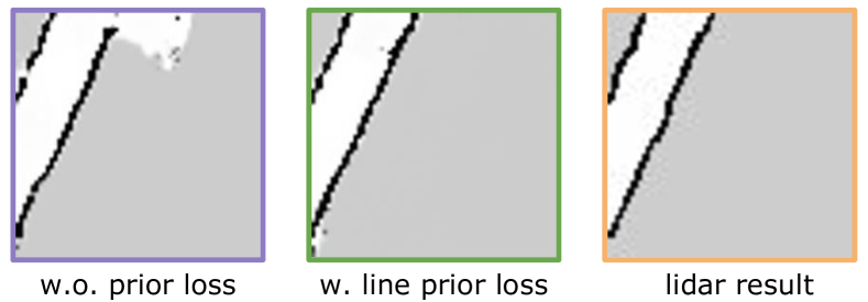
Figure 5. Effectiveness of map prior loss on a straight corridor patch. A line detector is used in this case to construct the map-prior loss and the produced ‘corridor’ is straighter and more complete. lidar is used as pseudo-ground truth.

5. Semantic Mapping

So far we have introduced how milliMap reconstructs a dense grid map from mmWave signals. Nevertheless, in order to best assist the decision making of emergency response, a thorough map should not only tell where the obstacles are but also their semantics. Exhausting the whole universe of indoor semantics is beyond the scope of this work; instead milliMap follows (Tashakkori et al., 2016) and focuses on $4$ predominant construction objects that semantically describe space accessibility: (1) horizontal access object (AO) - doors, (2) vertical AO - lifts, (3) alternative AO - glass and (4) non-AO - walls.

5.1. Complex Construction Objects

Challenge. The main challenge here lies in the complexity of interior construction objects, with prior art on material identification difficult to directly apply. Specifically, previous work focuses on objects made of a single material or containing very thin layers (e.g., cardboard box). For these simple objects, the received mmWave signals are from the specular reflection from the object surface and thus prior work (e.g., (Zhu et al., 2015b)) can directly use the strongest/peak signal strength (RSS) value to determine the object type. However in our case, many construction objects in indoor environments, ranging from composite walls to hollow doors, consist of multiple slabs made from different materials. For instance, fig. 6(a) shows the diagram of common interior building wall, in which $5$ different layers are stacked together. Each of the slabs often has sufficient thickness that affects propagation characteristics of mmWave signals as well as resulting in multiple reflections from internal layers (Holloway et al., 1997). Additionally as discussed in (Kuga and Phu, 1996; Goulianos et al., 2017), building materials have different roughness and the diffusion effect of mmWave on some rough surfaces (e.g., the surface of wall) can be significant. Such diffusion effects, unfortunately, further complicates the problem of object identification (see Fig. 6(b)). Intuitively, the compound effect of diffusion, multiple internal reflections and specular reflection is hard to model by only using a peak RSS value.

Key Idea and Observations. From the perspective of a receiver, both diffusion and multiple internal reflections cause multi-path effects. Owing to differences in several properties, such as roughness and interior layers, the multi-path effects exhibit certain patterns, captured in the 1D range FFT profile (see Sec. 2.1 for definition). Fig. 7(a) shows an example of a range FFT profile. The peak value in this example represents the normalized intensity of the specular reflection along the direct path, where neighbor values around it are due to multi-path effects from diffusion and multi-reflections. To illustrate what patterns we can extract from the shape of the peak, we extract features (e.g. peak value, standard deviation) from $27,952$ collected profiles of $3$ common construction objects. Fig. 7(b), 7(d) and 7(c) show the average value and standard deviations, from which two key observations can be drawn. First, peak value differences (feature index $2$) between construction objects can be vague (e.g., glass versus lift) that confuses object classification. Second, both the magnitude and shape of neighboring points exhibit more distinct patterns, providing better object signatures.

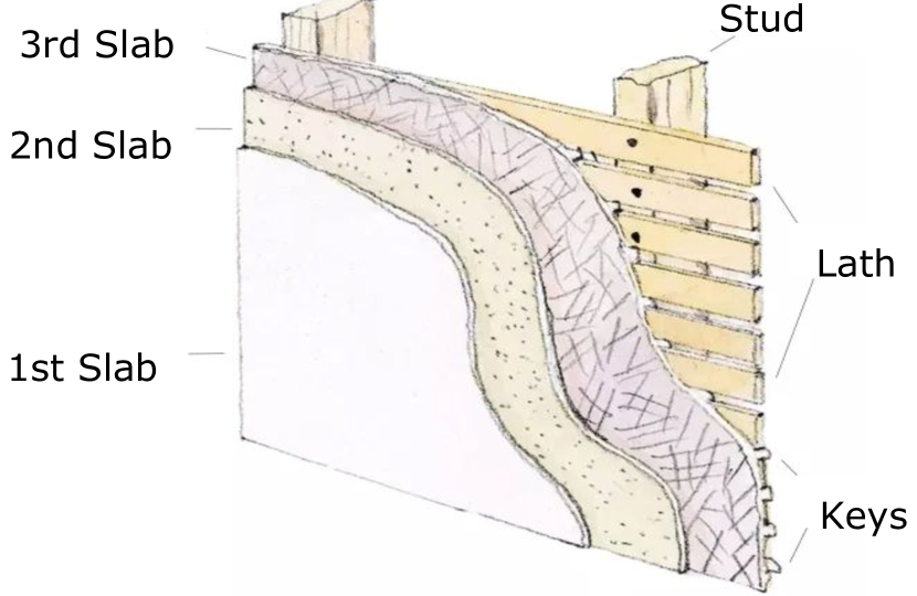
(a)

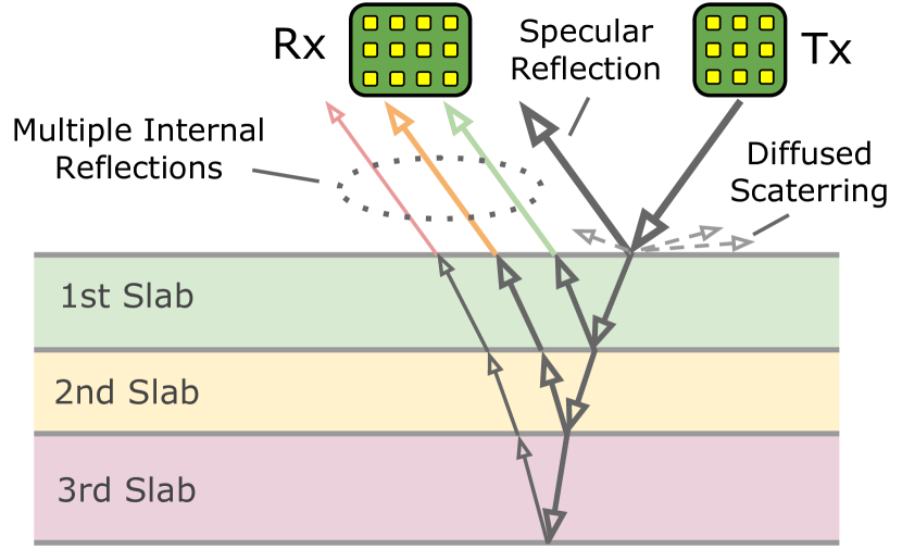
(b)

Figure 6. mmWave signal propagation on a wall. (6(a)) A common interior building wall has multiple layers. (6(b)) The diffusion and multiple internal reflections on a simplified wall model (with only three slabs), result in complicated multi-path effects. We exploit these signatures for classification.

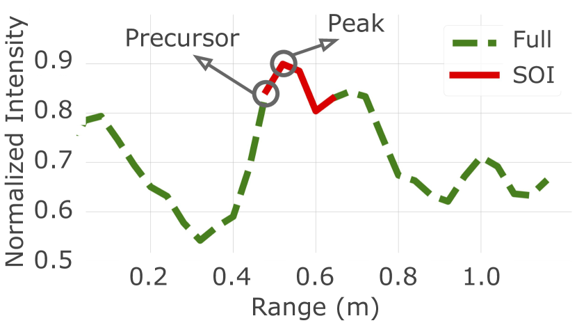
(a) SOI Extraction

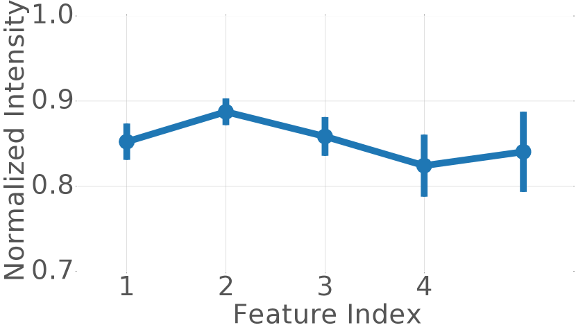
(b) Door

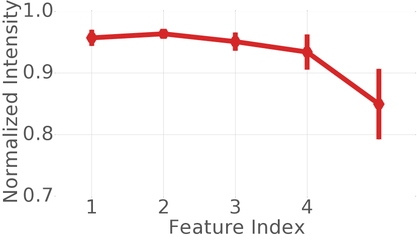
(c) Lift

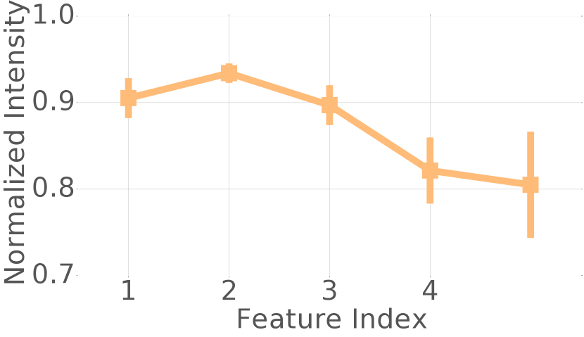
(d) Glass

Figure 7. Semantic Mapping: (a) $16$cm-wide SOI, determined by the corresponding peak in the range FFT profile; (b-d) ‘average’ SOI aggregated from $27,952$ training samples. SOIs of different materials have distinct patterns. Note that the first feature index, namely the starting point in (b-d) is the precursor index to the detected peak value.

5.2. Semantic Recognizer

Based on the above observations, we propose a semantic recognizer that operates by first extracting a segment of interest from the range FFT profile, and then using a classifier to identify different types of obstacles.

Segment of Interest. Notably, the first step before performing segment extraction is to acquire a scan at a perpendicular angle to the object. To combat the limited angular resolution of the TI board (see Sec. 2, milliMap tasks the robot platform to mechanically scan its horizontal field of view, and then determines the perpendicular angle by pinpointing the pose that yields the largest reflection intensity. Once a perpendicular pose is determined, the robot platform enters the static mode and starts to record the range profile at this instant. A practical issue of applying the above intuition is determining the number of points to consider after the peak, namely finding a segment of interest (SOI) in the range profile. As multiple objects are in the mmWave radar’s field of view, a range profile often contains extraneous information corresponding to non-target objects. Directly using the whole profile as features will thus confuse a single object classifier. As the target object in our case is the nearest object perpendicular to the robot/radar, the starting point of a SOI is easy to find because it has the steepest increasing gradient in the profile. To mitigate the potential aliasing issue due to $40$mm ranging resolution, we always use the prior index to the steepest point as the starting point of SOI. We empirically found that at a SOI width of $6$ points, the best tradeoff can be achieved. In Sec. 7.6, we will further discuss the impact of different SOI widths on semantic classification. Fig. 7(a) illustrates the SOI extraction process.

Object Classifier. Taking the extracted SOI as input, a classifier is used to identify a target object. The classifier adopted by milliMap is a convolution neural network (CNN), which is widely used in many classification tasks for its superior accuracy and efficiency. Specifically, this classifier comprises of three 1D convolution layers and a dense layer with softmax activation. The kernel sizes and strides of all three convolution layers $32$ and $1$, and the activation functions are Exponential Linear Unit (ELU). We compare the performance of this CNN classifier with other baseline classifiers in Sec. 7.1 to further justify our choice.

6. Implementation

For the purpose of reproducing our approach, we release our dataset and the source code at https://github.com/ChristopherLu/milliMap.

Multi-modal Robotic Sensing Platform. A Turtlebot 2 platform equipped with multiple sensors is used a a prototype data collection platform. This dataset contains synchronized mmWave point cloud data from a TI AWR1443 board, lidar data from a Velodyne VLP-16 and wheel odometry. The bandwidth of the used radar is $4$GHz (77GHz - 81GHz) which yields a ranging resolution of $\sim 4$cm. It has $120$ degree azimuth field of view and $30$ degree elevation field of view. In addition, we provide RGB images from a front-facing monocular camera. The mmWave sensor, lidar and camera are coaxially located on the robot along the vertical axis. The navigation of the mobile robot is implemented using ROS (Quigley et al., 2009) on a Linux notebook, which is a widely adopted practice in the robotics community. Besides controlling, the notebook is also responsible for sensor data storage. Once the collection phase is completed, the notebook sends the collection back to a backend server for offline model training. During the online phase, model inference is expected to be done either by an embedded GPU or the notebook itself. We will discuss the real-time performance soon in Sec. 7.7.

Testbeds. Two buildings are surveyed at the time of writing. The A Building has a size of $\sim 1,100m^{2}$ and contains four floors, mostly composed of corridors and atrium; the B Building has a size of $\sim 205m^{2}$ and contains one floor with a combination of corridors and rooms. The A Building dataset presents a combination of walls, doors, lifts and large glass handrails; the B Building dataset presents walls, doors, glass panes, lifts and clutter. Notably, despite similar high-level semantics, these buildings differ in pathway widths, door types, glass sizes and more importantly, layouts.

Data Collection Procedure. To collect the dataset of map reconstruction, we use a remote control to drive our mobile robot moving from a starting point to an end point on each floor of the buildings. Particularly, we do not set any specific traveling routes in data collection, but let the robot freely traverse the indoor space. The reconstruction dataset contains the data from the mmWave radar, lidar and wheel odometry. Sec. 7.1 introduces how the collected data are used for training and testing. The semantic mapping dataset is acquired in the same places as above. In data collection, a mmWave radar on the robot is firstly rotated to a pose perpendicular to the target object/material surface with a distance $\sim 0.5$ meter. Then at each collection point, we acquire data at a rate of $10$Hz and semantically label these offline from location logs. In total, we collected $45,535$ frames from $4$ types of objects in two buildings.

7. Experimental evaluation

7.1. Grid Map Reconstruction Performance

We start with the validation of the grid map reconstruction method proposed in Sec. 4.

Evaluation Metrics. Throughout this section, two metrics are consistently adopted to quantify map reconstruction performances: mean absolute error ($L_{1}$) and mean intersection-over-union (IoU), both of which are widely used (Weston et al., 2018). The mean $L_{1}$ is calculated as follows (Zhao et al., 2016):

(5) $$L_{1}=\frac{1}{N}\sum_{p\in P}|x(p)-y(p)|$$

where $p$ is the index of the pixel and $P$ is the patch. $x(p)$ and $y(p)$ are the values of the pixels in the processed patch and the ground truth respectively. We will omit “mean” hereafter for presentation ease. It is worth mentioning that as the image resolution is $1$dm/pixel in our case, the $L_{1}$ mapping error is thus in the units of decimeters. It is also worth mentioning that our goal is to build an indoor map for navigation in search and rescue applications. Therefore it is necessary to have a good idea of the free space and obstacles. Although this property is difficult to be numerically reported, we will qualitatively discuss it when comparing reconstruction results.

Evaluation Protocol. We perform cross-floor and cross-building tests to examine the effectiveness of the trained model. To avoid the known overfitting issues of DNN in our model and we particularly follow this cross-test evaluation principle on unseen scenarios. Concretely, our collected dataset is divided into training and testing sets. In particular, the training set contains $12,000$ augmented patch images extracted from maps of the 1st, 2nd and 3rd floors in A Building. The data augmentation strategy we adopt here is the standard rotation and translation transformations on original patches to promote model generalization. Our test set comprises $49$ patch images extracted from maps of the 4th floor in A Building and $12$ patches extracted from the 2nd floor of B Building.As introduced in Sec. 6, the environments of A Building and B Building notably differ in pathway widths, door types, glass sizes and more importantly, layouts etc.Moreover, the path followed by our robot on the 4th floor is quite different from that of other three floors in A Building. The above scenario variety helps us maximally follow the cross-testing principle.

All training and testing patch images have size $64\times 64$. Concerning model training, three loss weights $\lambda_{1}$, $\lambda_{2}$ and $\lambda_{3}$ are set to $10$, $10$ and $5$ respectively. We adopt a line detector as the convolution kernel in Eq. (3), $M$ is set to $4$, corresponding to $4$ line directions in $0\mathrm{°}$, $45\mathrm{°}$, $90\mathrm{°}$ and $135\mathrm{°}$. The training batch size is set to $16$ and we use the Adam optimizer at a learning rate of $2e^{-3}$.

Table 1. Densification Before and After Mapping.

	Method	A Building		B Building
		L1	IoU	L1	IoU
Scan (before)	Pix2Pix (Isola et al., 2017)	2.776	0.186	3.602	0.150
	Pix2PixHD (Wang et al., 2018)	2.309	0.226	3.722	0.152
Patch (after)	Pix2Pix (Isola et al., 2017)	2.214	0.319	3.200	0.173
	Pix2PixHD (Wang et al., 2018)	2.096	0.380	2.752	0.239

Effectiveness of Densification Before and After Mapping. We first investigate the effect of two input representations (refer to Section 4.3): (i) we perform densification of each scan and then aggregate them using grid mapping (denoted as scan representation) and (ii) we aggregate scans using grid mapping and then perform densification on image patches (denoted as patch representation). As Tab. 1 shows, the reconstruction results of patch representation are significantly better than scan for both networks, implying the effectiveness of patch representation. Given the best-performing Pix2PixHD network, the $L_{1}$ errors of scan are $20\%$ inferior to patch, with over $35\%$ inferior IoU scores on both datasets. The reason is that the single scan densification easily overfits to straight lines, which is consistent with our discussion in Sec. 4.3.

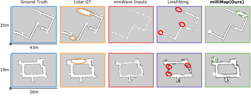
Figure 8. Qualitative reconstruction results. milliMap achieves a comparable performance to the lidar counterpart. Solid circles on Lidar GT are glass objects; dashed circles are ‘ghost areas’ in generation. Red circles show corridors that have been erroneously closed by the line-fitting method (false obstacles). Top Row: A Building; Bottom Row: B Building.

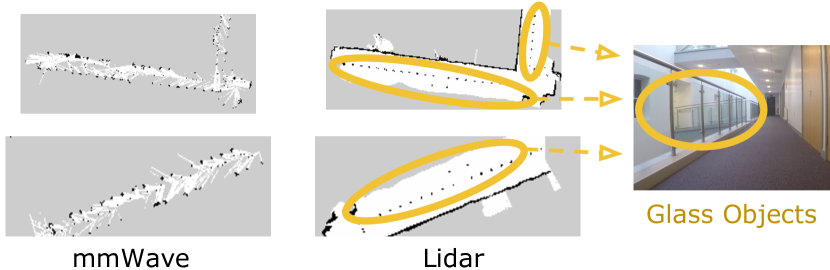
Figure 9. Incorrect lidar supervision due to presence of glass objects in training data.

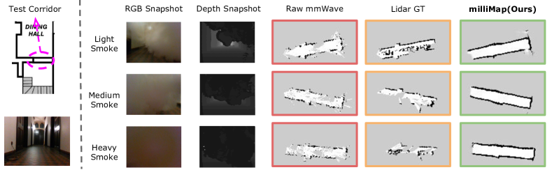
Figure 10. Qualitative testing in smoke-filled environments.

Network Architecture Validation After understanding the effective processing order, we adopt the patch representation for subsequent experiments and continue to validate different architectures of reconstruction networks. As milliMap is the first indoor mapping work dealing with very sparse inputs of such low-cost mmWave radar, we can only compare the following commonly used generative networks: Conditional Variational Autoencoder (CVAE) (Weston et al., 2018), BicycleGAN (Zhu et al., 2017c), Pix2Pix (Isola et al., 2017) and Pix2PixHD (Wang et al., 2018). Notably, CVAE is the network architecture adopted by (Weston et al., 2018), though their goal is not sparse-to-dense due to the use of a customized mechanical radar. Beside these deep learning methods, we also compare with lineFitting (Pfister et al., 2003), a classic reconstruction method for line-based indoor floor plans. Tab. 2 shows the performance comparison of different reconstruction methods. Despite its success on lidar map reconstruction, the classic line fitting method obviously struggles on both datasets and provides $<50\%$ IoU than our approach, attributed to the substantial sparsity in raw mmWave maps. In particular, it is observed in Fig. 8 that there are many falsely closed corridors predicted by the line fitting method. Such misclassified free space and navigable routes is contrary to our goal for safe/efficient navigation as areas falsely marked as obstacles are in general more detrimental than areas falsely marked as free space, since a robot or a firefighter is typically capable of avoiding unpredicted obstacles. In contrast, when computing a path to a certain location, falsely closed corridors could make whole areas of the building appear inaccessible. On the side of DNN methods, we did not find the advantages of using variational methods, implying that random sampling from a learnt distribution actually counteracts the benefits of uncertainty modelling and tends to output blurred reconstructions. We hypothesize that the performance gain can be also attributed to the strong regularity within indoor maps, which favors deterministic learning methods. Lastly, despite their close correlation, we found that Pix2PixHD outperforms Pix2Pix on both datasets, thanks to the use of multi-scale discriminators and more losses. By introducing the map-prior loss, our method can further gain $9.6\%$ L1 accuracy than Pix2PixHD, and $\sim 5\%$ better IoU performance overall on both datasets, which is a comparable delta to the field of image reconstruction/translation (Zhu et al., 2017a). Note that the prior loss is simply an additional loss term that incurs no further computation overhead for either inference or training; however, it still leads to a performance increase.

Explanation of ‘Ghost’ Areas. Interestingly, in the last column of Fig. 8, there are ‘ghost’ areas on the generated maps, where part of a wall (black) is incorrectly marked as free regions (white). Recall that we adopt a cross-modal supervised learning framework that uses lidar patches as supervision labels. These labels, however, can be error-prone when encountering glass objects (see the second column in Fig. 8), which is a commonly-known limitation of lidar. Although glass is opaque to mmWave, considering the high appearance similarity (see Fig. 9), we hypothesize the ‘ghost area’ of our generated grid map of A Building can be attributed to the misleading lidar patches of glass in training. ‘Ghost’ areas do not appear with scan inputs, due to its overfitting to straight corridors.

Table 2. Reconstruction method comparison.

Method	A Building		B Building
	L1	IoU	L1	IoU
LineFitting (Pfister et al., 2003)	3.180	0.167	4.114	0.103
CVAE (Weston et al., 2018)	2.408	0.323	3.082	0.221
BicycleGAN (Zhu et al., 2017c)	2.538	0.303	3.393	0.195
Pix2Pix (Isola et al., 2017)	2.214	0.319	3.200	0.173
Pix2PixHD (Wang et al., 2018)	2.096	0.380	2.752	0.239
Ours	1.976	0.402	2.536	0.247

7.2. Effectiveness of Sub-components

In order to understand the contribution of key sub-components in the reconstruction neural network, we further conduct an effectiveness analysis on: i) loss functions and ii) multi-scale discriminators.

Different Loss Functions. We modify the objective function of Eq. 4, by alternating different loss terms for reconstruction likelihood as well as alternating variants of our proposed map-prior term. Tab. 3 shows that feature matching loss plays a vital role which brings $16\%-24\%$ gain in $L_{1}$. The perceptual loss (i.e., VGG loss) also helps and removing it incurs a average performance decline ($\sim 7\%$) on both datasets. This is reasonable because the VGG network is pre-trained by general image classification tasks and hence becomes less effective in our specific mapping task.

These experiments indicate that, although grid maps are more about geometrics, these appearance losses are still important for stabilising generator training and improving realism. Interestingly, when we implement the map prior loss as edge detectors, its efficacy is not as helpful as the line detectors. This is because edges are a broad concept for any image and cannot effectively incorporate the geometrics of line-based maps. Moreover, as our supervision signals are from the imperfect lidar patches, the edge detectors are sensitive to the noises of lidar. In contrast, line detectors focus on low-frequency components of images and thus can be more robust to noise.

Number of Scales. Next we examine the impact of multi-scale discriminators. Recall that milliMap uses a $2$-scale discriminator while our ablation study further examines the cases of $1$- and $3$-scales. As shown in Tab. 3, the overall impact of multi-scale discriminators is not substantial ($\sim 5\%$) when varying the number of scales. This is as expected because the multi-scale discriminators were originally designed for high-resolution images while our input patches are not. We observed a marginal improvement from single-scale to $2$-scale discriminators as more diverse feature matching is introduced in different scales. However, such increase of scales soon counteracts the benefits when the $3$-scale network becomes oversized and overfits. This overfitting issue is more obvious on B Building dataset due to cross-building testing.

7.3. Testing in Smoke-filled Environments

Thick smoke is a common event that occurs in many emergency incidents such as firefighting. In this experiment we examine the potential use of milliMap in smoke-filled environments. To this end, we use a smoke machine to create different smoke densities in a corridor ($12\times 1.5$m²) in another building where various sensor data were collected on the robotic platform for comparison, including lidar, depth camera, RGB-camera and mmWave radar. Fig. 10 shows the reconstructed map in $3$ scenarios with different levels of smoke distributions. As we can see, lidar gives very inaccurate map results even with low levels of smoke. Due to the occlusion and reflection effects of smoke particles, lidar generates many non-existent objects and/or misses a lot of real ones. In fact, even under the lightest smoke condition, lidar already undergoes substantial performance degradation. Depth and RGB cameras also fails to see through smoke due to similar reasons. In contrast, the mmWave radar is able to see through smoke and milliMap reconstructs the corridor accurately in all $3$ smoke-filled scenarios. These results demonstrate that our mmWave based reconstruction model trained in benign environments can transfer its mapping ability to unseen smoke-filled environments. Based on this trial, we believe there are many promising use cases of it for emergency situations.

Table 3. Effectiveness on losses and number of scales.

		A Building		B Building
		L1	IoU	L1	IoU
Losses	w.o. FM	2.408	0.323	3.082	0.221
	w.o. VGG	2.115	0.379	2.762	0.242
	Edge Loss	2.214	0.319	3.200	0.173
# of Scales	1	2.024	0.394	2.633	0.250
	3	2.022	0.387	2.863	0.219
Ours		1.931	0.398	2.589	0.238

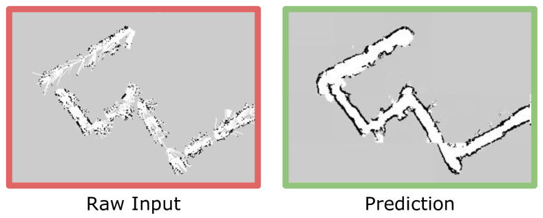
Figure 11. Qualitative result for hand-held cases.

7.4. Extending to Hand-held Devices

First responders, who carry hand-held or helmet-mounted devices, need to work in a team with robots for complementary operations. To this extent, we test milliMap’s potential for map construction on hand-held devices, without retraining, but directly using the model trained using a robot. The main differences are that the odometry of the hand-held device is inferred from an embedded inertial measurement unit by pedestrian dead reckoning (PDR) methods (Jimenez et al., 2009). However, compared to wheel odometry, PDR odometry drifts more and has a lower sampling rate due to step discretization. As a consequence, the raw patch images of PDR are of lower fidelity. Furthermore, due to different viewpoints (e.g., different heights of robots and pedestrians), the mmWave observations have obvious differences from the training samples. Despite these compromising factors, as can be seen in Fig. 11, milliMap still gives a good reconstruction with $\sim 0.83m$ error, providing a much better sense of space accessibility than using raw data alone. This experiment serves to demonstrate how teams of robots and people could build a common map.

7.5. Downstream Navigation Tasks

We now test whether the produced maps, despite their imperfections, can still be used for autonomous navigation. In particular, we investigate if another robot or person is able to localize in the predicted map with comparable accuracy to that of a lidar map. We run Monte Carlo localization using mmWave raw measurements on the reconstructed maps using the standard amcl ROS package with default parameters. Each time the robot or person starts at a random location and samples a radar frame. The pseudo-ground truth is derived by localization with lidar on a lidar map of the same floor. Fig. 12 shows the cumulative error distribution for $50$ Monte Carlo runs. For the reconstructed map of A Building, our robot achieved a mean translation accuracy of $0.285$m and orientation accuracy of $0.142$ rad; on the reconstructed map of B Building, the mean translation and orientation accuracy are $0.178$m and $0.140$ rad respectively. Given the size of the two buildings, these results show that the map produced by milliMap can be used to accurately localize and navigate firefighters or robots.

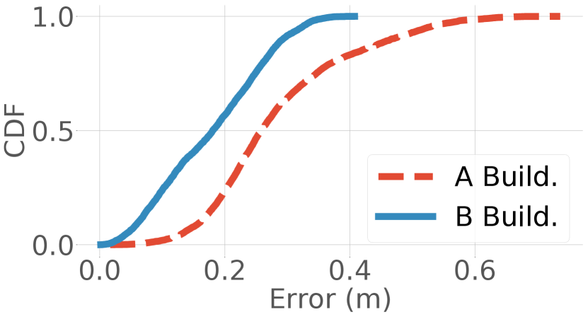
(a) Translation

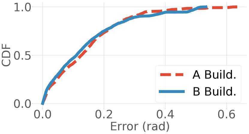
(b) Orientation

Figure 12. Error CDFs for the downstream localization tasks.

7.6. Semantic Mapping Performance

Metrics and Baselines. To validate the performance of semantic classification, we adopt the $4$ metrics for standard classification tasks: accuracy, precision, recall and F1 score. For comparison, we implement RSA (Zhu et al., 2015b), a method identifying objects based on the mmWave reflectivity on different surface materials. Furthermore, to justify our choice of CNN classifier, we also compare with other $4$ commonly used classifiers, including support vector machine (SVM), random forest (RF), k-nearest neighbors (KNN), multi-layer perceptron (MLP). All of these classifiers take as inputs SOI and predict an object label out of glass, lift, wall and door.

Evaluation Protocol. The evaluation protocol here is similar to the one described in Sec. 7.1. Specifically, classifiers are developed on a training set collected from three floors in A Building and we test the trained classifier on a new floor in A Building as well as in a new building of B. Overall, our training and test sets contain $27,952$ and $17,583$ samples (two test buildings) respectively. When training baselines and our classifier, the best model for online inference is determined by 5-fold cross validation.

Overall Performance. Tab. 4 summarizes the semantic mapping performance where a SOI with a width of $6$ is used. Clearly, our CNN classifier achieves the best performance overall on two datasets and MLP classifier is second to it. All shallow-learning based classifiers (i.e., SVM, RF, KNN) underperformed relative to the deep-learning based methods. This is reasonable as MLP and CNN are able to learn meaningful feature representation in training, rather than a shallow classifier on raw data. Because of these meaningful features, MLP and CNN based classifiers can generalize across floors and buildings. In contrast, as RSA only considers the specular reflection from the surface material while ignoring the rich information conveyed by multi-path reflections, it struggles to robustly identify objects in both cases. As expected, cross-building classification (B Building Dataset) is more challenging than cross-floor classification (A Building Dataset) because building differences are more substantial than floor differences, resulting in a performance gap $\sim 15\%$ on average. Fig. 13 further plots the confusion matrix of our CNN classifier. We observed that walls are the most difficult objects to identify on both datasets, coinciding with its greater structural complexity than other objects. In contrast, lifts are generally made of steel, allowing them to be easily identified and yields very high accuracy.

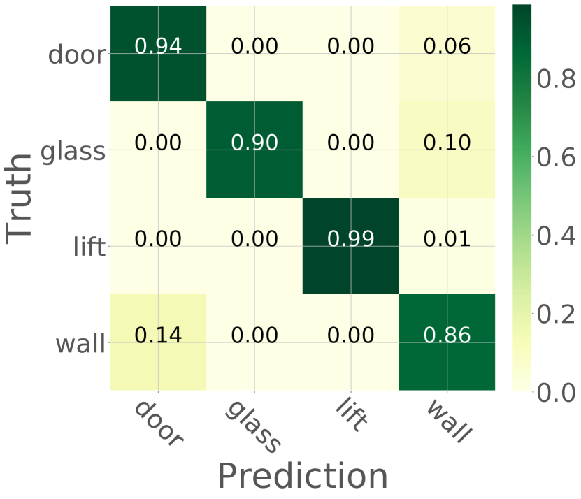
(a) A Building

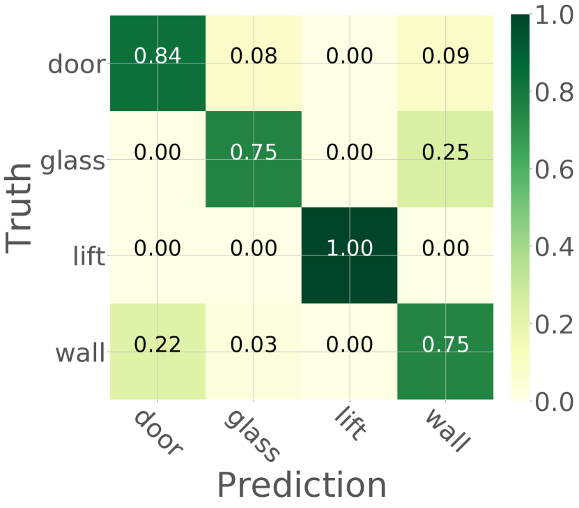
(b) B Building

Figure 13. Confusion Matrix of CNN classifier: (a) A Building (b) B Building.

Table 4. Results of Material Classification: Accuracy (Acc.), Precision (Prec.), Recall (Rec.) and F1 Score.

	A Building				B Building
	Acc.	Prec.	Rec.	F1	Acc.	Prec.	Rec.	F1
RSA	0.67	0.74	0.69	0.71	0.50	0.58	0.53	0.56
KNN	0.83	0.87	0.86	0.87	0.67	0.68	0.75	0.71
SVM	0.82	0.86	0.85	0.85	0.67	0.70	0.68	0.69
RF	0.86	0.89	0.89	0.89	0.67	0.68	0.72	0.70
MLP	0.90	0.92	0.91	0.91	0.74	0.77	0.78	0.77
Ours	0.92	0.93	0.89	0.91	0.80	0.84	0.92	0.88

Impact of SOI Length. The width of SOIs is an important parameter which essentially determines the tradeoff between information richness of features and noise levels. To investigate its impact on the end-to-end object classification, we vary the width from $1$ to $9$, at a step of $1$. As we can see in Fig. 14, an effective width falls into the range of $[4,6]$ while either an over-long or over-short SOI results in a sub-optimal classification result. Notably, the negative impact of over-long SOIs is not as significant as the over-short case for unseen floors (see Fig. 14(a)). We hypothesize that this is attributed to the adopted CNN which likely learns to suppress extraneous information of non-target reflections and such extraneous noise is similar across floors in the same building. However, the limitation of over-long SOIs becomes significant in the case of an unseen building, as suggested by the drop of F1 score in Fig. 14(b). This is reasonable because more different secondary reflections are experienced due to the distinct building structures which makes the learned suppression hard to generalize. Empirically, SOIs with the width of $6$ gives the best overall performance.

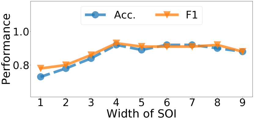
(a) A Building

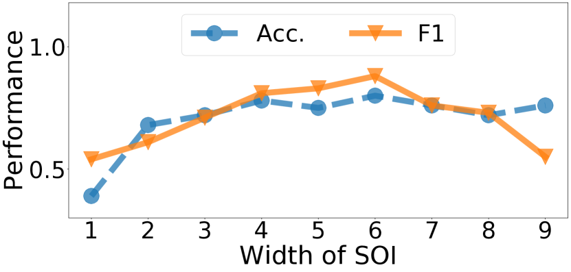
(b) B Building

Figure 14. Impact of the SOI width on semantic mapping.

Dealing with Out-of-set Objects. In real-world applications, it is possible that some objects or materials are not included in the training database, known as out-of-set or foreign/alien objects, and could cause false detections. To detect and mitigate their impacts on our semantic mapping, we introduce an ‘unknown’ label to mark these out-of-set classes. Inspired by the ‘alien device’ detection technique in (Li et al., 2018a), we take the maximum probability value from the class distributions of softmax output (see Sec. 5.2) as a classification score. To distinguish an unknown object from the known ones, we apply a threshold on the classification score - if the score is less than the threshold, we mark the object as unknown. The rationale behind such a score threshold is based on the principles of network learning and that the summation of a softmax distribution is always equal to $1$. Indeed, the goal of learning a CNN classifier is to maximize the softmax probability for individual true classes while a flat probability distribution over multiple classes in testing time often implies an out-of-set label.

As shown in Fig. 15, compared to the samples with the known labels, the probability distribution output by the softmax layer for three out-of-set objects are substantially more scattered and flat. Their resulting classification score is accordingly lower than the known samples. Based on $500$ samples from $5$ different alien objects (e.g., basins, tables, chairs, sofa and fridges.), we empirically found that a threshold of $0.92$ on the softmax classification score can correctly detect over $96\%$ of samples as unknowns. In the meantime, it only results in less than $2.2\%$ false negative rate for known samples.

(a) Various known (in-database) classes.

(b) Out of set: tables

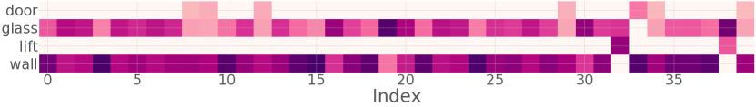
(c) Out of set: chairs

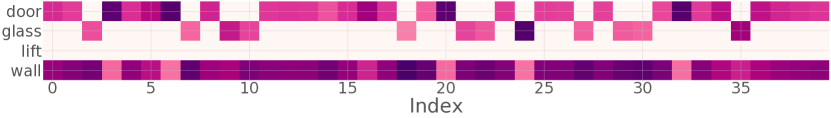
(d) Out of set: basins

Figure 15. Softmax distribution comparison between known classes and out-of-set classes. A dark color represents a large value i.e. high confidence and the horizontal axis denotes sample index. For known labels (top row), the distribution is unimodal. In contrast, the distribution of out-of-set samples are spread over multiple classes, yielding low classification scores.

7.7. System Efficiency

In the last experiment, we investigate the runtime latency, summarized in Tab. 5. Four platforms fitting the payload of mobile robots are used in our evaluation, including Raspberry Pi 3 (RPi 3), Raspberry Pi 4 (RPi 4), NVIDIA Jetson TX2 (TX2) and a mini netbook. In the implementations, we use TensorFlow Lite (Alsing, 2018) to compress our models as per the convention of efficient on-device inference of DNNs. Tab. 5 suggests that both map reconstruction and semantic mapping modules are able to run in real-time on all platforms. Even for the most challenging case (i.e., map reconstruction on RPi 3), a runtime of $2.58$s is also acceptable, because an input patch to our reconstruction network is generated by a robot crossing over a $6\times 6m^{2}$ square (see Sec. 4.3) while most ground robots’ max speeds are $\leq$ 1m/s.

8. Related work

RF-based Imaging and Tracking. Signal reflection of RF waves has been widely leveraged to perform imaging and target tracking. In the WiFi bands, researchers have used commodity WiFi chips (Depatla et al., 2015; Huang et al., 2014; Pu et al., 2013; Liu et al., 2012; Sun et al., 2015; Jiang et al., 2013) to imagine static objects, localize humans and recognize predefined hand gestures. Additionally, by leveraging a specialized FMCW radar (Adib and Katabi, 2013; Adib et al., 2015a, b, 2014; Zhao et al., 2018b; Zhao et al., 2018a, 2019), WiFi signals can be used to accurately track/imagine human body dynamics, as well as recover pose estimation under NLOS scenarios. In the vein of mmWave-based tracking, Babak et al. use FMCW hardware and apply SAR with sparse measurements in absence of device movement noises (Mamandipoor et al., 2014), while Xu et al. uses customized mmWave probe to recover human speeches via throat localization (Xu et al., 2019). On the side of environment sensing, research effort has been devoted to pinpoint indoor major reflectors, thereby combating the environment sensitivity of mmWave communications (Palacios et al., 2017; Wei et al., 2017; Zhou et al., 2019). Nevertheless, major reflectors are still sparse points which are incomparable to the dense grid maps to first responders. Recent works (Zhu et al., 2015a, 2017b) pioneered the research of low-cost mmWave devices to explicitly image objects. By continuously moving or navigating in front of a specific object, they can infer the geometry of small indoor objects. However, such iterative mapping and navigation strategy violates limited time budgetsin search and rescue scenarios. In contrast, milliMap uses a low-cost off-the-shelf mmWave radar to reconstruct a dense occupancy grid map while a robot travels freely in an environment.

RF-based Material/Object Identification. By charactering the reflection intensity of RF signals, the RSA system (Zhu et al., 2015b) measures the reflected mmWave signals at multiple locations and then use an aggregated value to identify a target’s surface material. A similar work is RadarCat (Yeo et al., 2016), a contact based material identification systems leveraging 60 GHz signals. milliMap differs from the RSA and Radar in that it does not require multiple measurements at different locations nor a physical contact with the target material. Recent studies also found mmWave signals can detect and classify hidden electronic devices (Li et al., 2018b) and even screen activities (Li et al., 2020). On the other side, WiFi CSI (Feng et al., 2019), UWB (Dhekne et al., 2018) and RFID (Wang et al., 2017) have recently been utilized to identify materials based on their phase and RSS readings. However, these systems are sensitive to the calibrated positions of pairs of transmitters and receivers, while milliMap is a single-chip solution to mobile robotic platform.

Indoor Mapping/Imaging with non-RF Sensors. Optical sensors, such as RGB cameras (Gao et al., 2014; Dong et al., 2015), laser rangers (Surmann et al., 2003) and stereo cameras (Henry et al., 2014) are established sensor modalities to produce accurate indoor maps. However, these sensors are notoriously fragile under adverse vision conditions, e.g., darkness, glare and smoke debris. Acoustic sensors such as microphones (Mao et al., 2018; Pradhan et al., 2018; Zhou et al., 2017) are recently found to be effective for indoor mapping and object imaging but their performances are restricted by limited sensing ranges and sensitive to environmental noises as well as sound-absorbing materials.

Table 5. Runtime efficiency of key modules in milliMap.

	RPi 3	RPi 4	TX2	Netbook
Map Recon. (s)	2.58	1.01	0.65	0.33
Semantic Mapping (ms)	0.17	0.08	0.06	0.02

9. Limitations and Future Work

This work focuses on a proof-of-principle mapping using mmWave radar, towards our vision of augmenting emergency response with low-cost mobile sensing systems. There are limitations and a number of avenues for future exploration. Firstly, the turtlebot platform is not rugged enough for a real disaster situation. Other more robust platforms have been designed to tackle this problem (Delmerico et al., 2019), e.g. the use of tracked or snake-like robots. Aerial micro-robots are also a potential alternative for rapid exploration, and the form-factor of the single chip radar is ideally suited as a primary sensor for these agents. Secondly, further trials need to be performed under diverse conditions such as different buildings, varying obscurants (e.g. dust in a factory) and under real emergency conditions. Thirdly, we have focussed on using a single agent to build a map, in future work we will explore how to use swarms of robots to cooperatively explore and build the map e.g. by using SLAM (Achtelik et al., 2012).

10. Conclusions

Indoor mapping in low-visibility environments full of airborne particulates is a challenging yet important problem. Particularly of importance to emergency responders, an accurate map can significantly aid in situational awareness and become a life saver in search and rescue scenarios. To this end, milliMap used a mmWave radar on a mobile robot to create a dense map that indicates place reachability and object semantics on the map. We also demonstrated how another agent could relocalize within the map. With extensive experiments in different indoor environments and under smoke-filled conditions, we show the performance of reconstruction, semantic classification and system efficiency of milliMap, demonstrating its ability to generalise to previously unseen environments.

- (1)
- Achtelik et al. (2012) Markus Achtelik, Michael Achtelik, Yorick Brunet, Margarita Chli, Savvas Chatzichristofis, Jean-Dominique Decotignie, Klaus-Michael Doth, Friedrich Fraundorfer, Laurent Kneip, Daniel Gurdan, et al. 2012. Sfly: Swarm of micro flying robots. In 2012 IEEE/RSJ International Conference on Intelligent Robots and Systems. IEEE, 2649–2650.
- Adib et al. (2015a) Fadel Adib, Chen-Yu Hsu, Hongzi Mao, Dina Katabi, and Frédo Durand. 2015a. Capturing the human figure through a wall. ACM Transactions on Graphics 34, 6 (2015), 219.
- Adib et al. (2015b) Fadel Adib, Zachary Kabelac, and Dina Katabi. 2015b. Multi-Person Localization via RF Body Reflections. In NSDI.
- Adib et al. (2014) Fadel Adib, Zach Kabelac, Dina Katabi, and Robert C Miller. 2014. 3D tracking via body radio reflections. In NSDI.
- Adib and Katabi (2013) Fadel Adib and Dina Katabi. 2013. See through walls with WiFi! ACM SIGCOMM.
- Agency ([n. d.]) Federal Emergency Management Agency. [n. d.]. Fire in the United States (1989 - 1998). file:///home/chris/Desktop/10409.pdf
- Alsing (2018) Oscar Alsing. 2018. Mobile Object Detection using TensorFlow Lite and Transfer Learning.
- Chong and Kleeman (1999) Kok Seng Chong and Lindsay Kleeman. 1999. Feature-based mapping in real, large scale environments using an ultrasonic array. The International Journal of Robotics Research 18, 1 (1999), 3–19.
- Delmerico et al. (2019) Jeffrey Delmerico, Stefano Mintchev, Alessandro Giusti, Boris Gromov, Kamilo Melo, Tomislav Horvat, Cesar Cadena, Marco Hutter, Auke Ijspeert, Dario Floreano, et al. 2019. The current state and future outlook of rescue robotics. Journal of Field Robotics 36, 7 (2019), 1171–1191.
- Depatla et al. (2015) Saandeep Depatla, Lucas Buckland, and Yasamin Mostofi. 2015. X-ray vision with only wifi power measurements using rytov wave models. IEEE Transactions on Vehicular Technology 64, 4 (2015), 1376–1387.
- Dhekne et al. (2019) Ashutosh Dhekne, Ayon Chakraborty, Karthikeyan Sundaresan, and Sampath Rangarajan. 2019. TrackIO: tracking first responders inside-out. In 16th USENIX Symposium on Networked Systems Design and Implementation (NSDI 19).
- Dhekne et al. (2018) Ashutosh Dhekne, Mahanth Gowda, Yixuan Zhao, Haitham Hassanieh, and Romit Roy Choudhury. 2018. Liquid: A wireless liquid identifier. In Proceedings of the 16th Annual International Conference on Mobile Systems, Applications, and Services. ACM, 442–454.
- Dong et al. (2015) Jiang Dong, Yu Xiao, Marius Noreikis, Zhonghong Ou, and Antti Ylä-Jääski. 2015. imoon: Using smartphones for image-based indoor navigation. In Proceedings of the 13th ACM Conference on Embedded Networked Sensor Systems. ACM, 85–97.
- Dosovitskiy and Brox (2016) Alexey Dosovitskiy and Thomas Brox. 2016. Generating images with perceptual similarity metrics based on deep networks. In NIPS.
- Feng et al. (2019) Chao Feng, Jie Xiong, Liqiong Chang, Ju Wang, Xiaojiang Chen, Dingyi Fang, and Zhanyong Tang. 2019. WiMi: Target Material Identification with Commodity Wi-Fi Devices. In 2019 IEEE 39th International Conference on Distributed Computing Systems (ICDCS).
- Gao et al. (2014) Ruipeng Gao, Mingmin Zhao, Tao Ye, Fan Ye, Yizhou Wang, Kaigui Bian, Tao Wang, and Xiaoming Li. 2014. Jigsaw: Indoor floor plan reconstruction via mobile crowdsensing. In Proceedings of the 20th annual international conference on Mobile computing and networking. ACM, 249–260.
- Garulli et al. (2005) Andrea Garulli, Antonio Giannitrapani, Andrea Rossi, and Antonio Vicino. 2005. Mobile robot SLAM for line-based environment representation. In CDC.
- Gokaslan et al. (2018) Aaron Gokaslan, Vivek Ramanujan, Daniel Ritchie, Kwang In Kim, and James Tompkin. 2018. Improving shape deformation in unsupervised image-to-image translation. In ECCV.
- Goodfellow et al. (2014) Ian Goodfellow, Jean Pouget-Abadie, Mehdi Mirza, Bing Xu, David Warde-Farley, Sherjil Ozair, Aaron Courville, and Yoshua Bengio. 2014. Generative adversarial nets. In NIPS.
- Goulianos et al. (2017) Angelos A Goulianos, Alberto L Freire, Tom Barratt, Evangelos Mellios, Peter Cain, Moray Rumney, Andrew Nix, and Mark Beach. 2017. Measurements and characterisation of surface scattering at 60 GHz. In IEEE 86th Vehicular Technology Conference (VTC-Fall).
- Guan et al. (2020) Junfeng Guan, Sohrab Madani, Suraj Jog, and Haitham Hassanieh. 2020. High Resolution Millimeter Wave Imaging For Self-Driving Cars. IEEE CVPR (2020).
- Haykin et al. (1993) Simon Haykin, John Litva, and Terence J Shepherd. 1993. Radar array processing. Springer.
- Henry et al. (2014) Peter Henry, Michael Krainin, Evan Herbst, Xiaofeng Ren, and Dieter Fox. 2014. RGB-D mapping: Using depth cameras for dense 3D modeling of indoor environments. In Experimental robotics. Springer, 477–491.
- Holloway et al. (1997) Christopher L Holloway, Patrick L Perini, Ronald R DeLyser, and Kenneth C Allen. 1997. Analysis of composite walls and their effects on short-path propagation modeling. IEEE Transactions on Vehicular Technology 46, 3 (1997), 730–738.
- Hornung et al. (2013) Armin Hornung, Kai M. Wurm, Maren Bennewitz, Cyrill Stachniss, and Wolfram Burgard. 2013. OctoMap: An Efficient Probabilistic 3D Mapping Framework Based on Octrees. Autonomous Robots (2013). https://doi.org/10.1007/s10514-012-9321-0 Software available at http://octomap.github.com.
- Huang et al. (2014) Donny Huang, Rajalakshmi Nandakumar, and Shyamnath Gollakota. 2014. Feasibility and limits of wi-fi imaging. In SenSys.
- Instruments ([n. d.]) Texas Instruments. [n. d.]. Automotive mmWave sensors. http://www.ti.com/sensors/mmwave/overview.html
- Isola et al. (2017) Phillip Isola, Jun-Yan Zhu, Tinghui Zhou, and Alexei A Efros. 2017. Image-to-image translation with conditional adversarial networks. In CVPR.
- Jiang et al. (2013) Yifei Jiang, Yun Xiang, Xin Pan, Kun Li, Qin Lv, Robert P Dick, Li Shang, and Michael Hannigan. 2013. Hallway based automatic indoor floorplan construction using room fingerprints. In Proceedings of the 2013 ACM international joint conference on Pervasive and ubiquitous computing. ACM, 315–324.
- Jimenez et al. (2009) Antonio R Jimenez, Fernando Seco, Carlos Prieto, and Jorge Guevara. 2009. A comparison of pedestrian dead-reckoning algorithms using a low-cost MEMS IMU. In WISP.
- Jog et al. (2019) Suraj Jog, Jiaming Wang, Junfeng Guan, Thomas Moon, Haitham Hassanieh, and Romit Roy Choudhury. 2019. Many-to-many beam alignment in millimeter wave networks. In 16th USENIX Symposium on Networked Systems Design and Implementation (NSDI 19).
- Johnson et al. (2016) Justin Johnson, Alexandre Alahi, and Li Fei-Fei. 2016. Perceptual losses for real-time style transfer and super-resolution. In ECCV.
- Kuga and Phu (1996) Y Kuga and P Phu. 1996. Experimental studies of millimeter-wave scattering in discrete random media and from rough surfaces. Progress In Electromagnetics Research 14 (1996), 37–88.
- KUKA ([n. d.]) KUKA. [n. d.]. Mobile robots from KUKA. https://www.kuka.com/en-de/products/mobility/mobile-robots
- Ledig et al. (2017) Christian Ledig, Lucas Theis, Ferenc Huszár, Jose Caballero, Andrew Cunningham, Alejandro Acosta, Andrew Aitken, Alykhan Tejani, Johannes Totz, Zehan Wang, et al. 2017. Photo-realistic single image super-resolution using a generative adversarial network. In Proceedings of the IEEE conference on computer vision and pattern recognition. 4681–4690.
- Li et al. (2020) Zhengxiong Li, Fenglong Ma, Aditya Singh Rathore, Zhuolin Yang, Baicheng Chen, Lu Su, and Wenyao Xu. 2020. Wavespy: Remote and through-wall screen attack via mmwave sensing. In 2020 IEEE Symposium on Security and Privacy (SP).
- Li et al. (2018a) Zhengxiong Li, Aditya Singh Rathore, Chen Song, Sheng Wei, Yanzhi Wang, and Wenyao Xu. 2018a. PrinTracker: Fingerprinting 3D printers using commodity scanners. In Proceedings of the 2018 ACM SIGSAC Conference on Computer and Communications Security.
- Li et al. (2018b) Zhengxiong Li, Zhuolin Yang, Chen Song, Changzhi Li, Zhengyu Peng, and Wenyao Xu. 2018b. E-Eye: Hidden electronics recognition through mmwave nonlinear effects. In Proceedings of the 16th ACM Conference on Embedded Networked Sensor Systems.
- Liu et al. (2012) Hongbo Liu, Yu Gan, Jie Yang, Simon Sidhom, Yan Wang, Yingying Chen, and Fan Ye. 2012. Push the limit of WiFi based localization for smartphones. In Proceedings of the 18th annual international conference on Mobile computing and networking. ACM, 305–316.
- Mamandipoor et al. (2014) Babak Mamandipoor, Greg Malysa, Amin Arbabian, Upamanyu Madhow, and Karam Noujeim. 2014. 60 ghz synthetic aperture radar for short-range imaging: Theory and experiments. In ACSSC.
- Mao et al. (2018) Wenguang Mao, Mei Wang, and Lili Qiu. 2018. Aim: acoustic imaging on a mobile. In Proceedings of the 16th Annual International Conference on Mobile Systems, Applications, and Services. ACM, 468–481.
- Mirza and Osindero (2014) Mehdi Mirza and Simon Osindero. 2014. Conditional generative adversarial nets. In arXiv preprint arXiv:1411.1784.
- Odendaal et al. (1994) JW Odendaal, E Barnard, and CWI Pistorius. 1994. Two-dimensional superresolution radar imaging using the MUSIC algorithm. IEEE Transactions on Antennas and Propagation 42, 10 (1994), 1386–1391.
- Palacios et al. (2017) Joan Palacios, Paolo Casari, and Joerg Widmer. 2017. JADE: Zero-knowledge device localization and environment mapping for millimeter wave systems. In IEEE INFOCOM 2017-IEEE Conference on Computer Communications. IEEE, 1–9.
- Perarnau et al. (2016) Guim Perarnau, Joost van de Weijer, Bogdan Raducanu, and Jose M Álvarez. 2016. Invertible Conditional GANs for image editing. In NIPS Workshop on Adversarial Training.
- Pfister et al. (2003) Samuel T Pfister, Stergios I Roumeliotis, and Joel W Burdick. 2003. Weighted line fitting algorithms for mobile robot map building and efficient data representation. In ICRA.
- Pradhan et al. (2018) Swadhin Pradhan, Ghufran Baig, Wenguang Mao, Lili Qiu, Guohai Chen, and Bo Yang. 2018. Smartphone-based Acoustic Indoor Space Mapping. Proceedings of the ACM on Interactive, Mobile, Wearable and Ubiquitous Technologies 2, 2 (2018), 75.
- Pu et al. (2013) Qifan Pu, Sidhant Gupta, Shyamnath Gollakota, and Shwetak Patel. 2013. Whole-home gesture recognition using wireless signals. In MobiCom.
- Quigley et al. (2009) Morgan Quigley, Ken Conley, Brian Gerkey, Josh Faust, Tully Foote, Jeremy Leibs, Rob Wheeler, and Andrew Y Ng. 2009. ROS: an open-source Robot Operating System. In ICRA workshop on open source software, Vol. 3. 5.
- Rong and Sichitiu (2006) Peng Rong and Mihail L Sichitiu. 2006. Angle of arrival localization for wireless sensor networks. In SECON.
- Ronneberger et al. (2015) Olaf Ronneberger, Philipp Fischer, and et al. 2015. U-net: Convolutional networks for biomedical image segmentation. In MICCAI.
- Sun et al. (2015) Li Sun, Souvik Sen, Dimitrios Koutsonikolas, and Kyu-Han Kim. 2015. Widraw: Enabling hands-free drawing in the air on commodity wifi devices. In MobiCom.
- Surmann et al. (2003) Hartmut Surmann, Andreas Nüchter, and Joachim Hertzberg. 2003. An autonomous mobile robot with a 3D laser range finder for 3D exploration and digitalization of indoor environments. Robotics and Autonomous Systems 45, 3-4 (2003), 181–198.
- Tashakkori et al. (2016) H Tashakkori, A Rajabifard, and M Kalantari. 2016. Facilitating the 3D Indoor Search and Rescue Problem: An Overview of the Problem and an Ant Colony Solution Approach. ISPRS Annals of Photogrammetry, Remote Sensing & Spatial Information Sciences 4 (2016).
- Tashakkori Hashemi (2017) Seyedeh Hosna Tashakkori Hashemi. 2017. Indoor search and rescue using a 3D indoor emergency spatial model. Ph.D. Dissertation.
- Theis et al. (2015) Lucas Theis, Aäron van den Oord, and Matthias Bethge. 2015. A note on the evaluation of generative models. In ICLR.
- Thrun (2002) Sebastian Thrun. 2002. Probabilistic Robotics. Commun. ACM 45, 3 (March 2002), 52–57. https://doi.org/10.1145/504729.504754
- Thrun et al. (2005) Sebastian Thrun, Wolfram Burgard, and Dieter Fox. 2005. Probabilistic robotics. MIT press.
- Tomoiagă et al. (2016) Tiberius Tomoiagă, Cristian Predoi, and Liviu Coşereanu. 2016. Indoor mapping using low cost LIDAR based systems. In Applied Mechanics and Materials, Vol. 841. Trans Tech Publ, 198–205.
- Uttam and Culshaw (1985) Deepak Uttam and B Culshaw. 1985. Precision time domain reflectometry in optical fiber systems using a frequency modulated continuous wave ranging technique. Journal of Lightwave Technology (1985).
- Wang et al. (2017) Ju Wang, Jie Xiong, Xiaojiang Chen, Hongbo Jiang, Rajesh Krishna Balan, and Dingyi Fang. 2017. TagScan: Simultaneous target imaging and material identification with commodity RFID devices. In Proceedings of the 23rd Annual International Conference on Mobile Computing and Networking. ACM, 288–300.
- Wang et al. (2018) Ting-Chun Wang, Ming-Yu Liu, Jun-Yan Zhu, Andrew Tao, Jan Kautz, and Bryan Catanzaro. 2018. High-resolution image synthesis and semantic manipulation with conditional gans. In CVPR.
- Ward (1969) DK Barton HR Ward. 1969. Handbook of radar measurement.
- Wei et al. (2017) Teng Wei, Anfu Zhou, and Xinyu Zhang. 2017. Facilitating robust 60 ghz network deployment by sensing ambient reflectors. In 14th USENIX Symposium on Networked Systems Design and Implementation (NSDI 17). 213–226.
- Weston et al. (2018) Rob Weston, Sarah Cen, Paul Newman, and Ingmar Posner. 2018. Probably unknown: Deep inverse sensor modelling in radar. In ICRA.
- Xu et al. (2019) Chenhan Xu, Zhengxiong Li, Hanbin Zhang, Aditya Singh Rathore, Huining Li, Chen Song, Kun Wang, and Wenyao Xu. 2019. WaveEar: Exploring a mmWave-based Noise-resistant Speech Sensing for Voice-User Interface. In Proceedings of the 17th Annual International Conference on Mobile Systems, Applications, and Services. ACM.
- Yan and Wang (2017) Qiaojing Yan and Wei Wang. 2017. DCGANs for image super-resolution, denoising and debluring. Advances in Neural Information Processing Systems (2017), 487–495.
- Yan et al. (2016) Yan Yan, Long Li, Guodong Xie, Changjing Bao, Peicheng Liao, Hao Huang, Yongxiong Ren, Nisar Ahmed, Zhe Wang, et al. 2016. Multipath effects in millimetre-wave wireless communication using orbital angular momentum multiplexing. Scientific reports 6 (2016), 33482.
- Yang et al. (2018) Bo Yang, Stefano Rosa, Andrew Markham, Niki Trigoni, and Hongkai Wen. 2018. Dense 3D object reconstruction from a single depth view. IEEE transactions on pattern analysis and machine intelligence (2018).
- Yeo et al. (2016) Hui-Shyong Yeo, Gergely Flamich, Patrick Schrempf, David Harris-Birtill, and Aaron Quigley. 2016. Radarcat: Radar categorization for input & interaction. In UIST. 833–841.
- Zhang and Singh (2014) Ji Zhang and Sanjiv Singh. 2014. LOAM: Lidar Odometry and Mapping in Real-time.. In Robotics: Science and Systems, Vol. 2.
- Zhao et al. (2016) Hang Zhao, Orazio Gallo, Iuri Frosio, and Jan Kautz. 2016. Loss functions for image restoration with neural networks. IEEE Transactions on computational imaging 3, 1 (2016), 47–57.
- Zhao et al. (2018a) Mingmin Zhao, Tianhong Li, Mohammad Abu Alsheikh, Yonglong Tian, Hang Zhao, Antonio Torralba, and Dina Katabi. 2018a. Through-wall human pose estimation using radio signals. In CVPR.
- Zhao et al. (2019) Mingmin Zhao, Yingcheng Liu, Aniruddh Raghu, Tianhong Li, Hang Zhao, Antonio Torralba, and Dina Katabi. 2019. Through-wall human mesh recovery using radio signals. In Proceedings of the IEEE International Conference on Computer Vision. 10113–10122.
- Zhao et al. (2018b) Mingmin Zhao, Yonglong Tian, Hang Zhao, Mohammad Abu Alsheikh, and et al. 2018b. RF-based 3D skeletons. In SIGCOMM.
- Zhou et al. (2019) Anfu Zhou, Shaoyuan Yang, Yi Yang, Yuhang Fan, and Huadong Ma. 2019. Autonomous Environment Mapping Using Commodity Millimeter-wave Network Device. In IEEE INFOCOM 2019-IEEE Conference on Computer Communications. IEEE, 1126–1134.
- Zhou et al. (2017) Bing Zhou, Mohammed Elbadry, Ruipeng Gao, and Fan Ye. 2017. BatMapper: Acoustic sensing based indoor floor plan construction using smartphones. In Proceedings of the 15th Annual International Conference on Mobile Systems, Applications, and Services. ACM, 42–55.
- Zhu et al. (2017a) Jun-Yan Zhu, Taesung Park, Phillip Isola, and Alexei A Efros. 2017a. Unpaired image-to-image translation using cycle-consistent adversarial networks. In ICCV.
- Zhu et al. (2017c) Jun-Yan Zhu, Richard Zhang, Deepak Pathak, Trevor Darrell, Alexei A Efros, Oliver Wang, and Eli Shechtman. 2017c. Toward multimodal image-to-image translation. In NIPS.
- Zhu et al. (2017b) Yanzi Zhu, Yuanshun Yao, Ben Y Zhao, and Haitao Zheng. 2017b. Object recognition and navigation using a single networking device. In Proceedings of the 15th Annual International Conference on Mobile Systems, Applications, and Services. ACM, 265–277.
- Zhu et al. (2015a) Yibo Zhu, Yanzi Zhu, Zengbin Zhang, Ben Y Zhao, and Haitao Zheng. 2015a. 60GHz mobile imaging radar. In Proceedings of the 16th International Workshop on Mobile Computing Systems and Applications. ACM, 75–80.
- Zhu et al. (2015b) Yanzi Zhu, Yibo Zhu, Ben Y Zhao, and Haitao Zheng. 2015b. Reusing 60ghz radios for mobile radar imaging. In MobiCom.