Hierarchical Expert Networks for Meta-Learning

Abstract

The goal of meta-learning is to train a model on a variety of learning tasks, such that it can adapt to new problems within only a few iterations. Here we propose a principled information-theoretic model that optimally partitions the underlying problem space such that specialized expert decision-makers solve the resulting sub-problems. To drive this specialization we impose the same kind of information processing constraints both on the partitioning and the expert decision-makers. We argue that this specialization leads to efficient adaptation to new tasks. To demonstrate the generality of our approach we evaluate three meta-learning domains: image classification, regression, and reinforcement learning.

1 Introduction

Recent machine learning research has shown impressive results on incredibly diverse tasks from problem classes such as pattern recognition, reinforcement learning, and generative model learning (Devlin et al., 2018; Mnih et al., 2015; Schmidhuber, 2015). These success stories typically have two computational luxuries in common: a large database with thousands or even millions of training samples and a long and extensive training period. Applying these pre-trained models to new tasks naïvely usually leads to poor performance, as with each new incoming batch of data, expensive and slow re-learning. In contrast to this, humans can learn from few examples and excel at adapting quickly (Jankowski et al., 2011), for example in motor tasks (Braun et al., 2009) or at learning new visual concepts (Lake et al., 2015).

Sample-efficient adaptation to new tasks can is a form of meta-learning or “learning to learn” (Thrun & Pratt, 2012; Schmidhuber et al., 1997; Caruana, 1997) and is an ongoing and active field of research–see e.g.,  (Koch et al., 2015; Vinyals et al., 2016; Finn et al., 2017; Ravi & Larochelle, 2017; Ortega et al., 2019; Botvinick et al., 2019; Yao et al., 2019). Meta-learning has multiple definitions, but a common point is that the system learns on two levels, each with different time scales: slow meta-learning across different tasks, and fast learning to adapt to each task individually.

Here, we propose a novel information-theoretic learning paradigm for hierarchical meta-learning systems. The method we propose comes from a single unified framework and can be readily applied to supervised meta-learning and to meta-reinforcement learning. Our method finds an optimal soft partitioning of the problem space by imposing information-theoretic constraints on both the process of expert selection and on the expert specialization. We argue that these constraints drive an efficient division of labor in systems that have limited information processing power, where we make use of information-theoretic bounded rationality (Ortega & Braun, 2013). When the model is presented with previously unseen tasks it assigns them to experts specialized on similar tasks – see Figure 1. Additionally, expert networks specializing in only a subset of the problem space allow for smaller neural network architectures with only a few units per layer. To split the problem space and to assign the partitions to experts, we learn to represent tasks through a common latent embedding, that is then used by a selector network to distribute the tasks to the experts.

The outline of this paper is as follows: first, we introduce bounded rationality and meta-learning, next we introduce our novel approach and derive applications to classification, regression, and reinforcement learning. We evaluate our method against current meta-learning algorithms and perform additional ablation studies. Finally, we conclude.

2 Information-Processing Constraints in Hierarchical Learning Systems

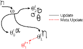
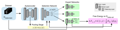
Figure 1: Left: The selector assigns the new input encoding to one of the three experts $\theta_{0}$, $\theta_{1}$, or $\theta_{2}$, depending on the similarity of the input to previous inputs seen by the experts. Right: Our proposed method consists of three main stages. First, we feed the training dataset $D_{\text{train}}$ through a convolutional autoencoder to find a latent representation $z(d_{i})$ for each $d_{i}\in D_{\text{train}}$, which we get by flattening the preceding convolutional layer (“flattening layer”). We apply a pooling function to the resulting set of image embeddings which serves as input to the selection network.

An important concept in decision making is the notion of utility (Von Neumann & Morgenstern, 2007), where an agent picks an action $a_{x}^{*}\in\mathcal{A}$ such that it maximizes their utility in some context $s\in\mathcal{S}$, i.e.,  $a^{*}_{x}=\operatorname*{arg\,max}_{a}\mathbf{U}(x,a)$, where the utility is a function $\mathbf{U}(x,a)$ and the states distribution $p(s)$ is known and fixed. Trying to solve this optimization problem naïvely leads to an exhaustive search over all possible $(a,x)$ pairs, which is in general a prohibitive strategy. Instead of finding an optimal strategy, a bounded-rational decision-maker optimally trades off expected utility and the processing costs required to adapt. In this study we consider the information-theoretic free-energy principle (Ortega & Braun, 2013) of bounded rationality, where an upper bound on the Kullback-Leibler divergence $\operatorname{\text{D}_{\text{KL}}}(p(a|x)||p(a))=\sum_{a}{p(a|x)\log{\frac{p(a|x)}{p(a)}}}$ between the agent’s prior distribution $p(a)$ and the posterior policy $p(a|x)$ model the decision-maker’s resources, resulting in the following constrained optimization problem:

$$\max_{p(a|x)}\sum_{x,a}p(x){p(a|x)\mathbf{U}(x,a)}$$ (1)

$$\text{ s.t. }\mathbb{E}_{p(x)}\left[\operatorname{\text{D}_{\text{KL}}}(p(a|x)||p(a))\right]\leq\text{B}.$$ (2)

This constraint defines a regularization on $p(a|x)$. We can transform this into an unconstrained variational problem by introducing a Lagrange multiplier $\beta\in\mathbb{R}^{+}$:

$$\max_{p(a|x}\mathbb{E}_{p(x|a)}\left[\mathbf{U}(x,a)\right]-\frac{1}{\beta}\mathbb{E}_{p(x)}\left[\operatorname{\text{D}_{\text{KL}}}(p(a|x)||p(a))\right].$$ (3)

For $\beta\rightarrow\infty$ we recover the maximum utility solution and for $\beta\rightarrow 0$ the agent can only act according to the prior. The optimal prior in this case is the marginal $p(a)=\sum_{x\in X}{p(x)p(a|x)}$ (Ortega & Braun, 2013).

Aggregating bounded-rational agents by a selection policy allows for solving optimization problems that exceed the capabilities of the individual decision-makers (Genewein et al., 2015). To achieve this, the search space is split into partitions such that each partition can be solved by a decision-maker. A two-stage mechanism is introduced: The first stage is an expert selection policy $p(m|x)$ that chooses an expert $m$ given a state $x$ and the second stage chooses an action according to the expert’s posterior policy $p(a|x,m)$. The optimization problem given by Equation (3) can be extended to incorporate a trade-off between computational costs and utility in both stages:

$$\max_{p(a|x,m),p(m|x)}\operatorname{\mathbb{E}}[\mathbf{U}(x,a)]-\frac{1}{\beta_{1}}I(X;M)-\frac{1}{\beta_{2}}I(A;X|M)$$ (4)

where $\beta_{1}$ is the resource parameter for the expert selection stage and $\beta_{2}$ for the experts. $I(\cdot;\cdot)$ is the mutual information between the two random variables. To measure a decision-maker’s performance on terms of the utility vs.  cost trade off we use the free-energy difference defined as

$$\operatorname{\Delta\text{F}_{\text{par}}}=\operatorname{\mathbb{E}}_{p}[\mathbf{U}]-\frac{1}{\beta}\operatorname{\text{D}_{\text{KL}}}(p||q),$$ (5)

where $p$ is the posterior and $q$ the decision-maker’s prior policy. The marginal distribution $p(a|x)$ defines a mixture-of-experts (Jordan & Jacobs, 1994; Jacobs et al., 1991) policy given by the posterior distributions $p(a|s,m)$ weighted by the responsibilities determined by the Bayesian posterior $p(x|m)$. Note that $p(x|m)$ is not determined by a given likelihood model, but is the result of the optimization process (4).

3 Meta Learning

We can divide Meta-learning algorithms roughly into Metric-Learning (Koch et al., 2015; Vinyals et al., 2016; Snell et al., 2017), Optimizer Learning (Ravi & Larochelle, 2017; Finn et al., 2017; Zintgraf et al., 2018; Rothfuss et al., 2018), and Task Decomposition Models (Lan et al., 2019; Vezhnevets et al., 2019). Our approach depicted in Figure 1 can be seen as a member of the latter group.

3.1 Meta Supervised Learning

In a supervised learning task we are usually interested in a dataset consisting of multiple input and output pairs $D=\{(x_{i},y_{i})\}^{N}_{i=1}$ and the learner’s task is to find a function $f(x)$ that maps from input to output, for example through a deep neural network. To do this, we split the dataset into training and test sets and fit a set of parameters $\theta$ on the training data and evaluate on test data using the learned function $f_{\theta}(x)$. In meta-learning, we are instead working with meta-datasets $\mathcal{D}$, each containing regular datasets split into training and test sets. We thus have different sets for meta-training, meta-validation, and meta-test, i.e.,  $\mathcal{D}=\{D_{\text{train}},D_{\text{val}},D_{\text{test}}\}$. The goal is to train a learning procedure (the meta-learner) that can take as input one of its training sets $D_{\text{train}}$ and produce a classifier (the learner) that achieves low prediction error on its corresponding test set $D_{\text{test}}$. The meta-learning is then updated using performance measure based the learner’s performance on $D_{\text{val}}$. This may not always be the case, but our work (among others, e.g.,  (Finn et al., 2017)) follow this paradigm. The rationale being that the meta-learner is trained such that it implicitly optimizes the base learner’s generalization capabilities.

3.2 Meta Reinforcement Learning

First, we give a short introduction to reinforcement learning in general, and then we show how this definition can be extended to meta reinforcement learning problems. We model sequential decision problems by defining a Markov Decision Process as a tuple $(\mathcal{S},\mathcal{A},P,r)$, where $\mathcal{S}$ is the set of states, $\mathcal{A}$ the set of actions, $P:\mathcal{S}\times\mathcal{A}\times\mathcal{S}\rightarrow[0,1]$ is the transition probability, and $r:\mathcal{S}\times\mathcal{A}\rightarrow\mathbb{R}$ is a reward function. The aim is to find the parameter $\theta$ of a policy $\pi_{\theta}$ that maximizes the expected reward:

$$\theta^{*}=\operatorname*{arg\,max}_{\theta}\underbrace{\mathbb{E}_{\pi_{\theta}}\left[\sum_{t=0}^{\infty}r(s_{t},a_{t})\right]}_{J(\pi_{\theta})}.$$ (6)

We define $r(\tau)=\sum_{t=0}^{\infty}r(s_{t},a_{t})$ as the cumulative reward of trajectory $\tau=\{(s_{t},a_{t})\}_{i=0}^{\infty}$, which is sampled by acting according to the policy $\pi$, i.e.,  $(s,a)\sim\pi(\cdot|s),$ and $s_{t+1}\sim P(\cdot|s_{t},a_{t})$. We model learning in this environment as reinforcement learning (Sutton & Barto, 2018), where an agent interacts with an environment over some (discrete) time steps $t$. At each time step $t$, the agent finds itself in a state $s_{t}$ and selects an action $a_{t}$ according to the policy $\pi(a_{t}|s_{t})$. In return, the environment transitions to the next state $s_{t+1}$ and generates a scalar reward $r_{t}$. This process continues until the agent reaches a terminal state after which the process restarts. The goal of the agent is to maximize the expected return from each state $s_{t}$, which is typically defined as the infinite horizon discounted sum of the rewards.

In meta reinforcement learning the problem is given by a set of tasks $t_{i}\in T$, where MDP $t_{i}=(\mathcal{S},\mathcal{A},P_{i},r_{i})$ define tasks $t_{i}$ as described earlier. We are now interested in finding a set of policies $\Theta$ that maximizes the average cumulative reward across all tasks in $T$ and generalizes well to new tasks sampled from a different set of tasks $T^{\prime}$.

4 Expert Networks for Meta-Learning

Algorithm 1 Expert Networks for Supervised Meta-Learning.

1:  Input: Data Distribution $p(\mathcal{D})$, number of samples $K$, batch-size $M$, training episodes $N$ 

2:  Hyper-parameters: resource parameters $\beta_{1}$, $\beta_{2}$, learning rates $\eta_{x}$, $\eta_{x}$ for selector and experts 

3:  Initialize parameters $\theta,\vartheta$ 

4:  for $i$ = 0, 1, 2, …, $N$ do

5:     Sample batch of $M$ datasets $D_{i}\thicksim p(\mathcal{D})$, each consisting of a training dataset $D_{\text{{meta-train}}}$ and a meta-validation dataset  $D_{\text{{meta-val}}}$ with $2K$ samples each  

6:     for $D\in D_{i}$ do

7:        Find Latent Embedding $z(D_{\text{{meta-train}}})$  

8:        Select expert $m\thicksim p_{\theta}(m|z(D_{\text{{meta-train}}})$  

9:        Compute $\hat{f}(m,D_{\text{val}})$  

10:     end for 

11:     Update selection parameters $\theta$ with $\hat{f}(m,D_{\text{val}})$  

12:     Update Autoencoder with positive samples in $D_{i}$  

13:     Update experts $m$ with assigned $D_{\text{{meta-train}}}$ 

14:  end for 

15:  return $\theta$, $\vartheta$ 

Information-theoretic bounded rationality postulates that hierarchies and abstractions emerge when agents have only limited access to computational resources (Genewein et al., 2015), e.g.,  limited sampling complexity (Hihn et al., 2018) or limited representational power (Hihn et al., 2019). We will show that forming such abstractions equips an agent with the ability of learning the underlying problem structure and thus enables learning of unseen but similar concepts. The method we propose comes out of a unified optimization principle and has the following important features:

1. A regularization mechanism to enforce the emergence of expert policies.

2. A task compression mechanism to extract relevant task information.

3. A selection mechanism to find the most efficient expert for a given task.

4. A regularization mechanism to improve generalization capabilities.

4.1 Latent Task Embeddings

Note that the selector assigns a complete dataset to an expert and that this can be seen as a meta-learning task, as described in (Ravi & Larochelle, 2017). To do so, we must find a feature vector $z(d)$ of the dataset $d$. This feature vector must fulfill the following desiderata: 1) invariance against permutation of data points in $d$, 2) high representational capacity, 3) efficient computability, and 4) constant dimensionality regardless of sample size $K$. In the following we propose such features for image classification, regression, and reinforcement learning problems.

For image classification we propose to pass the positive images in the dataset through a convolutional autoencoder and use the outputs of the bottleneck layer. Convolutional Autoencoders are generative models that learn to reconstruct their inputs by minimizing the Mean-Squared-Error between the input and the reconstructed image (see e.g.,  (Chen et al., 2019)). In this way we get similar embeddings $z(d)$ for similar inputs belonging to the same class. The latent representation is computed for each positive sample in $d$ and then passed through a pooling function $h(z(d))$ to find a single embedding for the complete dataset–see figure 1 for an overview of our proposed model. While in principle functions such as mean, max, and min can be used, we found that max-pooling yields the best results. The authors of (Yao et al., 2019) propose a similar feature set.

For regression we define a similar feature vector. We transform the $K$ training data points into a feature vector $z(d)$ by binning the points into $N$ bins according to their $x$ value and collecting the $y$ value. If more than one point falls into the same bin, we average the $y$ values, thus providing invariance against the order of the data points in $D_{\text{train}}$. We use this feature vector to assign each data set to an expert according to $p_{\theta}(x|z(d))$.

In the reinforcement learning setting we use a dynamic recurrent neural network (RNN) with LSTM units (Hochreiter & Schmidhuber, 1997) to classify trajectories. We feed the RNN with $(s_{t},a_{t},r_{t},t)$ tuples to describe the underlying Markov Decision Process describing the task. At $t=0$ we sample the expert $x$ according to the learned prior distribution $p(x)$, as there is no information available so far. The authors of (Lan et al., 2019) propose a similar feature set.

4.2 Specialization in Supervised Learning

Combining multiple experts can often be beneficial (Kuncheva, 2004), e.g. in Mixture-of-Experts (Yuksel et al., 2012) or Multiple Classifier Systems (Bellmann et al., 2018). Our method can be interpreted as a member of this family of algorithms.

We define the utility as the negative prediction loss, i.e. $U(f_{x}(d),y)=-\mathcal{L}(f_{x}(d),y)$, where $f_{x}(d)$ is the prediction of the expert $x$ given the input data point $d$ (in the following we will use the shorthand $\hat{y}_{x}$) and $y$ is the ground truth. We define the cross-entropy loss $\mathcal{L}(\hat{y}_{x},y,)=-\sum_{i}y_{i}\log\hat{y_{i}}_{x}$ as a performance measure for classification and the mean squared error $\mathcal{L}(\hat{y}_{x},y)=\sum_{i}(\hat{y}_{i}-y_{i})^{2}$ for regression. The objective for expert selection thus is given by

$$\max_{\theta}\operatorname{\mathbb{E}}_{p_{\theta}(x|d)}\left[\hat{f}-\frac{1}{\beta_{1}}\log\frac{p_{\theta}(x|d)}{p(x)}\right],$$ (7)

where $\hat{f}=\mathbb{E}_{p_{\vartheta}(\hat{y}_{x}|x,s)}\left[-\mathcal{L}(\hat{y}_{x},y)-\frac{1}{\beta_{2}}\log\frac{p_{\vartheta}(\hat{y}_{x}|s,x)}{p(\hat{y}_{x}|x)}\right]$, i.e. the free energy of the expert and $\theta,\vartheta$ are the parameters of the selection policy and the expert policies, respectively. Analogously, the action selection objective for each expert $x$ is defined by

$$\max_{\vartheta}\operatorname{\mathbb{E}}_{p_{\vartheta}(\hat{y}_{x}|x,s)}\left[-\mathcal{L}(\hat{y}_{x},y)-\frac{1}{\beta_{2}}\log\frac{p_{\vartheta}(\hat{y}_{x}|s,x)}{p_{(}\hat{y}_{x}|x)}\right].$$ (8)

This regularization technique can be seen as a form of output regularization (Pereyra et al., 2017).

4.3 Specialization in Reinforcement Learning

Algorithm 2 Expert Networks for Meta-Reinforcement Learning.

1:  Input: Environment Distributions $p(T)$ and $p(T^{\prime})$, number of roll-outs $K$, batch-size $M$, training episodes $N$, number of tuples $L$ used for expert selection 

2:  Hyper-parameters: resource parameters $\beta_{1}$, $\beta_{2}$, learning rates $\eta_{x}$, $\eta_{x}$ for selector and experts 

3:  Initialize parameters $\theta,\vartheta$ 

4:  for $i$ = 1, 2, 3, …, $N$ do

5:     Sample batch of $M$ environments $E_{i}^{\text{train}}\thicksim p(T)$ and $E_{i}^{\text{val}}\thicksim p(T^{\prime})$ 

6:     for $E\in E_{i}^{\text{train}}$ do

7:        for $k$ = 1, 2, 3, …, $K$ do

8:           Collect $\tau=\{(x_{t},a_{t},r_{t},t)\}_{t=1}^{L}$ tuples by following random expert  

9:           Select expert $m\thicksim p_{\theta}(m|\tau)$ with RNN policy  

10:           Collect trajectory $\tau_{k}=\{(x_{t},a_{t},r_{t},t)\}_{t=L}^{T}$ by following $p_{\vartheta}(a|x,m)$

11:        end for 

12:        Compute $F_{t}=\sum_{l=0}^{T}\gamma^{l}f(x_{t+l},m_{t+l},a_{t+l})$ for trajectories $\tau$ 

13:        where $f(x,m,a)=r_{\text{train}}(x,a)-\frac{1}{\beta_{2}}\log\frac{p_{\vartheta}(a|x,m)}{p(a|m)}$.

14:     end for 

15:     Compute $\bar{F}_{t}=\sum_{l=0}^{T}\gamma^{l}\bar{f}(x_{t+l},m_{t+l})$ with  

16:     $\bar{f}(x,m)=\mathbb{E}_{p_{\vartheta}(a|x,m)}\left[r_{\text{val}}(x,a)-\frac{1}{\beta_{2}}\log\frac{p(a|x,m)}{p(a|m)}\right]$  

17:     Update selection parameters $\theta$ with $\bar{F}$ collected in batch $i$  

18:     Update experts $m$ with roll-outs collected in batch $i$ 

19:  end for 

20:  return $\theta$, $\vartheta$ 

In the following we will derive our algorithm for specialization in hierarchical reinforcement learning agents. Note that in the reinforcement learning setup the reward function $r(x,a)$ defines the utility $\mathbf{U}(x,a)$. In maximum entropy RL (see e.g.,  Haarnoja et al.  (2017) (Haarnoja et al., 2017)) the regularization penalizes deviation from a fixed uniformly distributed prior, but in a more general setting we can discourage deviation from an arbitrary prior policy by optimizing for:

$$\max_{p}\mathbb{E}_{p}\left[\sum_{t=0}^{\infty}\gamma^{t}\left(r(x_{t},a_{t})-\frac{1}{\beta}\log\frac{p(a_{t}|x_{t})}{p(a)}\right)\right],$$ (9)

where $\beta$ trades off between reward and entropy, such that $\beta\rightarrow\infty$ recovers the standard RL value function and $\beta\rightarrow 0$ recovers the value function under a random policy.

To optimize the objective (9) we define two separate kinds of value function, $V_{\phi}$ for the selector and one value function $V_{\varphi}$ for each expert. Thus, each expert is an actor-critic with separate actor and critic networks. Similarly, the selector has an actor-critic architecture, where the actor network selects experts and the critic learns to predict the expected free energy of the experts depending on a state variable. The selector’s policy is represented by $p_{\theta}$, while each expert’s policy is represented by a distribution $p_{\vartheta}$.

In standard reinforcement learning a common technique to update a parametric policy representation $p_{\omega}(a|x)$ with parameters $\omega$, is to use policy gradients that optimize the cumulative reward $J(\omega)=\mathbb{E}\left[p_{\omega}(a|x)V_{\psi}(x)\right]$ expected under the critic’s prediction $V_{\psi}(x)$, by following the gradient $\nabla_{\omega}J(\omega)=\mathbb{E}\left[\nabla_{\omega}\log p_{\omega}(a|x)V_{\psi}(x)\right].$ This policy gradient formulation (Sutton et al., 2000) is prone to producing high variance gradients. A common technique to reduce the variance is to formulate the updates using the advantage function instead of the reward (Arulkumaran et al., 2017). The advantage function $A(a,x)$ is a measure of how well a certain action $a$ performs in a state $x$ compared to the average performance in that state, i.e., $A(a,x)=Q(x,a)-V_{\psi}(x)$. Here, $V(x)$ is the value function and is a measure of how well the agent performs in state $x$, and $Q(x,a)$ is an estimate of the cumulative reward achieved in state $x$ when the agent executes action $a$. Instead of learning the value and the Q function, we can approximate the advantage function solely based on the critic’s estimate $V_{\psi}(x)$ by noting that $Q(x_{t},a_{t})\approx r(x_{t},a_{t})+\gamma V_{\psi}(x_{t+1})$. Similar to the standard policy update based on the advantage function, the expert selection stage can be formulated by optimizing the expected advantage $\mathbb{E}_{p_{\vartheta}(a|x,m)}\left[A_{m}(x,a)\right]$ for expert $m$ with

$$A_{m}(x_{t},a_{t})=f(x_{t},m,a_{t})+\gamma V_{\varphi}(x_{t+1})-V_{\varphi}(x_{t}).$$ (10)

Accordingly, we can define an expected advantage function $\mathbb{E}\left[p_{\theta}(m|x)\bar{A}(x,m)\right]$ for the selector with

$$\bar{A}(x,m)=\mathbb{E}_{p_{\vartheta}(a|x,m)}\left[A_{m}(x,a)\right],$$ (11)

where $m_{t}$ denotes the expert $m$ selected at time $t$. We estimate the double expectation by Monte Carlo sampling, where in practice we use a single $(x,m,a)$ tuple for $\hat{f}(x,m)$, which enables us to employ our algorithm in an on-line optimization fashion.

Omniglot Few-Shot
	One Conv. Block Baselines			Methods
	Pre-Training	MAML	Matching Nets	MAML	Matching Nets
K	% Acc	% Acc	% Acc	% Acc	% Acc
1	50.6 ($\pm$ 0.03)	81.2 ($\pm$ 0.03)	52.7 ($\pm$ 0.05)	95.2 ($\pm$ 0.03)	95.0 ($\pm$ 0.01)
5	54.1 ($\pm$ 0.09)	88.0 ($\pm$ 0.01)	55.3 ($\pm$ 0.04)	99.0 ($\pm$ 0.01)	98.7 ($\pm$ 0.01)
10	55.8 ($\pm$ 0.02)	89.2 ($\pm$ 0.01)	60.9 ($\pm$ 0.06)	99.2 ($\pm$ 0.01)	99.4 ($\pm$ 0.01)
Our Method
Number of Experts
	2		4
	% Acc	I(M;X)	% Acc	I(M;X)
1	66.4 ($\pm$ 0.02)	0.99 ($\pm$ 0.01)	75.8 ($\pm$ 0.02)	1.96 ($\pm$ 0.01)
5	67.3 ($\pm$ 0.01)	0.93 ($\pm$ 0.01)	75.5 ($\pm$ 0.01)	1.95 ($\pm$ 0.10)
10	76.2 ($\pm$ 0.04)	0.95 ($\pm$ 0.30)	86.7 ($\pm$ 0.01)	1.90 ($\pm$ 0.03)
	8		16
	% Acc	I(M;X)	% Acc	I(M;X)
1	77.3 ($\pm$ 0.01)	2.5 ($\pm$ 0.02)	82.8 ($\pm$ 0.01)	3.2 ($\pm$ 0.03)
5	78.4 ($\pm$ 0.01)	2.7 ($\pm$ 0.01)	85.2 ($\pm$ 0.01)	3.3 ($\pm$ 0.02)
10	90.1 ($\pm$ 0.01)	2.8 ($\pm$ 0.02)	95.9 ($\pm$ 0.01)	3.1 ($\pm$ 0.02)

Table 1: Classification accuracy after 10 gradient steps on the validation data. Adding experts consistently improves performance, obtaining the best results with an ensemble of 16 experts. Pre-training refers to a single expert system trained on the complete dataset. Our method outperforms the pre-training, Matching Nets, and the MAML baseline (see Section 5.1 for experimental details), when the network architecture is reduced to a single convolution block. This corresponds to our expert network architecture. Using the suggested architectures by the respective studies, we achieve classification accuracy $\geq 95\%$.

In the RL setup the reward function $r(x,a)$ defines the utility $\mathbf{U}(x,a)$. To optimize the objective we define value functions, $V_{\phi}$ for the selector and one value function $V_{\varphi}$ for each expert. Thus, the selector and each expert is an actor-critic architecture. We define a discounted free energy as

$$F_{t}=\sum_{l=0}^{T}\gamma^{l}\left(r(x_{t+l},a_{t+l})-\frac{1}{\beta_{2}}\log\frac{p_{\vartheta}(a_{t+l}|x_{t+l},m_{t+l})}{p(a_{t+l}|m_{t+l})}\right),$$ (12)

which we learn through a value function $V_{\varphi}$ for each expert. We define the selector’s discounted free energy

$$\bar{F}_{t}=\sum_{l=0}^{T}\gamma^{l}\bar{f}(x_{t+l},m_{t+l}),$$ (13)

with $\bar{f}(x,m)=\mathbb{E}_{p_{\vartheta}(a|x,m)}[r(x,a)-\frac{1}{\beta_{2}}\log\frac{p_{\vartheta}(a|x,m)}{p(a|m)}]$ that is learned through the selector’s value function $V_{\phi}$. Now let $p_{\theta}(m|x)$ be the selection policy and $p_{\vartheta}(a|x,m)$ the expert policy. The expert selection stage is optimizing the expected advantage $\mathbb{E}\left[p_{\vartheta}(a|x,m)A_{m}(x,a)\right]$ for expert $m$ with

$$A_{m}(x_{t},a_{t})=f(x_{t},m,a_{t})+\gamma V_{\varphi}(x_{t+1})-V_{\varphi}(x_{t}).$$ (14)

Accordingly, we define an expected advantage function $\mathbb{E}\left[p_{\theta}(m|x)\bar{A}(x,m)\right]$ for the selector with

$$\bar{A}(x,m)=\mathbb{E}_{p_{\vartheta}(a|x,m)}\left[A_{m}(x,a)\right].$$ (15)

We find the policy parameters by gradient descent on the objectives.

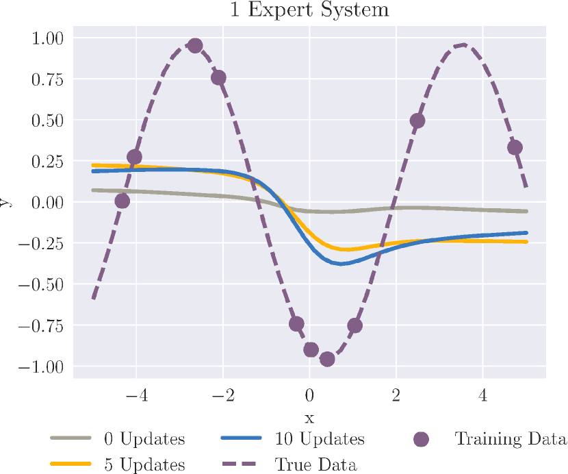
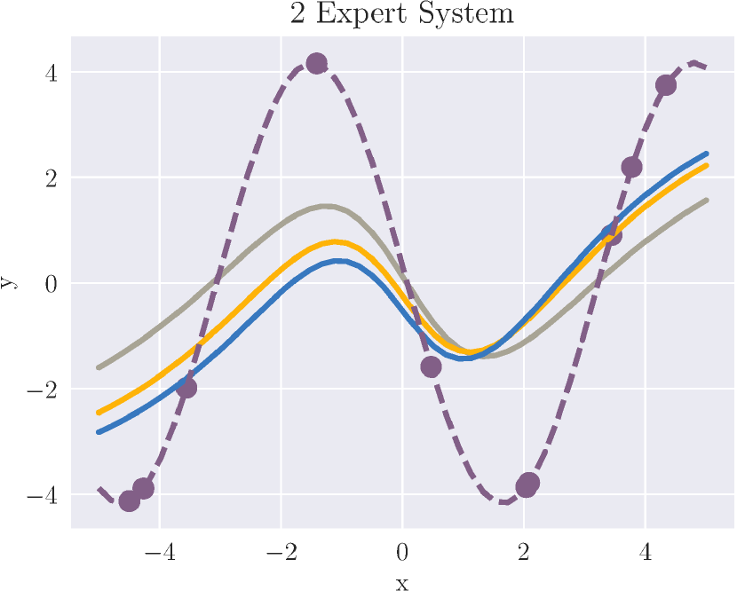
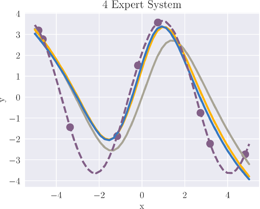
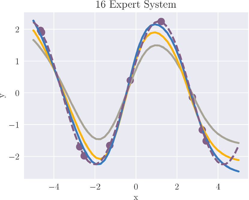
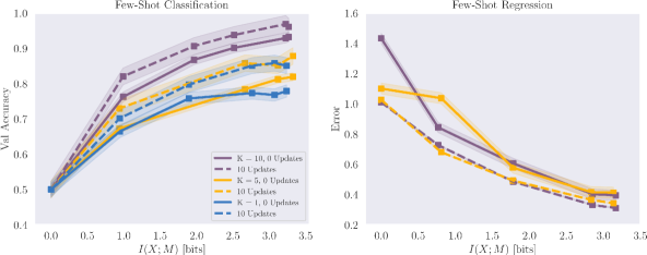
Figure 2: The single expert system is not able to learn the structure of the sine wave, where the two expert can capture the periodic structure. The lower figure shows how the error decreases as we add more experts in the classification and regression setting, indicating successful specialization and expert selection.

5 Results

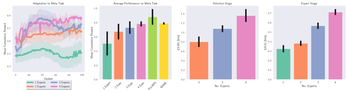
Figure 3: In each Meta-Update Step we sample $N$ tasks from the training task set $T$ and update the agents. After training we evaluate their performance on a tasks from the meta test set $T^{\prime}$. Rewards are normalized to $[0,1]$ and the episode horizon is 100 time steps. The agent achieves higher reward when adding more experts while the information-processing of the selection and of the expert stage increases, indicating that the added experts specialize successfully. We achieve comparable results to MAML (Finn et al., 2017) and Proximal Meta-Policy Search (Rothfuss et al., 2018). Shaded areas and error bars represent one standard deviation. In Table 2 in the Appendix we give experimental details.

5.1 Sinusoid Regression

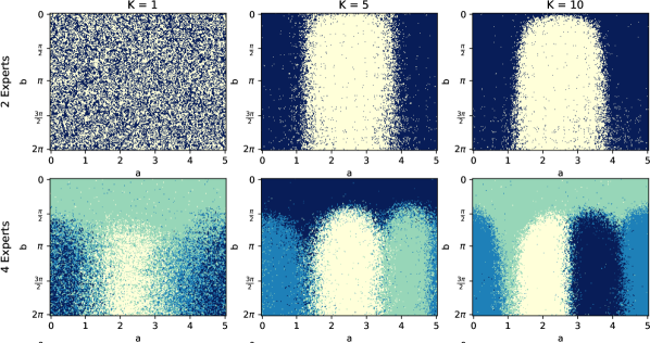
Figure 4: Here we show the soft-partition found by the selection policy for the sine prediction problem, where each color represents an expert. We can see that the selection policy becomes increasingly more precise as we provide more points per dataset to the system.

We adopt this task from (Finn et al., 2017). In this $K$-shot problem, each task consists of learning to predict a function of the form $y=a\cdot\sin(x+b)$, with both $a\in[0.1,5]$ and $b\in[0,2\pi]$ chosen uniformly, and the goal of the learner is to find $y$ given $x$ based on only $K$ pairs of $(x,y)$. Given that the underlying function changes in each iteration it is impossible to solve this problem with a single learner. Our results show that by combing expert networks, we are able to reduce the generalization error iteratively as we add more experts to our system–see Figure 2 where we also show how the system is able to capture the underlying problem structure as we add more experts. In Figure 4 we visualize how the selector’s partition of the problem space looks like. The shape of the emerged clusters indicates that the selection is mainly based on the amplitude $a$ of the current sine function, indicating that from an adaptation point-of-view it is more efficient to group sine functions based on amplitude $a$ instead of phase $b$. We can also see that an expert specializes on the low values for $b$ as it covers the upper region of the $a\times b$ space. The selection network splits this region among multiple experts if we increase the set of experts to 8 or more.

5.2 Few-Shot Classification

The Omniglot dataset (Lake et al., 2011) consists of over 1600 characters from 50 alphabets. As each character has only 20 samples each drawn by a different person, this forms a challenging meta-learning benchmark.

The selection policy now selects experts based on their free-energy that is computed over datasets $D_{\text{val}}$ and the selection policy depends on the training datasets $D_{\text{train}}$:

$$\max_{\theta}\operatorname{\mathbb{E}}_{p_{\theta}(m|D_{\text{train}})}\left[\hat{f}(m,D_{\text{val}})-\frac{1}{\beta_{1}}\log\frac{p_{\theta}(m|D_{\text{train}})}{p(m)}\right],$$ (16)

where $\hat{f}(m,D_{\text{val}})\coloneqq\mathbb{E}_{p_{\vartheta}(\hat{y}|m,x)}\big{[}-\mathcal{L}(\hat{y},y)-\frac{1}{\beta_{2}}\log\frac{p_{\vartheta}(\hat{y}|x,m)}{p(\hat{y}|m)}\big{]}$ is the free energy of expert $m$ on dataset $D_{\text{val}}$, $\mathcal{L}(\hat{y},y)$ is loss function, and $(x,y)\in D_{\text{val}}$. The experts optimize their free energy objective on the training dataset $D_{\text{train}}$ defined by

$$\max_{\vartheta}\operatorname{\mathbb{E}}_{p_{\vartheta}(\hat{y}|m,x)}\left[-\mathcal{L}(\hat{y},y)-\frac{1}{\beta_{2}}\log\frac{p_{\vartheta}(\hat{y}|x,m)}{p(\hat{y}|m)}\right],$$ (17)

where $(x,y)\in D_{\text{train}}$.

We train the learner on a subset of the dataset ($\approx 80\%$, i.e.,  $\approx$ 1300 classes) and evaluate the remaining $\approx 300$ classes, thus investigating the generalization. In each training episode we build the datasets $D_{\text{train}}$ and $D_{\text{val}}$ by selecting a target class $c_{t}$ and sampling $K$ positive and $K$ negative samples. To generate negative samples, we draw $K$ images randomly out of the remaining $N-1$ classes. We present the selection network with the feature presentation of the $K$ positive training samples (see Figure 1), but evaluate the experts’ performance on the $2K$ test samples in $D_{\text{val}}$. In this way, the free energy of the experts becomes a generalization measure. Using this optimization scheme, we train the networks to become experts in recognizing a subset of classes. After a proper expert is selected we train that expert using the $2K$ samples from the training dataset.

We consider three experimental setups: 1) how does a learner with only a single hidden layer perform when trained nïvely compared to with sophisticated methods such as MAML (Finn et al., 2017) and Matching Nets (Vinyals et al., 2016) as a baseline? 2) does the system benefit from adding more experts and if so, at what rate? and 3) how does our method compare to the aforementioned algorithms? Regarding 1) we note that introducing constraints by reducing the representational power of the models does not facilitate specialization is it would by explicit information-processing constraints. In the bottom row of Figure 2 we address question 2). We can interpret this curve as the rate-utility curve showing the trade-off between information processing and expected utility (transparent area represents one standard deviation), where increasing $I(X;M)$ improves adaptation. The improvement gain grows logarithmically, which is consistent with what rate-distortion theory would suggest. In Table 1 we present empirical results addressing question 3).

5.3 Meta Reinforcement Learning

We create a set of RL tasks by sampling the parameters for the Inverted Double Pendulum problem (Sutton, 1996) implemented in OpenAI Gym (Brockman et al., 2016), where the task is to balance a two-link pendulum in an upward position. We modify inertia, motor torques, reward function, goal position and invert the control signal – see Table 2 for details. We build the meta task set $T^{\prime}$ on the same environment, but change the parameter distribution and range, providing new but similar reinforcement learning problems. During training, we sample $M$ environments in each episode and perform updates as described earlier. During evaluation, we measure the system’s performance on tasks sampled from $T^{\prime}$– see results in Figure 3, where we can see improving performance as more experts are added and the increasing mutual information in the selection stage indicates precise partitioning.

The expert policies are trained on the meta-training environment policies, but evaluated on unseen but similar validation environments. In this setting we define the discounted free energy $\bar{F}_{t}$ with

$$\bar{f}(x,m)=\mathbb{E}_{p_{\vartheta}(a|x,m)}\left[r_{\text{val}}(x,a)-\frac{1}{\beta_{2}}\log\frac{p(a|x,m)}{p(a|m)}\right],$$

where $r_{\text{val}}$ is a reward function defined by a validation environment (see Figure 3 for details).

6 Related Work

The hierarchical structure we employ is related to Mixture of Experts (MoE) models. (Jacobs et al., 1991; Jordan & Jacobs, 1994) introduced MoE as tree structured models for complex classification and regression problems, where the underlying approach is a divide and conquer paradigm. As in our approach, three main building blocks define MoEs: gates, experts, and a probabilistic weighting to combine expert predictions. Learning proceeds by finding a soft partitioning of the input space and assigning partitions to experts performing well on the partition. In this setting, the model response is then a sum of the experts’ outputs, weighted by how confident the gate is in the expert’s opinion (see (Yuksel et al., 2012) for an overview). This paradigm has seen recent interest in the field of machine learning, see e.g.,  (Aljundi et al., 2017; Rosenbaum et al., 2019; Jerfel et al., 2019; Shazeer et al., 2017). The approach we propose allows learning such models, but also has applications to more general decision-making settings such as reinforcement learning.

Our approach belongs to a wider class of models that use information constraints for regularization to deal more efficiently with learning and decision-making problems (Martius et al., 2013; Leibfried et al., 2017; Grau-Moya et al., 2017; Achiam et al., 2017; Hihn et al., 2018; Grau-Moya et al., 2019). One such prominent approach is Trust Region Policy Optimization (TRPO) (Schulman et al., 2015). The main idea is to constrain each update step to a trust region around the current state of the system. This region is defined by $\operatorname{\text{D}_{\text{KL}}}(\pi_{\text{new}}||\pi_{\text{old}})$ between the old policy and the new policy, providing a theoretic monotonic policy improvement guarantee. In our approach we define this region by $\operatorname{\text{D}_{\text{KL}}}$ between the agent’s posterior and prior policy, thus allowing to learn this region and to adapt it over time. This basic idea has been extend to meta-learning by (Rothfuss et al., 2018), which we use to compare our method against in meta-rl experiments.

Most other methods for meta-learning such as the work of (Finn et al., 2017) and (Ravi & Larochelle, 2017) find an initial parametrization of a single learner, such that the agent can adapt quickly to new problems. This initialization represents prior knowledge and can be regarded as an abstraction over related tasks and our method takes this idea one step further by finding a possibly disjunct set of such compressed task properties. Another way of thinking of such abstractions by lossy compression is to go from a task-specific posterior to a task-agnostic prior strategy. By having a set of priors the task specific information is available more locally then with a single prior, as in MAML (Finn et al., 2017) and the work of (Ravi & Larochelle, 2017). In principle, this can help to adapt within fewer iterations. Thus our method can be seen as the general case of such monolithic meta-learning algorithms. Instead of learning similarities within a problem, we can also try to learn similarities between different problems (e.g.,  different classification datasets), as is described in the work of (Yao et al., 2019). In this way, the partitioning is governed by different tasks, where our study however focuses on discovering meta-information within the same task family, where the meta-partitioning is determined solely by the optimization process and can thus potentially discover unknown dynamics and relations within a task family.

7 Discussion

We have introduced and evaluated a novel hierarchical information-theoretic approach to meta-learning. In particular, we leveraged an information-theoretic approach to bounded rationality. Although our method is widely applicable, it suffers from low sample efficiency in the RL domain. A research direction would be to combine our system with model-based RL which is known to improve sample efficiency. Another research direction would be to investigate the performance of our system in continual adaption tasks, such as in (Yao et al., 2019). Another limitation is the restriction to binary meta classification tasks, which we leave for feature work.

The results show that our method can identify sub-regions of the problem set and solve them efficiently with expert networks. In effect, this equips the system with initializations covering the problem space and thus enables it to adapt quickly to new but similar tasks. To reliably identify such tasks, we have proposed feature extraction methods for classification, regression, and reinforcement learning, that could be simply be replaced and improved in future work. The strength of our model is that it follows from simple principles that can be applied to a large range of problems. Moreover, the system performance can be interpreted in terms of the information processing of the selection stage and the expert decision-makers. We have shown empirically that our method achieves results comparable to recent meta-learning algorithms, such as MAML (Finn et al., 2017), Matching Nets (Vinyals et al., 2016), and Proximal Meta-Policy Search (Rothfuss et al., 2018).

Acknowledgments

This work was supported by the European Research Council Starting Grant BRISC, ERC-STG-2015, Project ID 678082.

Appendix

Few-Shot Classification Experimental details: We followed the design of (Vinyals et al., 2016) but reduce the number of blocks to one. We used a single convolutional block consisting of 32 3$\times$3 filters with strided convolutions followed by a batch normalization layer and a ReLu non-linearity. During training we used a meta-batch size of 16. The convolutional autoencoder is a 3 layer network consisting of 16, 16, and 4 filters each with size 3$\times$3 with strided convolutions followed by a leaky ReLu non-linearity. The layers are mirrored by de-convolotional layers to reconstruct the image. This results in an image embedding with dimensionality 64. The selection network is a two layer network with 32 units each, followed by a ReLu non-linearity, a dropout layer (Srivastava et al., 2014) per layer. We augment the dataset by rotating each image in 90, 180, and 270 degrees resulting in 80 images per class. We also normalize the images two be in (0,1) range. We evaluate our method by resetting the system to the state after training and allow for 10 gradient updates and report the final accuracy. To evaluate MAML on 2-way $N$-shot omniglot dataset we used a inner learning rate of $\alpha=0.05$ and one inner update step per iteration for all settings. We used a single convolutional block followed by a fully connected layer with 64 units and a ReLU non-linearity. Note, that we reduce the number of layers to make the tests comparable. Using the suggested architectures by (Finn et al., 2017) we achieve classification accuracy $\geq 95\%$. To generate this figure, we ran 10-fold cross-validation on the whole dataset and show the averaged performance metric and the standard-deviation across the folds. In both settings, ”0 bits” corresponds to a single expert, i.e.,  a single neural network trained on the task.

Meta-RL Experimental details: The selector’s actor and critic net are build of RNNs with 200 hidden units each. The critic is trained to minimize the Huber loss between the prediction and the cumulative reward. The experts are two layer networks with 64 units each followed by ReLu non-linearities and used to learn the parameters of a Gaussian distribution. The critics have the same architecture (except for the output dimensionality). The control signal $a$ is continuous in the interval [-1,1] and is generated by neural network that outputs $\mu$ and $\log(\sigma)$ of a gaussian. The action is then sampled by re-parameterizing the distribution to $p(a)=\mu+\exp(\sigma)\epsilon$, where $\epsilon\thicksim\mathcal{N}(0,1)$, so that the distribution is differentiable w.r.t to the network outputs. We average the results over 10 random seeds and trained for 1000 episodes each with a batch of 64 environments.

	Task Distribution
Paramater	$T$	$T^{\prime}$
Distance Penalty	[$10^{-3},10^{-1}$]	[$10^{-3},10^{-2}$]
Goal Position	[0.3, 0.4]	[0, 3]
Start Position	[-0.15, 0.15]	[-0.25, 0.25]
Motor Torques	$[0,5]$	$[0,3]$
Inverted Control	$p=0.5$	$p=0.5$
Gravity	[0.01, 4.9]	[4.9, 9.8]
Motor Actuation	[185, 215]	[175, 225]

Table 2: Environment Parameters for the Meta-RL Setting.

Regression Experimental details: For regression we use a two layer selection network with 16 units each followed by tanh non-linearities. The experts are shallow neural networks with a single hidden layer that learn log-variance and mean of a Gaussian distribution which they use for prediction. We use the “Huber Loss” instead of MSE as it is more robust (Balasundaram & Meena, 2019). We optimize all networks using Adam (Kingma & Ba, 2014).

References

- Achiam et al. (2017) Achiam, J., Held, D., Tamar, A., and Abbeel, P. Constrained policy optimization. In Proceedings of the 34th International Conference on Machine Learning-Volume 70, pp. 22–31. JMLR. org, 2017.
- Aljundi et al. (2017) Aljundi, R., Chakravarty, P., and Tuytelaars, T. Expert gate: Lifelong learning with a network of experts. In Proceedings of the IEEE Conference on Computer Vision and Pattern Recognition, pp. 3366–3375, 2017.
- Arulkumaran et al. (2017) Arulkumaran, K., Deisenroth, M. P., Brundage, M., and Bharath, A. A. Deep reinforcement learning: A brief survey. IEEE Signal Processing Magazine, 34(6):26–38, 2017.
- Balasundaram & Meena (2019) Balasundaram, S. and Meena, Y. Robust support vector regression in primal with asymmetric huber loss. Neural Processing Letters, 49(3):1399–1431, 2019.
- Bellmann et al. (2018) Bellmann, P., Thiam, P., and Schwenker, F. Multi-classifier-systems: Architectures, algorithms and applications. In Computational Intelligence for Pattern Recognition, pp. 83–113. Springer, 2018.
- Botvinick et al. (2019) Botvinick, M., Ritter, S., Wang, J. X., Kurth-Nelson, Z., Blundell, C., and Hassabis, D. Reinforcement learning, fast and slow. Trends in cognitive sciences, 2019.
- Braun et al. (2009) Braun, D. A., Aertsen, A., Wolpert, D. M., and Mehring, C. Motor task variation induces structural learning. Current Biology, 19(4):352–357, 2009.
- Brockman et al. (2016) Brockman, G., Cheung, V., Pettersson, L., Schneider, J., Schulman, J., Tang, J., and Zaremba, W. Openai gym. arXiv preprint arXiv:1606.01540, 2016.
- Caruana (1997) Caruana, R. Multitask learning. Machine learning, 28(1):41–75, 1997.
- Chen et al. (2019) Chen, W.-Y., Liu, Y.-C., Kira, Z., Wang, Y.-C. F., and Huang, J.-B. A closer look at few-shot classification. In Proceedings of the International Conference on Representation Learning, 2019.
- Devlin et al. (2018) Devlin, J., Chang, M.-W., Lee, K., and Toutanova, K. Bert: Pre-training of deep bidirectional transformers for language understanding. arXiv preprint arXiv:1810.04805, 2018.
- Finn et al. (2017) Finn, C., Abbeel, P., and Levine, S. Model-agnostic meta-learning for fast adaptation of deep networks. In Proceedings of the 34th International Conference on Machine Learning-Volume 70, pp. 1126–1135. JMLR. org, 2017.
- Genewein et al. (2015) Genewein, T., Leibfried, F., Grau-Moya, J., and Braun, D. A. Bounded rationality, abstraction, and hierarchical decision-making: An information-theoretic optimality principle. Frontiers in Robotics and AI, 2:27, 2015.
- Grau-Moya et al. (2017) Grau-Moya, J., Krüger, M., and Braun, D. A. Non-equilibrium relations for bounded rational decision-making in changing environments. Entropy, 20(1):1, 2017.
- Grau-Moya et al. (2019) Grau-Moya, J., Leibfried, F., and Vrancx, P. Soft q-learning with mutual-information regularization. In Proceedings of the International Conference on Learning Representations, 2019.
- Haarnoja et al. (2017) Haarnoja, T., Tang, H., Abbeel, P., and Levine, S. Reinforcement learning with deep energy-based policies. In Proceedings of the 34th International Conference on Machine Learning-Volume 70, pp. 1352–1361. JMLR. org, 2017.
- Hihn et al. (2018) Hihn, H., Gottwald, S., and Braun, D. A. Bounded rational decision-making with adaptive neural network priors. In IAPR Workshop on Artificial Neural Networks in Pattern Recognition, pp. 213–225. Springer, 2018.
- Hihn et al. (2019) Hihn, H., Gottwald, S., and Braun, D. A. An information-theoretic on-line learning principle for specialization in hierarchical decision-making systems. In Proceedings of the 2019 IEEE Conference on Decision-Making and Control (CDC), 2019.
- Hochreiter & Schmidhuber (1997) Hochreiter, S. and Schmidhuber, J. Long short-term memory. Neural computation, 9(8):1735–1780, 1997.
- Jacobs et al. (1991) Jacobs, R. A., Jordan, M. I., Nowlan, S. J., and Hinton, G. E. Adaptive mixtures of local experts. Neural computation, 3(1):79–87, 1991.
- Jankowski et al. (2011) Jankowski, N., Duch, W., and Grkabczewski, K. Meta-learning in computational intelligence, volume 358. Springer Science & Business Media, 2011.
- Jerfel et al. (2019) Jerfel, G., Grant, E., Griffiths, T., and Heller, K. A. Reconciling meta-learning and continual learning with online mixtures of tasks. In Advances in Neural Information Processing Systems, pp. 9122–9133, 2019.
- Jordan & Jacobs (1994) Jordan, M. I. and Jacobs, R. A. Hierarchical mixtures of experts and the em algorithm. Neural computation, 6(2):181–214, 1994.
- Kingma & Ba (2014) Kingma, D. P. and Ba, J. Adam: A method for stochastic optimization. In Proceedings of the International Conference on Representation Learning, 2014.
- Koch et al. (2015) Koch, G., Zemel, R., and Salakhutdinov, R. Siamese neural networks for one-shot image recognition. In ICML deep learning workshop, volume 2, 2015.
- Kuncheva (2004) Kuncheva, L. I. Combining pattern classifiers: methods and algorithms. John Wiley & Sons, 2004.
- Lake et al. (2011) Lake, B., Salakhutdinov, R., Gross, J., and Tenenbaum, J. One shot learning of simple visual concepts. In Proceedings of the Annual Meeting of the Cognitive Science Society, volume 33, 2011.
- Lake et al. (2015) Lake, B. M., Salakhutdinov, R., and Tenenbaum, J. B. Human-level concept learning through probabilistic program induction. Science, 350(6266):1332–1338, 2015.
- Lan et al. (2019) Lan, L., Li, Z., Guan, X., and Wang, P. Meta reinforcement learning with task embedding and shared policy. In Proceedings of the International Joint Conference on Artificial Intelligence, 2019.
- Leibfried et al. (2017) Leibfried, F., Grau-Moya, J., and Ammar, H. B. An information-theoretic optimality principle for deep reinforcement learning. In Deep Reinforcement Learning Workshop NIPS 2018, 2017.
- Martius et al. (2013) Martius, G., Der, R., and Ay, N. Information driven self-organization of complex robotic behaviors. PloS one, 8(5):e63400, 2013.
- Mnih et al. (2015) Mnih, V., Kavukcuoglu, K., Silver, D., Rusu, A. A., Veness, J., Bellemare, M. G., Graves, A., Riedmiller, M., Fidjeland, A. K., Ostrovski, G., et al. Human-level control through deep reinforcement learning. Nature, 518(7540):529, 2015.
- Ortega & Braun (2013) Ortega, P. A. and Braun, D. A. Thermodynamics as a theory of decision-making with information-processing costs. Proceedings of the Royal Society of London A: Mathematical, Physical and Engineering Sciences, 469(2153), 2013. ISSN 1364-5021.
- Ortega et al. (2019) Ortega, P. A., Wang, J. X., Rowland, M., Genewein, T., Kurth-Nelson, Z., Pascanu, R., Heess, N., Veness, J., Pritzel, A., Sprechmann, P., et al. Meta-learning of sequential strategies. arXiv preprint arXiv:1905.03030, 2019.
- Pereyra et al. (2017) Pereyra, G., Tucker, G., Chorowski, J., Kaiser, Ł., and Hinton, G. Regularizing neural networks by penalizing confident output distributions. In Proceedings of the International Conference on Learning Representations (ICLR), 2017.
- Ravi & Larochelle (2017) Ravi, S. and Larochelle, H. Optimization as a model for few-shot learning. In Proceedings of the International Conference on Learning Representations, 2017.
- Rosenbaum et al. (2019) Rosenbaum, C., Cases, I., Riemer, M., Geiger, A., Karttunen, L., Greene, J. D., Jurafsky, D., and Potts, C. Dispatched routing networks. Technical report, Technical Report Stanford AI Lab, NLP Group Tech Report 2019-1, Stanford …, 2019.
- Rothfuss et al. (2018) Rothfuss, J., Lee, D., Clavera, I., Asfour, T., and Abbeel, P. Promp: Proximal meta-policy search. In International Conference on Learning Representations, 2018.
- Schmidhuber (2015) Schmidhuber, J. Deep learning in neural networks: An overview. Neural networks, 61:85–117, 2015.
- Schmidhuber et al. (1997) Schmidhuber, J., Zhao, J., and Wiering, M. Shifting inductive bias with success-story algorithm, adaptive levin search, and incremental self-improvement. Machine Learning, 28(1):105–130, 1997.
- Schulman et al. (2015) Schulman, J., Levine, S., Abbeel, P., Jordan, M., and Moritz, P. Trust region policy optimization. In Proceedings of the International Conference on Machine Learning, pp. 1889–1897, 2015.
- Shazeer et al. (2017) Shazeer, N., Mirhoseini, A., Maziarz, K., Davis, A., Le, Q., Hinton, G., and Dean, J. Outrageously large neural networks: The sparsely-gated mixture-of-experts layer. In Proceedings of the International Conference on Learning Representations (ICLR), 2017.
- Snell et al. (2017) Snell, J., Swersky, K., and Zemel, R. Prototypical networks for few-shot learning. In Advances in Neural Information Processing Systems, pp. 4077–4087, 2017.
- Srivastava et al. (2014) Srivastava, N., Hinton, G., Krizhevsky, A., Sutskever, I., and Salakhutdinov, R. Dropout: a simple way to prevent neural networks from overfitting. The journal of machine learning research, 15(1):1929–1958, 2014.
- Sutton (1996) Sutton, R. S. Generalization in reinforcement learning: Successful examples using sparse coarse coding. In Advances in neural information processing systems, pp. 1038–1044, 1996.
- Sutton & Barto (2018) Sutton, R. S. and Barto, A. G. Reinforcement learning: An introduction. MIT press, 2018.
- Sutton et al. (2000) Sutton, R. S., McAllester, D. A., Singh, S. P., and Mansour, Y. Policy gradient methods for reinforcement learning with function approximation. In Advances in neural information processing systems, pp. 1057–1063, 2000.
- Thrun & Pratt (2012) Thrun, S. and Pratt, L. Learning to learn. Springer Science & Business Media, 2012.
- Vezhnevets et al. (2019) Vezhnevets, A. S., Wu, Y., Leblond, R., and Leibo, J. Options as responses: Grounding behavioural hierarchies in multi-agent rl. arXiv preprint arXiv:1906.01470, 2019.
- Vinyals et al. (2016) Vinyals, O., Blundell, C., Lillicrap, T., Wierstra, D., et al. Matching networks for one shot learning. In Advances in neural information processing systems, pp. 3630–3638, 2016.
- Von Neumann & Morgenstern (2007) Von Neumann, J. and Morgenstern, O. Theory of games and economic behavior (commemorative edition). Princeton university press, 2007.
- Yao et al. (2019) Yao, H., Wei, Y., Huang, J., and Li, Z. Hierarchically structured meta-learning. In Proceedings of the International Conference on Machine Learning, pp. 7045–7054, 2019.
- Yuksel et al. (2012) Yuksel, S. E., Wilson, J. N., and Gader, P. D. Twenty years of mixture of experts. IEEE transactions on neural networks and learning systems, 23(8):1177–1193, 2012.
- Zintgraf et al. (2018) Zintgraf, L. M., Shiarlis, K., Kurin, V., Hofmann, K., and Whiteson, S. Caml: Fast context adaptation via meta-learning. In Proceedings of the Internationcal Conference on Learning Representations, 2018.