Analysis of earlier times and flux of entropy on the majority voter model with diffusion

Abstract

We study the properties of nonequilibrium systems modelled as spin models without defined Hamiltonian as the majority voter model. This model has transition probabilities that do not satisfy the condition of detailed balance. The lack of detailed balance leads to entropy production phenomena, which are a hallmark of the irreversibility. By considering that voters can diffuse on the lattice we analyze how the entropy production and how the critical properties are affected by this diffusion. We also explore two important aspects of the diffusion effects on the majority voter model by studying entropy production and entropy flux via time-dependent and steady state simulations. This study is completed by calculating some critical exponents as function of the diffusion probability.

I Introduction

The study of nonequilibrium systems MarioBook ; TTome2015 can be divided in two situations: systems that remain out of thermodynamic equilibrium even in the stationary regime, and systems that are out of equilibrium because they had not reach equilibrium. In the latter case, the systems are characterized by obeying, in the stationary regime, the detailed balance condition MarioBook ; Kampen1981 :

$$\frac{w_{i}(\sigma)}{w_{i}(\sigma^{i})}=\frac{P(\sigma^{i})}{P(\sigma)}.$$ (1)

From this condition we find that in equilibrium the system is described by the Gibbs distribution. In the former case the detailed balance condition is not satisfied. In this equation, $\sigma$ denotes the collection of the variables $\sigma_{i}=\pm 1$, that is, $\sigma=(\sigma_{1},...,\sigma_{N})$, and $\sigma^{i}$ denotes the state obtained from $\sigma$ by changing the sign of $\sigma_{i}$. In addition, $w_{i}(\sigma)$ is the transition rate from $\sigma$ to $\sigma^{i}$ and $P(\sigma)$ is the stationary probability distribution. Here, $N$ is the number of sites in the lattice. The equation that governs the time evolution of the probability distribution $P(\sigma,t)$ is the master equation MarioBook ; TTome2015

$$\frac{d}{dt}P(\sigma,t)=\sum_{i}\left[w_{i}(\sigma^{i})P(\sigma^{i},t)-w_{i}(\sigma)P(\sigma,t)\right].$$ (2)

Irreversible systems are in a process of continuous entropy production even in the steady steady. The main question to ask here is how to calculate the entropy production. To answer this question, we start by writing the rate of change of the Gibbs entropy

$$S(t)=-\sum_{\sigma}P(\sigma,t)\ln P(\sigma,t),$$ (3)

which is split into two parts

$$\frac{dS}{dt}=\Pi-\Phi,$$ (4)

where $\Pi$ is the entropy production rate due to irreversible processes occurring inside the system and $\Phi$ is the flux of entropy from inside to outside the system. The expression of the entropy production rate is MarioBook

$$\Pi=\frac{1}{2}\sum_{\sigma}\sum_{i}\left[w_{i}(\sigma^{i})P(\sigma^{i})-w_{i}(\sigma)P(\sigma)\right]\ln\frac{w_{i}(\sigma^{i})P(\sigma^{i})}{w_{i}(\sigma)P(\sigma)}.$$ (5)

From Eqs. (2), (3), and (4) we obtain the following expression for the flux of entropy

$$\Phi=\frac{1}{2}\sum_{\sigma}\sum_{i}\left[w_{i}(\sigma^{i})P(\sigma^{i})-w_{i}(\sigma)P(\sigma)\right]\ln\frac{w_{i}(\sigma^{i})}{w_{i}(\sigma)}$$ (6)

or

$$\Phi=\sum_{i}\sum_{\sigma}w_{i}(\sigma)P(\sigma)\ln\frac{w_{i}(\sigma)}{w_{i}(\sigma^{i})}.$$ (7)

In this form we see that the flux of entropy can be written as an average over the probability distribution $P(\sigma,t)$, that is,

$$\Phi=\sum_{i}\left\langle w_{i}(\sigma)\ln\frac{w_{i}(\sigma)}{w_{i}(\sigma^{i})}\right\rangle,$$ (8)

an expression that has been used to determine the flux of entropy by Monte Carlo simulation Crochik2005 , and which will be used here.

We observe in Eq. (5), that $\Pi=0$ if the condition given by Eq. (1), the detailed balance condition, is satisfied, which happens when the system in the condition of thermodynamic equilibrium. In a nonequilibrium steady state the entropy production rate does not vanish although the rate of the entropy of the system, $dS/dt$, vanishes. In this case $\Phi=\Pi\neq 0$ and the system is in a continuous production of entropy. In this case, the rate of entropy production rate $\Pi$ can be determined by Eq. (8) because $\Pi=\Phi$. The quantity $\Phi$ given by the Eq. (8) is calculated as an average over the stationary distribution, which from numerical point of view can be estimated by an average over Monte Carlo simulation obtained after a transient. We point out that the relaxation of the flux of entropy in some way must be related to the relaxation of magnetization and its moments.

The relaxation of spin systems toward the steady state has been considered in the study of the time-dependent Monte Carlo simulations. This is carried out by changing the average over Monte Carlo steps at steady state, by considering thermodynamic quantities in the earlier times of the evolution, taking the average over different time series that such system can follow, considering not only the randomness effects of the evolution but also the trace of the initial condition of the system.

The universality and scaling behavior even at the beginning of the time evolution of such dynamical systems around the criticality, can be resumed by the relation hinrichsen2000 ; janssen1989

$$m(t)\sim t^{-\beta/\nu z}f((p-p_{c})t^{1/\nu z},t^{d/z}L^{-d},m_{0}t^{\beta/\nu z+\theta}),$$ (9)

which can be employed in equilibrium or nonequilibrium systems, considering their respective characteristics, where $\beta$ and $\nu$ are static exponents while $z$ and $\theta$ are dynamic exponents. In the present case

$$m(t)=\frac{1}{N}\sum_{i}\langle\sigma_{i}\rangle$$ (10)

is the magnetization of the system understood as an average over a certain number $N_{run}$ of runs.

For small initial magnetization $m_{0}<<1$, we expect to find a characteristic initial slip $m(t)\sim t^{\theta}$, characterized by the exponent $\theta$. On the other hand, if the initial magnetization is not small, for instance $m_{0}=1$, then we expect $m(t)\sim t^{-\beta/\nu z}$. However this power law corresponds actually to an intermediate regime that occurs before the system reaches the stationary case. In a more complete point of view we have

$$m(t)=\left\{\begin{array}[]{lll}m_{0}\,t^{\theta},&&0<t<m_{0}^{-z/x_{0}}\\ &&\\ t^{-\beta/\nu z},&&m_{0}^{-z/x_{0}}<t<t_{st}\ ,\end{array}\right.$$ (11)

where $t_{st}$ is the time needed to reach the steady state. But an important question concerns the behavior of the system related to the flux of the entropy. Thus, in a manner similar to that employed in short-time studies, we have adapted the expression (8) by considering the average over different runs before the steady state is reached, that is, we consider the following expression

$$\phi(t,m_{0})=\frac{1}{N}\sum_{i}\left\langle w_{i}(\sigma)\ln\frac{w_{i}(\sigma)}{w_{i}(\sigma^{i})}\right\rangle,$$ (12)

where the average is understood to be taken from several runs. In the following we will see how this quantity is related to the short-time behavior and to the short-time dynamics(STD).

Questions related to both the entropy production TTome2015 ; Crochik2005 and short-time simulations JFFMendes have already been answered for the interesting case of the majority voter model (MVM), a model without Hamiltonian in the kinetic-Ising universality class Oliveira1991 . In this model the transition rate is given by

$$w_{i}(\sigma))=\frac{1}{2}\left[1-(2p-1)\sigma_{i}\,S\left(\sum_{\delta}\sigma_{i+\delta}\right)\right],$$ (13)

where $\sigma_{i}=\pm 1$, and $S(x)=-1,0,1$, according to $x<0$, $x=0$, or $x>0$. This model can be interpreted as an Ising model in contact with two heat baths at different temperatures, one at zero temperature and other one at infinite temperature. Grinstein et al. Grinstein conjectured that systems with up-down symmetry belong to the universality class of the equilibrium Ising model for regular square lattices. This model also has a interpretation within the social dynamics. A voter follows the majority with probability $p$ and changes his or her vote with probability $q=1-p$ (for a more detailed social exploration of the model see for example Ref. Castellano ). Whatever the interpretation, we believe that diffusive effects of the voters might have important effects on the general behavior of the model and possibly on its critical behavior of the model.

In this paper we propose to study the majority voter model with diffusion of the voters focusing on the entropy production and flux of entropy by employing a time-dependent Monte Carlo simulations in a two dimensional lattice by means of the short-time dynamics. For that, we first propose to use a recent refinement process based on the short-time dynamics silva2012 to determine the critical parameter $p_{c}$ as a function of the mobility $\alpha$ (probability that a voter randomly chosen in the lattice changes its place with a nearest neighbor also randomly chosen). In addition, we also analyze the effects of such mobility on the dynamic exponents and on the entropy flux in the steady state by using these parameters previously calculated via the refinement process.

Before carrying out the present study, we present some previous results as a preparatory study for $\alpha=0$. We explore the transient of $\Phi(t)$ under the light of short-time dynamics. For this purpose, we revisit the mean-field(MF) results obtained in Ref. Crochik2005 in order to adapt them to the present context of short-time dynamics for the majority voter model and thus to extract an expression for $\Phi(t)$ at criticality in the mean-field regime.

II Mean field of the Majority voter model: Time-dependent entropy flux

In Ref. Crochik2005 the authors have considered the time evolution of magnetization:

$$\frac{d\langle\sigma_{i}\rangle}{dt}=-2\langle\sigma_{i}w_{i}(\sigma)\rangle,$$ (14)

and observed that the sign function can be written as

$$S(\sigma_{1}+\sigma_{2}+\sigma_{3}+\sigma_{4})=\frac{1}{8}(3-\sigma_{1}\sigma_{2}\sigma_{3}\sigma_{4})(\sigma_{1}+\sigma_{2}+\sigma_{3}+\sigma_{4}).$$ (15)

Using an approximation in which $\langle\sigma_{i}\sigma_{j}\sigma_{k}\rangle=m^{3}$ where $m=\langle\sigma_{i}\rangle$, the following equation for $m$ is obtained

$$\frac{dm}{dt}=\left(\frac{3}{2}\gamma-1\right)m-\frac{\gamma}{2}m^{3},$$ (16)

where the parameter $\gamma$ is related to the parameter $p$ by $\gamma=2p-1$. The solution of this equation is

$$m=\frac{\left(2-3\gamma\right)^{1/2}}{\left(2e^{(2-3\gamma)(t+c)}-\gamma\right)^{1/2}},$$ (17)

where the constant $c$ is related to the initial magnetization $m_{0}$ by

$$c=\frac{1}{2-3\gamma}\ln\left(\frac{2-3\gamma+\gamma m_{0}^{2}}{2m_{0}^{2}}\right).$$ (18)

For large times $m\sim e^{-t/\tau}$ where $\tau=2/(2-3\gamma)$ is the time correlation length.

This exponential behavior turns into a power law at the critical point that occurs when $\gamma=2/3$. At the critical point the solution of Eq. (16) is

$$m(t)=\frac{m_{0}}{\sqrt{1+2m_{0}^{2}\,t/3}},$$ (19)

which leads to $m\sim t^{-1/2}$ for large times, independently of $m_{0}$. Comparing with Eq. (11), we observe that no initial slip is found in mean-field regime although Equation (19) shows a dependence on $m_{0}$. However the stretched exponential behavior deviation from criticality corroborate the results obtained via Monte Carlo simulations. However, the question is whether this would bring behavior similar to the flux of entropy obtained via Monte Carlo simulations and the answer is no, since the correct behavior seems to be related to the initial slip of the magnetization as we will see in the next section. But, it would be interesting to find a formula for the time-dependence of the flux of entropy in this regime.

From the formula (8) for the flux of entropy we obtain, within the mean-field approximation, the following expression

$$\phi=\frac{1}{16}\left[-5\gamma+6(2-\gamma)m^{2}+(\gamma-4)m^{4}\right]\ln\frac{q}{p}.$$ (20)

At criticality we are able to explicitly write down $\phi$ as function of $m_{0}$ and $t$ by taking into account the Eq. (19)

$$\phi=\frac{5}{24}\ln 5+\frac{\ln 5}{2(m_{0}^{-2}+\frac{2}{3}t)^{2}}\left[\frac{1}{3}-(m_{0}^{-2}+\frac{2}{3}t)\right].$$ (21)

In the limit $t\rightarrow\infty$ we see that the flux of entropy approaches a nonzero value $\phi_{\infty}=(5/24)\ln 5$. This value is reached through the power law

$$\phi-\phi_{\infty}\sim t^{-1}.$$ (22)

In the next section we will see how these results for the two-dimensional voter model are modified when the Monte Carlo simulations are used. We also show how the diffusion of the voters on the two-dimensional lattice affects the entropy production at the steady state, and the short time properties.

III Monte Carlo simulations

In this section we study numerically the majority voter model with diffusion of the voters. We perform MC simulations on a square lattices with periodic boundary conditions with $N=L^{2}$ sites. At each time step we choose a site at random and we decide if it will be flip or not according to signal of the sum of their neighbors. One MC step is defined as repeating this procedure $N$ times. In each MC step, after the updating of the spins, we perform the diffusion, that is, we choose $N$ random pairs of neighboring sites and we swap their positions with probability $0\leq\alpha\leq 1$. We perform the diffusion of the voters in full lattices, so dilution is not a parameter here.

In steady state simulations we performed averages using $10^{6}$ MC steps to calculate the flux $\phi$, after discarding $10^{3}$ MC steps. On the other hand in short-time simulations, we perform $N_{run}=20000$ different times series to compute $m(t)$ and $\phi(t)$. Particularly for simulations starting from ferromagnetic initial systems we have considered a more modest number of runs $N_{run}=3000$ runs since in this situation, the initial trace is not important and smaller fluctuations are observed. This reasoning is often used in short-time studies. In the present paper, we obtain our estimates for $L=128$ unless we explicitly study some lattice effects and small sizes are explored in order to corroborate that this size is enough for our purpose.

In our first exploratory investigations, the voters are not subject to diffusion ($\alpha=0$). Fig. 1a shows the behavior of $\phi(t)$ via Monte Cartlo simulations estimated according to Eq. 12 at the critical value $p_{c}=0.925$ known for the model. Different initial magnetizations converge for the same value and the flux may increase or decrease depending on its correlation level.

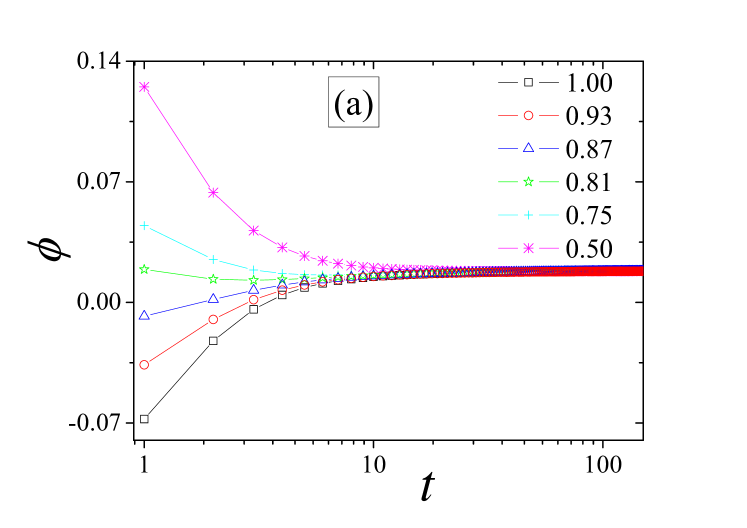
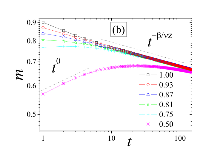
Figure 1: (a): Time evolution of the entropy flux $\phi$ obtained by MC simulations for different initial magnetizations $m_{0}$ indicated. (b) Time evolution of magnetization $m$ for different initial magnetizations $m_{0}$ indicated, obtained in the same simulations.

Figure 1b shows the typical short-time behavior expected for a spin model via MC simulations according to Eq. (11). Alternatively and only for a comparison, we can observe that some differences can be observed in mean-field regime by using the equations obtained in the previous section.

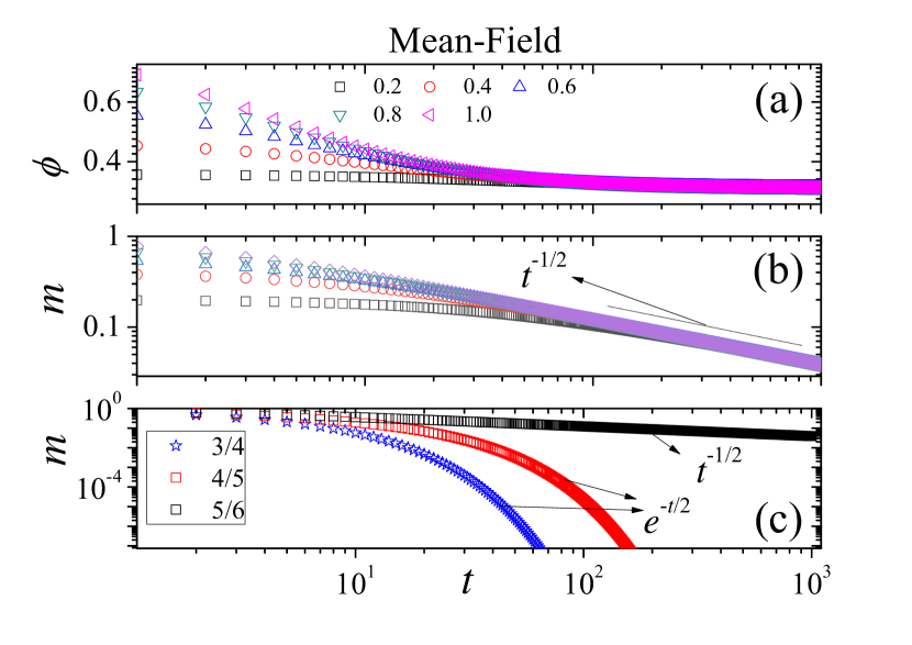
Figure 2: Simple mean-field analysis of the system. (a): Time evolution of the entropy flux $\phi$ for different initial magnetizations $m_{0}$ indicated at criticality $p_{c}=5/6$. (b) The corresponding time evolution of the magnetization $m$ also at criticality. (c) Deviation from $p=p_{c}$ of the magnetization $m$ for several values of $p$ indicated. The initial condition is $m_{0}=1$.

First, Fig. 2(a) shows that the mean-field entropy flux $\phi$ according to Eq. 21 independently of $m_{0}$ always decreases to reach the $\phi_{\infty}=(5/24)\ln 5\approx 0.33$ which is much bigger than the steady state value obtained for MC simulations. Differently from the MC simulations, in Fig. 2(b) we do not observe a initial slip for magnetization and we observe that $m(t)$ universally decays as $t^{-1/2}$. We believe that  absence of initial slip in mean-field short-time behavior must affect the differences on $\phi(t)$ via MC simulations and the MF approach. Finally, we plot the stretched exponential deviation from this power law considering $p<p_{c}$, which is also expected in STD theory when studied by time-dependent simulations, but we observe a more salient effect on the MF regime.

It is also interesting to investigate the power law verified in mean-field by Eq. (22). In this case we can study the quantity $\phi-\phi_{\infty}$ as function of $t$, expecting a power law behavior $\phi-\phi_{\infty}\sim t^{-\xi}$. Differently from mean-field regime, in MC simulations we expect $\xi_{MC}\neq\xi_{MF}=1$. In Fig. 3 we present a study of the quantity $\phi-\phi_{\infty}$ for two different situations: Fig. 3a with simulations starting from ferromagnetic inital state: $m_{0}=1$ and, Fig. 3b considering an disordered initial state with a very small initial magnetization, $m_{0}=1/2^{9}$. A stable power law can be observed up to $t_{\max}\approx 110\$MCsteps, and we obtained respectively $\xi=1.36(2)$ and $\xi=1.38(2)$ for $m_{0}=1$, and $m_{0}=1/2^{9}$ showing that there is no numerical evidence about a dependence on the initial condition of the system. We can observe that $\xi_{MC}>\xi_{MF}$, but in both cases the power law behavior is verified. Fig. 3c shows for a comparison, the time evolution of $\phi-\phi_{\infty}$ via mean field approximation calculated by substituting the result from the Eq: 17 in the Eq. 20. For $p=p_{c}=5/6$ we can observe a power law behavior (Eq. 21) and an exponential deviation can be observed for $p\ \neq p_{c}$.

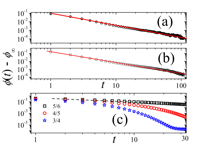
Figure 3: Power law behavior of the quantity $\phi-\phi_{\infty}$ obtained MC simulations: (a) $m_{0}=1$, and (b) $m_{0}=1/2^{9}$, and (c) the evolution of the same quantity obtained via mean-field for different values of $p$: $p=p_{c}=5/6$, $p=4/5$, and $p=3/4$.

Thus, we explore the MC simulations for $\alpha>0$. First we used a technique to localize and refine the critical parameters by considering a refinement method proposed in 2012 by two of the authors of this paper silva2012 . This approach, which is based on the refinement of the coefficient of determination of the order parameter, allows to locate phase transitions of systems in a very simple way.

Considering that discarding a certain $N_{\min}$ MC steps is needed since the universal behavior which we are looking for emerges only after a time period sufficiently long to avoid the microscopic short-time behavior (see for example some papers in several different models: with defined Hamiltonian shorttime and without defined Hamiltonian shorttime2 ). We can define the coefficient of determination as in silva2012 (see Appendix, section V)

$$r=\frac{\sum\limits_{t=N_{\min}}^{N_{MC}}(\overline{\ln m}-a-b\ln t)^{2}}{\sum\limits_{t=N_{\min}}^{N_{MC}}(\overline{\ln m}-\ln m(t))^{2}},$$ (23)

where $N_{MC}$ is the total number of MC steps and generically

$$\overline{O}=\frac{1}{(N_{MC}-N_{\min}+1)}\sum\nolimits_{t=N_{\min}}^{N_{MC}}O(t)\text{.}$$

The value of $N_{min}$ depends on the details of the system in study and it is related to the microscopic time scale, i.e., the time the system needs to reach the universal behavior in short-time critical dynamics janssen1989 .

When the system is near the criticality ($p\approx p_{c}$), for $m_{0}=1$, we expect that the order parameter follows a power law behavior $\overline{m(t)}\sim t^{-\beta/\nu z}\$which, in $\log\times\log$ scale, yields a linear behavior and $r$ approaches 1. In this case, we expect the slope $b$ to be a good estimate of $\beta/\nu z$. On the other hand, when the system is out of criticality, there is no power law and $r\simeq 0$. Thus, we are able to use the coefficient of determination $r$ to look for critical points. Thus, the idea of the method is very simple: we just need to sweep the parameter $p$ and find the point that possess $r\simeq 1$.

Thus, we performed simulations determining $p_{c}$ for each studied $\alpha$ studied (see Fig. 4), i.e., the best power corresponding to $\overline{m(t)}\sim t^{-\frac{\beta}{\nu z}}$ which occurs for ferromagnetic initial states, for example the case $\alpha=0$ can be observed in Fig. 1 (b).

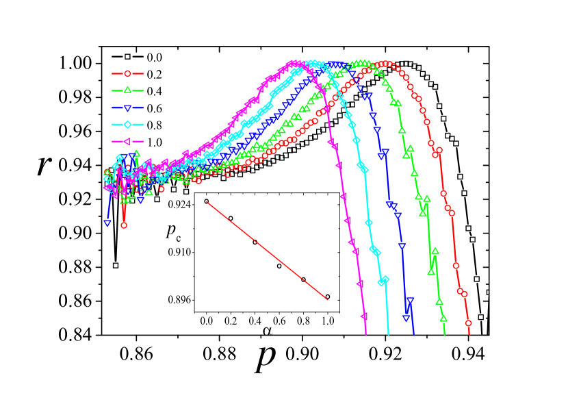
Figure 4: Determination coefficient $r$ as function of $p$ for different values of $\alpha$ indicated. The peak of these curves (maximum coefficient of determination correspond to the best $p_{c}$ obtained.

The inset plot in Fig. 4 shows the linear dependence of $p_{c}$ as function of $\alpha$. We use a resolution of $\Delta p=10^{-3}$. Thus, with these $p_{c}$ values in hands, we also determine $\theta=\theta(\alpha)$. For this task instead of studying the time evolution of magnetization for small values of $m_{0}$, and thus performing an extrapolation, we use the correlation of magnetization which also presents a power law with this specific exponent TomeOliveira1998 :

$$C(t)=\left\langle m(t)m(0)\right\rangle\sim t^{\theta},$$ (24)

where in this case, $\left\langle m(0)\right\rangle\approx 0$. We can observe in Fig. 5 the power law from our MC simulations for different mobility rates. In order to obtain the uncertainties on the exponent $\theta$ we repeat the same simulations for $N_{b}=5$ different beans, as well as the same procedure was used to obtain $\frac{\beta}{\nu z}$ by using the relaxation of ferromagnetic initial states.

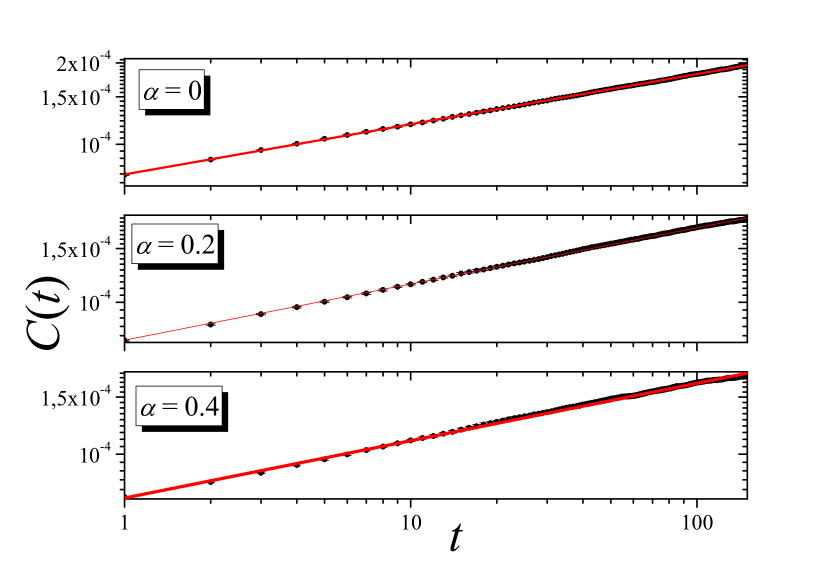
Figure 5: Power law behavior of the correlation given by Eq. 24 for three different diffusion levels.

In table 1 we show the value of exponents $\theta$ and $\beta/(\nu z)$ (last two columns) corresponding to different values of diffusion $\alpha$. We also show the values of critical parameters obtained by repeating the same optimization process for $N_{b}=5$ different seeds. We can observe that uncertainties leads to $\sigma_{p}=O(10^{-4})$ which is better than resolution of optimization procedure ($\Delta=10^{-3}$).

$\alpha$	$p_{c}(1)$	$p_{c}(2)$	$p_{c}(3)$	$p_{c}(4)$	$p_{c}(5)$	$\beta/(\nu z)$	$\theta$
0.0	0.925	0.925	0.925	0.924	0.925	0.0541(13)	0.185(6)
0.2	0.920	0.920	0.920	0.920	0.919	0.0642(15)	0.176(6)
0.4	0.913	0.914	0.913	0.913	0.913	0.0779(17)	0.160(2)
0.6	0.906	0.907	0.907	0.907	0.906	0.0932(36)	0.151(6)
0.8	0.902	0.902	0.902	0.902	0.902	0.0996(10)	0.14(1)
1.0	0.897	0.897	0.898	0.897	0.898	0.1108(29)	0.12(1)

Table 1: Critical parameters for 5 different repetitions of optimization and the corresponding exponents for each value of diffusion rate

We can observe that $\beta/(\nu z)$ increases while $\theta$ decreases as the diffusion rate increases, showing that diffusion has a important role in the phase transition of the model as observed for example in epidemic models and surface reaction models (see for example dasilva2018-2015 ). Just for a comparison of the exponents with other results only for $\alpha=0$, which is the only available estimates. In JFFMendes , the authors obtained $\theta=0.191(2)$ for MVM making extrapolation $m_{0}\rightarrow 0$ which in good agreement with our value. Both results also are in good agreement with results for the Ising model obtained by Grassberger Grassberger since both models are in the same universality class. It is also important to mention that our result is close to the value of $\beta/(\nu z)=0.0579(5)$, obtained by B. Zheng for the Ising model (see for example first reference in shorttime , pag. 1448).

By exploring some alternative results, we study the correlation of the entropy flux $C_{F}(t)=\left\langle\phi(t)\phi(0)\right\rangle$ for different diffusion rates. The results (see Fig. 6) show that correlation decay less quickly as the diffusion increases.

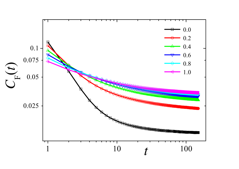
Figure 6: Decay of the correlation of the entropy flux as function of time for several values of $\alpha$ indicated.

Since we have explored the time-dependent results, we finally explore the effects of the diffusion on the entropy production which is equal to flux in the steady state. Here we call attention of the readers that we look for $p$ and not $q$ as the authors in Crochik2005 studied. We can look that our results for $\alpha=0$ recover that ones obtained by the authors (see Fig. 7 (a)) but, naturally, inverted.

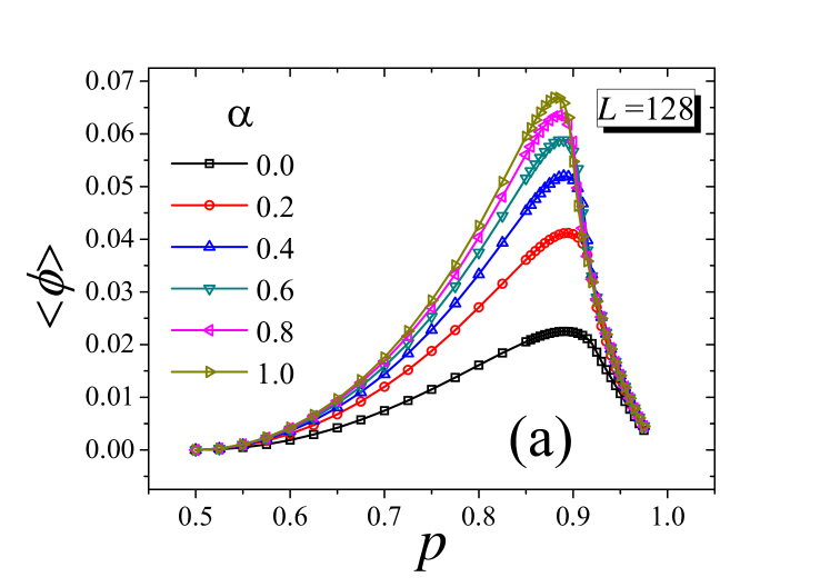
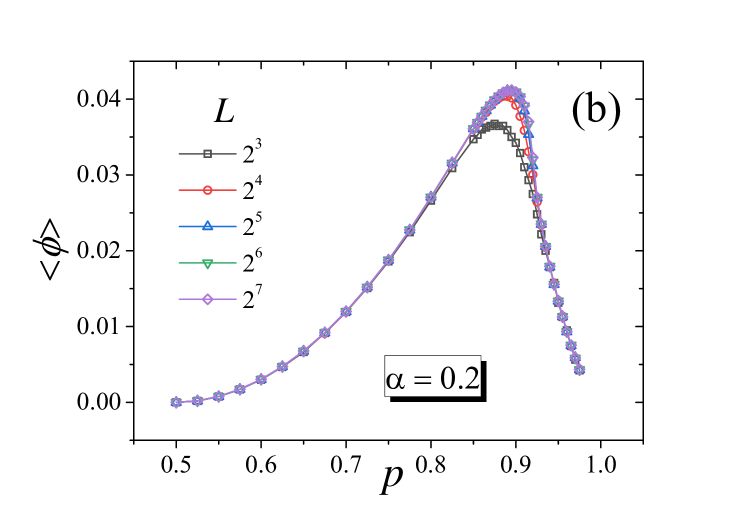
Figure 7: (a) Entropy production of entropy calculated via flux at steady state for different mobility rates for $L=128$. (b) Finite size effects tested for a specific value of mobility: $\alpha=0.2$. For $L\geq 32$ we do not observe differences between the plots.

This plot shows that entropy production (calculated as flux at steady state) increases as the diffusion enlarges. Fig 7 (b) shows that for $L\geq 32$ we have no observed differences in the plots of entropy production.

IV Summary and Conclusions

We have studied the diffusion effects on the Majority voter model exploring time-dependent and time independent properties of the entropy flux. Our results show that curve of entropy production enlarges as the diffusion rate enlarge for any value of $p$. We also studied the effects of the diffusion on the critical parameters of the model by using refinement procedure of power laws in short time. Our results show that critical parameter depends linearly on mobility rate. Similarly the dynamic exponents also depend on mobility rate. Mean-field results are revisited and we make a empirical comparison between short-time power law and entropy flux which still is a preliminary study and deserves future investigation in other models.

V Appendix

The coefficient of determination is a very simple concept used in linear fits, or other fits. Thus, let us briefly explain such standard procedure in the context of short-time MC simulations. When we perform least-square linear fit to a given data set, we obtain a linear predictor $\widehat{y}_{t}=a+bx_{t}$. In addition, if we consider the unexplained variation given by $\widetilde{\Delta}=\sum_{t=1}^{N}(y_{t}-\widehat{y}_{t})^{2}$ , and a perfect fit is achieved when the curve is given by $y_{t}=a+bx_{t}$, and therefore, $\widetilde{\Delta}=0$.

On the other hand, the explained variation $\Delta$ is given by the difference between the average $\overline{y}=N^{-1}\sum_{t=1}^{N}y_{t}$, and the prediction $\widehat{y}_{t}$, i.e., $\Delta=\sum_{t=1}^{N}(\widehat{y}_{t}-\overline{y})^{2}$. So, it is interesting to consider the total variation, naturally defined as $\Delta_{total}=\sum_{t=1}^{N}(y_{t}-\overline{y})^{2}$. So, we can rewrite this last expression as $\Delta_{total}=\sum_{t=1}^{N}(y_{t}-\widehat{y}_{t})^{2}+\sum_{t=1}^{N}(\widehat{y}_{t}-\overline{y})^{2}+\xi$, where $\xi=2\sum_{t=1}^{N}(y_{t}-\widehat{y}_{t})(\widehat{y}_{t}-\overline{y})$. However we can easily show that $\xi=0$, since

$$\begin{array}[]{lll}\sum_{t=1}^{N}(y_{t}-c_{a}-c_{b}x_{t})(c_{a}+c_{b}x_{t}-\overline{y})&=&c_{b}\sum_{t=1}^{N}x_{t}(y_{t}-c_{a}-c_{b}x_{t})\\ &&+\ (c_{a}-\overline{y})\sum_{t=1}^{N}x_{t}(y_{t}-c_{a}-c_{b}x_{t})\\ &&\\ &=&-\ \frac{c_{b}}{2}\frac{\partial}{\partial c_{b}}\sum_{t=1}^{N}(y_{t}-c_{a}-c_{b}x_{t})^{2}\\ &&-\ \frac{(c_{a}-\overline{y})}{2}\frac{\partial}{\partial c_{a}}\sum_{t=1}^{N}(y_{t}-c_{a}-c_{b}x_{t}),\end{array}$$ (25)

and the last two sums vanish by definition when take the least squares values $(c_{a},c_{b})=(a,b)$. Therefore, the total variation can be simply defined as

$$\Delta_{total}=\widetilde{\Delta}+\Delta\ ,$$ (26)

and the better the fit, the smaller the $\widetilde{\Delta}$. So, in an ideal situation $\widetilde{\Delta}=0$, and thus the ratio

$$r=\frac{\Delta}{\Delta_{total}}=1\ ,$$ (27)

i.e., the variation comes only from the explained sources.

So adapting this method to time-dependent MC simulations, if we consider that $y_{t}=\ln m(t+N_{\min})$, $x_{t}=\ln(t+N_{\min})$, where $N_{\min}$ is the number of MC steps discarded at the beginning of the simulation (the first steps), we can obtain the Eq. 23.

References

- (1) T. Tomé and M. J. Oliveira, Stochastic Dynamics and Irreversibility, Springer, Cham, 2015.
- (2) T. Tomé, M. J. de Oliveira, Phys. Rev. E 91, 042140 (2015).
- (3) N. G. van Kampen, Stochastic processes in physics and chemistry, North Holland, 1981.
- (4) L. Crochik, T. Tomé, Phys. Rev. E 72, 057103 (2005).
- (5) H. K. Janssen, B. Schaub, and B. Schmittmann, Z. Phys. B: Condens. Matter 73, 539 (1989).
- (6) H. Hinrichsen, Adv. Phys. 49, 815 (2000).
- (7) J. F. F. Mendes, M. A. Santos, Phys. Rev. E 57, 108 (1998)
- (8) M. J. de Oliveira, J. Stat. Phys. 66, 273 (1991)
- (9) G. Grinstein, , C. Jayaprakash, Y. He, Phys. Rev. Lett. 55, 2527 (1985)
- (10) C. Castellano, S. Fortunato, V. Loreto, Rev. Mod. Phys. 81, 591 (2009)
- (11) R. da Silva, J. R. Drugowich de Felício, and A. S. Martinez, Phys. Rev. E 85, 066707 (2012).
- (12) B. Zheng, Int. J. Mod. Phys. B, 12, 1419 (1998), E. V. Albano, M. A. Bab, G. Baglietto, R. A. Borzi, T. S. Grigera, E. S. Loscar, D. E. Rodriguez, M. L .R. Puzzo, G. P. Saracco, Rep. Prog. Phys. 74, 026501 (2011), R. da Silva, N. A. Alves and J. R. Drugowich de Felício, Phys. Rev. E 66, 026130 (2002)
- (13) T. Tomé, J.R. Drugowich de Felício, Modern Physics Letters B, 12, 873 (1998), T. Tomé, Braz. J. Phys., 30, 152-156 (2000), R. da Silva, N. Alves. Jr, Physica A, 350, 263 (2005).
- (14) T. Tomé, M. J. de Oliveira, Phys. Rev. E 58, 4242 (1998)
- (15) R. da Silva, H.A. Fernandes, Comp. Phys. Comm. 230, 1 (2018); J. Stat. Mech.: Theor. Exp., P06011 (2015)
- (16) P. Grassberger, Physica A 214, 547 (1995)