On the iterative solution of systems of the form $A^{\top}Ax=A^{\top}b+c$

Abstract

Given a full column rank matrix $A\in\mathbb{R}^{m\times n}$ ($m\geq n$), we consider a special class of linear systems of the form $A^{\top}Ax=A^{\top}b+c$ with $x,c\in\mathbb{R}^{n}$ and $b\in\mathbb{R}^{m}$. The occurrence of $c$ in the right-hand side of the equation prevents the direct application of standard methods for least squares problems. Hence, we investigate alternative solution methods that, as in the case of normal equations, take advantage of the peculiar structure of the system to avoid unstable computations, such as forming $A^{\top}A$ explicitly. We propose two iterative methods that are based on specific reformulations of the problem and we provide explicit closed formulas for the structured condition number related to each problem. These formula allow us to compute a more accurate estimate of the forward error than the standard one used for generic linear systems, that does not take into account the structure of the perturbations. The relevance of our estimates is shown on a set of synthetic test problems. Numerical experiments highlight both the increased robustness and accuracy of the proposed methods compared to the standard conjugate gradient method. It is also found that the new methods can compare to standard direct methods in terms of solution accuracy.

15A06, 65F10, 65F35, 65G50.

1 Introduction

Given $A\in\mathbb{R}^{m\times n}$, $m\geq n$ with $\mathrm{rank}(A)=n$, $b\in\mathbb{R}^{m}$ and $x,c\in\mathbb{R}^{n}$, we consider the following linear system of equations:

(1) $$A^{\top}Ax=A^{\top}b+c,$$

or, equivalently, the following minimization problem:

(2) $$\min_{x\in\mathbb{R}^{n}}\frac{1}{2}\|Ax-b\|^{2}-c^{\top}x.$$

At first sight, relation Eq. 1 evokes a least squares problem in the normal equations form:

(3) $$A^{\top}Ax=A^{\top}b,$$

but the situation is fundamentally different, as the vector $c$ is present in the right-hand side. Contrarily to least squares problems, a very well-studied topic ([3][16, Ch.5][23, Ch.10]), problem Eq. 1 has not been object of much study in the literature. It can be seen as a reformulation of a particular instance of a KKT system [8, 11, 15, 26]:

(4) $$\begin{bmatrix}H&A\\ A^{\top}&0\end{bmatrix}\begin{bmatrix}r\\ x\end{bmatrix}=\begin{bmatrix}b\\ -c\end{bmatrix}$$

where $H\in\mathbb{R}^{m\times m}$ is a symmetric matrix, in our case $H$ is the identity matrix. We mention [2] where the author studies the numerical solution of this augmented system by Gaussian elimination and a proper scaling.

The solution of problem Eq. 1 is however required in various applications in optimization, such as multilevel Levenberg-Marquardt methods [6], or in certain formulations based on penalty function approaches [13, 12, §7.2], that we describe in Section 2. Motivated by the important applications these problems arise from, we believe that it is worth getting more insights on both theoretical and practical aspects of the solution of Eq. 1, in particular on its solution by iterative methods.

Due to the similarity with the normal equations, we expect to encounter, both in the theoretical study of Eq. 1 and in the numerical solution, issues similar to those reported in the literature on normal equations.

First of all, the system matrix is the same. It is well known that the product $A^{\top}A$ should not be explicitly formed, because the accuracy attainable by methods for the solution of the normal equations may be much lower than that attainable by a backward stable method for least squares. In this case indeed, the best forward error bound for the normal equations can be obtained by the classical sensitivity analysis of linear systems. It is then of the order of $\kappa^{2}(A)~{}u$, with $u$ the machine precision and $\kappa(A)=\|A\|\|A^{\dagger}\|$ the condition number of $A$ in the Euclidean norm [19, 25]. This is an underwhelming result, as from Wedin’s theorem ([19, Theorem 20.1]) the sensitivity of a least squares problem is measured by $\kappa^{2}(A)$ only when the residual is large, and it is measured by $\kappa(A)$ otherwise.

However, practical solution methods do not form the product $A^{\top}A$, and the following key observation is rather exploited. The peculiar structure of the normal equations allows to write:

$$A^{\top}Ax-A^{\top}b=A^{\top}(Ax-b),$$

that makes it possible to either employ a factorization of $A$ rather than of $A^{\top}A$ (in the case of direct methods) or to perform matrix-vector multiplications of the form $A^{\top}x$ and $Ax$ rather than $A^{\top}Ax$ (in the case of iterative methods). This fact makes the standard conditioning analysis of linear systems unsuitable to predict the error for such methods, as the linear system is not subject to normwise perturbations on the matrix $A^{\top}A$, but rather to structured perturbations, such as perturbations in the matrix $A$ only. A structured conditioning analysis is then more relevant and indeed leads to the same conclusions as for least squares problems [17].

It is therefore possible to devise stable implementations of methods for normal equations. This has been deeply investigated in the literature, see, e.g., [4, 16, 24]. In [4] the specialized implementation of the Conjugate Gradient (CG) method for the normal equations (CGLS) has been proposed and shown to be more stable than CG applied directly to Eq. 3.

In general, however, not all the considerations made for normal equations directly apply to Eq. 1, since the right-hand side in Eq. 1 is $A^{\top}b+c$ instead of $A^{\top}b$. This difference has important consequences both on theoretical and practical sides.

On one hand, this results in a different mapping for the condition number and a different set of admissible perturbations for the backward error, as [14]. Consequently, the existing perturbation theory for least squares problems [1, 17, 27] does not apply here. A proper analysis of the structured condition number of the problem should then be developed.

From a practical perspective, even though the system matrix is the same, a fundamental difference appears: $A$ cannot be directly factorized on the right-hand side and standard methods for the normal equations cannot be directly applied. Successful algorithmic procedures used for normal equations could however be adapted to design stable solution methods, tailored for the specific problem that we consider.

Contributions

Inspired by the existing results on least squares problems, we propose two different reformulations of Eq. 1, such that it is possible to factorize the matrix $A$ on both the left and right-hand sides, and two corresponding solution methods. We provide structured condition numbers for Eq. 1 and for the proposed reformulations. These allow us to compute first order estimates of the forward error on the solution computed by the proposed methods. We also report on the numerical performance of such methods on a relevant set of test problems, considering also direct methods to provide a fair comparison. Extensive numerical experiments confirm an improved stability of the proposed methods compared to CG. The estimates of the forward error are also validated numerically and shown to be sharper upper bounds than the standard bounds issued from the theory of linear systems.

Structure

The manuscript is organized as follows. In Section 2 we present two applications arising in optimization where the solution of Eq. 1 is required. In Section 3, we report on the conditioning of the problem and backward error analysis. In Section 4, we discuss issues related to the solution of system of the form Eq. 1 in finite arithmetic. We remind specific algorithmic procedures successful for least squares problems (case $c=0$) that we later adapt to design stable methods for the solution of Eq. 1 (more general case $c\neq 0$). Then, we introduce and study the new iterative solution methods in Section 5. In Section 6 we propose first order estimates of the forward error on the solution computed by the proposed methods. Extensive numerical experiments are proposed in Section 7. Conclusions are drawn in Section 8.

Notation

Given a matrix $A\in\mathbb{R}^{m\times n}$, we denote by $A^{\dagger}$ its pseudoinverse, by $\kappa(A)=\|A\|\|A^{\dagger}\|$ the condition number of $A$ ($\|\cdot\|$ being the Euclidean norm) and by $\sigma_{\min}(A),\sigma_{\max}(A)$ the smallest and largest singular values of $A$, respectively. The Frobenius norm of $A$ is defined as

$$\|A\|_{F}:=\left(\sum_{i,j}\lvert A_{i,j}\rvert^{2}\right)^{1/2}=tr(A^{\top}A)^{1/2}.$$

Moreover, given $b\in\mathbb{R}^{m},c\in\mathbb{R}^{n}$, we define $\|[A,b,c]\|_{F}:=\sqrt{\|A\|_{F}^{2}+\|b\|^{2}+\|c\|^{2}}$. We later denote by $I_{n}\in\mathbb{R}^{n\times n}$ the identity matrix of order $n$, $\otimes$ the Kronecker product of two matrices and by $\mathrm{vec}$ the operator that stacks the columns of a matrix into a vector of appropriate dimension [17]. Given $\mathcal{X}$ and $\mathcal{Y}$ two normed subspaces equipped with norms $\|\cdot\|_{\mathcal{X}}$ and $\|\cdot\|_{\mathcal{Y}}$, respectively, we denote by $\|\cdot\|_{\mathrm{op}}$ the operator norm induced by the choice of $\|\cdot\|_{\mathcal{X}}$ and $\|\cdot\|_{\mathcal{Y}}$. Finally, given $a\in\mathbb{R}$, we denote by $\mathrm{fl}(a)$ its floating point representation, i.e. $\mathrm{fl}(a)$ is such that $\lvert a-\mathrm{fl}(a)\rvert\leq\lvert a\rvert\,u$, where $u$ represents the machine precision.

2 Two motivating applications

In this section, we describe two different applications in which problems of the form Eq. 2 arise, motivating our interest in their solution.

2.1 Fletcher’s exact penalty function approach

The first applicative context arises in equality constrained minimization. Consider a problem of the form:

$$\min_{x}f(x)$$

$$\text{ s.t. }g(x)=0,$$

for twice differentiable functions $f:\mathbb{R}^{n}\rightarrow\mathbb{R}$ and $g:\mathbb{R}^{n}\rightarrow\mathbb{R}^{m}$, respectively. The solution of systems of the form Eq. 1 is needed for the evaluation of the value and gradient of the following penalty function [13, 12, §7.2]:

$$\Phi_{\sigma}(x)=f(x)-g(x)^{\top}y_{\sigma}(x),$$

where $y_{\sigma}(x)\in\mathbb{R}^{m}$ is defined as the solution of the following minimization problem:

$$\min_{y}\|A(x)^{\top}y-\nabla f(x)\|^{2}+\sigma g(x)^{\top}y,$$

with $A(x)$ the Jacobian matrix of $g(x)$ at $x$ and $\sigma>0$, a given real-valued penalty parameter.

2.2 Multilevel Levenberg-Marquardt method

The second scenario, in which the solution of system Eq. 1 is required, arises in the setting of multilevel Levenberg-Marquardt methods, which are specific members of the family of multilevel optimization methods recently introduced in Calandra et al [6] and further analysed in Calandra et al [5]. The multilevel Levenberg-Marquardt method is intended to solve nonlinear least squares problems of the form:

$$\min_{x}f(x)=\frac{1}{2}\|F(x)\|^{2},$$

with $F:\mathbb{R}^{n}\rightarrow\mathbb{R}^{m}$, a twice continuously differentiable function. In the two-level setting, the multilevel method allows to choose between two different models to compute the step at each iteration: the classical Taylor model or a cheaper model $m_{k}^{H}$, built starting from a given approximation $f^{H}(x^{H})=\frac{1}{2}\|F^{H}(x^{H})\|^{2}$ to the objective function:

$$m_{k}^{H}(x_{k}^{H},s^{H})=\frac{1}{2}\|J^{H}(x_{k}^{H})s^{H}+F^{H}(x_{k}^{H})\|^{2}+\frac{\lambda_{k}}{2}\|s^{H}\|^{2}+(R\nabla f(x_{k})-\nabla f^{H}(x_{0}^{H}))^{\top}s^{H},$$

with $J^{H}(x_{k}^{H})$ the Jacobian matrix of $F^{H}$ at $x_{k}^{H}$, $\lambda_{k}>0$ a real-valued regularization parameter, $R$ a full-rank linear restriction operator and $x_{0}^{H}=Rx_{k}$, $x_{k}$ denoting the current iterate at fine level.

While minimizing the Taylor model amounts to solve a formulation based on the normal equations, minimizing $m_{k}^{H}$ requires the solution of a problem of the form Eq. 2, due to the addition of the correction term $(R\nabla f(x_{k})-\nabla f^{H}(x_{0}^{H}))^{\top}s^{H}$, that is needed to ensure coherence between levels. Approximate minimization of the model is sufficient to guarantee convergence of the method. Thus if the dimension of the coarse problem is not small, an iterative method is then particularly well suited for the minimization of the model.

3 Conditioning of the problem and backward error analysis

In this section we first study the conditioning of the problem Eq. 1. We first propose an explicit formula for the structured condition number, that is useful to compute a first order estimate of the forward error. We also propose theoretical results related to the backward error.

3.1 Conditioning of the problem

We study the conditioning of problem Eq. 1, i.e. the sensitivity of the solution $x$ to perturbations in the data $A,b,c$. We give an explicit formula for the structured condition number, for perturbations on all $A$, $b$ and $c$. In the following, we define the condition number of a function, see [25].

Definition 3.1.

If $F$ is a continuously differentiable function

$$F:\, \mathcal{X}\rightarrow\mathcal{Y}$$

$$x \longmapsto F(x),$$

the absolute condition number of $F$ at $x$ is the scalar $\|F^{\prime}(x)\|_{\mathrm{op}}$. The relative condition number of $F$ at $x$ is

$$\frac{\|F^{\prime}(x)\|_{\mathrm{op}}\,\|x\|_{\mathcal{X}}}{\|F(x)\|_{\mathcal{Y}}}.$$

We consider $F$ as the function that maps $A,b,c$ to the solution $x$ of Eq. 1:

$$F:\, \mathbb{R}^{m\times n}\times\mathbb{R}^{m}\times\mathbb{R}^{n}\rightarrow\mathbb{R}^{n}$$

$$(A,b,c)\longmapsto F(A,b,c)=A^{\dagger}b+A^{\dagger}(A^{\dagger})^{\top}c.$$

Let us define the true residual $r=b-Ax$. As in [17], we choose the Euclidean norm for the solution and the Frobenius norm (defined in the Notation part of Section 1) for the data.

In this section we mark perturbed quantities by a tilde. Let the $m\times n$ matrix $A$ be perturbed to $\tilde{A}=A+\delta A$, the $m$-dimensional vector $b$ to $\tilde{b}=b+\delta b$, the $n$-dimensional vector $c$ to $\tilde{c}=c+\delta c$. $A^{\top}A$ is then perturbed to

(5) $$\tilde{A}^{\top}\tilde{A}=(A+\delta A)^{\top}(A+\delta A)=A^{\top}A+\delta(A^{\top}A),\quad\delta(A^{\top}A)=A^{\top}\delta A+(\delta A)^{\top}A,$$

neglecting the second order terms. The solution $x=(A^{\top}A)^{-1}(A^{\top}b+c)$ is then perturbed to $\tilde{x}=x+\delta x=(\tilde{A}^{\top}\tilde{A})^{-1}(\tilde{A}^{\top}\tilde{b}+\tilde{c})$. Then, $\tilde{x}$ solves:

$$(A^{\top}A+\delta(A^{\top}A))\tilde{x}=(A^{\top}b+(\delta A)^{\top}b+A^{\top}\delta b+c+\delta c).$$

Reminding Eq. 5, and that, since $A$ is full column rank, $A^{\dagger}=(A^{\top}A)^{-1}A^{\top}$ and $(A^{\top}A)^{-1}=A^{\dagger}(A^{\dagger})^{\top}$, we have

$$\delta x=(A^{\top}A)^{-1}(\delta A)^{\top}r-A^{\dagger}\delta Ax+A^{\dagger}\delta b+A^{\dagger}(A^{\dagger})^{\top}\delta c.$$

From this, we conclude that

$$F^{\prime}(A,b,c)(E,f,g)=(A^{\top}A)^{-1}E^{\top}r-A^{\dagger}Ex+A^{\dagger}f+A^{\dagger}(A^{\dagger})^{\top}g,$$

for all $E\in\mathbb{R}^{m\times n},f\in\mathbb{R}^{m},g\in\mathbb{R}^{n}$. We then deduce the following property:

Lemma 3.2.

The conditioning of the problem Eq. 1, with Euclidean norm on the solution and Frobenius norm on the data, is given by

(6) $$\|F^{\prime}(A,b,c)\|_{\mathrm{op}}=\|[(r^{\top}\otimes(A^{T}A)^{-1})L_{T}+x^{\top}\otimes A^{\dagger},A^{\dagger},(A^{T}A)^{-1}]\|,$$

where $L_{T}$ is the linear operator such that $\mathrm{vec}(A^{\top})=L_{T}\mathrm{vec}(A)$ ($L_{T}$ is a permutation matrix consisting of ones in the positions $(n(k-1)+l,m(l-1)+k)$ with $l=1,\dots,n$ and $k=1,\dots,m$ and of zeros elsewhere [14, 17]).

In the following, we give an explicit and computable formula for the structured condition number.

Theorem 3.3.

The absolute condition number of problem Eq. 1, with Euclidean norm on the solution and Frobenius norm on the data, is $\sqrt{\rule[0.0pt]{0.0pt}{8.9626pt}\|\bar{M}\|}$, with $\bar{M}\in\mathbb{R}^{n\times n}$ given by

(7) $$\bar{M}=(1+\|r\|^{2})(A^{\top}A)^{-2}+(1+\|x\|^{2})(A^{\top}A)^{-1}-2~{}\mathrm{sym}(B),$$

with $B=A^{\dagger}rx^{\top}(A^{T}A)^{-1}$, $\mathrm{sym}(B)=\frac{1}{2}(B+B^{\top})$ and $x$ the exact solution of Eq. 1.

Proof 3.4.

Let us define $M=[(r^{\top}\otimes(A^{T}A)^{-1})L_{T}+x^{\top}\otimes A^{\dagger},A^{\dagger},(A^{T}A)^{-1}]$. We remind that

(8) $$\|F^{\prime}(A,b,c)\|_{\mathrm{op}}=\|M\|=\|M^{\top}\|:=\sup_{y\neq 0}\frac{\|M^{\top}y\|}{\|y\|}.$$

Let us consider

$$y^{\top}F^{\prime}(A,b,c)(E,f,g) =y^{\top}(A^{\top}A)^{-1}E^{\top}r-y^{\top}A^{\dagger}Ex+y^{\top}A^{\dagger}f+y^{\top}A^{\dagger}(A^{\dagger})^{T}g$$

$$=r^{\top}E(A^{T}A)^{-1}y-y^{\top}A^{\dagger}Ex+y^{\top}A^{\dagger}f+y^{\top}A^{\dagger}(A^{\dagger})^{T}g.$$

We remind that $E=\sum_{i=1}^{n}\sum_{j=1}^{m}e_{i}^{\top}Ee_{j}$, for $e_{i},e_{j}$ the $i$-th and $j$-th vectors of the canonical basis. Then, we can rewrite the expression as

$$[\mathrm{vec}(S),y^{\top}A^{\dagger},y^{\top}A^{\dagger}(A^{\dagger})^{T}]\cdot[\mathrm{vec}(E),f,g]^{\top}:=w^{\top}[\mathrm{vec}(E),f,g]^{\top},$$

introducing the matrix $S$ such that:

$$S_{i,j}=r^{\top}e_{i}e_{j}^{\top}(A^{T}A)^{-1}y-y^{\top}A^{\dagger}e_{i}e_{j}^{\top}x.$$

It follows that $w=M^{\top}y$. We are then interested in the norm of $w$. We can compute the squared norm of $\mathrm{vec}(S)$ as:

$$\|\mathrm{vec}(S)\|^{2} = \sum_{i=1}^{n}\sum_{j=1}^{m}(r^{\top}e_{i}e_{j}^{\top}(A^{T}A)^{-1}y-y^{\top}A^{\dagger}e_{i}e_{j}^{\top}x)^{2}$$

$$= \|r\|^{2}\|(A^{T}A)^{-1}y\|^{2}+\|x\|^{2}\|(A^{\dagger})^{\top}y\|^{2}$$

$$-y^{\top}(A^{\dagger}rx^{\top}(A^{T}A)^{-1}+(A^{T}A)^{-1}xr^{\top}(A^{\dagger})^{\top})y.$$

Then,

$$\|w\|^{2}= ~{}y^{\top}((1+\|r\|^{2})(A^{\top}A)^{-2}+(1+\|x\|^{2})A^{\dagger}(A^{\dagger})^{\top}-(A^{\dagger}rx^{\top}(A^{T}A)^{-1}$$

$$+(A^{T}A)^{-1}xr^{\top}(A^{\dagger})^{\top})y:=y^{\top}\bar{M}y.$$

From Eq. 8

$$\|F^{\prime}(A,b,c)\|_{\mathrm{op}}=\|M\|=\sup_{y\neq 0}\frac{\|M^{\top}y\|}{\|y\|}=\sup_{y\neq 0}\frac{\sqrt{y^{\top}\bar{M}y}}{\|y\|}=\sqrt{\rule[0.0pt]{0.0pt}{8.9626pt}\|\bar{M}\|},$$

and we obtain the thesis.

We remark here a fundamental difference with the least squares case. In the conditioning of least squares or structured conditioning of the normal equations, the term $\kappa^{2}(A)$ appears multiplied by the norm of the residual. This is interpreted saying that the sensitivity of the problem depends on $\kappa(A)$ for small or zero residual problems and on $\kappa^{2}(A)$ for all other problems [3, 19]. In this case, we notice from Eq. 7 that a term proportional to $\kappa^{2}(A)$ will always be present.

3.2 Backward error analysis

In this section, we address the computation of the backward error, i.e. we consider the following problem. Let $A\in\mathbb{R}^{m\times n}$, $b\in\mathbb{R}^{m}$, $c\in\mathbb{R}^{n}$ and $\tilde{x}$ a perturbed solution to Eq. 1. Find the smallest perturbation $(E,f,g)$ of $(A,b,c)$ such that the vector $\tilde{x}$ exactly solves

$$(A+E)^{\top}(A+E)x=(A+E)^{\top}(b+f)+(c+g),$$

i.e. given

$$\mathcal{G}:=\{(E,f,g) ,E\in\mathbb{R}^{m\times n},f\in\mathbb{R}^{m},g\in\mathbb{R}^{n}\,:$$

$$(A+E)^{\top}(A+E)\tilde{x}=(A+E)^{\top}(b+f)+(c+g)\},$$

we want to compute the quantity:

(9) $$\eta(\tilde{x},\theta_{1},\theta_{2})=\min_{(E,f,g)\in\mathcal{G}}\|[E,\theta_{1}f,\theta_{2}g]\|_{F}^{2}:=\min_{(E,f,g)\in\mathcal{G}}\|E\|_{F}^{2}+\theta_{1}^{2}\|f\|^{2}+\theta_{2}^{2}\|g\|^{2},$$

with $\theta_{1},\theta_{2}$ positive parameters. As usually done in the literature on backward errors, see, for example, [17, 27], we measure the perturbations in a weighted Frobenius norm.

We prove specific results related to the backward error. We provide an explicit representation of the set of admissible perturbations on the matrix (Theorem 3.5) and a linearization estimate for $\eta(\tilde{x},\theta_{1},\theta_{2})$ (Lemma 3.7), respectively.

Given $v\in\mathbb{R}^{m}$, we define

$$v^{\dagger}=\begin{cases}\displaystyle\frac{v^{\top}}{\|v\|^{2}}\quad&\text{ if }v\neq 0,\\ 0\quad&\text{ if }v=0.\end{cases}$$

We remind the following properties that will be used later:

$$(I_{m}-vv^{\dagger})v=0, vv^{\dagger}v=v.$$

We consider just perturbations on the matrix and we give next an explicit representation of the set of admissible perturbations.

Theorem 3.5.

Let $A\in\mathbb{R}^{m\times n}$, $b\in\mathbb{R}^{m}$, $c,\tilde{x}\in\mathbb{R}^{n}$ and assume that $\tilde{x}\neq 0$. Let $\tilde{r}=b-A\tilde{x}$ and define two sets $\mathcal{E,M}$ by

$$\mathcal{E}= \{E\in\mathbb{R}^{m\times n}:\;(A+E)^{\top}(b-(A+E)\tilde{x})=-c\,\},$$

$$\mathcal{M}= \{v\left(\alpha c^{\top}-v^{\dagger}A\right)+(I_{m}-vv^{\dagger})(\tilde{r}\tilde{x}^{\dagger}+Z(I_{n}-\tilde{x}\tilde{x}^{\dagger}))\;:$$

$$v\in\mathbb{R}^{m},\,Z\in\mathbb{R}^{m\times n},\alpha\in\mathbb{R},\,s.t.\,\,\alpha\|v\|^{2}(v^{\dagger}b-\alpha c^{\top}\tilde{x})=-1\}.$$

Then $\mathcal{E}=\mathcal{M}$.

Proof 3.6.

The proof is inspired by that of [27, Theorem 1.1]. First, we prove $\mathcal{E}\subseteq\mathcal{M}$. Let $E\in\mathcal{E}$, then $E$ can be written as

(10) $$E=(I_{m}-vv^{\dagger})E\tilde{x}\tilde{x}^{\dagger}+vv^{\dagger}E+(I_{m}-vv^{\dagger})E(I_{n}-\tilde{x}\tilde{x}^{\dagger}).$$

We choose $v=\tilde{r}-E\tilde{x}$. Then $E\tilde{x}=\tilde{r}-v$ and

(11) $$(I_{m}-vv^{\dagger})E\tilde{x}=(I_{m}-vv^{\dagger})\tilde{r}.$$

Moreover, it holds

(12) $$-c=(A+E)^{\top}(b-(A+E)\tilde{x})=(A+E)^{\top}(\tilde{r}-E\tilde{x})=(A+E)^{\top}v.$$

From Eq. 12, $v^{\dagger}E=-\displaystyle\frac{c^{\top}}{\|v\|^{2}}-v^{\dagger}A$. Hence, from relations Eq. 10, Eq. 11 and Eq. 12

$$E=(I_{m}-vv^{\dagger})\tilde{r}\tilde{x}^{\dagger}-v\left(\frac{c^{\top}}{\|v\|^{2}}+v^{\dagger}A\right)+(I_{m}-vv^{\dagger})E(I_{n}-\tilde{x}\tilde{x}^{\dagger}).$$

Then $E\in\mathcal{M}$ with $v=\tilde{r}-E\tilde{x}$, $\alpha=-\displaystyle\frac{1}{\|v\|^{2}}$ and $Z=E$, as

$$\alpha\|v\|^{2}(v^{\dagger}b-\alpha c^{\top}\tilde{x}) =-\frac{1}{\|v\|^{2}}(v^{\top}b+c^{\top}\tilde{x})=-\frac{1}{\|v\|^{2}}(v^{\top}b-v^{\top}(A+E)\tilde{x})$$

$$=-\frac{1}{\|v\|^{2}}v^{\top}(\tilde{r}-E\tilde{x})=-1,$$

where the second equality follows from Eq. 12.

Conversely, let $E\in\mathcal{M}$. Then,

(13) $$E\tilde{x} =\alpha vc^{\top}\tilde{x}-vv^{\dagger}A\tilde{x}+\tilde{r}-vv^{\dagger}\tilde{r}=\alpha vc^{\top}\tilde{x}-vv^{\dagger}b+\tilde{r},$$

(14) $$E^{\top}v =\alpha\|v\|^{2}c-A^{\top}v.$$

Then,

$$(A+E)^{\top}(b-(A+E)\tilde{x}) =(A+E)^{\top}(\tilde{r}-E\tilde{x})=(A+E)^{\top}(vv^{\dagger}b-\alpha vc^{\top}\tilde{x})$$

$$=(A+E)^{\top}v(v^{\dagger}b-\alpha c^{\top}\tilde{x})=\alpha\|v\|^{2}c(v^{\dagger}b-\alpha c^{\top}\tilde{x})=-c,$$

where the second equality follows from Eq. 13, the fourth one from Eq. 14 and the last one from the constraint in $\mathcal{M}$. From this we conclude that $E\in\mathcal{E}$, which completes the proof.

Let us remark that if $c=0$ we recover the known result for least squares problems given in [27, Theorem 1.1]. We also note that the parametrization of the set of perturbations $\mathcal{E}$ is similar to that obtained for equality constrained least squares problems in [9], where the constraint is however not present.

Due to the constraint in $\mathcal{M}$, it is rather difficult to find an analytical formula for $\eta(\tilde{x},\theta_{1},\theta_{2})$. It is however easy to find a linearization estimate for $\eta(\tilde{x},\theta_{1},\theta_{2})$ with $\theta_{1},\theta_{2}$ stricly positive, i.e., given

$$h(A,b,c,x)=A^{\top}(b-Ax)+c,$$

to find $(E,f,g)$ such that

(15a) $$\bar{\eta}(\tilde{x},\theta_{1},\theta_{2}) =\min\|[E,\theta_{1}f,\theta_{2}g]\|_{F}\quad\text{s.t.}$$

(15b) $$h(A,b,c,\tilde{x}) +[J_{A},\theta_{1}^{-1}J_{b},\theta_{2}^{-1}J_{c}]\begin{bmatrix}\mathrm{vec}(E)\\ \theta_{1}f\\ \theta_{2}g\end{bmatrix}=0,$$

where $J_{A}$, $J_{b}$ and $J_{c}$ are the Jacobian matrices of $h$ with respect to $\mathrm{vec}(A)$, $b$, $c$ [7].

Lemma 3.7.

Let ${\eta}(\tilde{x},\theta_{1},\theta_{2})$ be defined as in Eq. 9, $\bar{\eta}(\tilde{x},\theta_{1},\theta_{2})$ be defined as in Eq. 15 and $\tilde{r}=b-A\tilde{x}$. Then

$$\bar{\eta}(\tilde{x},\theta_{1},\theta_{2})=\Bigg{\|}\begin{bmatrix}vec(E)\\ \theta_{1}f\\ \theta_{2}g\end{bmatrix}\Bigg{\|}=\|J^{\dagger}h(A,b,c,\tilde{x})\|,$$

with

$$J:=[I_{n}\otimes\tilde{r}^{\top}-A^{\top}(\tilde{x}\otimes I_{m}),\theta_{1}^{-1}A^{\top},\theta_{2}^{-1}I_{n}].$$

Moreover, assume that $\tilde{r}\neq 0$. If $4\eta_{1}\|J^{\dagger}\|\eta(\tilde{x},\theta_{1},\theta_{2})\leq 1$, then

$$\frac{2}{1+\sqrt{2}}~{}\bar{\eta}(\tilde{x},\theta_{1},\theta_{2})\leq\eta(\tilde{x},\theta_{1},\theta_{2})\leq 2~{}\bar{\eta}(\tilde{x},\theta_{1},\theta_{2}),$$

where $\eta_{1}=\sqrt{\theta_{1}^{-2}+\theta_{2}^{-2}+\|\tilde{x}\|^{2}}$.

Proof 3.8.

The first assertion follows as a simple modification of the results in Section 2 of [22]. Simply adding the term corresponding to $c$ in the linearization leads to:

$$[J_{A},\theta_{1}^{-1}J_{b},\theta_{2}^{-1}J_{c}]=[I_{n}\otimes\tilde{r}^{\top}-A^{\top}(\tilde{x}\otimes I_{m}),\theta_{1}^{-1}A^{\top},\theta_{2}^{-1}I_{n}]=J,$$

from which the result follows. The second result can be obtained repeating the arguments of [22, Corollary 2].

The linearized estimate is usually called an asymptotic estimate, as it becomes exact in the limit for $\tilde{x}$ that tends to the exact solution $x$ [22]. It also has the advantage of being easily computable.

In this section we have considered theoretical questions related to the solution of Eq. 1. In the following, we will consider the approximation of a solution in finite arithmetic.

4 Finite arithmetic implementation of CG for $A^{\top}Ax=A^{\top}b+c$

In this section, we address the implementation of CG in finite arithmetic. We first discuss the well-known case $c=0$, that corresponds to the normal equations for least squares problems. In particular, we briefly remind the issues arising in finite precision when applying CG to such systems, and the successful algorithmic ingredients that make CGLS more stable than CG. We then consider the more general case $c\neq 0$ and show that the same issues also arise in this case. These observations are found crucial for the development of stable solution methods for Eq. 1. In Section 5 indeed, the successful ingredients employed in the case $c=0$ will be extended to the more general case $c\neq 0$.

4.1 Case $c=0$

In [4] the authors study the implementation of CG applied to the normal equations in finite arithmetic and, thanks to a rounding error analysis, individuate the operations which may lead to amplifications of initial errors in the data, and so to large perturbations in the solution. Then, they propose the CGLS method, which is a more stable implementation of CG for normal equations. For convenience, we report both algorithms, in Algorithm 1 and Algorithm 2, respectively.

Two different sources of numerical error do occur when applying CG on the normal equations. First, computing $\mathrm{fl}(A^{\top}A)$ can lead to a loss of information. CGLS avoids forming matrix $A^{\top}A$ explicitly. Matrix-vector products are thus computed exploiting subsequently the action of $A$ and of its transpose on a vector, whereas the computation of $p_{k}^{\top}A^{\top}Ap_{k}$ is performed as $\|Ap_{k}\|^{2}$. The second source of error comes from the right-hand side $b$. Assuming that $x_{0}=0$, the only information related to $b$ is in the initialization of $p_{1}=A^{\top}(b-Ax_{0})$, see Algorithm 1. No further reference to $b$ is made in the iterative procedure. It then follows that roundoff errors that occur in computing the vector $A^{\top}b$ cannot be compensated for later [4]. Hence, in CGLS, the residual of the normal equations $r_{k}=A^{\top}(b-Ax_{k})$ is not recurred directly. Rather, $d_{k}=b-Ax_{k}$ is recurred, while $r_{k}$ is then updated multiplying $d_{k}$ by $A^{\top}$. The next result is also proved, which is an extension of the corresponding result in [18], where the author studies the finite precision implementation of the class of iterative methods considered in Lemma 4.1.

Lemma 4.1.

Let $A\in\mathbb{R}^{m\times n}$. Consider an iterative method in which each step updates the approximate solution $x_{k}$ and the residual $r_{k}$ of the system $Ax=b$ using the two formulas:

$$x_{k+1} =x_{k}+\alpha_{k}~{}p_{k},$$

$$r_{k+1} =r_{k}-\alpha_{k}~{}Ap_{k},$$

with $\alpha_{k}\in\mathbb{R}$, $p_{k}\in\mathbb{R}^{n}$ and $x\in\mathbb{R}^{n}$ the true solution. The difference between the true residual $b-Ax_{k}$ and the recursively computed residual $r_{k}$ satisfies

(16) $$\frac{\|b-Ax_{k}-r_{k}\|}{\|A\|\|x\|}\leq u~{}O(k)\left(1+\Theta_{k}+\frac{\|r\|}{\|A\|\|x\|}\right),$$

with $u$ the machine precision, $r=b-Ax$ and $\Theta_{k}=\max_{j\leq k}\|x_{j}\|/\|x\|$.

Lemma 4.1 is used in [4] to deduce a bound on the forward error for such methods:

(17) $$\frac{\|x-x_{k}\|}{\|x\|}\leq\kappa(A)~{}u~{}O(k)\left(3+\frac{\|r\|}{\|A\|\|x\|}\right)+\kappa(A)\frac{\|r-r_{k}\|}{\|A\|\|x\|}.$$

It is shown in [4, 18] that the residuals $r_{k}$ generated by CG tend towards zero, so that $x_{k}$ will eventually remain unchanged. In the bound $k$ can therefore be replaced by $S$, the number of iterations necessary to reach this steady-state. Then, if

(18) $$\frac{\|r-r_{S}\|}{\|A\|\|x\|}\leq c_{1}u$$

for a strictly positive constant $c_{1}$, we deduce that the method may compute more accurate solutions than a backward stable method [4].

4.2 Case $c\neq 0$

When using CG applied to Eq. 1, observations similar to those made in the previous section can be made. If the right-hand side $A^{\top}b+c$ is formed, an error occurs. We can indeed quantify this error as in [4], §4. Following [4], we assume the following model of floating point arithmetic on a machine with roundoff $u$:

$$\mathrm{fl}(a\,\mathrm{op}\,b)=(a\,\mathrm{op}\,b)(1+\delta(ab)),\quad\lvert\delta(ab)\rvert\leq u,\quad\mathrm{op}\in\{+,-,\times,\div\}$$

This leads to a bound for the roundoff error in the product of two matrices $A\in\mathbb{R}^{m\times n}$ and $B\in\mathbb{R}^{n\times p}$:

(19) $$\lvert\mathrm{fl}(AB)-AB\rvert\leq\gamma_{n}\lvert A\rvert\lvert B\rvert,\qquad\gamma_{n}=nu/(1-nu),$$

where the inequalities are to be interpreted componentwise [4, 19]. It is assumed that $nu\ll 1$.

Errors are introduced when the product $A^{\top}b$ and the sum with $c$ in the right-hand side are performed. The perturbed solution $\tilde{x}=x+\delta x$ corresponding to the system with perturbed right-hand side $\mathrm{fl}(\mathrm{fl}(A^{\top}b)+c)$ will satisfy, assuming that the linear systems are solved exactly:

(20) $$A^{\top}A\tilde{x}=\mathrm{fl}(\mathrm{fl}(A^{\top}b)+c).$$

From relation Eq. 19 we obtain

(21) $$\mathrm{fl}(A^{\top}b) =A^{\top}b+\delta_{1},\quad\quad\lvert\delta_{1}\rvert\leq\gamma_{m}\lvert A^{\top}\rvert\lvert b\rvert,$$

(22) $$\mathrm{fl}(\mathrm{fl}(A^{\top}b)+c) =A^{\top}b+c+\delta_{1}+\delta_{2},\quad\lvert\delta_{2}\rvert\leq u\lvert A^{\top}b+c\rvert+O(u^{2}).$$

Subtracting Eq. 1 from Eq. 20 and solving for $\delta x$, we obtain from Eq. 21-Eq. 22:

$$\lvert\delta x\rvert\leq \lvert(A^{\top}A)^{-1}\rvert\lvert\delta_{1}+\delta_{2}\rvert\leq\gamma_{m}\lvert(A^{\top}A)^{-1}\rvert\lvert A^{\top}\rvert\lvert b\rvert+u\lvert(A^{\top}A)^{-1}\rvert\lvert A^{\top}b+c\rvert$$

(23) $$\leq \gamma_{m+1}\lvert(A^{\top}A)^{-1}\rvert\lvert A^{\top}\rvert\lvert b\rvert+u\lvert(A^{\top}A)^{-1}\rvert\lvert c\rvert$$

From the singular value decomposition of $A$, it is possible to deduce the following relations, see [3] §1.4.3:

$$\|(A^{\top}A)^{-1}\|=\frac{1}{\sigma_{\min(A)}^{2}},\,\|A\|=\sigma_{\max}(A),\,\|A^{\dagger}\|=\frac{1}{\sigma_{\min(A)}}.$$

Exploiting these relations and extending inequality Eq. 23 to the norm, we obtain:

$$\|\delta x\|\leq \gamma_{m+1}\|(A^{\top}A)^{-1}\|\|A^{\top}\|\|b\|+u\|(A^{\top}A)^{-1}\|\|c\|,$$

$$\leq \gamma_{m+1}\kappa(A)\|A^{\dagger}\|\|b\|+u\|A^{\dagger}\|^{2}\|c\|,$$

(24) $$\leq u\kappa^{2}(A)\left(\frac{m+1}{1-(m+1)u}\frac{\|b\|}{\|A\|}+\frac{\|c\|}{\|A\|^{2}}\right).$$

Since $b$ and $c$ are not used in the iterative process, this initial error will not be cancelled and the best forward error bound we can hope for will include the term given above, which may be larger than the error introduced by the solution of the linear system, as we will see in Section 7. Then, if this initial rounding error is larger than the optimal bound $\sqrt{\rule[0.0pt]{0.0pt}{8.9626pt}\|\bar{M}\|}\|[A,b,c]\|_{F}u$ we can expect CG to produce less than optimal solutions. This will happen for example if

$$\|b\|\|A\|+\|c\|>>\left[1+\|r\|+2\sqrt{\|c\|\|x\|}+\frac{1+\|x\|}{\|A^{\dagger}\|}\right]\sqrt{\|A\|_{F}^{2}+\|b\|^{2}+\|c\|^{2}},$$

where the second term has been obtained from an upper bound to the condition number $\sqrt{\rule[0.0pt]{0.0pt}{8.9626pt}\|\bar{M}\|}$.

Similarly, the residual of the perturbed solution may differ from the true residual by as much as

$$\|A^{\top}b+c-(A^{\top}A)(x+\delta x)-(A^{\top}b+c-A^{\top}Ax)\|=$$

$$=\|A^{\top}A\delta x\|\leq\gamma_{m+1}\kappa(A)^{2}\|A\|\|b\|+u\kappa(A)^{2}\|c\|,$$

and again, this cannot be cancelled in the iterations.

Algorithm 1 Conjugate Gradient for $Ax=b$ (CG)

  Input: $A$, $b$, $x_{0}$.

  Define $r_{0}=b-Ax_{0}$, $p_{1}=r_{0}$.

  for  $k=1,2,\dots$  do

     $\alpha_{k}=\displaystyle\frac{r_{k-1}^{\top}r_{k-1}}{p_{k}^{\top}Ap_{k}}$,

     $x_{k}=x_{k-1}+\alpha_{k}p_{k}$,

     $r_{k}=r_{k-1}-\alpha_{k}Ap_{k}$,

     $\beta_{k}=\displaystyle\frac{r_{k}^{\top}r_{k}}{r_{k-1}^{\top}r_{k-1}}$,

     $p_{k+1}=r_{k}+\beta_{k}p_{k}$.

  end for

Algorithm 2 Conjugate Gradient Least Squares for $A^{\top}Ax=A^{\top}b$ (CGLS)

   Input: $A$, $b$, $x_{0}$.

  Define $d_{0}=b-Ax_{0}$, $r_{0}=A^{\top}d_{0}$, $p_{1}=r_{0}$.

  for  $k=1,2,\dots$  do

     $t_{k}=Ap_{k}$,

      $\alpha_{k}=\displaystyle\frac{r_{k-1}^{\top}r_{k-1}}{t_{k}^{\top}t_{k}}$,

      $x_{k}=x_{k-1}+\alpha_{k}p_{k}$,

     $d_{k}=d_{k-1}-\alpha_{k}t_{k}$,

     $r_{k}=A^{\top}d_{k}$,

     $\beta_{k}=\displaystyle\frac{r_{k}^{\top}r_{k}}{r_{k-1}^{\top}r_{k-1}}$,

     $p_{k+1}=r_{k}+\beta_{k}p_{k}$.

  end for

Thus, when solving system Eq. 1, we encounter the same problems as with the normal equations. Our aim is then to exploit the particular structure of Eq. 1, that is close to that of normal equations, to extend the successful algorithmic ingredients used in that case to design stable methods in our specific setting.

5 Proposed iterative solution methods

In this section, we introduce two solution methods for Eq. 1. They exploit specific reformulations of the original problem or approximations to it, to be able to factorize $A$ on both the left- and the right-hand sides.

Having in mind the possibility of seeking an approximate solution, we especially focus on iterative methods, that are intended to be more stable than the standard CG method, later used as a reference method. We propose and describe the two methods, named CGLS$\epsilon$ and CGLS$I$, respectively. We first explain the ideas on which their designs are based and then present an extensive numerical evaluation in Section 7.

5.1 CGLS$\epsilon$

The first approach we propose is based on the solution of a least squares problem, with both matrix and right-hand side depending on an auxiliary real-valued strictly positive parameter $\epsilon$. The problem is defined in a way that its solution $x_{\epsilon}$ approximates the true solution of Eq. 1 $x$, when the parameter $\epsilon$ goes to zero. This reformulation is especially convenient because we can exploit the structure of the normal equations and solve the problem with CGLS, hence avoiding the issues described in Section 4.

Given $\epsilon>0$, let us then define

(25) $$A_{\epsilon}=\begin{bmatrix}A\\ \epsilon~{}c^{\top}\end{bmatrix},\quad b_{\epsilon}=\begin{bmatrix}b\\ \displaystyle 1/\epsilon\end{bmatrix}.$$

We then consider the following linear least squares problem:

(26) $$\min_{x}\|A_{\epsilon}x-b_{\epsilon}\|^{2}.$$

We remark that, due to the presence of $\epsilon$ in the right-hand side which is expected to be a small quantity, the residual will generally be really large. From standard perturbation theory on least squares problems, when the residual is large, the sensitivity of the system depends on $\kappa^{2}(A_{\epsilon})\|A_{\epsilon}x_{\epsilon}-b_{\epsilon}\|/(\|A_{\epsilon}\|\|x_{\epsilon}\|)$. Hence, problem Eq. 26 would then generally be severely ill-conditioned. However, the classical results are not so meaningful in this case, as the components of $b_{\epsilon}$ and $A_{\epsilon}$ have different magnitudes, see Remark 1.4.3 in Björck [3].

A more meaningful analysis is proposed next in Theorem 5.1, whose proof can be easily derived analogously to that of Theorem 3.3.

Theorem 5.1.

Let $F_{\epsilon}$ be the function that maps $A,b,c$ to the solution $x_{\epsilon}$ of Eq. 26:

$$F_{\epsilon}:\, \mathbb{R}^{m\times n}\times\mathbb{R}^{m}\times\mathbb{R}^{n}\rightarrow\mathbb{R}^{n}$$

$$(A,b,c)\longmapsto F_{\epsilon}(A,b,c)=(A_{\epsilon}^{\top}A_{\epsilon})^{-1}(A^{\top}b+c),$$

and let $r_{\epsilon}=b-Ax_{\epsilon}$. The absolute condition number of problem Eq. 26, with Euclidean norm on the solution and Frobenius norm on the data, is then given by:

$$\|F^{\prime}_{\epsilon}(A,b,c)\|_{\mathrm{op}}=\| [(r_{\epsilon}^{\top}\otimes(A_{\epsilon}^{\top}A_{\epsilon})^{-1})L_{T}+x_{\epsilon}^{\top}\otimes(A_{\epsilon}^{\top}A_{\epsilon})^{-1}A^{\top},$$

$$(A_{\epsilon}^{\top}A_{\epsilon})^{-1}A^{\top},(1-2\epsilon c^{\top}x_{\epsilon})(A_{\epsilon}^{\top}A_{\epsilon})^{-1}]\|,$$

where $L_{T}$ is the linear operator introduced in Lemma 3.2. This condition number can be equivalently expressed as $\sqrt{\rule[0.0pt]{0.0pt}{8.9626pt}\|\bar{M}_{\epsilon}\|}$, with

$$\bar{M}_{\epsilon}= ~{}((1-2\epsilon c^{\top}x_{\epsilon})^{2}+\|r_{\epsilon}\|^{2})(A_{\epsilon}^{\top}A_{\epsilon})^{-2}+(1+\|x_{\epsilon}\|^{2})(A_{\epsilon}^{\top}A_{\epsilon})^{-1}A^{\top}A(A_{\epsilon}^{\top}A_{\epsilon})^{-1}$$

(27) $$-2~{}\mathrm{sym}(B_{\epsilon})$$

with $B_{\epsilon}=(A_{\epsilon}^{\top}A_{\epsilon})^{-1}A^{\top}r_{\epsilon}x_{\epsilon}^{\top}(A_{\epsilon}^{\top}A_{\epsilon})^{-1}$ and $\mathrm{sym}(B_{\epsilon})=\frac{1}{2}(B_{\epsilon}+B_{\epsilon}^{\top})$.

It is essential to notice that from Theorem 5.1, the conditioning of Eq. 26 does not depend on $\|b_{\epsilon}-A_{\epsilon}x_{\epsilon}\|$, that will be really large, but rather on $\|r_{\epsilon}\|=\|b-Ax_{\epsilon}\|$, that will be indeed much smaller. The normal equations for Eq. 26 are

(28) $$(A^{\top}A+\epsilon^{2}cc^{\top})x=A^{\top}b+c,$$

that is, if $\epsilon$ goes to zero, the matrix of Eq. 28 is close to that of the normal equations Eq. 1. We can then prove that the solution of Eq. 28 approximates a solution of Eq. 1 for small $\epsilon$.

Lemma 5.2.

Let $x_{\epsilon}$ be the solution of Eq. 28 and $x$ be the solution of Eq. 1. Then, $\displaystyle{\lim_{\epsilon\rightarrow 0}x_{\epsilon}=x}$ and the relative norm of the error satisfies

(29) $$\frac{\|x_{\epsilon}-x\|}{\|x\|}\leq\epsilon^{2}\frac{\|c\|\|w\|}{1+\epsilon^{2}c^{\top}w},\quad w=(A^{\top}A)^{-1}c.$$

Proof 5.3.

$A^{\top}A+\epsilon^{2}cc^{\top}$ is obtained as a rank one correction of $A^{\top}A$. Thus the application of the Sherman-Morrison formula [3, §3.1.2] leads to:

$$x_{\epsilon}=x-\frac{\epsilon^{2}c^{\top}x}{1+\epsilon^{2}c^{\top}w}w,\quad w=(A^{\top}A)^{-1}c.$$

Then we obtain

$$\frac{\|x_{\epsilon}-x\|}{\|x\|}\leq\epsilon^{2}\frac{\|c\|\|w\|}{1+\epsilon^{2}c^{\top}w},$$

which completes the proof.

This result is helpful to propose a practical choice for $\epsilon$, that can be related to $\kappa(A)$. Note however that, to have guarantee of obtaining an accurate solution, a relatively small $\epsilon$ may be needed, depending on $\|w\|$. One may be then concerned that a really small $\epsilon$ may cause large errors in finite arithmetic, but we can show that an arbitrarily small value can indeed be used. A perturbed solution $\tilde{x}_{\epsilon}=x_{\epsilon}+\delta x_{\epsilon}$ will be such that:

$$(A_{\epsilon}^{\top}A_{\epsilon})(\delta x_{\epsilon})=\delta(A_{\epsilon}^{\top}b_{\epsilon}).$$

We need little care in evaluating $\delta(A_{\epsilon}^{\top}b_{\epsilon})$, as the standard bound

$$\lvert\delta(A_{\epsilon}^{\top}b_{\epsilon})\rvert\leq\gamma_{m+1}\lvert A_{\epsilon}^{\top}\lvert\rvert b_{\epsilon}\rvert$$

will largely overestimate it, due to the possibly large norm of $b_{\epsilon}$. Indeed, in practical computations, the large last component of $b_{\epsilon}$ is compensated by the multiplication with the small entries in the last line of $A_{\epsilon}$. We consider that

$$\mathrm{fl}(A_{\epsilon}^{\top}b_{\epsilon})=\mathrm{fl}(A^{\top}b)+\mathrm{fl}\left(\epsilon c\frac{1}{\epsilon}\right)+\delta_{s},$$

with $\delta_{s}$ an additional error due to the summation. We remark that if we assume $\epsilon$ to represent a machine number, i.e. $\epsilon=2^{i}$ for $i\in\mathbb{Z}$, then $\mathrm{fl}\left(\epsilon~{}c~{}\displaystyle\frac{1}{\epsilon}\right)=c$, the computation is performed exactly, as it just amounts of a shift in the exponent. Then,

$$\mathrm{fl}\left(A_{\epsilon}^{\top}b_{\epsilon}\right)=A^{\top}b+c+\delta_{p}+\delta_{s},\;\;\text{ with }\;\;\lvert\delta_{s}\rvert\leq u\lvert A^{\top}b+c\rvert+O(u^{2}),\;\lvert\delta_{p}\rvert\leq\gamma_{m}\lvert A\rvert\lvert b\rvert,$$

and the bound does not depend on $\epsilon$. The first approach we propose, called CGLS$\epsilon$, is based on the solution of Eq. 26 with the CGLS method. From Lemma 5.2, if we choose a small value for $\epsilon$, we can expect the computed solution to be an accurate approximation to $x$. We will later discuss the choice of this free parameter in Section 7.2.

5.2 CGLS$I$

The second method we propose is still based on the solution of an augmented system. In this case, we do not employ any auxiliary parameter. We rather use an auxiliary matrix $\hat{I}\in\mathbb{R}^{(m+1)\times(m+1)}$ and we define $\hat{A}\in\mathbb{R}^{(m+1)\times n}$ and $\hat{b}\in\mathbb{R}^{m+1}$, accordingly:

$$\hat{A}=\begin{bmatrix}A\\ c^{\top}\end{bmatrix},\qquad\hat{I}=\left[\begin{array}[]{cc}I_{m}&0\\ 0&0\\ \end{array}\right],\qquad\hat{b}=\begin{bmatrix}b\\ 1\end{bmatrix}.$$

We then reformulate Eq. 1 as:

$$\hat{A}^{\top}\hat{I}\hat{A}x=\hat{A}^{\top}\hat{b},$$

the two systems being equivalent. Although this reformulation is not a least squares problem, it still offers the advantage to factorize $\hat{A}^{\top}$ in both the right- and the left-hand sides. Hence, we can use a Krylov subspace method as a solution method, that can be implemented with no need of forming matrix $\hat{A}^{\top}\hat{I}\hat{A}$ explicitly or of recurring the residual $r=\hat{A}^{\top}(\hat{I}\hat{A}x-\hat{b})$. We can rather simply update $\hat{d}=\hat{I}\hat{A}x-\hat{b}$ along the iterations and form $r$ by multiplication with $\hat{A}^{\top}$. This allows to avoid corruption of $b$ by multiplication with $A^{\top}$ at the beginning of the process, without possibility of amending for it. We describe the whole procedure in Algorithm 3.

Algorithm 3 CGLS$I$ for $A^{\top}Ax=A^{\top}b+c$

   Input: $\hat{A}$, $\hat{b}$, $x_{0}$

  Define $\hat{d}_{0}=\hat{b}-\hat{A}x_{0}$, $r_{0}=\hat{A}^{\top}(\hat{b}-\hat{A}x_{0})$, $p_{1}=r_{0}$.

  for $k=1,2,\dots$ do

      $\hat{t}_{k}=\hat{I}\hat{A}p_{k}$,

      $\alpha_{k}=\displaystyle\frac{r_{k-1}^{\top}r_{k-1}}{\hat{t}_{k}^{\top}\hat{t}_{k}}$,

     $x_{k}=x_{k-1}+\alpha_{k}p_{k}$,

     $\hat{d}_{k}=\hat{d}_{k-1}-\alpha_{k}\hat{t}_{k}$,

     $r_{k}=\hat{A}^{\top}\hat{d}_{k}$,

     $\beta_{k}=\displaystyle\frac{r_{k}^{\top}r_{k}}{r_{k-1}^{\top}r_{k-1}}$,

     $p_{k+1}=r_{k}+\beta_{k}p_{k}$.

  end for

In exact arithmetic the method in Algorithm 3 is equivalent to CG applied to Eq. 1. The practical implementation of CGLS$I$ just relies on the use of augmented matrices together with two expedients to make the method more stable: the computation of $p_{k}^{\top}A^{\top}Ap_{k}$ as $\|\hat{I}\hat{A}p_{k}\|^{2}$ and the update of the residual. We can therefore expect the same benefits of CGLS as compared to CG.

Remark 5.4.

Lemma 4.1 also applies to the CGLS$I$ method with $A$ replaced with $\hat{I}\hat{A}$. We can then deduce that, if condition Eq. 18 holds, the bound Eq. 17 is also valid and CGLS$I$ will provide numerical solutions to Eq. 1 in a stable way. As pointed out in [4], proving condition Eq. 18 is not an easy task. Nevertheless, we have found that this condition is shown to be satisfied numerically after extensive numerical experimentations, see Section 7. We also point out that the condition number of $\hat{A}$ can be related to that of $A$ by [20, Corollary 7.3.6]. We finally notice that Lemma 4.1 also applies to CGLS$\epsilon$. Nevertheless it is not so meaningful, since in Eq. 16 the quantity $\|A_{\epsilon}x_{\epsilon}-b_{\epsilon}\|$ would be rather large.

6 First order approximation for the forward error

The formulas we have derived in Theorem 3.3 and Theorem 5.1 for the structured condition number of problems Eq. 1 and Eq. 26 can be used to provide a first order estimate of the forward error on a solution obtained by a method that does not form the matrix $A^{\top}A$ or $A_{\epsilon}^{\top}A_{\epsilon}$ explicitly. We define these estimates as the product of the relative condition number (see Definition 3.1) and the linearized estimate of the backward error in Lemma 3.7.

For CGLS$I$, we use the relative condition number

(30) $$\frac{\sqrt{\rule[0.0pt]{0.0pt}{8.9626pt}\|\bar{M}\|}\|[A,b,c]\|_{F}}{\|x\|}$$

of Eq. 1 for perturbations on $A$, $b$, $c$, with $\bar{M}$ defined in Eq. 7.

For CGLS$\epsilon$, the error on the computed solution $\hat{x}_{\epsilon}$ depends on two terms, the distance of the computed solution to the exact solution of Eq. 28 and the distance of the exact solution of Eq. 28 to the exact solution of Eq. 1:

(31) $$\frac{\|x-\hat{x}_{\epsilon}\|}{\|x\|}\leq\frac{\|x-x_{\epsilon}\|}{\|x\|}+\frac{\|x_{\epsilon}-\hat{x}_{\epsilon}\|}{\|x\|}=\frac{\|x-x_{\epsilon}\|}{\|x\|}+\frac{\|x_{\epsilon}-\hat{x}_{\epsilon}\|}{\|x_{\epsilon}\|}\frac{\|x_{\epsilon}\|}{\|x\|}.$$

The first term and the ratio $\displaystyle\frac{\|x_{\epsilon}\|}{\|x\|}$ can be bounded by the Sherman-Morrison formula, see Eq. 29, while the second one by using the relative condition number

(32) $$\frac{\sqrt{\rule[0.0pt]{0.0pt}{8.9626pt}\|\bar{M}_{\epsilon}\|}\|[A,b,c]\|_{F}}{\|x\|}$$

obtained in Theorem 5.1, with $\bar{M}_{\epsilon}$ defined in Theorem 5.1.

For CG, we can use the same bound as for CGLS$I$, adding the initial rounding error Eq. 24 due to the computation of the right-hand side.

Given the computed solution $\hat{x}$, we then define the following error estimates:

(33a) $$\hat{E}_{CGLSI}:=\frac{\sqrt{\rule[0.0pt]{0.0pt}{8.9626pt}\|\bar{M}\|}\|[A,b,c]\|_{F}}{\|\hat{x}\|}\bar{\eta}(\hat{x}),$$

(33b) $$\hat{E}_{CGLS_{\epsilon}}:=\epsilon^{2}\frac{\|c\|\|w\|}{1+\epsilon^{2}c^{\top}w}+\frac{\sqrt{\rule[0.0pt]{0.0pt}{8.9626pt}\|\bar{M}_{\epsilon}\|}\|[A,b,c]\|_{F}}{\|\hat{x}\|}\bar{\eta}_{\epsilon}(\hat{x}_{\epsilon})\Big{\|}I_{n}-\frac{\epsilon^{2}wc^{\top}}{1+\epsilon^{2}c^{\top}w}\Big{\|},$$

(33c) $$\hat{E}_{CG}:=\frac{\sqrt{\rule[0.0pt]{0.0pt}{8.9626pt}\|\bar{M}\|}\|[A,b,c]\|_{F}}{\|\hat{x}\|}\bar{\eta}(\hat{x})+\kappa^{2}(A)\bar{\eta}(\hat{x})\left(\frac{m+1}{1-(m+1)u}\frac{\|b\|}{\|A\|}+\frac{\|c\|}{\|A\|^{2}}\right),$$

$\bar{\eta}(\hat{x}),\bar{\eta}_{\epsilon}(\hat{x}_{\epsilon})$ being the linearized estimates of the backward error of the corresponding problem.

We will show in Section 7.3.2 that the proposed estimates nicely predict the actual error in the numerical simulations and that in all cases they provide upper bounds for the forward error.

7 Numerical experiments

We numerically validate the performance of the methods presented in Section 5. We discuss their practical implementation and evaluate the first order estimates of the forward error based on the relative condition numbers derived in Section 6. To provide a fair comparison, we also consider CG, MINRES (applied to Eq. 4) and standard direct methods. We show that CGLS$I$ and CGLS$\epsilon$ perform better than CG and that they can compare with direct methods, in terms of solution accuracy.

7.1 Problem definition and methodology

All the numerical methods have been implemented in Matlab. For CGLS$\epsilon$, CG and MINRES, Matlab codes available online have been employed. For CG, the computation $A^{\top}A$ is avoided and the products of $A^{\top}A$ times a vector are computed by successive multiplication by $A$ and its transpose. We consider linear systems of the form Eq. 1, where the matrix $A\in\mathbb{R}^{m\times n}$ has been obtained as $A=U\Sigma V^{\top}$, where $U$ and $V$ have been selected as orthogonal matrices generated with the Matlab commands gallery(’orthog’,m,j), gallery(’orthog’,n,j), respectively, for different choices of $j=1,\dots,6$. We consider two choices for the diagonal elements of $\Sigma$:

• : $\Sigma_{ii}=a^{-i}$, for $a>0$,

• : $\Sigma_{ii}=u_{i}$, where $u\in\mathbb{R}^{n}$ is generated with the linspace Matlab command i.e. $u=\sf{linspace}(\sf{dw,up},n)$, with $\sf{dw,up}$ being strictly positive real values,

for $i=1,\dots,n$.

The numerical tests are intended to show specific properties of the method. We therefore consider matrices of relatively small dimensions ($m=40$ and $n=20$), in order to avoid too ill-conditioned problems [4]. For all the performance profiles reported in the following, we consider a set of $40$ matrices of slightly larger dimension ($m=100$, $n=50$), that we later call $\mathcal{P}$, to also test the robustness of the methods (we however do not focus here with issues related to large scale problems). This set is composed of selected matrices from the gallery Matlab command (those with condition number still lower than $10^{10}$), and synthetic matrices corresponding to both choices C1 and C2 (of size $100\times 50$ rather than $40\times 20$). The condition number of the matrices is found to be between $1$ and $10^{10}$. The optimality measure considered is the relative solution accuracy $\displaystyle\frac{\|x-\hat{x}\|}{\|x\|}$, with $x$ the exact solution (chosen to be $x=[n-1,n-2,\dots,0]^{\top}$) and $\hat{x}$ the computed numerical solution (we omit the subscript $\epsilon$ for CGLS$\epsilon$). In the tests $c$ is freely chosen and $b=Ax-{A^{\dagger}}^{\top}c$. A simulation is considered unsuccessful if the relative solution accuracy is larger than $10^{-2}$.

We first focus on iterative methods. Before performing a detailed comparison, we address a practical question in CGLS$\epsilon$: how to choose the parameter $\epsilon$ ?

7.2 How to choose $\epsilon$ in CGLS$\epsilon$?

In this section we exclusively focus on CGLS$\epsilon$ and on the choice of parameter $\epsilon$.

In exact arithmetic, when $\epsilon$ goes to zero, applying CGLS to Eq. 28 is equivalent to applying CG to Eq. 1. However, in practice a fixed value for $\epsilon$ has to be chosen. This choice should minimize the error on the computed solution $\hat{x}_{\epsilon}$, which depends on two terms, the distance of the computed solution to the exact solution of Eq. 28 and the distance of the exact solution of Eq. 28 to the exact solution of Eq. 1, as it is shown in relation Eq. 31.

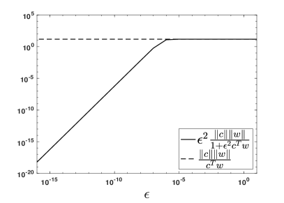
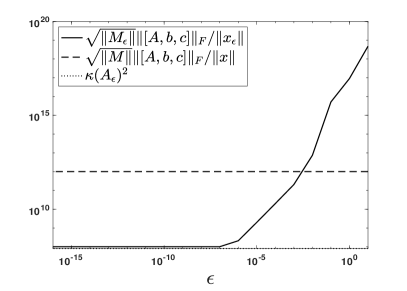
We plot the estimates of these two terms as a function of $\epsilon$ in Fig. 1, for the test corresponding to $c=\sf{rand}(n,1)$ and choice C2 with $\sf{dw}=10^{-7}$, $\sf{up}=0.1$. Specifically, on Fig. 1 left we plot the estimate Eq. 29 (solid line) of $\displaystyle\frac{\|x-x_{\epsilon}\|}{\|x\|}$ for different values of $\epsilon$ ($\epsilon=2^{-27}\approx 10^{-8},2^{-34}\approx 10^{-10},2^{-40}\approx 10^{-12},2^{-47}\approx 10^{-14},2^{-54}\approx 10^{-16}$). On Fig. 1 right we plot the relative condition number Eq. 32, solid line.

With decreasing $\epsilon$, the solution of Eq. 28 approximates increasingly better that of Eq. 1, and the relative condition number improves and converges to that of Eq. 1 in Eq. 30 (dotted line in the right part of Fig. 1). A small value of $\epsilon$ will then make both error terms small.

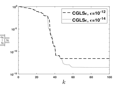
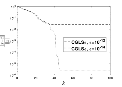
Special attention should however be paid when the norm of the right-hand side is large. Indeed, in this case the value of $\epsilon$ that is necessary to let the method converge to a solution of Eq. 1, may be really small. Let us explain why.

Let us assume to apply Algorithm 1 to Eq. 1 and Algorithm 2 to Eq. 28. We would respectively compute:

$$\alpha_{1}=\frac{\|r_{0}\|^{2}}{p_{1}^{\top}A^{\top}Ap_{1}}=\frac{\|A^{\top}b+c\|^{2}}{\|A(A^{\top}b+c)\|^{2}}, x_{1}=\alpha_{1}(A^{\top}b+c)=\alpha_{1}p_{1},$$

and

$$\alpha_{1}(\epsilon)=\frac{\|A^{\top}b+c\|^{2}}{\|A(A^{\top}b+c)\|^{2}+\epsilon\|c^{\top}(A^{\top}b+c)\|}, x_{1}(\epsilon)=\alpha_{1}(\epsilon)p_{1}(\epsilon)=\alpha_{1}(\epsilon)p_{1}.$$

Notice that if $\epsilon$ tends to zero, so does the term $\epsilon\|c^{\top}(A^{\top}b+c)\|$ in the denominator of $\alpha_{1}(\epsilon)$. Consequently $\alpha_{1}(\epsilon)$ tends toward $\alpha_{1}$ and $x_{1}(\epsilon)$ tends toward $x_{1}$. If $\epsilon$ has to be fixed, its value should be small enough to let $\epsilon\|c^{\top}(A^{\top}b+c)\|$ be small compared to $\|A(A^{\top}b+c)\|^{2}$, otherwise the found approximation will be close to a solution of Eq. 28 rather than to one of Eq. 1. This choice is then particularly difficult when $\|A^{\top}b+c\|$ is large.

We show this phenomenon on a test case reported in Fig. 2. We take choice C1 with $a=1.3$. It holds $\kappa(A)=10^{2}$. We first choose $c=10^{-2}\,\sf{rand}(n,1)$ (Fig. 2 left) and then $c=10^{2}\,\sf{rand}(n,1)$ (Fig. 2 right). We report the relative error ${\|x-\hat{x}\|}/{\|x\|}$ versus the number of iterations $k$. The related system has been solved by CGLS$\epsilon$, for two different values of $\epsilon\approx 10^{-12},10^{-14}$. We can remark that in both cases the lower value of the parameter allows for a lower relative error but especially in the second test the difference is really important. This is due to the fact that in the second test the norm of $c$ is much larger than in the first test, so that a smaller value of $\epsilon$ would be needed to let the term $\epsilon\|c^{\top}(A^{\top}b+c)\|$ be negligible with respect to $\|A(A^{\top}b+c)\|$.

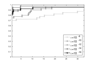
Finally, in Fig. 3, we report a performance profile [10], built on the set of matrices $\mathcal{P}$. The performance of the method improves as $\epsilon$ becomes smaller, both in terms of robustness and accuracy, with the best corresponding to $\epsilon\approx 10^{-14}$, as shown in Fig. 3. Lower values of $\epsilon$ do not improve the performance of the method.

Conclusion: A small value of $\epsilon$ is found to guarantee the best performance, and ensures CGLS$\epsilon$ to be less sensible to right-hand sides with large Euclidean norm. Then, later we choose $\epsilon=2^{-47}\approx 10^{-14}$.

Figure 1: CGLS$\epsilon$. Left part: Estimate Eq. 29 of $\|x_{\epsilon}-x\|/\|x\|$ for different values of $\epsilon$ (solid line) and limit value for $\epsilon\rightarrow\infty$ (dashed line), $w=(A^{\top}A)^{-1}c$. Right part: relative condition number Eq. 32 for different values of $\epsilon$ (solid line) and relative condition number for $\epsilon=0$, from Eq. 30 (dotted line). Notice that for small values of $\epsilon$ the structured condition number of the problem is far less than $\kappa(A_{\epsilon})^{2}$ (dashed line).

Figure 2: CGLS$\epsilon$. Relative error $\displaystyle\frac{\|x-\hat{x}\|}{\|x\|}$ between the exact solution $x$ and the computed solution $\hat{x}$ for $\epsilon\approx 10^{-12}$ (dashed line) and $\epsilon\approx 10^{-14}$ (dotted line) versus iteration index $k$. Left part: $c=10^{-2}\,\sf{rand(n,1)}$, right part: $c=10^{2}\,\sf{rand(n,1)}$.

Figure 3: CGLS$\epsilon$. Performance profile of CGLS$\epsilon$ on the synthetic set of matrices $\mathcal{P}$ for different values of $\epsilon$.

7.3 Comparing CGLS$\epsilon$ and CGLS$I$ with CG

In this section, we compare the performance of CGLS$\epsilon$ (with $\epsilon=2^{-47}\approx 10^{-14}$) and CGLS$I$ to the reference CG method. We first show their increased performance on selected problems.

7.3.1 Solution accuracy

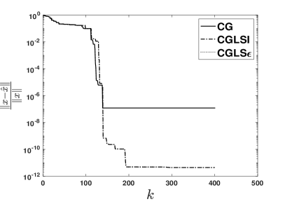
We first consider the numerical experiment corresponding to choice C1 with $a=0.5$ and we choose $c=10^{-1}\,\sf{rand}(n,1)$. The corresponding matrix $A$ is such that $\kappa(A)=10^{5}$. The three iterative methods are compared in Fig. 4 left, where we report the relative error ${\|x-\hat{x}\|}/{\|x\|}$ versus the number of iterations $k$. The practical behaviour of the methods is found to be different. CG achieves an accuracy of the order of $10^{-7}$, while the error in the solution computed by CGLS$I$ and CGLS$\epsilon$ is $\kappa(A)$ times lower.

Figure 4: Relative error $\displaystyle\frac{\|x-\hat{x}\|}{\|x\|}$ between the exact solution $x$ and the computed solution $\hat{x}$ for CG, CGLS$I$ and CGLS$\epsilon$, respectively. Left part: $\kappa(A)=10^{5}$. Right part: $\kappa(A)=5\,10^{7}.$

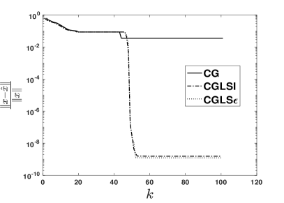
We now consider a second numerical experiment based on the choice C2 with $\sf{up}=0.5$, $\sf{dw}=10^{-8}$, $c=10^{-14}\,\sf{rand}(n,1)$ respectively. It holds $\kappa(A)=5\,10^{7}$. The gap in the results is even larger, both CGLS$I$ and CGLS$\epsilon$ find an accurate solution, while CG does not manage to solve the problem at all, see Fig. 4 right.

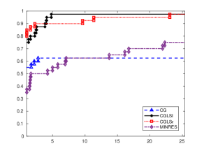
We finally compare the three iterative methods plus MINRES on the synthetic set of matrices $\mathcal{P}$, where $c$ is chosen as $\gamma+(\zeta-\gamma)\,\sf{rand}(n,1)$ for different values of $\gamma,\zeta$. We report in Fig. 5 the performance profile corresponding to these simulations. Clearly, CGLS$I$ and CGLS$\epsilon$ perform much better than CG and MINRES. Their performance is quite similar but CGLS$I$ is found more robust on problems with right-hand sides of large Euclidean norm. In addition, CGLS$I$ offers the advantage to be parameter free.

Figure 5: Performance profile of CG, CGLS$I$, CGLS$\epsilon$ and MINRES on the synthetic set of matrices $\mathcal{P}$.

7.3.2 Forward error bounds

In this section we numerically validate the error estimates Eq. 33.

In Table 1 we validate these bounds for different problems of the form C1 and C2. We report the condition number of matrix $A$, the bound on the forward error coming from standard theory of linear systems and, for each method, the forward error and the estimates from Eq. 33. For all the tests, the proposed first order estimates provide an accurate upper bound for the forward error and in many tests they are much sharper than the standard bound. It is again evident from these tests that in general CGLS$I$ and CGLS$\epsilon$ perform better than CG. In particular, in many tests the initial error introduced while forming the right-hand side, see Eq. 24, is larger than the error related to the solution of the linear system.

Notice also that using the standard results on least squares problems for CGLS$\epsilon$ would largely overestimate the error. For example, for the first test we would obtain:

$$\frac{\|\hat{x}_{\epsilon}-x_{\epsilon}\|}{\|x_{\epsilon}\|}\leq u~{}\kappa(A_{\epsilon})\left(1+\frac{\|A_{\epsilon}^{\dagger}\|\|b_{\epsilon}-A_{\epsilon}x_{\epsilon}\|}{\|x_{\epsilon}\|}\right)\approx 3\,10^{-8}.$$

This is evident also from Fig. 1 right, where we remark that $\kappa^{2}(A_{\epsilon})$ alone is already much larger than the structured relative condition number of Eq. 26.

Problem	$\kappa(A)$	$\kappa(A)^{2}\bar{\eta}(\hat{x})$	$E_{CG}$	$\hat{E}_{CG}$	$E_{CGLSI}$	$\hat{E}_{CGLSI}$	$E_{CGLS\epsilon}$	$\hat{E}_{CGLS\epsilon}$
$a=2$, $\alpha=10^{-10}$	$5\,10^{5}$	$6\,10^{-5}$	$6\,10^{-7}$	$10^{-5}$	$2\,10^{-10}$	$3\,10^{-6}$	$2\,10^{-10}$	$4\,10^{-7}$
$a=0.4$, $\alpha=10^{-12}$	$10^{7}$	$10^{-1}$	$10^{-3}$	$10^{-2}$	$10^{-8}$	$4\,10^{-8}$	$7\,10^{-11}$	$5\,10^{-8}$
$a=0.7$, $\alpha=10^{-1}$	$10^{3}$	$2\,10^{-10}$	$2\,10^{-12}$	$10^{-11}$	$5\,10^{-15}$	$2\,10^{-12}$	$5\,10^{-15}$	$3\,10^{-13}$
$a=1.3$, $\alpha=10^{-4}$	$10^{2}$	$5\,10^{-12}$	$2\,10^{-13}$	$10^{-12}$	$2\,10^{-15}$	$\,10^{-12}$	$\,10^{-14}$	$\,10^{-13}$
$\sf{up}=10^{2}$, $\sf{dw}=10^{-4}$, $\alpha=10^{-4}$	$10^{6}$	$2\,10^{-4}$	$10^{-5}$	$10^{-4}$	$10^{-10}$	$10^{-6}$	$10^{-10}$	$10^{-7}$
$\sf{up}=10^{-2}$, $\sf{dw}=10^{-6}$, $\alpha=10^{-5}$	$\,10^{4}$	$8\,10^{-7}$	$2\,10^{-9}$	$7\,10^{-7}$	$5\,10^{-9}$	$7\,10^{-7}$	$8\,10^{-10}$	$\,10^{-7}$
$a=1.9$, $\alpha=-10^{-6}$	$2\,10^{5}$	$10^{-5}$	$4\,10^{-8}$	$10^{-6}$	$3\,10^{-9}$	$\,10^{-6}$	$3\,10^{-9}$	$6\,10^{-7}$
$\sf{up}=10^{3}$, $\sf{dw}=10^{-1}$, $\alpha=10^{2}$	$10^{4}$	$4\,10^{-5}$	$10^{-9}$	$10^{-6}$	$6\,10^{-15}$	$10^{-6}$	$10^{-11}$	$10^{-7}$
$\sf{up}=10^{4}$, $\sf{dw}=10^{-3}$, $\alpha=-10^{-2}$	$10^{7}$	$10^{-2}$	$10^{-3}$	$10^{-2}$	$10^{-9}$	$10^{-6}$	$10^{-9}$	$10^{-7}$
$a=0.5$, $\alpha=1$	$10^{5}$	$10^{-5}$	$10^{-7}$	$8\,10^{-6}$	$5\,10^{-12}$	$8\,10^{-10}$	$5\,10^{-12}$	$2\,10^{-10}$

Table 1: Comparison of the computed forward errors and their estimates for different synthetic test problems. We report the condition number $\kappa(A)$ of $A$, the standard bound $\kappa(A)^{2}\bar{\eta}(\hat{x})$, the quantities $E_{CG}$, $E_{CGLSI}$, and $E_{CGLS\epsilon}$ which denote the computed forward errors $\displaystyle\frac{\|x-\hat{x}\|}{\|x\|}$ for CG, CGLS$I$ and CGLS$\epsilon$, respectively and the corresponding estimates $\hat{E}_{CG}$, $\hat{E}_{CGLSI}$ and $\hat{E}_{CGLS\epsilon}$ from Eq. 33. In the tests $c=\alpha\,\sf{rand}(n,1)$ for a chosen constant $\alpha$.

Figure 6: CGLS$I$. $\displaystyle\frac{\|\hat{r}-\hat{d}_{k}\|}{\|\hat{I}\hat{A}\|\|x\|}$ with $\hat{r}=\hat{b}-\hat{I}\hat{A}x$ and $\hat{d}_{k}$ the recurred residual defined in Algorithm 3 versus iteration index $k$ and machine precision $u\approx 10^{-16}$.

7.3.3 Numerical study of the norm of the residual

In this section we study the numerical behaviour of the Euclidean norm of the residuals.

In Fig. 6, we consider for CGLS$I$ the quantity $\displaystyle\frac{\|\hat{r}-\hat{d}_{k}\|}{\|\hat{I}\hat{A}\|\|x\|}$ (with $\hat{r}=\hat{b}-\hat{I}\hat{A}x$ and $\hat{d}_{k}$ defined in Algorithm 3) that appears in Eq. 18. We can deduce that the bound Eq. 17 holds for $k$ large enough, as Eq. 18 is satisfied with $c_{1}=O(10)$, see Remark 5.4. This is also the case in many other simulations.

Conclusion: The proposed methods show better performance that standard CG, both in terms of accuracy and of rate of convergence. The error bounds proposed, based on structured condition numbers of the problems, are able to better predict forward errors than classical bounds. The relative difference between the actual and recurred residuals in CGLS$I$ is of the order of the machine precision.

7.4 Final comparison with direct methods

Motivated by the applications introduced in the Introduction, we have mainly focused on the design of iterative methods. However, it is natural to consider also direct methods for the solution of problem Eq. 1. It is then interesting to compare the performance of our methods to direct approaches known to be backward stable.

A first possibility is to solve directly Eq. 1. We consider the method, later denoted by QR, that expresses $A^{\top}A$ as $R^{\top}R$, where the upper triangular factor $R$ is obtained from the $QR$ factorization of $A$.

Alternatively, we can consider Eq. 26 and use a method that computes the QR factorization of $A_{\epsilon}$. This can be computed directly or obtained as a modification of the QR factorization of $A$, to take into account the addition of the last line, as described in [3, Section 3.2]. For the QR factorization of $A_{\epsilon}$ column pivoting is used for improved stability, as suggested in [21, Chap.22] for the solution of linear least squares problems with linear equality constraints by weighting. No evident difference was observed in the numerical tests between the two methods, so just results obtained by the QR factorization of $A_{\epsilon}$ are reported in the following. The method will be labelled as $QR_{\epsilon}$.

Another meaningful possibility is to solve the normal equations Eq. 28, computing the inverse of $A^{\top}A+\epsilon^{2}cc^{\top}$ with the Sherman-Morrison formula [3, §3.1]:

$$(A^{\top}A+\epsilon^{2}cc^{\top})^{-1}=(A^{\top}A)^{-1}-\alpha ww^{\top},\quad w=(A^{\top}A)^{-1}c,\quad\alpha=\frac{\epsilon^{2}}{1+\epsilon^{2}c^{\top}w}.$$

In this case, we can express the solution $x$ as:

$$x=(I_{n}-\alpha wc^{\top})(x^{\dagger}+w),\quad x^{\dagger}=A^{\dagger}b.$$

We label this method as SM.

Finally, we can consider the reformulation of Eq. 1 as the augmented system Eq. 4 and use AUG that solves the system with a $LDL^{\top}$ factorization, after having applied the optimal scaling described in [2]. All the considered methods are summarized in Table 2.

Table 2: Summary of all the considered methods (both direct and iterative). We report the label used for the method, the related formulation of the problem the method is applied to and a brief description of each method. See Section 5 for additional details on iterative methods.

Label	Formulation	Description
QR	$A^{\top}Ax=A^{\top}b+c$	QR factorization of $A$
QRϵ	$\min_{x}\|A_{\epsilon}x-b_{\epsilon}\|^{2}$	QR factorization of matrix $A_{\epsilon}$
SM	$(A^{\top}A+\epsilon^{2}cc^{\top})x=A^{\top}b+c$	Inverse with Sherman-Morrison formula
AUG	$\begin{bmatrix}I_{m}&A\\ A^{\top}&0\end{bmatrix}\begin{bmatrix}r\\ x\end{bmatrix}=\begin{bmatrix}b\\ -c\end{bmatrix}$	$LDL^{\top}$ factorization after scaling
CG	$A^{\top}Ax=A^{\top}b+c$	Conjugate Gradient
CGLS$I$	$\hat{A}^{\top}\hat{I}\hat{A}x=\hat{A}^{\top}\hat{b}$	Modified Conjugate Gradient
CGLS$\epsilon$	$\min_{x}\|A_{\epsilon}x-b_{\epsilon}\|^{2}$	Conjugate Gradient for Least Squares
MINRES	$\begin{bmatrix}I_{m}&A\\ A^{\top}&0\end{bmatrix}\begin{bmatrix}r\\ x\end{bmatrix}=\begin{bmatrix}b\\ -c\end{bmatrix}$	Minimum Residual method

Figure 7: Performance profile on the synthetic set of matrices $\mathcal{P}$ considering both direct and iterative methods.

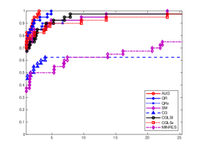
In Fig. 7 we compare all these direct methods with the iterative methods on the same set of matrices used for the performance profile in Fig. 5. It is clear that CG and MINRES show a much worse performance than the other solvers. On the other hand, even if AUG and QR remain slightly more robust and more efficient, the performance of the proposed iterative methods is close to that of direct backward stable methods.

Conclusion: The overall performance of the proposed iterative methods is close to that of standard direct backward stable methods.

8 Conclusions

We have considered both theoretical and practical aspects related to the solution of linear systems of the form Eq. 1. First, we have studied the structured condition number of the system and proposed a related explicit formula for its computation. Then, we have considered the numerical solution of Eq. 1. We have remarked that the same issues that deteriorate the performance of the Conjugate Gradient method on the normal equations also arise in this setting. This has guided us in the development of robust iterative methods for the numerical solution of Eq. 1. The new methods that have been proposed have been validated numerically. From the numerical experiments, we can draw the following conclusions:

• The choice of the $\epsilon$ parameter in CGLS$\epsilon$ deeply affects the performance of the method. A small value (approximately of order $10^{-14}$) is generally found a relevant choice, but a special attention is required in case of right-hand sides with large Euclidean norm.

• The proposed iterative methods are shown to be more stable than CG on the set of test problems considered.

• The first order estimates of the forward error obtained by the relative structured condition number are sharper estimates of the forward error, compared to standard bounds issued from linear system theory.

• The performance of the proposed methods, in terms of solution accuracy, is comparable to that of stable direct methods.

• For the considered class of linear systems, the best iterative solver appears to be CGLS$I$, that, compared to CGLS$\epsilon$, offers the advantage of being parameter free and more robust when solving problems exhibiting right-hand sides with large Euclidean norm.

References

- [1] M. Arioli, M. Baboulin, and S. Gratton, A partial condition number for linear least squares problems, SIAM J. Matrix Anal. Appl., 29 (2007), pp. 413–433, https://doi.org/10.1137/050643088, https://doi.org/10.1137/050643088, https://arxiv.org/abs/https://doi.org/10.1137/050643088.
- [2] A. Björck, Pivoting and stability in the augmented system method, in Numerical Analysis 1991, Proceedings of the 14th Dundee Conference, D. F. Griffiths and G. A. Watson, eds., vol. 260 of Pitman Research Notes in Mathematics, Longman Scientific and Technical, Essex, UK, 1992, pp. 1–16.
- [3] A. Björck, Numerical Methods for Least Squares Problems, vol. 51, SIAM, Philadelphia, 1996.
- [4] A. Björck, T. Elfving, and Z. Strakos, Stability of conjugate gradient and Lanczos methods for linear least squares problems, SIAM J. Matrix Anal. Appl., 19 (1998), pp. 720–736, https://doi.org/10.1137/S089547989631202X, http://dx.doi.org/10.1137/S089547989631202X.
- [5] H. Calandra, S. Gratton, E. Riccietti, and X. Vasseur, On high-order multilevel optimization strategies, arXiv e-prints, (2019), arXiv:1904.04692, p. arXiv:1904.04692, https://arxiv.org/abs/1904.04692.
- [6] H. Calandra, S. Gratton, E. Riccietti, and X. Vasseur, On the approximation of the solution of partial differential equations by artificial neural networks trained by a multilevel Levenberg-Marquardt method, arXiv e-prints, (2019), arXiv:1904.04685, p. arXiv:1904.04685, https://arxiv.org/abs/1904.04685.
- [7] X. W. Chang and D. Titley-Peloquin, Backward perturbation analysis for scaled total least-squares problems, Numer. Linear Algebra Appl., 16 (2009), pp. 627–648, https://doi.org/10.1002/nla.640, https://onlinelibrary.wiley.com/doi/abs/10.1002/nla.640, https://arxiv.org/abs/https://onlinelibrary.wiley.com/doi/pdf/10.1002/nla.640.
- [8] X. S. Chen, W. Li, X. Chen, and J. Liu, Structured backward errors for generalized saddle point systems, Linear Algebra Appl., 436 (2012), pp. 3109–3119, https://doi.org/https://doi.org/10.1016/j.laa.2011.10.012, http://www.sciencedirect.com/science/article/pii/S0024379511007063.
- [9] A. J. Cox and N. J. Higham, Backward error bounds for constrained least squares problems, BIT Numerical Mathematics, 39 (1999), pp. 210–227, https://doi.org/10.1023/A:1022385611904, https://doi.org/10.1023/A:1022385611904.
- [10] E. D. Dolan and J. J. Moré, Benchmarking optimization software with performance profiles, Mathematical Programming, 91 (2002), pp. 201–213, https://doi.org/10.1007/s101070100263, https://doi.org/10.1007/s101070100263.
- [11] I. S. Duff, N. I. M. Gould, J. K. Reid, J. A. Scott, and K. Turner, Factorization of sparse symmetric indefinite matrices, Technical Report RAL-90-066, (1990).
- [12] R. Estrin, D. Orban, and M. A. Saunders, LNLQ: An iterative method for least-norm problems with an error minimization property, in Cahier du GERAD No. G-2018-40, Montréal, Canada, 2018, http://web.stanford.edu/~restrin/files/eos2018.pdf.
- [13] R. Fletcher, A class of methods for nonlinear programming: III. Rates of convergence, Numerical Methods for Nonlinear Optimization, (1973).
- [14] V. Frayssé, S. Gratton, and V. Toumazou, Structured backward error and condition number for linear systems of the type , BIT Numerical Mathematics, 40 (2000), pp. 74–83, https://doi.org/10.1023/A:1022366318322, https://doi.org/10.1023/A:1022366318322.
- [15] P. E. Gill, W. Murray, D. B. Ponceleón, and M. A. Saunders, Solving reduced KKT systems in barrier methods for linear programming, in Numerical Analysis 1993, Proceedings of the 15th Dundee Conference, D. F. Griffiths and G. A. Watson, eds., vol. 303 of Pitman Research Notes in Mathematics, Longman Scientific and Technical, Essex, UK, 1994, pp. 89–104.
- [16] G. H. Golub and C. F. Van Loan, Matrix Computations, The Johns Hopkins University Press, USA, 2012. Fourth Edition.
- [17] S. Gratton, On the condition number of linear least squares problems in a weighted Frobenius norm, BIT Numerical Mathematics, 36 (1996), pp. 523–530, https://doi.org/10.1007/BF01731931, https://doi.org/10.1007/BF01731931.
- [18] A. Greenbaum, Estimating the attainable accuracy of recursively computed residual methods, SIAM J. Matrix Anal. Appl., 18 (1997), pp. 535–551, https://doi.org/10.1137/S0895479895284944, https://doi.org/10.1137/S0895479895284944, https://arxiv.org/abs/https://doi.org/10.1137/S0895479895284944.
- [19] N. J. Higham, Accuracy and Stability of Numerical Algorithms, vol. 80, SIAM, Philadelphia, 2002.
- [20] R. A. Horn and C. R. Johnson, Matrix Analysis, Cambridge University Press, 2012.
- [21] C. L. Lawson and R. J. Hanson, Solving Least Squares Problems, Prentice-Hall, Inc., Englewood Cliffs, New Jersey, USA, 1974. Fourth Edition.
- [22] X. G. Liu and N. Zhao, Linearization estimates of the backward errors for least squares problems, Numer. Linear Algebra Appl., 19 (2012), pp. 954–969, https://doi.org/10.1002/nla.827, https://onlinelibrary.wiley.com/doi/abs/10.1002/nla.827, https://arxiv.org/abs/https://onlinelibrary.wiley.com/doi/pdf/10.1002/nla.827.
- [23] J. Nocedal and S. Wright, Numerical Optimization, Springer-Verlag New York, 2006, https://doi.org/10.1007/978-0-387-40065-5. Second Edition.
- [24] C. C. Paige and M. A. Saunders, LSQR: An algorithm for sparse linear equations and sparse least squares, ACM Trans. Math. Softw., 8 (1982), pp. 43–71, https://doi.org/10.1145/355984.355989, http://doi.acm.org/10.1145/355984.355989.
- [25] J. Rice, A theory of condition, SIAM J. Numer. Anal., 3 (1966), pp. 287–310, https://doi.org/10.1137/0703023, https://doi.org/10.1137/0703023, https://arxiv.org/abs/https://doi.org/10.1137/0703023.
- [26] J. G. Sun, Structured backward errors for KKT systems, Linear Algebra Appl., 288 (1999), pp. 75–88, https://doi.org/https://doi.org/10.1016/S0024-3795(98)10184-2, http://www.sciencedirect.com/science/article/pii/S0024379598101842.
- [27] B. Walden, R. Karlson, and J. G. Sun, Optimal backward perturbation bounds for the linear least squares problem, Numer. Linear Algebra Appl., 2 (1995), pp. 271–286, https://doi.org/10.1002/nla.1680020308, https://onlinelibrary.wiley.com/doi/abs/10.1002/nla.1680020308, https://arxiv.org/abs/https://onlinelibrary.wiley.com/doi/pdf/10.1002/nla.1680020308.