Graph Structured Prediction Energy Networks

Abstract

For joint inference over multiple variables, a variety of structured prediction techniques have been developed to model correlations among variables and thereby improve predictions. However, many classical approaches suffer from one of two primary drawbacks: they either lack the ability to model high-order correlations among variables while maintaining computationally tractable inference, or they do not allow to explicitly model known correlations. To address this shortcoming, we introduce ‘Graph Structured Prediction Energy Networks,’ for which we develop inference techniques that allow to both model explicit local and implicit higher-order correlations while maintaining tractability of inference. We apply the proposed method to tasks from the natural language processing and computer vision domain and demonstrate its general utility.

1 Introduction

Many machine learning tasks involve joint prediction of a set of variables. For instance, semantic image segmentation infers the class label for every pixel in an image. To address joint prediction, it is common to use deep nets which model probability distributions independently over the variables (e.g., the pixels). The downside: correlations between different variables aren’t modeled explicitly.

A number of techniques, such as Structured SVMs [1], Max-Margin Markov Nets [2] and Deep Structured Models [3, 4], directly model relations between output variables. However, modeling the correlations between a large number of variables is computationally expensive and therefore generally impractical. As an attempt to address some of the fallbacks of classical high-order structured prediction techniques, Structured Prediction Energy Networks (SPENs) were introduced [5, 6]. SPENs assign a score to an entire prediction, which allows them to harness global structure. Additionally, because these models do not represent structure explicitly, complex relations between variables can be learned while maintaining tractability of inference. However, SPENs have their own set of downsides: Belanger and McCallum [5] mention, and we can confirm, that it is easy to overfit SPENs to the training data. Additionally, the inference techniques developed for SPENs do not enforce structural constraints among output variables, hence they cannot support structured scores and discrete losses. An attempt to combine locally structured scores with joint prediction was introduced very recently by Graber et al. [7]. However, Graber et al. [7] require the score function to take a specific, restricted form, and inference is formulated as a difficult-to-solve saddle-point optimization problem.

To address these concerns, we develop a new model which we refer to as ‘Graph Structured Prediction Energy Network’ (GSPEN). Specifically, GSPENs combine the capabilities of classical structured prediction models and SPENs and have the ability to explicitly model local structure when known or assumed, while providing the ability to learn an unknown or more global structure implicitly. Additionally, the proposed GSPEN formulation generalizes the approach by Graber et al. [7]. Concretely, inference in GSPENs is a maximization of a generally non-concave function w.r.t. structural constraints, for which we develop two inference algorithms.

We show the utility of GSPENs by comparing to related techniques on several tasks: optical character recognition, image tagging, multilabel classification, and named entity recognition. In general, we show that GSPENs are able to outperform other models. Our implementation is available at https://github.com/cgraber/GSPEN.

2 Background

Let $x\in\mathcal{X}$ represent the input provided to a model, such as a sentence or an image. In this work, we consider tasks where the outputs take the form $y=(y_{1},\dots,y_{K})\in\mathcal{Y}\coloneqq\prod_{k=1}^{K}\mathcal{Y}_{k}$, i.e., they are vectors where the $k$-th variable’s domain is the discrete and finite set $\mathcal{Y}_{k}=\{1,\ldots,|\mathcal{Y}_{k}|\}$. In general, the number of variables $K$ which are part of the configuration $y$ can depend on the observation $x$. However, for readability only, we assume all $y\in\mathcal{Y}$ contain $K$ entries, i.e., we drop the dependence of the output space $\mathcal{Y}$ on input $x$.

All models we consider consist of a function $F(x,y;w)$, which assigns a score to a given configuration $y$ conditioned on input $x$ and is parameterized by weights $w$. Provided an input $x$, the inference problem requires finding the configuration $\hat{y}$ that maximizes this score, i.e., $\hat{y}\coloneqq\operatorname*{arg\,max}_{y\in\mathcal{Y}}F(x,y;w)$.

To find the parameters $w$ of the function $F(x,y;w)$, it is common to use a Structured Support Vector Machine (SSVM) (a.k.a. Max-Margin Markov Network) objective [1, 2]: given a multiset $\left\{\left(x^{i},y^{i}\right)_{i=1}^{N}\right\}$ of data points $\left(x^{i},y^{i}\right)$ comprised of an input $x^{i}$ and the corresponding ground-truth configuration $y^{i}$, a SSVM attempts to find weights $w$ which maximize the margin between the scores assigned to the ground-truth configuration $y^{i}$ and the inference prediction:

$$\min_{w}\sum_{\left(x^{i},y^{i}\right)}\max_{\hat{y}\in\mathcal{Y}}\left\{F\left(x^{i},\hat{y};w\right)+L\left(\hat{y},y^{i}\right)\right\}-F\left(x^{i},y^{i};w\right).$$ (1)

Hereby, $L\left(\hat{y},y^{i}\right)$ is a task-specific and often discrete loss, such as the Hamming loss, which steers the model towards learning a margin between correct and incorrect outputs. Due to addition of the task-specific loss $L(\hat{y},y^{i})$ to the model score $F\left(x^{i},\hat{y};w\right)$, we often refer to the maximization task within Eq. (1) as loss-augmented inference. The procedure to solve loss-augmented inference depends on the considered model, which we discuss next.

Unstructured Models. Unstructured models, such as feed-forward deep nets, assign a score to each label of variable $y_{k}$ which is part of the configuration $y$, irrespective of the label choice of other variables. Hence, the final score function $F$ is the sum of $K$ individual scores $f_{k}(x,y_{k};w)$, one for each variable:

$$F(x,y;w)\coloneqq\sum_{k=1}^{K}f_{k}(x,y_{k};w).$$ (2)

Because the scores for each output variable do not depend on the scores assigned to other output variables, the inference assignment is determined efficiently by independently finding the maximum score for each variable $y_{k}$. The same is true for loss-augmented inference, assuming that the loss decomposes into a sum of independent terms as well.

Classical Structured Models. Classical structured models incorporate dependencies between variables by considering functions that take more than one output space variable $y_{k}$ as input, i.e., each function depends on a subset $r\subseteq\{1,\dots,K\}$ of the output variables. We refer to the subset of variables via $y_{r}=(y_{k})_{k\in r}$ and use $f_{r}$ to denote the corresponding function. The overall score for a configuration $y$ is a sum of these functions, i.e.,

$$F(x,y;w)\coloneqq\sum_{r\in\mathcal{R}}f_{r}(x,y_{r};w).$$ (3)

Hereby, $\mathcal{R}$ is a set containing all of the variable subsets which are required to compute $F$. The variable subset relations between functions $f_{r}$, i.e., the structure, is often visualized using factor graphs or, generally, Hasse diagrams.

This formulation allows to explicitly model relations between variables, but it comes at the price of more complex inference which is NP-hard [8] in general. A number of approximations to this problem have been developed and utilized successfully (see Sec. 5 for more details), but the complexity of these methods scales with the size of the largest region $r$. For this reason, these models commonly consider only unary and pairwise regions, i.e., regions with one or two variables.

Inference, i.e., maximization of the score, is equivalent to the integer linear program

$$\max_{p\in\mathcal{M}}\sum_{r\in\mathcal{R}}\sum_{y_{r}\in\mathcal{Y}_{r}}p_{r}(y_{r})f_{r}(x,y_{r};w),$$ (4)

where each $p_{r}$ represents a marginal probability vector for region $r$ and $\mathcal{M}$ represents the set of $p_{r}$ whose marginal distributions are globally consistent, which is often called the marginal polytope. Adding an entropy term over the probabilities to the inference objective transforms the problem from maximum a-posteriori (MAP) to marginal inference, and pushes the predictions to be more uniform [9, 10]. When combined with the learning procedure specified above, this entropy provides learning with the additional interpretation of maximum likelihood estimation [9]. The training objective then also fits into the framework of Fenchel-Young Losses [11].

For computational reasons, it is common to relax the marginal polytope $\mathcal{M}$ to the local polytope $\mathcal{M}_{L}$, which is the set of all probability vectors that marginalize consistently for the factors present in the graph [9]. Since the resulting marginals are no longer globally consistent, i.e., they are no longer guaranteed to arise from a single joint distribution, we write the predictions for each region using $b_{r}(y_{r})$ instead of $p_{r}(y_{r})$ and refer to them using the term “beliefs.” Additionally, the entropy term is approximated using fractional entropies [12] such that it only depends on the factors in the graph, in which case it takes the form $H_{\mathcal{R}}(b)\coloneqq\sum_{r\in\mathcal{R}}\sum_{y_{r}\in\mathcal{Y}_{r}}-b_{r}(y_{r})\log b_{r}(y_{r})$.

Structured Prediction Energy Networks. Structured Prediction Energy Networks (SPENs) [5] were motivated by the desire to represent interactions between larger sets of output variables without incurring a high computational cost. The SPEN score function takes the following form:

$$F(x,p_{1},\dots,p_{K};w)\coloneqq T\left(\bar{f}(x;w),p_{1},\dots,p_{K};w\right),$$ (5)

where $\bar{f}(x;w)$ is a learned feature representation of the input $x$, each $p_{k}$ is a one-hot vector, and $T$ is a function that takes these two terms and assigns a score. This representation of the labels, i.e., $p_{k}$, is used to facilitate gradient-based optimization during inference. More specifically, inference is formulated via the program:

$$\max_{p_{k}\in\Delta_{k}\forall k}T\left(\bar{f}(x;w),p_{1},\dots,p_{K};w\right),$$ (6)

where each $p_{k}$ is constrained to lie in the $|\mathcal{Y}_{k}|$-dimensional probability simplex $\Delta_{k}$. This task can be solved using any constrained optimization method. However, for non-concave $T$ the inference solution might only be approximate.

NLStruct. SPENs do not support score functions that contain a structured component. In response, Graber et al. [7] introduced NLStruct, which combines a classical structured score function with a nonlinear transformation applied on top of it to produce a final score. Given a set $\mathcal{R}$ as defined previously, the NLStruct score function takes the following form:

$$F(x,p_{\mathcal{R}};w)\coloneqq T\left(f_{\mathcal{R}}(x;w)\circ p_{\mathcal{R}};w\right),$$ (7)

where $f_{\mathcal{R}}(x;w)\coloneqq(f_{r}(x,y_{r};w))|_{r\in\mathcal{R},y_{r}\in\mathcal{Y}_{r}}$ is a vectorized form of the score function for a classical structured model, $p_{\mathcal{R}}\coloneqq(p_{r}(y_{r}))|_{\forall r\in\mathcal{R},\forall y_{r}\in\mathcal{Y}_{r}}$ is a vector containing all marginals, ‘$\circ$’ is the Hadamard product, and $T$ is a scalar-valued function.

For this model, inference is formulated as a constrained optimization problem, where $\mathcal{Y}_{\mathcal{R}}\coloneqq\prod_{r\in\mathcal{R}}\mathcal{Y}_{r}$:

$$\max_{y\in\mathbb{R}^{|\mathcal{Y}_{\mathcal{R}}|},p_{\mathcal{R}}\in\mathcal{M}}T(y;w)\text{~{}~{}s.t.~{}~{}}y=f_{\mathcal{R}}(x;w)\circ p_{\mathcal{R}}.$$ (8)

Forming the Lagrangian of this program and rearranging leads to the saddle-point inference problem

$$\min_{\lambda}\max_{y}\left\{T(y;w)-\lambda^{T}y\right\}+\max_{p_{\mathcal{R}}\in\mathcal{M}}\lambda^{T}\left(f_{\mathcal{R}}(x;w)\circ p_{\mathcal{R}}\right).$$ (9)

Notably, maximization over $p_{\mathcal{R}}$ is solved using techniques developed for classical structured models, and the saddle-point problem is optimized using the primal-dual algorithm of Chambolle and Pock [13], which alternates between updating $\lambda$, $y$, and $p_{\mathcal{R}}$.

3 Graph Structured Prediction Energy Nets

Graph Structured Prediction Energy Networks (GSPENs) generalize all aforementioned models. They combine both a classical structured component as well as a SPEN-like component to score an entire set of predictions jointly. Additionally, the GSPEN score function is more general than that for NLStruct, and includes it as a special case. After describing the formulation of both the score function and the inference problem (Sec. 3.1), we discuss two approaches to solving inference (Sec. 3.2 and Sec. 3.3) that we found to work well in practice. Unlike the methods described previously for NLStruct, these approaches do not require solving a saddle-point optimization problem.

3.1 GSPEN Model

The GSPEN score function is written as follows:

$$F\left(x,p_{\mathcal{R}};w\right)\coloneqq T\left(\bar{f}(x;w),p_{\mathcal{R}};w\right),$$

where vector $p_{\mathcal{R}}\coloneqq(p_{r}(y_{r}))|_{r\in\mathcal{R},y_{r}\in\mathcal{Y}_{r}}$ contains one marginal per region per assignment of values to that region. This formulation allows for the use of a structured score function while also allowing $T$ to score an entire prediction jointly. Hence, it is a combination of classical structured models and SPENs. For instance, we can construct a GSPEN model by summing a classical structured model and a multilayer perceptron that scores an entire label vector, in which case the score function takes the form $F(x,p_{\mathcal{R}};w)\coloneqq\sum_{r\in\mathcal{R}}\sum_{y_{r}\in\mathcal{Y}_{r}}p_{r}(y_{r})f_{r}(x,y_{r};w)+\text{MLP}\left(p_{\mathcal{R}};w\right)$. Of course, this is one of many possible score functions that are supported by this formulation. Notably, we recover the NLStruct score function if we use $T(\bar{f}(x;w),p_{\mathcal{R}};w)=T^{\prime}(\bar{f}(x;w)\circ p_{\mathcal{R}};w)$ and let $\bar{f}(x;w)=f_{\mathcal{R}}(x;w)$.

Given this model, the inference problem is

$$\max_{p_{\mathcal{R}}\in\mathcal{M}}T\left(\bar{f}(x;w),p_{\mathcal{R}};w\right).$$ (10)

As for classical structured models, the probabilities are constrained to lie in the marginal polytope. In addition we also consider a fractional entropy term over the predictions, leading to

$$\max_{p_{\mathcal{R}}\in\mathcal{M}}T\left(\bar{f}(x;w),p_{\mathcal{R}};w\right)+H_{\mathcal{R}}(p_{\mathcal{R}}).$$ (11)

In the classical setting, adding an entropy term relates to Fenchel duality [11]. However, the GSPEN inference objective does not take the correct form to use this reasoning. We instead view this entropy as a regularizer for the predictions: it pushes predictions towards a uniform distribution, smoothing the inference objective, which we empirically observed to improve convergence. The results discussed below indicate that adding entropy leads to better-performing models. Also note that it is possible to add a similar entropy term to the SPEN inference objective, which is mentioned by Belanger and McCallum [5] and Belanger et al. [6].

For inference in GSPEN, SPEN procedures cannot be used since they do not maintain the additional constraints imposed by the graphical model, i.e., the marginal polytope ${\cal M}$. We also cannot use the inference procedure developed for NLStruct, as the GSPEN score function does not take the same form. Therefore, in the following, we describe two inference algorithms that optimize the program while maintaining structural constraints.

3.2 Frank-Wolfe Inference

Algorithm 1 Frank-Wolfe Inference for GSPEN

1:  Input: Initial set of predictions $p_{\mathcal{R}}$; Input $x$;    Factor graph $\mathcal{R}$

2:  for $t=1\dots T$ do

3:     $g\Leftarrow\nabla_{p_{\mathcal{R}}}F(x,p_{\mathcal{R}};w)$

4:     $\widehat{p}_{\mathcal{R}}\Leftarrow\max\limits_{\widehat{p}_{\mathcal{R}}\in\mathcal{M}_{\mathcal{R}}}\sum\limits_{r\in\mathcal{R},y_{r}\in\mathcal{Y}_{r}}\hat{p}_{r}(y_{r})g_{r}(y_{r})$

5:     $p_{\mathcal{R}}\Leftarrow p_{\mathcal{R}}+\frac{1}{t}\left(\widehat{p}_{\mathcal{R}}-p_{\mathcal{R}}\right)$

6:  end for

7:  Return: $p_{\mathcal{R}}$

Algorithm 2 Structured Entropic Mirror Descent Inference

1:  Input: Initial set of predictions $p_{\mathcal{R}}$; Input $x$;    Factor graph $\mathcal{R}$

2:  for $t=1\dots T$ do

3:     $g\Leftarrow\nabla_{p_{\mathcal{R}}}F\left(x,p_{\mathcal{R}};w\right)$

4:     $a\Leftarrow 1+\ln p_{\mathcal{R}}+g/\sqrt{t}$

5:     $p_{\mathcal{R}}\Leftarrow\max\limits_{\hat{p}_{\mathcal{R}}\in\mathcal{M}}\sum\limits_{r\in\mathcal{R},y_{r}\in\mathcal{Y}_{r}}\hat{p}_{r}(y_{r})a_{r}(y_{r})\!\!+\!\!H_{\mathcal{R}}(\hat{p}_{\mathcal{R}})$

6:  end for

7:  Return: $p_{\mathcal{R}}$

The Frank-Wolfe algorithm [14] is suitable because the objectives in Eqs. (10, 11) are non-linear while the constraints are linear. Specifically, using [14], we compute a linear approximation of the objective at the current iterate, maximize this linear approximation subject to the constraints of the original problem, and take a step towards this maximum.

In Algorithm 1 we detail the steps to optimize Eq. (10). In every iteration we first calculate the gradient of the score function $F$ with respect to the marginals/beliefs using the current prediction as input. We denote this gradient using $g=\nabla_{p_{\mathcal{R}}}T\left(\bar{f}(x;w),p_{\mathcal{R}};w\right)$. The gradient of $T$ depends on the specific function used and is computed via backpropagation. If entropy is part of the objective, an additional term of $-\ln\left(p_{\mathcal{R}}\right)-1$ is added to this gradient.

Next we find the maximizing beliefs which is equivalent to inference for classical structured prediction: the constraint space is identical and the objective is a linear function of the marginals/beliefs. Hence, we solve this inner optimization using one of a number of techniques referenced in Sec. 5.

Convergence guarantees for Frank-Wolfe have been proven when the overall objective is concave, continuously differentiable, and has bounded curvature [15], which is the case when $T$ has these properties with respect to the marginals. This is true even when the inner optimization is only solved approximately, which is often the case due to standard approximations used for structured inference. When $T$ is non-concave, convergence can still be guaranteed, but only to a local optimum [16]. Note that entropy has unbounded curvature, therefore its inclusion in the objective precludes convergence guarantees. Other variants of the Frank-Wolfe algorithm exist which improve convergence in certain cases [17, 18]. We defer a study of these properties to future work.

3.3 Structured Entropic Mirror Descent

Mirror descent, another constrained optimization algorithm, is analogous to projected subgradient descent, albeit using a more general distance beyond the Euclidean one [19]. This algorithm has been used in the past to solve inference for SPENs, where entropy was used as the link function $\psi$ and by normalizing over each coordinate independently [5]. We similarly use entropy in our case. However, the additional constraints in form of the polytope ${\cal M}$ require special care.

$$\min_{w}\sum_{\left(x^{(i)},p_{\mathcal{R}}^{(i)}\right)}\left[\max_{\hat{p}_{\mathcal{R}}\in\mathcal{M}}\left\{T\left(\bar{f}(x;w),\hat{p}_{\mathcal{R}};w\right)+L\left(\hat{p}_{\mathcal{R}},p_{\mathcal{R}}^{(i)}\right)\right\}-T\left(\bar{f}\left(x^{(i)};w\right),p_{\mathcal{R}}^{(i)};w\right)\right]_{+}$$

Figure 1: The GSPEN learning formulation, consisting of a Structured SVM (SSVM) objective with loss-augmented inference. Note that each $p_{\mathcal{R}}^{(i)}$ are one-hot representations of labels $y_{i}$.

We summarize the structured entropic mirror descent inference for the proposed model in Algorithm 2. Each iteration of mirror descent updates the current prediction $p_{\mathcal{R}}$ and dual vector $a$ in two steps: (1) $a$ is updated based on the current prediction $p_{\mathcal{R}}$. Using $\psi(p_{\mathcal{R}})=-H_{\mathcal{R}}(p_{\mathcal{R}})$ as the link function, this update step takes the form $a=1+\ln p_{\mathcal{R}}+\frac{1}{\sqrt{t}}\left(\nabla_{p_{\mathcal{R}}}T\left(\bar{f}(x;w),p_{\mathcal{R}};w\right)\right)$. As mentioned previously, the gradient of $T$ can be computed using backpropagation; (2) $p_{\mathcal{R}}$ is updated by computing the maximizing argument of the Fenchel conjugate of the link function $\psi^{*}$ evaluated at $a$. More specifically, $p_{\mathcal{R}}$ is updated via

$$p_{\mathcal{R}}=\max_{\hat{p}_{\mathcal{R}}\in\mathcal{M}}\sum_{r\in\mathcal{R}}\sum_{y_{r}\in\mathcal{Y}_{r}}\hat{p}_{r}(y_{r})a_{r}(y_{r})+H_{\mathcal{R}}\left(\hat{p}_{\mathcal{R}}\right),$$ (12)

which is identical to classical structured prediction.

When the inference objective is concave and Lipschitz continuous (i.e., when $T$ has these properties), this algorithm has also been proven to converge [19]. Unfortunately, we are not aware of any convergence results if the inner optimization problem is solved approximately and if the objective is not concave. In practice, though, we did not observe any convergence issues during experimentation.

3.4 Learning GSPEN Models

GSPENs assign a score to an input $x$ and a prediction $p$. An SSVM learning objective is applicable, which maximizes the margin between the scores assigned to the correct prediction and the inferred result. The full SSVM learning objective with added loss-augmented inference is summarized in Fig. 1. The learning procedure consists of computing the highest-scoring prediction using one of the inference procedures described in Sec. 3.2 and Sec. 3.3 for each example in a mini-batch and then updating the weights of the model towards making better predictions.

4 Experiments

	Struct	SPEN	NLStruct	GSPEN
OCR (size 1000)	0.40 s	0.60 s	68.56 s	8.41 s
Tagging	18.85 s	30.49 s	208.96 s	171.65 s
Bibtex	0.36 s	11.75 s	–	13.87 s
Bookmarks	6.05 s	94.44 s	–	234.33 s
NER	29.16 s	–	–	99.83 s

Table 1: Average time to compute inference objective and complete a weight update for one pass through the training data. We show all models trained for this work.

To demonstrate the utility of our model and to compare inference and learning settings, we report results on the tasks of optical character recognition (OCR), image tagging, multilabel classification, and named entity recognition (NER). For each experiment, we use the following baselines: Unary is an unstructured model that does not explicitly model the correlations between output variables in any way. Struct is a classical deep structured model using neural network potentials. We follow the inference and learning formulation of [3], where inference consists of a message passing algorithm derived using block coordinate descent on a relaxation of the inference problem. SPEN and NLStruct represent the formulations discussed in Sec. 2. Finally, GSPEN represents Graph Structured Prediction Energy Networks, described in Sec. 3. For GSPENs, the inner structured inference problems are solved using the same algorithm as for Struct. To compare the run-time of these approaches, Table 1 gives the average epoch compute time (i.e., time to compute the inference objective and update model weights) during training for our models for each task. In general, GSPEN training was more efficient with respect to time than NLStruct but, expectedly, more expensive than SPEN. Additional experimental details, including hyper-parameter settings, are provided in Appendix A.2.

4.1 Optical Character Recognition (OCR)

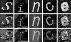
Figure 2: OCR sample data points with different interpolation factors $\alpha$.

For the OCR experiments, we generate data by selecting a list of 50 common 5-letter English words, such as ‘close,’ ‘other,’ and ‘world.’ To create each data point, we choose a word from this list and render each letter as a 28x28 pixel image by selecting a random image of the letter from the Chars74k dataset [20], randomly shifting, scaling, rotating, and interpolating with a random background image patch. A different pool of backgrounds and letter images was used for the training, validation, and test splits of the data. The task is to identify the words given 5 ordered images. We create three versions of this dataset using different interpolation factors of $\alpha\in\{0.3,0.5,0.7\}$, where each pixel in the final image is computed as $\alpha x_{\text{background}}+(1-\alpha)x_{\text{letter}}$. See Fig. 2 for a sample from each dataset. This process was deliberately designed to ensure that information about the structure of the problem (i.e., which words exist in the data) is a strong signal, while the signal provided by each individual letter image can be adjusted. The training, validation, and test set sizes for each dataset are 10,000, 2,000, and 2,000, respectively. During training we vary the training data to be either 200, 1k or 10k.

To study the inference algorithm, we train four different GSPEN models on the dataset containing 1000 training points and using $\alpha=0.5$. Each model uses either Frank-Wolfe or Mirror Descent and included/excluded the entropy term. To maintain tractability of inference, we fix a maximum iteration count for each model. We additionally investigate the effect of this maximum count on final performance. Additionally, we run this experiment by initializing from two different Struct models, one being trained using entropy during inference and one being trained without entropy. The results for this set of experiments are shown in Fig. 3(a). Most configurations perform similarly across the number of iterations, indicating these choices are sufficient for convergence. When initializing from the models trained without entropy, we observe that both Frank-Wolfe without entropy and Mirror Descent with entropy performed comparably. When initializing from a model trained with entropy, the use of mirror descent with entropy led to much better results.

The results for all values of $\alpha$ using a train dataset size of 1000 are presented in Fig. 3(b), and results for all train dataset sizes with $\alpha=0.5$ are presented in Fig. 3(c). We observe that, in all cases, GSPEN outperforms all baselines. The degree to which GSPEN outperforms other models depends most on the amount of train data: with a sufficiently large amount of data, SPEN and GSPEN perform comparably. However, when less data is provided, GSPEN performance does not drop as sharply as that of SPEN initially. It is also worth noting that GSPEN outperformed NLStruct by a large margin. The NLStruct model is less stable due to its saddle-point formulation. Therefore it is much harder to obtain good performance with this model.

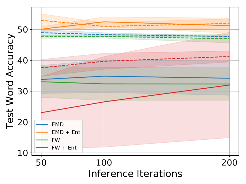
(a)

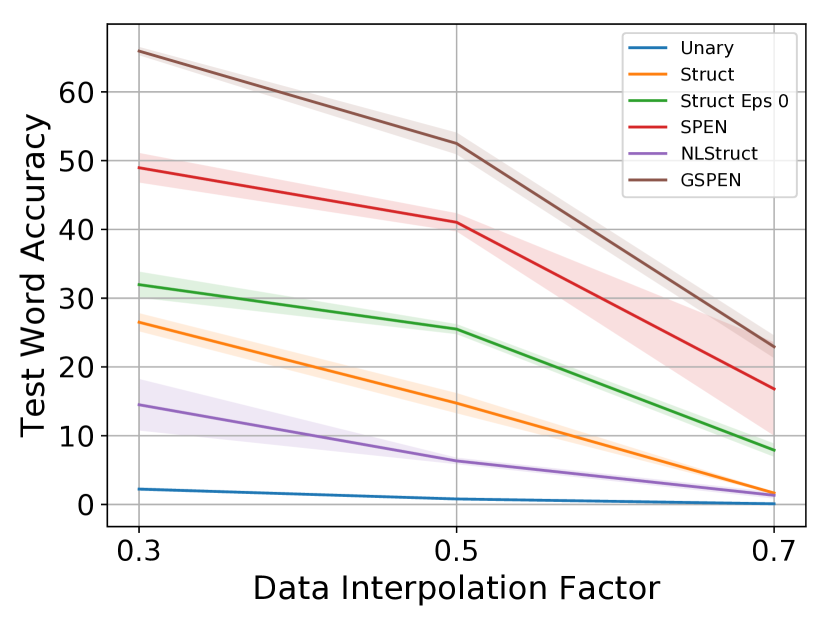
(b)

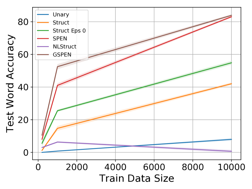
(c)

Figure 3: Experimental results on OCR data. The dashed lines in (a) represent models trained from Struct without entropy, while solid lines represent models trained from Struct with entropy.

4.2 Image Tagging

Next, we evaluate on the MIRFLICKR25k dataset [21], which consists of 25,000 images taken from Flickr. Each image is assigned a subset of 24 possible tags. The train/val/test sets for these experiments consist of 10,000/5,000/10,000 images, respectively.

We compare to NLStruct and SPEN. We initialize the structured portion of our GSPEN model using the pre-trained DeepStruct model described by Graber et al. [7], which consists of unary potentials produced from an AlexNet architecture [22] and linear pairwise potentials of the form $f_{i,j}(y_{i},y_{j},W)=W_{i,j,x_{i},x_{j}}$, i.e., containing one weight per pair in the graph per assignment of values to that pair. A fully-connected pairwise graph was used. The $T$ function for our GSPEN model consists of a 2-layer MLP with 130 hidden units. It takes as input a concatenation of the unary potentials generated by the AlexNet model and the current prediction. Additionally, we train a SPEN model with the same number of layers and hidden units. We used Frank-Wolfe without entropy for both SPEN and GSPEN inference.

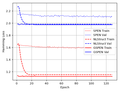
Figure 4: Results for image tagging.

The results are shown in Fig. 4. GSPEN obtains similar test performance to the NLStruct model, and both outperform SPEN. However, the NLStruct model was run for 100 iterations during inference without reaching ‘convergence’ (change of objective smaller than threshold), while the GSPEN model required an average of 69 iterations to converge at training time and 52 iterations to converge at test time. Our approach has the advantage of requiring fewer variables to maintain during inference and requiring fewer iterations of inference to converge. The final test losses for SPEN, NLStruct and GSPEN are 2.158, 2.037, and 2.029, respectively.

4.3 Multilabel Classification

We use the Bibtex and Bookmarks multilabel datasets [23]. They consist of binary-valued input feature vectors, each of which is assigned some subset of 159/208 possible labels for Bibtex/Bookmarks, respectively. We train unary and SPEN models with architectures identical to [5] and [24] but add dropout layers. In addition, we further regularize the unary model by flipping each bit of the input vectors with probability 0.01 when sampling mini-batches. For Struct and GSPEN, we generate a graph by first finding the label variable that is active in most training data label vectors and add edges connecting every other variable to this most active one. Pairwise potentials are generated by passing the input vector through a 2-layer MLP with 1k hidden units. The GSPEN model is trained by starting from the SPEN model, fixing its parameters, and training the pairwise potentials.

The results are in Table 2 alongside those taken from [5] and [24]. We found the Unary models to perform similarly to or better than previous best results. Both SPEN and Struct are able to improve upon these Unary results. GSPEN outperforms all configurations, suggesting that the contributions of the SPEN component and the Struct component to the score function are complementary.

4.4 NER

We also assess suitability for Named Entity Recognition (NER) using the English portion of the CoNLL 2003 shared task [25]. To demonstrate the applicability of GSPEN for this task, we transformed two separate models, specifically the ones presented by Ma and Hovy [26] and Akbik et al. [27], into GSPENs by taking their respective score functions and adding a component that jointly scores an entire set of predictions. In each case, we first train six instances of the structured model using different random initializations and drop the model that performs the worst on validation data. We then train the GSPEN model, initializing the structured component from these pre-trained models.

The final average performance is presented in Table 3, and individual trial information can be found in Table 4 in the appendix. When comparing to the model described by Ma and Hovy [26], GSPEN improves the final test performance in four out of the five trials, and GSPEN has a higher overall average performance across both validation and test data. Compared to Akbik et al. [27], on average GSPEN’s validation score was higher, but it performed slightly worse at test time. Overall, these results demonstrate that it is straightforward to augment a task-specific structured model with an additional prediction scoring function which can lead to improved final task performance.

Table 2: Multilabel classification results for all models. All entries represent macro F1 scores. The top results are taken from the cited publications. Bibtex Bookmarks Validation Test Validation Test SPEN [5] – 42.2 – 34.4 DVN [24] – 44.7 – 37.1 Unary 43.3 44.1 38.4 37.4 Struct 45.8 46.1 39.7 38.9 SPEN 46.6 46.5 40.2 39.2 GSPEN 47.5 48.6 41.2 40.7

Table 3: Named Entity Recognition results for all models. All entries represent F1 scores averaged over five trials. Avg. Val. Avg. Test Struct [26] 94.88 $\pm$ 0.18 91.37 $\pm$ 0.04 + GSPEN 94.97 $\pm$ 0.16 91.51 $\pm$ 0.17 Struct [27] 95.88 $\pm$ 0.10 92.79 $\pm$ 0.08 + GSPEN 95.96 $\pm$ 0.08 92.69 $\pm$ 0.17

5 Related Work

A variety of techniques have been developed to model structure among output variables, originating from seminal works of [28, 2, 1]. These works focus on extending linear classification, both probabilistic and non-probabilistic, to model the correlation among output variables. Generally speaking, scores representing both predictions for individual output variables and for combinations of output variables are used. A plethora of techniques have been developed to solve inference for problems of this form, e.g., [29, 30, 31, 32, 33, 34, 35, 36, 37, 38, 39, 9, 40, 41, 42, 43, 44, 45, 46, 47, 48, 49, 50, 51, 52, 53, 12, 54, 55, 56, 57, 58, 59, 60, 61, 62]. As exact inference for general structures is NP-hard [8], early work focused on tractable exact inference. However, due to interest in modeling problems with intractable structure, a plethora of approaches have been studied for learning with approximate inference [63, 64, 65, 66, 67, 68, 69, 70]. More recent work has also investigated the role of different types of prediction regularization, with Niculae et al. [10] replacing the often-used entropy regularization with an L2 norm and Blondel et al. [11] casting both as special cases of a Fenchel-Young loss framework.

To model both non-linearity and structure, deep learning and structured prediction techniques were combined. Initially, local, per-variable score functions were learned with deep nets and correlations among output variables were learned in a separate second stage [71, 72]. Later work simplified this process, learning both local score functions and variable correlations jointly [73, 74, 3, 4, 75].

Structured Prediction Energy Networks (SPENs), introduced by Belanger and McCallum [5], take a different approach to modeling structure. Instead of explicitly specifying a structure a-priori and enumerating scores for every assignment of labels to regions, SPENs learn a function which assigns a score to an input and a label. Inference uses gradient-based optimization to maximize the score w.r.t. the label. Belanger et al. [6] extend this technique by unrolling inference in a manner inspired by Domke [76]. Both approaches involve iterative inference procedures, which are slower than feed-forward prediction of deep nets. To improve inference speed, Tu and Gimpel [77] learn a neural net to produce the same output as the gradient-based methods. Deep Value Networks [24] follow the same approach of Belanger and McCallum [5] but use a different objective that encourages the score to equal the task loss of the prediction. All these approaches do not permit to include known structure. The proposed approach enables this.

Our approach is most similar to our earlier work [7], which combines explicitly-specified structured potentials with a SPEN-like score function. The score function of our earlier work is a special case of the one presented here. In fact, earlier we required a classical structured prediction model as an intermediate layer of the score function, while we don’t make this assumption any longer. Additionally, in our earlier work we had to solve inference via a computationally challenging saddle-point objective. Another related approach is described by Vilnis et al. [78], whose score function is the sum of a classical structured score function and a (potentially non-convex) function of the marginal probability vector $p_{\mathcal{R}}$. This is also a special case of the score function presented here. Additionally, the inference algorithm they develop is based on regularized dual averaging [79] and takes advantage of the structure of their specific score function, i.e., it is not directly applicable to our setting.

6 Conclusions

The developed GSPEN model combines the strengths of several prior approaches to solving structured prediction problems. It allows machine learning practitioners to include inductive bias in the form of known structure into a model while implicitly capturing higher-order correlations among output variables. The model formulation described here is more general than previous attempts to combine explicit local and implicit global structure modeling while not requiring inference to solve a saddle-point problem.

Acknowledgments

This work is supported in part by NSF under Grant No. 1718221 and MRI #1725729, UIUC, Samsung, 3M, Cisco Systems Inc. (Gift Award CG 1377144) and Adobe. We thank NVIDIA for providing GPUs used for this work and Cisco for access to the Arcetri cluster.

Appendix A Appendix

In this Appendix, we first present additional experimental results for the NER before providing additional details on experiments, including model architectures and selection of hyper-parameters.

A.1 Additional Experimental Results

Table 4: All Trials for NER experiments.

	Ma and Hovy [26]		+ GSPEN
Trial	Val. F1	Test F1	Val. F1	Test F1
$1$	$94.94$	$91.36$	$94.85$	$91.25$
$2$	$94.67$	$91.37$	$94.76$	$91.53$
$3$	$94.74$	$91.32$	$95.07$	$91.60$
$4$	$94.94$	$91.35$	$95.08$	$91.47$
$5$	$95.12$	$91.44$	$95.10$	$91.71$
	Akbik et al. [27]		+ GSPEN
$1$	$0.9576$	$0.9284$	$0.9587$	$0.9288$
$2$	$0.9601$	$0.9277$	$0.9599$	$0.9246$
$3$	$0.9581$	$0.9271$	$0.9588$	$0.9271$
$4$	$0.9592$	$0.9291$	$0.9600$	$0.9280$
$5$	$0.9590$	$0.9272$	$0.9604$	$0.9260$

Table 4 contains the results for all trials of the NER experiments. When comparing to Ma and Hovy [26], we outperform their model on both validation and test data in four out of five trials. When comparing to Akbik et al. [27], we outperform their model on validation data in four out of five trials, but only outperform their model on test data in one trial.

A.2 Additional Experimental Details

General Details:

Unless otherwise specified, all Struct models were trained by using the corresponding pre-trained Unary model, fixing these parameters, and training pairwise potentials. All SPEN models were trained by using the pre-trained Unary model, fixing these parameters, and training the $T$ function. Early stopping based on task performance on validation was used to select the number of epochs for training. For SPEN, GSPEN, and Struct models, loss-augmented inference was used where the loss function equals the sum of the $0$-$1$ losses per output variable, i.e., $L(\hat{y},y)~{}\coloneqq~{}\sum_{i=1}^{n}~{}\mathbf{1}[\hat{y}_{i}~{}\neq~{}y_{i}]$ where $n$ is the number of output variables.

OCR:

The Unary model is a single $3$-layer multilayer perceptron (MLP) with ReLU activations, hidden layer sizes of $200$, and a dropout layer after the first linear layer with keep probability $0.5$. Scores for each image were generated by independently passing them into this network. Both Struct and GSPEN use a graph with one pairwise region per pair of adjacent letters, for a total of $4$ pairs. Linear potentials are used, containing one entry per pair per set of assignments of values to each pair. The score function for both SPEN and GSPEN takes the form $F(x,p;w)=\sum_{r\in\mathcal{R}}\sum_{y_{r}\in\mathcal{Y}_{r}}p_{r}(y_{r})b_{r}(x,y_{;}w)+T(B(x),p)$, where in the SPEN case $\mathcal{R}$ contains only unary regions and in the GSPEN case $\mathcal{R}$ consists of the graph used by Struct. Each $b_{r}$ represents the outputs of the same model as Unary/Struct for SPEN/GSPEN, respectively, and $B(x)$ represents the vector $(b_{r}(x,y_{i};w)|_{y_{r}\in\mathcal{Y}_{r}})$. For every SPEN and GSPEN model trained, $T$ is a $2$-layer MLP with softplus activations, an output size of $1$, and either $500$, $1000$, or $2000$ hidden units. These hidden sizes as well as the number of epochs of training for each model were determined based on task performance on the validation data. Message-passing inference used in both Struct and GSPEN ran for $10$ iterations. GSPEN models were trained by using the pre-trained Struct model, fixing these parameters, and training the $T$ function. The NLStruct model consisted of a $2$-layer MLP with $2834$ hidden units, an output size of $1$, and softplus activations. We use the same initialization described by Graber et al. [7] for their word recognition experiments, where the first linear layer was initialized to the identity matrix and the second linear layer was initialized to a vector of all 1s. NLStruct models were initialized from the Struct models trained without entropy and used fixed potentials. The inference configuration described by Graber et al. [7] was used, where inference was run for $100$ iterations with averaging applied over the final $50$ iterations.

All settings for the OCR experiments used a mini-batch size of $128$ and used the Adam optimizer, with Unary, SPEN, and GSPEN using a learning rate of $10^{-4}$ and Struct using a learning rate of $10^{-3}$. Gradients were clipped to a norm of $1$ before updates were applied. Inference in both SPEN and GSPEN were run for a maximum of $100$ iterations. Inference was terminated early for both models if the inference objective for all datapoints in the minibatch being processed changed by less than $0.0001$.

Three different versions of every model, initialized using different random seeds, were trained for these experiments. The plots represent the average of these trials, and the error represented is the standard deviation of these trials.

Tagging:

The SPEN and GSPEN models for the image tagging experiment used the same scoring function form as for the OCR experiments. The $T$ model in both cases is a $2$-layer MLP with softplus activations and $130$ hidden units. Both GSPEN and SPEN use the same score function as in the OCR experiments, with the exception that the $T$ function used for GSPEN is only a function of the beliefs and does not include the potentials as input. Both models were trained using gradient descent with a learning rate of $10^{-2}$, a momentum of $0.9$, and a mini-batch size of $128$. Once again, only the $T$ component was trained for GSPEN, and the pairwise potentials were initialized to a Struct model trained using the settings described in Graber et al. [7].

The message-passing procedure used to solve the inner optimization problem for GSPEN was run for $100$ iterations per iteration of Frank-Wolfe. Inference for SPEN and GSPEN was run for $100$ iterations and was terminated early if the inference objective for all datapoints in the minibatch being processed changed by less than $0.0001$.

Multilabel Classification:

For the Bibtex dataset, $25$ percent of the training data was set aside to be used as validation data; this was not necessary for Bookmarks, which has a pre-specified validation dataset. For prediction in both datasets and for all models, a threshold determining the boundary between positive/negative label predictions was tuned on the validation dataset.

For the Bibtex dataset, the Unary model consists of a $3$-layer MLP taking the binary feature vectors as input and returning a $159$-dimensional vector representing the potentials for label assignments $y_{i}=1$; the potentials for $y=0$ are fixed to $0$. The Unary model uses ReLU activations, hidden unit sizes of $150$, and dropout layers before the first and second linear layers with keep probability of $0.5$. The Struct model consists of a $2$-layer MLP which also uses the feature vector as input, and it contains $1000$ hidden units and ReLU activations. The SPEN model uses the same scoring function form as used in the previous experiments, except the $T$ function is only a function of the prediction vector and does not use the unary potentials as input. The $T$ model consists of a $2$-layer MLP which takes the vector $\left(p_{i}(y_{i}=1)\right)_{i=1}^{59}$ as input. This model has $16$ hidden units, an output size of $1$, and uses softplus activations. The GSPEN model was trained by starting from the SPEN model, fixing these parameters, and training a pairwise model with the same architecture as the Struct model.

For the bookmarks dataset, the models use the same architectures with slightly different configurations. the Unary model consists of a similar $3$-layer MLP, except dropout is only applied before the second linear layer. The Struct model uses the same architecture as the one trained on the Bibtex data. The $T$ model for SPEN/GSPEN uses $15$ hidden units.

For both datasets and for both SPEN and GSPEN, mirror descent was used for inference with an additional entropy term with a coefficient of $0.1$; for Struct, a coefficient of $1$ was used. Inference was run for $100$ iterations, with early termination as described previously using the same threshold. For Struct and GSPEN, message passing inference was run for $5$ iterations. The Unary model was trained using gradient descent with a learning rate of $10^{-2}$ and a momentum of $0.9$, while Struct, SPEN and GSPEN were trained using the Adam optimizer with a learning rate of $10^{-4}$.

NER:

Both structured model baselines were trained using code provided by the authors of the respective papers. In both cases, hyperparameter choices for these structured models were chosen to be identical to the the choices made from their original works. For completeness, we will review these choices.

The structured model of Ma and Hovy [26] first produces a vector for each word in the input sentence by concatenating two vectors: the first is a $100$-dimensional embedding for the word, which is initialized from pre-trained GloVe embeddings [80] and fine-tuned. The second is the output of a $1$-D convolutional deep net with $30$ filters of length $3$ taking as input $30$-dimensional character embeddings for each character in the word. These representations are then passed into a $1$-layer bidirectional LSTM with a hidden state size of $256$, which is passed through a linear layer followed by an ELU activation to produce an intermediate representation. Unary/pairwise graphical model scores are finally obtained by passing this intermediate representation through two further linear layers. Predictions are made using the Viterbi algorithm. Dropout is applied to the embeddings before they are fed into the RNN (zeroing probability of $0.5511$, corresponding to two separate dropout layers with zeroing probability of $0.33$ being applied) and to the output hidden states of the RNN (zeroing probability of $0.5$). The GSPEN models in this setting were trained by initializing the structured component from the pre-trained models and fixing them – that is, only the parameters in the MLP were trained during this step. Due to the fact that the input sentences are of varying size, we zero-pad all inputs of the MLP to the maximum sequence length. Dropout with a zeroing probability of $0.75$ was additionally applied to the inputs of the MLP. Inference was conducted using mirror descent with added entropy and convergence threshold of $0.1$. For both the structured baseline and GSPEN, model parameters were trained for $200$ epochs using SGD with initial learning rate of $0.01$, which was decayed every epoch using the formula $\text{lr}(\text{epoch})~{}=~{}\tfrac{0.01}{1+\text{epoch}\cdot 0.05}$. The structured baseline was trained with a mini-batch size of $16$, while the GSPEN model used a mini-batch size of $32$ during training. A larger batch size was used for the GSPEN model to decrease the amount of time to complete one pass through the data.

Akbik et al. [27] use a concatenation of three different pre-trained embeddings per token as input to the bidirectional LSTM. The first is generated by a bidirectional LSTM which takes character-level embeddings as input and is pre-trained using a character-based language modeling objective (see Akbik et al. [27] for more details). The other two embeddings are GloVe word embeddings [80], and task-trained character-based embeddings (as specified by Lample et al. [81]). During training, these embeddings are fine-tuned by passing them through a linear layer whose parameters are learned. The embeddings are passed into a $1$-layer bidirectional LSTM with a hidden state size of $256$. Unary scores are generated from the outputs of the LSTM by passing them through a linear layer; pairwise scores consist of a matrix of scores for every pair of labels, which are shared across sentence indices. In this setting, the GSPEN models were trained by initializing the structured component from the pre-trained models and then fine-tuning all of the model parameters. Mirror descent with added entropy was used for GSPEN inference with a convergence threshold of $0.1$. For both the structured baseline and GSPEN, model parameters were trained for a maximum of $150$ epochs using SGD with mini-batch size of $32$ and initial learning rate of $0.1$, which was decayed by $0.5$ when the training loss did not decrease past its current minimum for $3$ epochs. Training was terminated early if the learning rate fell below $10^{-4}$.

References

- Tsochantaridis et al. [2005] I. Tsochantaridis, T. Joachims, T. Hofmann, and Y. Altun. Large Margin Methods for Structured and Interdependent Output Variables. JMLR, 2005.
- Taskar et al. [2003] B. Taskar, C. Guestrin, and D. Koller. Max-Margin Markov Networks. In Proc. NIPS, 2003.
- Chen et al. [2015a] L.-C. Chen, A. G. Schwing, A. L. Yuille, and R. Urtasun. Learning Deep Structured Models. In Proc. ICML, 2015a.
- Schwing and Urtasun [2015] A. G. Schwing and R. Urtasun. Fully Connected Deep Structured Networks. arXiv preprint arXiv:1503.02351, 2015.
- Belanger and McCallum [2016] D. Belanger and A. McCallum. Structured Prediction Energy Networks. In Proc. ICML, 2016.
- Belanger et al. [2017] D. Belanger, B. Yang, and A. McCallum. End-to-end learning for structured prediction energy networks. In Proc. ICML, 2017.
- Graber et al. [2018] C. Graber, O. Meshi, and A. Schwing. Deep structured prediction with nonlinear output transformations. In Proc. NeurIPS, 2018.
- Shimony [1994] S. E. Shimony. Finding MAPs for Belief Networks is NP-hard. AI, 1994.
- Wainwright and Jordan [2008] M. J. Wainwright and M. I. Jordan. Graphical Models, Exponential Families and Variational Inference. FTML, 2008.
- Niculae et al. [2018] V. Niculae, A. F. T. Martins, M. Blondel, and C. Cardie. Sparsemap: Differentiable sparse structured inference. In Proc. ICML, 2018.
- Blondel et al. [2018] M. Blondel, A. F. T. Martins, and V. Niculae. Learning classifiers with fenchel-young losses: Generalized entropies, margins, and algorithms. arXiv preprint arXiv:1805.09717, 2018.
- Heskes et al. [2003] T. Heskes, K. Albers, and B. Kappen. Approximate Inference and Constrained Optimization. In Proc. UAI, 2003.
- Chambolle and Pock [2011] A. Chambolle and T. Pock. A first-order primal-dual algorithm for convex problems with applications to imaging. JMIV, 2011.
- Frank and Wolfe [1956] M. Frank and P. Wolfe. An algorithm for quadratic programming. NRLQ, 1956.
- Jaggi [2013] M. Jaggi. Revisiting frank-wolfe: projection-free sparse convex optimization. In Proc. ICML, 2013.
- Lacoste-Julien [2016] S. Lacoste-Julien. Convergence rate of frank-wolfe for non-convex objectives. arXiv preprint arXiv:1607.00345, 2016.
- Krishnan et al. [2015] R. G. Krishnan, S. Lacoste-Julien, and D. Sontag. Barrier frank-wolfe for marginal inference. In Proc. NIPS, 2015.
- Lacoste-Julien and Jaggi [2015] S. Lacoste-Julien and M. Jaggi. On the global linear convergence of frank-wolfe optimization variants. In Proc. NIPS, 2015.
- Beck and Teboulle [2003] A. Beck and M. Teboulle. Mirror descent and nonlinear projected subgradient methods for convex optimization. Oper. Res. Lett., 2003.
- de Campos et al. [2009] T. de Campos, B. R. Babu, and M. Varma. Character recognition in natural images. In Proc. VISAPP, 2009.
- Huiskes and Lew [2008] M. J. Huiskes and M. S. Lew. The mir flickr retrieval evaluation. In Proc. ICMR, 2008.
- Krizhevsky et al. [2012] A. Krizhevsky, I. Sutskever, and G. E. Hinton. ImageNet Classification with Deep Convolutional Neural Networks. In Proc. NIPS, 2012.
- Katakis et al. [2008] I. Katakis, G. Tsoumakas, and I. Vlahavas. Multilabel text classification for automated tag suggestion. ECML PKDD Discovery Challenge 2008, 2008.
- Gygli et al. [2017] Michael Gygli, Mohammad Norouzi, and Anelia Angelova. Deep value networks learn to evaluate and iteratively refine structured outputs. In ICML, 2017.
- Tjong Kim Sang and De Meulder [2003] E. F. Tjong Kim Sang and F. De Meulder. Introduction to the conll-2003 shared task: Language-independent named entity recognition. In Proc. NAACL-HLT, 2003.
- Ma and Hovy [2016] X. Ma and E. Hovy. End-to-end sequence labeling via bi-directional lstm-cnns-crf. In Proc. ACL, 2016.
- Akbik et al. [2018] A. Akbik, D. Blythe, and R. Vollgraf. Contextual string embeddings for sequence labeling. In Proc. COLING, 2018.
- Lafferty et al. [2001] J. Lafferty, A. McCallum, and F. Pereira. Conditional Random Fields: Probabilistic Models for segmenting and labeling sequence data. In Proc. ICML, 2001.
- Schlesinger [1976] M. I. Schlesinger. Sintaksicheskiy analiz dvumernykh zritelnikh signalov v usloviyakh pomekh (Syntactic Analysis of Two-Dimensional Visual Signals in Noisy Conditions). Kibernetika, 1976.
- Werner [2007] T. Werner. A Linear Programming Approach to Max-Sum Problem: A Review. PAMI, 2007.
- Boykov et al. [1998] Y. Boykov, O. Veksler, and R. Zabih. Markov Random Fields with Efficient Approximations. In Proc. CVPR, 1998.
- Boykov et al. [2001] Y. Boykov, O. Veksler, and R. Zabih. Fast Approximate Energy Minimization via Graph Cuts. PAMI, 2001.
- Wainwright and Jordan [2003] M. J. Wainwright and M. I. Jordan. Variational Inference in Graphical Models: The View from the Marginal Polytope. In Proc. Conf. on Control, Communication and Computing, 2003.
- Globerson and Jaakkola [2006] A. Globerson and T. Jaakkola. Approximate Inference Using Planar Graph Decomposition. In Proc. NIPS, 2006.
- Welling [2004] M. Welling. On the Choice of Regions for Generalized Belief Propagation. In Proc. UAI, 2004.
- Sontag et al. [2012] D. Sontag, D. K. Choe, and Y. Li. Efficiently Searching for Frustrated Cycles in MAP Inference. In Proc. UAI, 2012.
- Batra et al. [2011] D. Batra, S. Nowozin, and P. Kohli. Tighter Relaxations for MAP-MRF Inference: A Local Primal-Dual Gap Based Separation Algorithm. In Proc. AISTATS, 2011.
- Sontag et al. [2008] D. Sontag, T. Meltzer, A. Globerson, and T. Jaakkola. Tightening LP Relaxations for MAP Using Message Passing. In Proc. NIPS, 2008.
- Sontag and Jaakkola [2007] D. Sontag and T. Jaakkola. New Outer Bounds on the Marginal Polytope. In Proc. NIPS, 2007.
- Sontag and Jaakkola [2009] D. Sontag and T. Jaakkola. Tree Block Coordinate Descent for MAP in Graphical Models. In Proc. AISTATS, 2009.
- Murphy and Weiss [1999] K. Murphy and Y. Weiss. Loopy Belief Propagation for Approximate Inference: An Empirical Study. In Proc. UAI, 1999.
- Meshi et al. [2009] O. Meshi, A. Jaimovich, A. Globerson, and N. Friedman. Convexifying the Bethe Free Energy. In Proc. UAI, 2009.
- Globerson and Jaakkola [2007] A. Globerson and T. Jaakkola. Fixing Max-Product: Convergent Message Passing Algorithms for MAP LP-Relaxations. In Proc. NIPS, 2007.
- Wainwright et al. [2005a] M. J. Wainwright, T. Jaakkola, and A. S. Willsky. A New Class of Upper Bounds on the Log Partition Function. Trans. Information Theory, 2005a.
- Wainwright et al. [2005b] M. J. Wainwright, T. Jaakkola, and A. S. Willsky. MAP Estimation via Agreement on Trees: Message-Passing and Linear Programming. Trans. Information Theory, 2005b.
- Wainwright et al. [2003] M. J. Wainwright, T. Jaakkola, and A. S. Willsky. Tree-Based Reparameterization Framework for Analysis of Sum-Product and Related Algorithms. Trans. Information Theory, 2003.
- Heskes [2006] T. Heskes. Convexity Arguments for Efficient Minimization of the Bethe and Kikuchi Free Energies. AI Research, 2006.
- Hazan and Shashua [2010] T. Hazan and A. Shashua. Norm-Product Belief Propagation: Primal-Dual Message-Passing for LP-Relaxation and Approximate Inference. Trans. Information Theory, 2010.
- Hazan and Shashua [2008] T. Hazan and A. Shashua. Convergent Message-Passing Algorithms for Inference Over General Graphs with Convex Free Energies. In Proc. UAI, 2008.
- Yanover et al. [2006] C. Yanover, T. Meltzer, and Y. Weiss. Linear Programming Relaxations and Belief Propagation – An Empirical Study. JMLR, 2006.
- Meltzer et al. [2009] T. Meltzer, A. Globerson, and Y. Weiss. Convergent Message Passing Algorithms: A Unifying View. In Proc. UAI, 2009.
- Weiss et al. [2007] Y. Weiss, C. Yanover, and T. Meltzer. MAP Estimation, Linear Programming and Belief Propagation with Convex Free Energies. In Proc. UAI, 2007.
- Heskes [2002] T. Heskes. Stable Fixed Points of Loopy Belief Propagation are Minima of the Bethe Free Energy. In Proc. NIPS, 2002.
- Yedidia et al. [2001] J. S. Yedidia, W. T. Freeman, and Y. Weiss. Generalized Belief Propagation. In Proc. NIPS, 2001.
- Ihler et al. [2004] A. T. Ihler, J. W. Fisher, and A. S. Willsky. Message Errors in Belief Propagation. In Proc. NIPS, 2004.
- Wiegerinck and Heskes [2003] W. Wiegerinck and T. Heskes. Fractional Belief Propagation. In Proc. NIPS, 2003.
- Schwing et al. [2012] A. G. Schwing, T. Hazan, M. Pollefeys, and R. Urtasun. Globally Convergent Dual MAP LP Relaxation Solvers Using Fenchel-Young Margins. In Proc. NIPS, 2012.
- Schwing et al. [2014] A. G. Schwing, T. Hazan, M. Pollefeys, and R. Urtasun. Globally Convergent Parallel MAP LP Relaxation Solver Using the Frank-Wolfe Algorithm. In Proc. ICML, 2014.
- Schwing et al. [2011a] A. G. Schwing, T. Hazan, M. Pollefeys, and R. Urtasun. Distributed Message Passing for Large Scale Graphical Models. In Proc. CVPR, 2011a.
- Komodakis et al. [2010] N. Komodakis, N. Paragios, and G. Tziritas. MRF Energy Minimization & Beyond via Dual Decomposition. PAMI, 2010.
- Meshi et al. [2015] O. Meshi, M. Mahdavi, and A. G. Schwing. Smooth and Strong: MAP Inference with Linear Convergence. In Proc. NIPS, 2015.
- Meshi and Schwing [2017] O. Meshi and A. G. Schwing. Asynchronous Parallel Coordinate Minimization for MAP Inference. In Proc. NIPS, 2017.
- Finley and Joachims [2008] T. Finley and T. Joachims. Training structural SVMs when exact inference is intractable. In Proc. ICML, 2008.
- Kulesza and Pereira [2008] A. Kulesza and F. Pereira. Structured learning with approximate inference. In Proc. NIPS, 2008.
- Pletscher et al. [2010] P. Pletscher, C. S. Ong, and J. M. Buhmann. Entropy and Margin Maximization for Structured Output Learning. In Proc. ECML PKDD, 2010.
- Hazan and Urtasun [2010] T. Hazan and R. Urtasun. A Primal-Dual Message-Passing Algorithm for Approximated Large Scale Structured Prediction. In Proc. NIPS, 2010.
- Meshi et al. [2010] O. Meshi, D. Sontag, T. Jaakkola, and A. Globerson. Learning Efficiently with Approximate Inference via Dual Losses. In Proc. ICML, 2010.
- Komodakis [2011] N. Komodakis. Efficient training for pairwise or higher order crfs via dual decomposition. In Proc. CVPR, 2011.
- Schwing et al. [2011b] A. G. Schwing, T. Hazan, M. Pollefeys, and R. Urtasun. Distributed Message Passing for Large Scale Graphical Models. In Proc. CVPR, 2011b.
- Meshi et al. [2016] O. Meshi, M. Mahdavi, A. Weller, and D. Sontag. Train and test tightness of LP relaxations in structured prediction. In Proc. ICML, 2016.
- Alvarez et al. [2012] J. Alvarez, Y. LeCun, T. Gevers, and A. Lopez. Semantic road segmentation via multi-scale ensembles of learned features. In Proc. ECCV, 2012.
- Chen et al. [2015b] L.-C. Chen, G. Papandreou, I. Kokkinos, K. Murphy, and A. L. Yuille. Semantic image segmentation with deep convolutional nets and fully connected crfs. In Proc. ICLR, 2015b.
- Tompson et al. [2014] J. Tompson, A. Jain, Y. LeCun, and C. Bregler. Joint Training of a Convolutional Network and a Graphical Model for Human Pose Estimation. In Proc. NIPS, 2014.
- Zheng et al. [2015] S. Zheng, S. Jayasumana, B. Romera-Paredes, V. Vineet, Z. Su, D. Du, C. Huang, and P. H. S. Torr. Conditional random fields as recurrent neural networks. In Proc. ICCV, 2015.
- Lin et al. [2015] Guosheng Lin, Chunhua Shen, Ian Reid, and Anton van den Hengel. Deeply learning the messages in message passing inference. In Proc. NIPS, 2015.
- Domke [2012] J. Domke. Generic methods for optimization-based modeling. In Proc. AISTATS, 2012.
- Tu and Gimpel [2018] L. Tu and K. Gimpel. Learning approximate inference networks for structured prediction. In Proc. ICLR, 2018.
- Vilnis et al. [2015] L. Vilnis, D. Belanger, D. Sheldon, and A. McCallum. Bethe projections for non-local inference. In Proc. UAI, 2015.
- Xiao [2010] L. Xiao. Dual averaging methods for regularized stochastic learning and online optimization. JMLR, 2010.
- Pennington et al. [2014] J. Pennington, R. Socher, and C. Manning. Glove: Global vectors for word representation. In Proc. EMNLP, 2014.
- Lample et al. [2016] G. Lample, M. Ballesteros, Sa. Subramanian, K. Kawakami, and C. Dyer. Neural architectures for named entity recognition. In Proc. NAACL-HLT, 2016.