Beyond Standard Models and Grand Unifications:
Anomalies, Topological Terms, and
Dynamical Constraints via Cobordisms

Zheyan Wan¹ and Juven Wang<sup>2,3

1</sup>Yau Mathematical Sciences Center, Tsinghua University, Beijing 100084, China
²Center of Mathematical Sciences and Applications, Harvard University, Cambridge, MA 02138, USA
³School of Natural Sciences, Institute for Advanced Study, Einstein Drive, Princeton, NJ 08540, USA

We classify and characterize all invertible anomalies and all allowed topological terms related to various Standard Models (SM), Grand Unified Theories (GUT), and Beyond Standard Model (BSM) physics. By all anomalies, we mean the inclusion of (1) perturbative/local anomalies captured by perturbative Feynman diagram loop calculations, classified by $\mathbb{Z}$ free classes, and (2) non-perturbative/global anomalies, classified by finite group $\mathbb{Z}_{N}$ torsion classes. Our work built from [arXiv:1812.11967] fuses the math tools of Adams spectral sequence, Thom-Madsen-Tillmann spectra, and Freed-Hopkins theorem. For example, we compute bordism groups $\Omega^{G}_{d}$ and their invertible topological field theory invariants, which characterize $d$d topological terms and $(d-1)$d anomalies, protected by the following symmetry group $G$: ${\rm Spin}\times\frac{{\rm SU}(3)\times{\rm SU}(2)\times{\rm U}(1)}{\mathbb{Z}_{q}}$ for SM with $q=1,2,3,6$; $\frac{{\rm Spin}\times{\rm Spin}(n)}{\mathbb{Z}_{2}^{F}}$ or ${\rm Spin}\times{\rm Spin}(n)$ for SO(10) or SO(18) GUT as $n=10,18$; ${\rm Spin}\times{\rm SU}(n)$ for Georgi-Glashow SU(5) GUT as $n=5$; $\frac{{\rm Spin}\times\frac{{\rm SU}(4)\times({\rm SU}(2)\times{\rm SU}(2))}{\mathbb{Z}_{q^{\prime}}}}{\mathbb{Z}_{2}^{F}}$ for Pati-Salam GUT as $q^{\prime}=1,2$; and others. For SM with an extra discrete symmetry, we obtain new anomaly matching conditions of $\mathbb{Z}_{16}$, $\mathbb{Z}_{4}$, and $\mathbb{Z}_{2}$ classes in 4d beyond the familiar Witten anomaly. Our approach offers an alternative view of all anomaly matching conditions built from the lower-energy (B)SM or GUT, in contrast to high-energy Quantum Gravity or String Theory Landscape v.s. Swampland program, as bottom-up/top-down complements. Symmetries and anomalies provide constraints of kinematics, we further suggest constraints of quantum gauge dynamics, and new predictions of possible extended defects/excitations plus hidden BSM non-perturbative topological sectors.

1 Introduction

1.1 Physics Guide

The world where we reside, to our present knowledge, can be described by quantum theory, gravity theory, and the underlying long-range entanglement. Quantum field theory (QFT), specifically gauge field theory, under the name of Gauge Principle following Maxwell, Hilbert, Weyl [1], Pauli, and others, forms a cornerstone of the fundamental physics. Yang-Mills (YM) gauge theory [2], generalizing the U(1) abelian gauge group to a non-abelian Lie group, has been proven theoretically and experimentally essential to describe the Standard Model (SM) physics [3, 4, 5].

The SM of particle physics is a gauge theory encoding three of the four known fundamental forces or interactions (the electromagnetic, weak, and strong forces, but without gravity) in the universe. The SM also classifies all experimentally known elementary particles: fermions including three generations of quarks and leptons, while bosons including the electromagnetic force mediator photon $\gamma$, the strong force mediator gluon g, the weak force mediator W^± and Z⁰ gauge bosons, and Higgs particle; while the graviton has not yet been detected and is not in SM. Physics experiments have confirmed that at a higher energy of SM, the electromagnetic and weak forces are unified into an electroweak interaction sector. Grand Unifications and Grand Unified Theories (GUT) predict that at further higher energy, the strong and the electroweak interactions will be unified into an electroweak-nuclear GUT interaction sector. The GUT interaction is characterized by one larger gauge group and its force carrier mediator gauge bosons with a single unified coupling constant. Examples of GUT that we will encounter in this article includes Georgi-Glashow SU(5) GUT [6], Fritzsch-Minkowski SO(10) GUT [7] and Pati-Salam model [8] and others.

In our present work, we aim to classify and characterize fully all (invertible) anomalies and all allowed topological terms associated with various Standard Models (SM), Grand Unified Theories (GUT), and Beyond Standard Model physics (BSM) in 4d. Then we will suggest the dynamical constraints on SM, GUT and BSM via non-perturbative statements based on anomalies and topological terms.

By “anomalies” of a theory in physics terminology, physicists may mean one of the following:

1. Classical global symmetry is violated in a quantum theory, such that the classical global symmetry fails to be a quantum global symmetry, e.g. Adler-Bell-Jackiw anomaly [9, 10].

2. Quantum global symmetry is well-defined kinematically. However, there is an obstruction known as “’t Hooft anomaly [11],” to gauge the global symmetry, detectable via coupling the charge operator (i.e., symmetry generators or symmetry defects, which measures the global symmetry charge of charged objects) to background fields. Specifically, we may detect an obstruction to even weakly gauge the symmetry or couple the symmetry to a non-dynamical background probed field (sometimes as background gauge field/connection). “’t Hooft anomaly [11],” is sometimes regarded as a “background gauged anomaly” in condensed matter. Namely, the path integral or partition function ${\mathbf{Z}}$ does not sum over background gauge fields. We only fix a background gauge field and the ${\mathbf{Z}}$ only depends on the background gauge connection as a classical field or as a classical coupling constant.

3. Quantum global symmetry is well-defined kinematically. However, once we promote the global symmetry to a dynamical local gauge symmetry of the dynamical gauge theory, then the gauge theory becomes ill-defined. Some people call this as a “dynamical gauge anomaly” prohibiting a quantum theory to be well-defined. Namely, the path integral after summing over dynamical gauge fields becomes ill-defined. Therefore, the anomaly-free or anomaly-matching conditions are crucial to avoid the sickness and ill-defineness of quantum gauge theory.

In fact, it is obvious to observe that the anomalies from (3) are descendants of anomalies from (2).

1. Anomalies from (3) can be related to anomalies from (2) via the gauging principle.

2. Anomalies from (2) can be related to anomalies from (3) via the ungauging principle.
   

Thus our key idea is that if we know the gauge group of a gauge theory (e.g., SM, GUT or BSM), we may identify its ungauged global symmetry group as an internal symmetry group, say ${\mathbb{G}_{\text{internal}}}$ via ungauging.

To start, we should rewrite the global symmetries of an ungauging theory into the form of

$$G\equiv({\frac{{G_{\text{spacetime}}}\ltimes{\mathbb{G}_{\text{internal}}}}{{N_{\text{shared}}}}}),$$ (1.1)

where the ${G_{\text{spacetime}}}$ is the spacetime symmetry, the ${\mathbb{G}_{\text{internal}}}$ is the internal symmetry, the $\ltimes$ is a semi-direct product from a “twisted” extension, and the ${N_{\text{shared}}}$ is the shared common normal subgroup symmetry between ${G_{\text{spacetime}}}$ and ${\mathbb{G}_{\text{internal}}}$.

In the later sections of our work, we write down the ungauged global symmetry groups $G$ of SMs, GUTs and BSMs. Then we should determine, classify and characterize all of their associated (invertible) anomalies and topological terms. Moreover, based on the descendant relations between the anomalies from (2) and (3), and the gauging/ungauging principles relate (enumi) and (enumi), we thus also determine both:

1. For the ungauged SM, GUT and BSM theories:
   Invertible ’t Hooft anomalies and background probed topological terms associated to a global symmetry group $G$. This is related to a relation (enumi).

2. For the gauged SM, GUT and BSM theories:
   Dynamical gauge anomalies and dynamical topological terms associated to a gauge group $G$, descent via the relation (enumi).

However, by far, there are some pertinent basic questions below that the readers may wonder. We should provide the answers to the readers immediately:

1. What do we mean by all (invertible) anomalies and all topological terms? (See a disclaimer in Footnote 8.)

   By “all (invertible) anomalies,” we mean the inclusion of:

   1. Perturbative local anomalies captured by perturbative Feynman diagram loop calculations, classified by the integer group $\mathbb{Z}$ classes, or the so-called free classes in mathematics. Some selective examples from QFT or gravity include:

      1. Perturbative fermionic anomalies from chiral fermions with U(1) symmetry, originated from Adler-Bell-Jackiw (ABJ) anomalies [9, 10] with $\mathbb{Z}$ classes.

      2. Perturbative bosonic anomalies from bosonic systems with U(1) symmetry with $\mathbb{Z}$ classes.

      3. Perturbative gravitational anomalies [13].

   2. Non-perturbative global anomalies, classified by a product of finite groups such as $\mathbb{Z}_{N}$, or the so-called torsion classes in mathematics. Some selective examples from QFT or gravity include:

      1. An SU(2) anomaly of Witten in 4d or in 5d [14] with a $\mathbb{Z}_{2}$ class, which is a gauge anomaly.

      2. A new SU(2) anomaly in 4d or in 5d [15] with another $\mathbb{Z}_{2}$ class, which is a mixed gauge-gravity anomaly.

      3. Some higher ’t Hooft anomalies for a pure 4d SU(2) YM theory with a second-Chern-class topological term [16, 17, 18] (or the so-called SU(2)_θ=π YM): The higher anomaly involves a discrete 0-form time-reversal symmetry and a 1-form center $\mathbb{Z}_{2}$-symmetry. The first anomaly is discovered in [16]; later the anomaly is refined via a mathematical well-defined 5d bordism invariant as its topological term, with additional new anomalies found for Lorentz symmetry-enriched four siblings of YM [17, 18].

      4. Global gravitational anomalies [22].

   By “all topological terms,” we mean the anomaly-inflow relation [23]: The $(d-1)$d anomalies can be systematically captured by a one higher dimensional $d$d topological invariants or $d$d topological terms. Recently LABEL:Witten2019bou1909.08775 gives a non-perturbative description of anomaly inflow including both local and global anomalies based on Dai-Freed theorem [25] and the Atiyah-Patodi-Singer $\eta$-Invariant [26].

   Therefore, by determining all $(d-1)$d anomalies, we also determine all $d$d topological terms, and vice versa.

2. What tools are we using to classify and characterize all anomalies and all topological terms?

   The short answer is based on the Freed-Hopkin’s theorem [19] and our prior work [31, 32, 33, 34].

   The long answer is follows. Based on the Freed-Hopkin’s theorem [19] and an extended generalization that we propose [31, 34], there exists a one-to-one correspondence between “the invertible topological quantum field theories (iTQFTs) with symmetry (including higher symmetries or generalized global symmetries [12])” and “a cobordism group.” In condensed matter physics, this means that there is a relation from iTQFT to “the symmetric invertible topological order (iTO, see a review [21]) with symmetry (including higher symmetries) or symmetry-protected topological state (SPTs, see [36, 37, 38, 21]) that can be regularized on a lattice in its own dimensions.”

   More precisely, it is a one-to-one correspondence (isomorphism “$\cong$”) between the following two well-defined “mathematical objects” (which turn out to be abelian groups):

   $$\left\{\begin{array}[]{ccc}\text{Deformation classes of the reflection positive }\\ \text{invertible }d\text{-dimensional extended}\\ \text{topological field theories (iTQFT) with}\\ \text{symmetry group }{\frac{{G_{\text{spacetime}}}\ltimes{\mathbb{G}_{\text{internal}}}}{{N_{\text{shared}}}}}\end{array}\right\}$$ (1.7)

   $$\cong[MT({\frac{{G_{\text{spacetime}}}\ltimes{\mathbb{G}_{\text{internal}}}}{{N_{\text{shared}}}}}),\Sigma^{d+1}I\mathbb{Z}]_{\text{tors}}.$$ (1.8)

   We shall explain the notation above: $MTG$ is the Madsen-Tillmann-Thom spectrum [39] of the group $G$, $\Sigma$ is the suspension, $I\mathbb{Z}$ is the Anderson dual spectrum, and tors means the torsion group by taking only the finite group sector. The right hand side is the torsion subgroup of homotopy classes of maps from a Madsen-Tillmann-Thom spectrum ($MTG$) to a suspension shift ($\Sigma^{d+1}$) of the Anderson dual to the sphere spectrum ($I\mathbb{Z}$).

   In other words, we classify the deformation classes of symmetric iTQFTs and also symmetric invertible topological orders (iTOs), via this particular cobordism group defined as follows

   $$\Omega^{d}_{G} \equiv \Omega^{d}_{({\frac{{G_{\text{spacetime}}}\ltimes{\mathbb{G}_{\text{internal}}}}{{N_{\text{shared}}}}})}$$ (1.9)

   $$\equiv \mathrm{TP}_{d}(G)\equiv[MTG,\Sigma^{d+1}I\mathbb{Z}].$$

   by classifying the cobordant relations of smooth, differentiable and triangulable manifolds with a stable $G$-structure, via associating them to the homotopy groups of Thom-Madsen-Tillmann spectra [40, 39], given by a theorem in LABEL:Freed2016. LABEL:Freed2016 introduced TP which means the abbreviation of “Topological Phases” classifying the above symmetric iTQFT, where our notations follow [19] and [31]. (For an introduction of the mathematical background and mathematical notations explained for physicists, the readers can consult the Appendix A of [35] or [31].)

   Now let us pause for a moment to trace back some recent history of relating these anomalies/topological terms to a cobordism theory. The $d$ dimensional ’t Hooft anomaly of ordinary 0-form global symmetries is known to be captured by a $(d+1)$ dimensional iTQFT. In the condensed matter literatures, these $(d+1)$d iTQFTs describe Symmetry-Protected Topological states (SPTs) or symmetric invertible topological orders (iTO) [36, 37, 38, 21]. SPTs and symmetric iTO are interacting systems (interacting systems of bosons and fermions at the lattice scale UV with a local Hilbert space) beyond the free fermion or K theory classification [41] for the (non-interacting or so-called free) topological insulators/superconductors [42, 43]. The relations between the SPTs and the response probe field theory partition functions have been systematically studied, selectively, in [44, 38, 45, 46, 35] (and References therein), and climaxed to the evidence of cobordism classification of SPTs[48, 49]. Recently, the iTQFTs and SPTs are found to be systematically classified by a powerful cobordism theory of Freed-Hopkins [19], following the earlier framework of Thom-Madsen-Tillmann spectra [40, 39].

   A new ingredient in our work [31, 34] is a generalization of the calculations and the cobordism theory of Freed-Hopkins [19] involving higher symmetries: Instead of the ordinary group $G$ or ordinary classifying space $\mathrm{B}G$, we consider a generalized cobordism theory studying spacetime manifolds endorsed with ${G_{\text{spacetime}}}$ structure, with an additional higher group $\mathbb{G}$ (i.e., generalized as principal-$\mathbb{G}$ bundles) and higher classifying spaces $\mathrm{B}\mathbb{G}$.

3. What do we mean by classifications and characterizations?

   • By classification, we mean that given certain physics theories or phenomena (here, higher-iTQFT and higher quantum anomalies), given a spacetime dimensions (here $d+1$d for higher-iTQFT or $d$d for higher quantum anomalies), and their spacetime ${G_{\text{spacetime}}}$-structure and the internal higher global symmetry ${\mathbb{G}_{\text{internal}}}$, we compute how many classes (a number to count them) there are? Also, we aim to determine the mathematical structures of classes (i.e. here group structure as for (co)bordism groups: would the classes be a finite group $\mathbb{Z}_{N}$ or an infinite group $\mathbb{Z}$ or others, etc.).

   • By characterization, we mean that we formulate their mathematical invariants (here, we mean the bordism invariants) to fully describe or capture their mathematical essences and physics properties. Hopefully, one may further compute their physical observables from mathematical invariants.

Since some of readers are still with us reading this sentence (after we answer the three questions [I], [II] and [III]), we believe that these readers decide to be interested in understanding our results in details. Here we concern theories of 4d SMs, GUTs and BSMs and their anomalies and topological terms. Their 4d ’t Hooft anomalies captured by 5d iTQFTs. These 5d iTQFTs or bordism invariants are defined on the $d$d manifolds ($d=5$). In fact, in our work, we present all

$$(d-1) d d=1,2,3,4,5$$d ’t Hooft anomalies captured by d iTQFTs, for ,

associated with various SMs, GUTs and BSM (ungauged) symmetries. The manifold generators for the bordism groups are actually the closed $d$d manifolds. We should clarify that although there are ’t Hooft anomalies for $(d-1)$d QFTs (so ${\mathbb{G}_{\text{internal}}}$ may not be gauge-able on the boundary), the SPTs/topological invariants defined in the closed $d$d actually have ${\mathbb{G}_{\text{internal}}}$ always gauge-able in that $d$d. This is related to the fact that the bulk $d$d SPTs in condensed matter physics has an onsite local internal ${\mathbb{G}_{\text{internal}}}$-symmetry (or on-$n$-simplex-symmetry as a generalization for higher-SPTs), thus this ${\mathbb{G}_{\text{internal}}}$ must be gauge-able. By gauging the topological terms, this idea has been used to study the vacua of YM gauge theories coupling to dynamically gauged SPT terms (like the orbifold techniques in string theory, but here we generalize this thinking to any dimension), for example, in [35] and references therein. There are other uses and interpretations of our cobordism theory data that we will explain in Sec. 8.

We should emphasize that several recent pursuits are also along the fusions between the non-perturbative physics of SMs, GUTs, and BSMs via a cobordism theory:

• Garcia-Etxebarria-Montero [50] studies global anomalies of some SMs and GUTs model via a Dai-Freed theorem and Atiyah-Hirzebruch spectral sequence (AHSS) [25].

• Wang-Wen [51], independently, studies the non-perturbative definitions (e.g. on a lattice) and the global anomalies of SO(10) GUTs or SO(18) GUTs via $\Omega_{5}^{\frac{{\rm Spin}(5)\times{\rm Spin}(n)}{\mathbb{Z}_{2}^{F}}}$ with $n=10,18$ and SU(5) GUTs via $\Omega_{5}^{{\rm Spin}}(\mathrm{B}{\rm SU}(5))$. They ask what are all allowed thus all possible anomalies for a fermionic theory with ${\frac{{\rm Spin}(d)\times{\rm Spin}(10)}{\mathbb{Z}_{2}^{F}}}$-symmetry. Under the interaction effects, the answer turns out to be a $\mathbb{Z}_{2}$ class (or a mod 2 class) global anomaly captured by the 5d iTQFT:

  $$e^{\hskip 1.0pt\mathrm{i}\hskip 1.0pt\pi\int_{M^{5}}w_{2}(TM)w_{3}(TM)},$$ (1.10)

  where $w_{j}(TM)$ is the $j$-th-Stiefel-Whitney class for the tangent bundle of $5$D spacetime $M^{5}$. We note that on a $M^{5}$, we have a $\frac{{\rm Spin}(d=5)\times{\rm Spin}(n)}{{\mathbb{Z}_{2}^{F}}}$ connection — a mixed gravity-gauge connection, rather than the pure gravitational ${\rm Spin}(d=5)$ connection, such that $w_{2}(TM)=w_{2}(V_{{\rm SO}(n)})\equiv w_{2}({{\rm SO}(n)})$ and $w_{3}(TM)=w_{3}(V_{{\rm SO}(n)})\equiv w_{3}({{\rm SO}(n)})$, where $w_{j}(V_{{\rm SO}(n)}):=w_{j}({{\rm SO}(n)})$ is the $j$-th-Stiefel-Whitney class for the associated vector bundle of an ${{\rm SO}(n)}$ gauge bundle. The $M^{5}$ can be a non-spin manifold. This is the same global anomaly known as “a new SU(2) anomaly” studied in LABEL:WangWenWitten2018qoy1810.00844. But LABEL:WangWen2018cai1809.11171 and [15] show explicitly, since

  $${\rm Spin}(10)\supset{\rm Spin}(3)={\rm SU}(2),$$

  if the SO(10) GUT chiral fermion theory is free from “the new SU(2) anomaly [15]” (which indeed is true), then the SO(10) GUT chiral fermion theory contains no anomaly at all. Thus this SO(10) GUT is all anomaly-free [51, 15].” This leads to a possible non-perturbative construction of SO(10) GUTs on the lattice proposed in [52, 53], rooted in the idea of gapping the mirror chiral fermions of Eichten-Preskill[54]. However, we will not pursue this idea of [51] nor [52, 53] (such as the lattice regularization) further in this work, but leave this for a future exploration [55].

• Wan-Wang [31, 32, 33, 34] attempts to classify all invertible local or global anomalies and the invertible higher-anomalies, based on a generalized cobordism group classification of invertible TQFTs and invertible higher-TQFTs in one higher dimensions via Adams spectral sequence. LABEL:WanWang2018bns1812.11967 computes the cobordism classification relevant for perturbative anomalies of chiral fermions (e.g. originated from Adler-Bell-Jackiw [9, 10]) or chiral bosons with U(1) symmetry in any even spacetime dimensions; they also compute the cobordism classification for the non-perturbative global anomalies such as Witten anomaly [14] and the new SU(2) anomaly [15] in 4d and 5d. LABEL:WanWang2018bns1812.11967 also obtains the cobordism classification relevant for higher ’t Hooft anomalies for a pure 4d SU(N) YM theory with a second-Chern-class $\theta=\pi$ topological term [16, 17, 18].

• McNamara-Vafa [61] studies the cobordism classes and the constraints on the Quantum Gravity or String Theory Landscape v.s. Swampland. QFT must satisfy some consistent criteria in order to be part of a consistent theory of Quantum Gravity. Those QFT not obeying those criteria are quoted to reside in Swampland.

• Davighi-Gripaios-Lohitsiri [62] studies also the global anomalies in various SMs and BSMs, based on Atiyah-Hirzebruch spectral sequence.

• Kaidi-Parra-Martinez-Tachikawa [63, 64] studies the possible fermionic SPTs (or invertible spin TQFTs) on the worldsheet of the string as the Gliozzi-Scherk-Olive (GSO) projections in the superstring theory. Their approach, based on the various relevant bordism groups, also shows the relationship to the K-theoretic classification of D-branes.

• Freed-Hopkins [65] studies a global anomaly cancellation involving the time-reversal symmetry relevant for the 11-dimensional M theory.

The outline of our article is the following. We consider the following models/theories, their co/bordism groups, TP groups, topological terms and anomalies, written in terms of iTQFTs.

1. Standard Models (SM) in Sec. 2 and Sec. 3:

   • Sec. 2: ${{\rm Spin}\times\frac{{\rm SU}(3)\times{\rm SU}(2)\times{\rm U}(1)}{\mathbb{Z}_{q}}}$ model for $\mathbb{Z}_{q}$ from $\Omega_{d}^{{\rm Spin}}(\mathrm{B}\frac{{\rm SU}(3)\times{\rm SU}(2)\times{\rm U}(1)}{\mathbb{Z}_{q}})$ with $q=1,2,3,6$. The Lie algebra of SM is known to be $su(3)\times su(2)\times u(1)$, but it is known that the global structure of gauge group allows a quotient group of

     $${{\rm SU}(3)\times{\rm SU}(2)\times{\rm U}(1)}$$ (1.11)

     as

     $$\frac{{\rm SU}(3)\times{\rm SU}(2)\times{\rm U}(1)}{\mathbb{Z}_{q}},$$ (1.12)

     which is well-explained, for example, in [66].

   • Sec. 3: ${{\rm Spin}\times_{\mathbb{Z}_{2}}\mathbb{Z}_{4}\times{\frac{{\rm SU}(3)\times{\rm SU}(2)\times{\rm U}(1)}{\mathbb{Z}_{q}}}}$ model from $\Omega_{d}^{{\rm Spin}\times_{\mathbb{Z}_{2}}\mathbb{Z}_{4}}(\mathrm{B}\frac{{\rm SU}(3)\times{\rm SU}(2)\times{\rm U}(1)}{\mathbb{Z}_{q}})$ with $q=1,2,3,6$. This is an interesting group suggested by [50, 68].

2. Grand Unified Theories (GUT) in Sec. 4, Sec. 5 and Sec. 6:

   • Sec. 4: Pati-Salam model $\frac{{\rm Spin}\times\frac{{\rm SU}(4)\times({\rm SU}(2)\times{\rm SU}(2))}{\mathbb{Z}_{q^{\prime}}}}{\mathbb{Z}_{2}^{F}}$ with $q^{\prime}=1,2$. Here the ${\mathbb{Z}_{2}^{F}}$ is the well-known fermion parity symmetry, which acts on any fermionic operator $\Psi$ by

     $${\mathbb{Z}_{2}^{F}}:\Psi\to-\Psi,$$ (1.13)

     such that the operation is $(-)^{N_{F}}$ where ${N_{F}}$ is the fermion number.

   • Sec. 5: SO(10) and SO(18) GUT from either $\Omega_{d}^{\frac{{\rm Spin}(d)\times{\rm Spin}(n)}{\mathbb{Z}_{2}^{F}}}$ and $\Omega_{d}^{{\rm Spin}}(\mathrm{B}{\rm SO}(n))$.

   • Sec. 6: SU(5) GUT from either $\Omega_{d}^{{\rm Spin}}(\mathrm{B}{\rm SU}(5))$ or more generally $\Omega_{d}^{{\rm Spin}}(\mathrm{B}{\rm SU}(n))$.

We provide an overview how this data can be used to dynamically constrain SMs, GUTs and BSMs in Conclusions in Sec. 8. After all these physics stories and inputs, now let us introduce some mathematics preliminary in Sec. 1.2.

1.2 Mathematics Preliminary

1.2.1 Definition of bordism groups

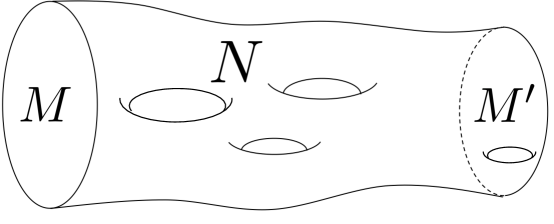
Figure 1: Bordism between manifolds. Here $M$ and $M^{\prime}$ are two closed $d$-manifolds, $N$ is a compact $d+1$-manifold whose boundary is the disjoint union of $M$ and $M^{\prime}$, so $\partial N=M\sqcup M^{\prime}$. If there are additional $G$-structures on these manifolds, then the $G$-structure on $N$ is required to be compatible with the $G$-structures on $M$ and $M^{\prime}$. If there are additional maps from these manifolds to a fixed topological space, then the maps are also required to be compatible with each other. If these conditions are satisfied, then $M$ and $M^{\prime}$ are called bordant and $N$ is called a bordism between $M$ and $M^{\prime}$. This relation is an equivalence relation.

We assume that the readers are familiar with the basic algebraic topology, such as (co)homology and homotopy. To fill in the gap between this knowledge and the mathematical tools used in this article, we introduce some prerequisites in this subsection.

First, we introduce the notion of bordism group. To define the bordism group, we need to define a tangential structure which involves the notion of classifying spaces. For any Lie group $G$, the $\mathrm{B}G$ is the classifying space of principal $G$-bundles, namely the homotopy classes of maps $X\to\mathrm{B}G$ are in one-to-one correspondence with the isomorphism classes of principal $G$-bundles over $X$ for any topological space $X$. For any abelian group $G$, the iterated classifying space $\mathrm{B}^{2}G$ is also the Eilenberg-MacLane space $K(G,2)$. For any abelian group $G$, more generally, we have the $\mathrm{B}^{d}G=K(G,d)$.

To define tangential structure, we require the orthogonal group ${\rm O}(n)$ since a tangential structure involves a fibration over the classifying space of ${\rm O}(n)$. There is a natural inclusion ${\rm O}(n)\to{\rm O}(n+1)$. Let ${\rm O}$ denote the colimit ${\rm O}:=\text{colim}_{n\to\infty}{\rm O}(n)$. The inclusions ${\mathbb{R}}^{q}\to{\mathbb{R}}^{q+1}$ induce the closed inclusions of Grassmannian spaces $Gr_{n}({\mathbb{R}}^{q})\to Gr_{n}({\mathbb{R}}^{q+1})$. The colimit $\text{colim}_{q\to\infty}Gr_{n}({\mathbb{R}}^{q})$ is the classifying space $\mathrm{B}{\rm O}(n)$. There are closed inclusions $Gr_{n}({\mathbb{R}}^{q})\to Gr_{n+1}({\mathbb{R}}^{q+1})$ obtained by sending $W\mapsto{\mathbb{R}}\oplus W$ where we write ${\mathbb{R}}^{q+1}={\mathbb{R}}\oplus{\mathbb{R}}^{q}$. These induce maps $\mathrm{B}{\rm O}(n)\to\mathrm{B}{\rm O}(n+1)$, and we define

$$\mathrm{B}{\rm O}:=\text{colim}_{n\to\infty}\mathrm{B}{\rm O}(n).$$ (1.14)

The $\mathrm{B}{\rm O}$ is a classifying space for the infinite orthogonal group ${\rm O}$.

An $n$-dimensional tangential structure is a topological space $\mathrm{B}G(n)$ and a fibration $\pi(n):\mathrm{B}G(n)\to\mathrm{B}{\rm O}(n)$. A stable tangential structure is a topological space $\mathrm{B}G$ and a fibration $\pi:\mathrm{B}G\to\mathrm{B}{\rm O}$. It gives rise to an $n$-dimensional tangential structure for each $n\in\mathbb{Z}^{\geq 0}$ by letting $\pi(n):\mathrm{B}G(n)\to\mathrm{B}{\rm O}(n)$ be the fiber product (also called pullback)

(1.19)

Here the map $\mathrm{B}{\rm O}(n)\to\mathrm{B}{\rm O}$ is the inclusion map. If $M$ is an $m$-dimensional manifold, then a $G(n)$-structure on $M$ is a lift $M\to\mathrm{B}G(n)$ of a classifying map $M\to\mathrm{B}{\rm O}(n)$ of $\widetilde{TM}$, where we have stabilized the tangent bundle $TM$ of the $m$-dimensional manifold $M$ to the rank $n$ bundle

$$\widetilde{TM}:=\underline{{\mathbb{R}}^{n-m}}\oplus TM.$$ (1.20)

Here $\underline{{\mathbb{R}}^{n-m}}$ is the trivial real vector bundle of dimension $n-m$. A $G$-structure on $M$ is a family of coherent $G(n)$-structures for $n$ sufficiently large. Here coherent $G(n)$-structures for $n$ sufficiently large means that the composite of the $G(l)$-structure on $M$ and the inclusion map $\mathrm{B}G(l)\to\mathrm{B}G(n)$: $M\to\mathrm{B}G(l)\to\mathrm{B}G(n)$ is exactly the $G(n)$-structure on $M$ for $l<n$ where $l$ and $n$ are sufficiently large. Notice that an $n$-dimensional tangential structure induces an $l$-dimensional tangential structure for all $l<n$ by taking the fiber product (also called pullback)

(1.25)

See [69] for more details.

For any structure group $G$ and any topological space $X$, we define the bordism group as the set of equivalence classes:

$$\Omega_{d}^{G}(X):=\{(M,f)\mid M\text{ is a closed }d\text{-manifold with a }G\text{-structure, }f:M\to X\text{ is a map}\}/\sim.$$ (1.26)

The $(M,f)$ is a pair of data of the manifold $M$ and map $f$. The $\sim$ is an equivalence relation defined on the set of pairs of a manifold $M$ and a map $f$. $(M,f)\sim(M^{\prime},f^{\prime})$ if and only if there is a compact $(d+1)$-manifold $N$ with a $G$-structure and a map $F:N\to X$ such that the boundary of $N$ is the disjoint union of $M$ and $M^{\prime}$ (Figure 1), the $G$-structures on $M$ and $M^{\prime}$ are induced from the $G$-structure on $N$, and $F|_{M}=f$ and $F|_{M^{\prime}}=f^{\prime}$. The disjoint union operation on closed $d$-manifolds induces an abelian group structure on $\Omega_{d}^{G}(X)$. Here a $G$-structure on a manifold is a $G$-structure on the stable tangent bundle of this manifold. In this article, we will focus on the case when $X$ is a classifying space. In most cases, $X$ is just a point.

If $\Omega_{d}^{G}(X)=G_{1}\times G_{2}\times\cdots\times G_{r}$ where $G_{i}$ are cyclic groups, then the group homomorphisms $\varphi_{i}:\Omega_{d}^{G}(X)\to G_{i}$ are called bordism invariants, and they form a complete set of bordism invariants if $\varphi=(\varphi_{1},\varphi_{2},\dots,\varphi_{r}):\Omega_{d}^{G}(X)\to G_{1}\times G_{2}\times\cdots\times G_{r}$ is a group isomorphism. So $(M,f)$ and $(M^{\prime},f^{\prime})$ are in the same equivalence class of the bordism group $\Omega_{d}^{G}(X)$ if and only if the values of each bordism invariant $\varphi_{i}$ on $(M,f)$ and $(M^{\prime},f^{\prime})$ are the same for $1\leq i\leq r$.

In this article, we will compute the bordism groups $\Omega_{d}^{G}$ for $G={\rm Spin}\times G^{\prime}$ or ${\rm Spin}\times_{\mathbb{Z}_{2}}G^{\prime}$ for some groups $G^{\prime}$. So we first clarify these notations here. ${\rm Spin}$ (or ${\rm Spin}(d)$) is a nontrivial extension of the group ${\rm SO}$ (or ${\rm SO}(d)$) by $\mathbb{Z}_{2}$, namely there are short exact sequences of groups

$$1\to\mathbb{Z}_{2}\to{\rm Spin}\to{\rm SO}\to 1,$$ (1.27)

$$1\to\mathbb{Z}_{2}\to{\rm Spin}(d)\to{\rm SO}(d)\to 1,$$ (1.28)

where ${\rm SO}$ is the colimit of ${\rm SO}(d)$, and ${\rm SO}(d)$ is the special orthogonal group. The ${\rm Spin}$ is the colimit of ${\rm Spin}(d)$. The ${\rm Spin}\times_{\mathbb{Z}_{2}}G^{\prime}$ is the quotient group of ${\rm Spin}\times G^{\prime}$ by the diagonal central subgroup $\mathbb{Z}_{2}$.

1.2.2 Spectra

For a pointed topological space $X$, the $\Sigma$ denotes a suspension $\Sigma X=S^{1}\wedge X=(S^{1}\times X)/(S^{1}\vee X)$ where $\wedge$ and $\vee$ are smash product and wedge sum (a one point union) of pointed topological spaces respectively.

Now we recall some basic notions regarding spectrum, see [69, 31] for more details. A prespectrum $T_{\bullet}$ is a sequence $\{T_{n}\}_{n\in\mathbb{Z}^{\geq 0}}$ of pointed spaces and the maps $s_{n}:\Sigma T_{n}\to T_{n+1}$. An $\Omega$-prespectrum is a prespectrum $T_{\bullet}$ such that the adjoints $t_{q}:T_{n}\to\Omega T_{n+1}$ of the structure maps are weak homotopy equivalences. Here $\Omega$ means the loop space, its meaning is different from the bordism notation $\Omega$. A spectrum is a prespectrum $T_{\bullet}$ such that the adjoints $t_{n}:T_{n}\to\Omega T_{n+1}$ of the structure maps are homeomorphisms. For example, let $X$ be a pointed space, $T_{n}=\Sigma^{n}X$ for $n\geq 0$, then $T_{\bullet}$ is a prespectrum. In particular, if $T_{n}=S^{n}$, then $T_{\bullet}$ is a prespectrum. Let $G$ be an abelian group, $T_{n}=K(G,n)$ be the Eilenberg-MacLane space, then $T_{\bullet}$ is an $\Omega$-prespectrum. In general, these examples are not spectra. But we can always construct a spectrum from a prespectrum using spectrification.

Let $T_{\bullet}$ be a prespectrum, define $(LT)_{n}$ to be the colimit of

$$T_{n}\xrightarrow{t_{n}}\Omega T_{n+1}\xrightarrow{\Omega t_{n+1}}\Omega^{2}T_{n+2}\xrightarrow{\Omega^{2}t_{n+2}}\dots\xrightarrow{\Omega^{l-1}t_{n+l-1}}\Omega^{l}T_{n+l}\xrightarrow{\Omega^{l}t_{n+l}}\dots.$$

Namely,

$$(LT)_{n}=\text{colim}_{l\to\infty}\Omega^{l}T_{n+l},$$

then $(LT)_{\bullet}$ is a spectrum, called the spectrification of $T_{\bullet}$. For example, if $T_{n}=S^{n}$, then $(LT)_{\bullet}$ is a spectrum $\mathbb{S}$ (the sphere spectrum). Let $G$ be an abelian group, $T_{q}=K(G,n)$ the Eilenberg-MacLane space, then $(LT)_{\bullet}$ is a spectrum $HG$ (the Eilenberg-MacLane spectrum).

Next we define the homotopy groups and cohomology rings of prespectra. Let $T_{\bullet}$ be a prespectrum, we define the (stable) homotopy group $\pi_{d}T_{\bullet}$ to be the colimit of

$$\pi_{d+n}T_{n}\xrightarrow{\pi_{d+n}t_{n}}\pi_{d+n}\Omega T_{n+1}\xrightarrow{\text{adjunction}}\pi_{d+n+1}T_{n+1}\dots.$$

Namely,

$$\pi_{d}T_{\bullet}=\text{colim}_{n\to\infty}\pi_{d+n}T_{n}.$$

If $\rm{M}_{\bullet}$ and $\rm{N}_{\bullet}$ are two prespectra, and $\rm{N}_{\bullet}$ is an $\Omega$-prespectrum, then for any integer $k$, the abelian group of homotopy classes of maps from $\rm{M}_{\bullet}$ to $\rm{N}_{\bullet}$ of degree $-k$ is defined as follows: a map from $\rm{M}_{\bullet}$ to $\rm{N}_{\bullet}$ of degree $-k$ is a sequence of maps $\rm{M}_{n}\to\rm{N}_{n+k}$ such that the following diagram commutes

(1.33)

where the columns are the structure maps of the prespectra $\rm{M}_{\bullet}$ and $\rm{N}_{\bullet}$. Two maps of prespectra of degree $-k$: $f,g:\rm{M}_{\bullet}\to\rm{N}_{\bullet+k}$ are homotopic, denoted $f\simeq g$, if there is a map $H:\rm{M}_{\bullet}\wedge I_{+}\to\rm{N}_{\bullet+k}$ which restricts to $f\vee g$ along the inclusion $\rm{M}_{\bullet}\vee\rm{M}_{\bullet}\xrightarrow{i_{0}\vee i_{1}}\rm{M}_{\bullet}\wedge I_{+}\xrightarrow{H}\rm{N}_{\bullet+k}$ where the interval $I=[0,1]$, $I_{+}$ is the disjoint union of $I$ and a base point. Here $i_{0}$ and $i_{1}$ are the inclusion maps at $0\in I$ and $1\in I$ respectively. Note that $\Sigma(\rm{M}_{\bullet}\times I)\neq\Sigma\rm{M}_{\bullet}\times I$, so we use $\rm{M}\wedge I_{+}$ instead of $\rm{M}_{\bullet}\times I$. The $[\rm{M}_{\bullet},\rm{N}_{\bullet}]_{-k}$ is an abelian group since $\rm{N}_{\bullet}$ is an $\Omega$-prespectrum. If in addition, $\rm{N}_{\bullet}$ is a ring spectrum, then the abelian groups $[\rm{M}_{\bullet},\rm{N}_{\bullet}]_{-k}$ form a graded ring $[\rm{M}_{\bullet},\rm{N}_{\bullet}]_{-*}$. In particular, $[\rm{M}_{\bullet},\rm{N}_{\bullet}]:=[\rm{M}_{\bullet},\rm{N}_{\bullet}]_{0}$. For example, $\pi_{d}\rm{M}_{\bullet}=[\mathbb{S},\rm{M}_{\bullet}]_{d}$. Let $R$ be a ring, then the Eilenberg-MacLane spectrum $HR$ is a ring spectrum. The cohomology ring of a prespectrum $\rm{M}_{\bullet}$ with coefficients in $R$ is defined to be $\operatorname{H}^{*}(\rm{M}_{\bullet},R):=[\rm{M}_{\bullet},HR]_{-*}$.

Let $V\to Y$ be a real vector bundle, and fix a Euclidean metric. The Thom space $\text{Thom}(Y;V)$ is the quotient $D(V)/S(V)$ where $D(V)$ is the unit disk bundle and $S(V)$ is the unit sphere bundle. Namely, $D(V)=\{v\in V\mid|v|\leq 1\}$ and $S(V)=\{v\in V\mid|v|=1\}$ where $|\cdot|$ denotes the Euclidean norm.

Thom spaces satisfy

$$\text{Thom}(X\times Y;V\times W) = \text{Thom}(X;V)\wedge\text{Thom}(Y;W),$$

$$\text{Thom}(X;V\oplus\underline{{\mathbb{R}}^{n}}) = \Sigma^{n}\text{Thom}(X;V),$$

$$\text{Thom}(X;\underline{{\mathbb{R}}^{n}}) = \Sigma^{n}X_{+},$$ (1.34)

where $V\to X$ and $W\to Y$ are real vector bundles, $\underline{{\mathbb{R}}^{n}}$ is the trivial real vector bundle of dimension $n$, and $X_{+}$ is the disjoint union of $X$ and a point.

Let $G$ be a group with a group homomorphism $\rho:G\to{\rm O}$. Let $MG(n)=\text{Thom}(\mathrm{B}G(n);V_{n})$, where $V_{n}$ is the induced vector bundle (of dimension $n$) by the map $\mathrm{B}G(n)\to\mathrm{B}{\rm O}(n)$. Let $T_{n}=MG(n)$, then $T_{\bullet}$ is a prespectrum by the property of Thom spaces. The Thom spectrum $MG$ is the spectrification of $T_{\bullet}$. In other words, $MG=\text{Thom}(\mathrm{B}G;V)$ where $V$ is the colimit of $V_{n}-n$.

Let $G$ be a group with a group homomorphism $\rho:G\to{\rm O}$. The Madsen-Tillmann spectrum $MTG$ is the colimit of $\Sigma^{n}MTG(n)$, where the virtual Thom spectrum $MTG(n)=\text{Thom}(\mathrm{B}G(n);-V_{n})$ is the spectrification of the prespectrum whose $(n+q)$-th space is $\text{Thom}(\mathrm{B}G(n,n+q);Q_{q})$ where $\mathrm{B}G(n,n+q)$ is the pullback

(1.39)

and there is a direct sum $\underline{{\mathbb{R}}^{n+q}}=V_{n}\oplus Q_{q}$ of vector bundles over $Gr_{n}({\mathbb{R}}^{n+q})$ and, by pullback, over $\mathrm{B}G(n,n+q)$ where $\underline{{\mathbb{R}}^{n+q}}$ is the trivial real vector bundle of dimension $n+q$. In other words, $MTG=\text{Thom}(\mathrm{B}G;-V)$ where $V$ is the colimit of $V_{n}-n$.

1.2.3 Adams spectral sequence

Adams spectral sequence is a mathematical tool to compute the homotopy groups of spectra [70]. In particular, the homotopy group of the Madsen-Tillmann spectrum $MTG$ [39] is the bordism group $\Omega_{d}^{G}$. We use Adams spectral sequence to compute several bordism groups related to Standard Models (SM), Grand Unified Theories (GUT) and beyond. We also compute the group $\mathrm{TP}_{d}(G)$ classifying the topological phases (i.e., the topological terms in QFT or the topological phases of quantum matter) based on the computation of bordism groups and a short exact sequence. See [19, 35, 31] for primers. We will call the group $\mathrm{TP}_{d}(G)$ the cobordism group. The relation between $\Omega_{d}^{G}$ and $\mathrm{TP}_{d}(G)$ is like that between homology group and cohomology group, as we will see later.

The Adams spectral sequence shows [70]:

$$\operatorname{Ext}_{\mathcal{A}_{p}}^{s,t}(\operatorname{H}^{*}(Y,\mathbb{Z}_{p}),\mathbb{Z}_{p})\Rightarrow(\pi_{t-s}(Y))_{p}^{\wedge},$$ (1.40)

where the Ext denotes the extension functor. Note that this extension functor has 2 upper indices. It is different from but similar to the usual extension functor. The index $s$ refers to the degree of resolution, and the index $t$ is the internal degree of the graded module. Here $\mathcal{A}_{p}=[H\mathbb{Z}_{p},H\mathbb{Z}_{p}]_{-*}$ is the mod $p$ Steenrod algebra which consists of mod $p$ cohomology operations [71], and $Y$ is any spectrum. In particular, the mod 2 Steenrod algebra $\mathcal{A}_{2}$ is generated by the Steenrod squares $\mathrm{Sq}^{i}:\operatorname{H}^{*}(-,\mathbb{Z}_{2})\to\operatorname{H}^{*+i}(-,\mathbb{Z}_{2})$. By the Yoneda lemma, the $\operatorname{H}^{*}(Y,\mathbb{Z}_{p})=[Y,H\mathbb{Z}_{p}]_{-*}$ is automatically an $\mathcal{A}_{p}$-module whose internal degree $t$ is given by the $*$. The $(\pi_{t-s}(Y))_{p}^{\wedge}$ is the $p$-completion of the $(t-s)$-th homotopy group of the spectrum $Y$. For any finitely generated abelian group ${\cal G}$, the abelian group ${\cal G}_{p}^{\wedge}=\lim_{n\to\infty}{\cal G}/p^{n}{\cal G}$ is the $p$-completion of ${\cal G}$. We note that, if ${\cal G}$ is a finite abelian group, then the ${\cal G}_{p}^{\wedge}$ is the Sylow $p$-subgroup of ${\cal G}$; if ${\cal G}$ is the infinite cyclic group $\mathbb{Z}$, then the ${\cal G}_{p}^{\wedge}$ is the ring of $p$-adic integers. Here the ${\cal G}$ is meant to be substituted by a homotopy group $\pi_{t-s}(Y)$ in (1.40). Here are some explanations and inputs:

1. Here the double-arrow “$\Rightarrow$” means “convergent to.” The $E_{2}$ page are groups $\operatorname{Ext}^{s,t}$ with double indices $(s,t)$, we reindex the bidegree by $(t-s,s)$. Inductively, there are differentials $d_{r}$ in $E_{r}$ page which are arrows from $(t-s,s)$ to $(t-s-1,s+r)$ (that is, $\operatorname{Ext}^{s,t}\to\operatorname{Ext}^{s+r,t+r-1}$). Take Ker$d_{r}$/Im$d_{r}$ at each $(t-s,s)$, then we get the $E_{r+1}$ page. Finally $E_{r}$ page equals $E_{r+1}$ page (there are no differentials) for $r\geq N$, we call this $E_{N}$ page as the $E_{\infty}$ page, we can read the result $\pi_{d}$ at $t-s=d$. See further details discussed in LABEL:WanWang2018bns1812.11967’s Sec. 2.3.

   Figure 2: The $E_{r}$ page of Adams spectral sequence

2. In Adams spectral sequence, we consider $\operatorname{Ext}_{R}^{s,t}(L,\mathbb{Z}_{p})$. In this article, we will consider the algebra $R=\mathcal{A}_{p}$ or $\mathcal{A}_{2}(1)$ for $p=2$, and $L$ is an $R$-module. The $\mathcal{A}_{2}(1)$ is the subalgebra of $\mathcal{A}_{2}$ generated by the Steenrod squares $\mathrm{Sq}^{1}$ and $\mathrm{Sq}^{2}$. Ext groups are defined by firstly taking a projective $R$-resolution $P_{\bullet}$ of $L$, then secondly computing the (co)homology group of the (co)chain complex $\operatorname{Hom}(P_{\bullet},\mathbb{Z}_{p})$. Here a projective $R$-resolution $P_{\bullet}$ is an exact sequence of $R$-modules $\cdots\to P_{s}\to P_{s-1}\to\cdots\to P_{0}\to L$ where $P_{s}$ is a projective $R$-module for $s\geq 0$. An $R$-module is projective if and only if it is a direct summand of a free $R$-module.

For $Y=MTG$, where $MTG$ is the Madsen-Tillmann spectrum of a group $G$, the Adams spectral sequence (1.40) shows:

$$\operatorname{Ext}_{\mathcal{A}_{p}}^{s,t}(\operatorname{H}^{*}(MTG,\mathbb{Z}_{p}),\mathbb{Z}_{p})\Rightarrow\pi_{t-s}(MTG)_{p}^{\wedge}=(\Omega_{d=t-s}^{G})_{p}^{\wedge}.$$ (1.41)

The last equality is by the generalized Pontryagin-Thom isomorphism, we have an equality between the $d$-th bordism group of $G$ given by $\Omega_{d}^{G}$ and the $d$-th homotopy group of $MTG$ given by $\pi_{d}(MTG)$, namely

$$\Omega_{d}^{G}=\pi_{d}(MTG).$$ (1.42)

The $T$ in $MTG$ means that the $G$-structures are on the stable tangent bundles instead of stable normal bundles. For Spin, the Madsen-Tillmann spectrum $MT{\rm Spin}=M{\rm Spin}$ is equivalent to the Thom spectrum.

We also compute the cobordism group of topological phases (TP) defined in [19] as

$$\mathrm{TP}_{d}(G):=[MTG,\Sigma^{d+1}I\mathbb{Z}].$$ (1.43)

Here $I\mathbb{Z}$ is the Anderson dual spectrum. By [19], the torsion part of $\mathrm{TP}_{d}(G)$ classifies deformation classes of reflection positive invertible $d$-dimensional extended topological field theories with a symmetry group $G(d)$. Here $G(d)$ means the $d$-dimensional spacetime version of the group $G$. The $\mathrm{TP}_{d}(G)$ and the bordism group $\Omega_{d}^{G}$ are related by a short exact sequence

$$0\to\operatorname{Ext}^{1}(\Omega_{d}^{G},\mathbb{Z})\to\mathrm{TP}_{d}(G)\to\operatorname{Hom}(\Omega_{d+1}^{G},\mathbb{Z})\to 0.$$ (1.44)

This short exact sequence is very similar to the universal coefficient theorem relating homology group and cohomology group. It is split, since $\operatorname{Ext}^{1}(\Omega_{d}^{G},\mathbb{Z})$ is always torsion, $\operatorname{Hom}(\Omega_{d+1}^{G},\mathbb{Z})$ is always free, and $\operatorname{Ext}^{1}(\mathbb{Z},\mathbb{Z}_{n})=0$. So we can directly derive the group $\mathrm{TP}_{d}(G)$ from the data of $\Omega_{d}^{G}$ and $\Omega_{d+1}^{G}$.

We will use the (1.41) and (1.42) to compute the $d$-th bordism group of $G$ given by $\Omega_{d}^{G}$. Then we will use (1.44) to compute the $d$-th cobordism group of topological phases of $G$ given by $\mathrm{TP}_{d}(G)$.

If $G={\rm Spin}\times G^{\prime}$, then $\mathrm{B}G=\mathrm{B}{\rm Spin}\times\mathrm{B}G^{\prime}$. By definition, the Madsen-Tillmann spectrum $MTG=\text{Thom}(\mathrm{B}G;-V)$ where $V$ is the induced virtual bundle of dimension 0 by the map $\mathrm{B}G\to\mathrm{B}{\rm O}$. By the properties of Thom space (1.2.2), we have

$$MT({\rm Spin}\times G^{\prime})=M{\rm Spin}\wedge(\mathrm{B}G^{\prime})_{+}.$$ (1.45)

The $\wedge$ is the smash product. The $(\mathrm{B}G^{\prime})_{+}$ is the disjoint union of the classifying space $\mathrm{B}G^{\prime}$ and a point. By the generalized Pontryagin-Thom isomorphism, for any structure group $G$ and any topological space $X$, we have

$$\Omega_{d}^{G}(X)=\pi_{d}(MTG\wedge X_{+}).$$ (1.46)

Since $MT{\rm Spin}=M{\rm Spin}$, we have

$$\Omega_{d}^{{\rm Spin}\times G^{\prime}}=\pi_{d}(MT({\rm Spin}\times G^{\prime}))=\pi_{d}(M{\rm Spin}\wedge(\mathrm{B}G^{\prime})_{+})=\Omega_{d}^{{\rm Spin}}(\mathrm{B}G^{\prime}).$$ (1.47)

If $MTG=M{\rm Spin}\wedge X$ where $X$ is any topological space, by Corollary 5.1.2 of [72] which is based on [73], we have

$$\operatorname{Ext}_{\mathcal{A}_{2}}^{s,t}(\operatorname{H}^{*}(M{\rm Spin}\wedge X,\mathbb{Z}_{2}),\mathbb{Z}_{2})=\operatorname{Ext}_{\mathcal{A}_{2}(1)}^{s,t}(\operatorname{H}^{*}(X,\mathbb{Z}_{2}),\mathbb{Z}_{2})$$ (1.48)

for $t-s<8$. Here $\mathcal{A}_{2}(1)$ is the subalgebra of $\mathcal{A}_{2}$ generated by $\mathrm{Sq}^{1}$ and $\mathrm{Sq}^{2}$.

So for the dimension $d=t-s<8$, we have

$$\operatorname{Ext}_{\mathcal{A}_{2}(1)}^{s,t}(\operatorname{H}^{*}(X,\mathbb{Z}_{2}),\mathbb{Z}_{2})\Rightarrow(\Omega_{t-s}^{G})_{2}^{\wedge}.$$ (1.49)

The reduced cohomology $\operatorname{H}^{*}(X,\mathbb{Z}_{2})$ is an $\mathcal{A}_{2}(1)$-module whose internal degree $t$ is given by the $*$.

Lemma 1 (Lemma 11 of [31]).

Given a short exact sequence of $\mathcal{A}_{2}(1)$-modules

$$0\to L_{1}\to L_{2}\to L_{3}\to 0,$$ (1.50)

then for any $t$, there is a long exact sequence

$$\cdots\to\operatorname{Ext}_{\mathcal{A}_{2}(1)}^{s,t}(L_{3},\mathbb{Z}_{2})\to\operatorname{Ext}_{\mathcal{A}_{2}(1)}^{s,t}(L_{2},\mathbb{Z}_{2})\to\operatorname{Ext}_{\mathcal{A}_{2}(1)}^{s,t}(L_{1},\mathbb{Z}_{2})$$ (1.51)

$$\stackrel{{\scriptstyle d_{1}}}{{\to}}\operatorname{Ext}_{\mathcal{A}_{2}(1)}^{s+1,t}(L_{3},\mathbb{Z}_{2})\to\operatorname{Ext}_{\mathcal{A}_{2}(1)}^{s+1,t}(L_{2},\mathbb{Z}_{2})\to\cdots$$

We can compute the $E_{2}$ page of $\mathcal{A}_{2}(1)$-module based on Lemma 1. More precisely, in order to compute $\operatorname{Ext}_{\mathcal{A}_{2}(1)}^{s,t}(L_{2},\mathbb{Z}_{2})$, we find a short exact sequence of $\mathcal{A}_{2}(1)$-modules

$$0\to L_{1}\to L_{2}\to L_{3}\to 0,$$ (1.52)

then we apply Lemma 1 to compute $\operatorname{Ext}_{\mathcal{A}_{2}(1)}^{s,t}(L_{2},\mathbb{Z}_{2})$ by the given data of $\operatorname{Ext}_{\mathcal{A}_{2}(1)}^{s,t}(L_{1},\mathbb{Z}_{2})$ and $\operatorname{Ext}_{\mathcal{A}_{2}(1)}^{s,t}(L_{3},\mathbb{Z}_{2})$. Our strategy is choosing $L_{1}$ to be the direct sum of suspensions of $\mathbb{Z}_{2}$ on which $\mathrm{Sq}^{1}$ and $\mathrm{Sq}^{2}$ act trivially, then we take $L_{3}$ to be the quotient of $L_{2}$ by $L_{1}$. If $\operatorname{Ext}_{\mathcal{A}_{2}(1)}^{s,t}(L_{3},\mathbb{Z}_{2})$ is undetermined, then we take $L_{3}$ to be the new $L_{2}$ and repeat this procedure. We can use this procedure again and again until $\operatorname{Ext}_{\mathcal{A}_{2}(1)}^{s,t}(L_{2},\mathbb{Z}_{2})$ is determined.

1.2.4 Characteristic classes

Throughout the article, we use the standard notation for characteristic classes: $w_{i}$ for the Stiefel-Whitney class, $c_{i}$ for the Chern class, $p_{i}$ for the Pontryagin class, and $e_{n}$ for the Euler class. Note that the Euler class only appears in the total dimension of the vector bundle. We use the notation $w_{i}(G)$, $c_{i}(G)$, $p_{i}(G)$, and $e_{n}(G)$ to denote the characteristic classes of the associated vector bundle of the principal $G$ bundle (normally denoted as $w_{i}(V_{G})$, $c_{i}(V_{G})$, $p_{i}(V_{G})$, and $e_{n}(V_{G})$). For simplicity, we may denote the Stiefel-Whitney class of the tangent bundle $TM$ as $w_{j}\equiv w_{j}(TM)$; if we do not specify $w_{j}$ with which bundle, then we really mean $TM$.

We will use $\text{CS}_{2n-1}^{V}$ to denote the Chern-Simons $2n-1$-form for the Chern class (if $V$ is a complex vector bundle) or the Pontryagin class (if $V$ is a real vector bundle). Note that $p_{i}(V)=(-1)^{i}c_{2i}(V\otimes{\mathbb{C}})$. The relation between the Chern-Simons form and the Chern class is

$$c_{n}(V)=\hskip 1.0pt\mathrm{d}\text{CS}_{2n-1}^{V}$$ (1.53)

where the $\hskip 1.0pt\mathrm{d}$ is the exterior differential and the $c_{n}(V)$ is regarded as a closed differential form in de Rham cohomology.

There is also another kind of Chern-Simons form for Euler class $e_{2n}(V)$ [74], we denote it by $\text{CS}_{2n-1,e}^{V}$, it satisfies

$$e_{2n}(V)=\hskip 1.0pt\mathrm{d}\text{CS}_{2n-1,e}^{V}.$$ (1.54)

The relations between Pontryagin class, Euler class and Stiefel-Whitney class are

$$p_{i}(V)=w_{2i}(V)^{2}\mod 2$$ (1.55)

and

$$e_{2n}(V)=w_{2n}(V)\mod 2$$ (1.56)

where $2n=\dim V$.

By the Hirzebruch signature theorem, the relation between the signature and the first Pontryagin class of a 4-manifold $M$ is

$$\sigma=\frac{1}{3}\int_{M}p_{1}(TM).$$ (1.57)

1.3 Lie algebra to Lie group and the representation theory

To justify the spacetime symmetry group $G_{\text{spacetime}}$ and internal symmetry group $G_{\text{internal}}$ relevant for Standard Model physics, we shall first review the Lie algebra of Standard Models, to the representation theory of matter field contents, and to the Lie groups of Standard Models.

1. The local gauge structure of Standard Model is given by the Lie algebra $u(1)\times su(2)\times su(3)$. This means that the Lie algebra valued 1-form gauge fields take values in $u(1)\times su(2)\times su(3)$. The 1-form gauge fields are the 1-connections of the principals $G_{\text{internal}}$-bundles that we should determine.

2. Fermions as the spinor fields. A spinor field is a section of the spinor bundle. For the left-handed Weyl spinor $\Psi_{L}$, it is a doublet spin-1/2 representation of spacetime symmetry group $G_{\text{spacetime}}$ (Minkowski ${\rm Spin}(3,1)$ or Euclidean ${\rm Spin}(4)$), denoted as

   $$\Psi_{L}\sim{\bf 2}_{L}\text{ of }{\rm Spin}(3,1),\text{ or }\Psi_{L}\sim{\bf 2}_{L}\text{ of }{\rm Spin}(4).$$ (1.58)

   On the other hand, the matter fields as Weyl spinors $\Psi_{L}$ contain:

   • The left-handed up and down quarks ($u$ and $d$) form a doublet $\begin{pmatrix}u\\ d\end{pmatrix}_{L}$ in ${\bf 2}$ for the SU(2)${}_{\text{weak}}$, and they are in ${\bf 3}$ for the SU(3)${}_{\text{strong}}$.

   • The right-handed up and down quarks, each forms a singlet $u_{R}$ and $d_{R}$ in ${\bf 1}$ for the SU(2)${}_{\text{weak}}$. They are in ${\bf 3}$ for the SU(3)${}_{\text{strong}}$.

   • The left-handed electron and neutrino form a doublet $\begin{pmatrix}\nu_{e}\\ e\end{pmatrix}_{L}$ in ${\bf 2}$ for the SU(2)${}_{\text{weak}}$, and they are in ${\bf 1}$ for the SU(3)${}_{\text{strong}}$.

   • The right-handed electron forms a singlet in ${\bf 1}$ for the SU(2)${}_{\text{weak}}$, and it is in ${\bf 1}$ for the SU(3)${}_{\text{strong}}$.

   There are two more families of quarks: charm and strange quarks ($c$ and $s$), and top and bottom quarks ($t$ and $b$). There are also two more families of leptons: muon and its neutrino ($\mu$ and $\nu_{\mu}$), and tauon and its neutrino ($\tau$ and $\nu_{\tau}$). So there are three families (i.e., generations) of quarks and leptons:

   $$\Bigg{(}\begin{pmatrix}u\\ d\end{pmatrix}_{L}\times{\bf 3}_{\text{color}},\quad\quad\quad u_{R}\times{\bf 3}_{\text{color}},\quad\quad\quad\quad d_{R}\times{\bf 3}_{\text{color}},\quad\quad\quad\begin{pmatrix}\nu_{e}\\ e\end{pmatrix}_{L},\quad\quad\quad e_{R}\quad\Bigg{)},$$ (1.59)

   $$\Bigg{(}\begin{pmatrix}c\\ s\end{pmatrix}_{L}\times{\bf 3}_{\text{color}},\quad\quad\quad c_{R}\times{\bf 3}_{\text{color}},\quad\quad\quad\quad s_{R}\times{\bf 3}_{\text{color}},\quad\quad\quad\begin{pmatrix}\nu_{\mu}\\ \mu\end{pmatrix}_{L},\quad\quad\quad\mu_{R}\quad\Bigg{)},$$ (1.60)

   $$\Bigg{(}\begin{pmatrix}t\\ b\end{pmatrix}_{L}\times{\bf 3}_{\text{color}},\quad\quad\quad t_{R}\times{\bf 3}_{\text{color}},\quad\quad\quad\quad b_{R}\times{\bf 3}_{\text{color}},\quad\quad\quad\begin{pmatrix}\nu_{\tau}\\ \tau\end{pmatrix}_{L},\quad\quad\quad\tau_{R}\quad\Bigg{)}.$$ (1.61)

   In short, for all of them as three families, we can denote them as:

   $$\Bigg{(}\begin{pmatrix}u\\ d\end{pmatrix}_{L}\times{\bf 3}_{\text{color}},\quad\quad\quad u_{R}\times{\bf 3}_{\text{color}},\quad\quad\quad\quad d_{R}\times{\bf 3}_{\text{color}},\quad\quad\quad\begin{pmatrix}\nu_{e}\\ e\end{pmatrix}_{L},\quad\quad\quad e_{R}\quad\Bigg{)}\times\text{3 families}.$$ (1.62)

   In fact, all the following four kinds of

   $$G_{\text{internal}}=\frac{{\rm SU}(3)\times{\rm SU}(2)\times{\rm U}(1)}{\mathbb{Z}_{q}}$$ (1.63)

   with $q=1,2,3,6$ are compatible with the above representations of fermion fields. These Weyl spinors can be written in the following more succinct forms of representations for any of the internal symmetry group $G_{\text{internal}}$ with $q=1,2,3,6$:

   $$\Bigg{(}({\bf 3},{\bf 2},1/6)_{L},({\bf 3},{\bf 1},2/3)_{R},({\bf 3},{\bf 1},-1/3)_{R},({\bf 1},{\bf 2},-1/2)_{L},({\bf 1},{\bf 1},-1)_{R}\Bigg{)}\times\text{3 families}$$

   $$\Rightarrow\Bigg{(}({\bf 3},{\bf 2},1/6)_{L},(\overline{\bf 3},{\bf 1},-2/3)_{L},(\overline{\bf 3},{\bf 1},1/3)_{L},({\bf 1},{\bf 2},-1/2)_{L},({\bf 1},{\bf 1},1)_{L}\Bigg{)}\times\text{3 families}.$$ (1.64)

   The triplet given above is listed by their (SU(3) representation, SU(2) representation, hypercharge $Y$). For example, $({\bf 3},{\bf 2},1/6)$ means that ${\bf 3}$ in SU(3), ${\bf 2}$ in SU(2) and 1/6 for hypercharge. In the second line, we transforms the right-handed Weyl spinor $\Psi_{R}\sim{\bf 2}_{R}\text{ of }{\rm Spin}(3,1)$ to its left-handed $\Psi_{L}\sim{\bf 2}_{L}\text{ of }{\rm Spin}(3,1)$, while we flip their (SU(3) representation, SU(2) representation, hypercharge) to its (complex) conjugation representations. If we include the right-handed neutrinos (say ${\nu_{e}}_{R}$, ${\nu_{\mu}}_{R}$, and ${\nu_{\tau}}_{R}$), they are all in the representation $({\bf 1},{\bf 1},0)_{R}$ with no hypercharge. We can also represent a right-handed neutrino by the left-handed (complex) conjugation version $({\bf 1},{\bf 1},0)_{L}$.

   Also the complex scalar Higgs field $\phi_{H}$ is in a representation $({\bf 1},{\bf 2},1/2)$. In the Higgs condensed phase, the conventional Higgs vacuum expectation value (vev) is chosen to be $\langle\phi_{H}\rangle=\frac{1}{\sqrt{2}}\begin{pmatrix}0\\ v\end{pmatrix}$, which vev has $Q_{\rm{EM}}=0$.

3. If we include the $3\times 2+3+3+2+1=15$ left-handed Weyl spinors from one single family, we can combine them as a multiplet of $\overline{\bf 5}$ and 10 left-handed Weyl spinors of SU(5):

   $$(\overline{\bf 3},{\bf 1},1/3)_{L}\oplus({\bf 1},{\bf 2},-1/2)_{L} \sim \overline{\bf 5}\text{ of }{\rm SU}(5),$$ (1.66)

   $$({\bf 3},{\bf 2},1/6)_{L}\oplus(\overline{\bf 3},{\bf 1},-2/3)_{L}\oplus({\bf 1},{\bf 1},1)_{L} \sim {\bf 10}\text{ of }{\rm SU}(5).$$ (1.67)

   Hence we can study the SU(5) GUT with a SU(5) gauge group.

4. If we include the $3\times 2+3+3+2+1=15$ left-handed Weyl spinors from one single family, and also a right-handed neutrino, we can combine them as a multiplet of 16 left-handed Weyl spinors:

   $$\quad\Psi_{L}\sim{\bf 16}^{+}\text{ of }{\rm Spin}(10),$$ (1.68)

   which sits at the 16-dimensional irreducible spinor representation of Spin(10). (There are ${\bf 16}^{+}$ and ${\bf 16}^{-}$-dimensional irreducible spinor representation together form a ${\bf 32}$-dimensional reducible spinor representation of Spin(10).) Namely, we should study the SO(10) GUT with a Spin(10) gauge group instead of a SO(10) gauge group.

5. We find the following Lie group embedding for the internal symmetry of GUTs and Standard Models:

   $${\rm SO}(10)\supset{\rm SU}(5)\supset\frac{{\rm U}(1)\times{\rm SU}(2)\times{\rm SU}(3)}{\mathbb{Z}_{6}}.$$ (1.69)

   $${\rm Spin}(10)\supset{\rm SU}(5)\supset\frac{{\rm U}(1)\times{\rm SU}(2)\times{\rm SU}(3)}{\mathbb{Z}_{6}}.$$ (1.70)

   The other ${\mathbb{Z}_{q}}$ for $q=1,2,3$ cannot be embedded into Spin(10) nor SU(5). So from the GUT perspective, it is natural to consider the Standard Model gauge group $\frac{{\rm U}(1)\times{\rm SU}(2)\times{\rm SU}(3)}{\mathbb{Z}_{6}}$.

6. We find the following group embedding for the spacetime and internal symmetries of GUTs and Standard Models (see also [34] for the derivations):

   $${\frac{{\rm Spin}(d)\times{\rm Spin}(10)}{{\mathbb{Z}_{2}^{F}}}\supset{\rm Spin}(d)\times{\rm SU}(5)\supset{\rm Spin}(d)\times\frac{{\rm SU}(3)\times{\rm SU}(2)\times{\rm U}(1)}{\mathbb{Z}_{6}}}.$$ (1.71)

   $${{{\rm Spin}(d)\times{\rm Spin}(10)}\supset{\rm Spin}(d)\times{\rm SU}(5)\supset{\rm Spin}(d)\times\frac{{\rm SU}(3)\times{\rm SU}(2)\times{\rm U}(1)}{\mathbb{Z}_{6}}}.$$ (1.72)

We shall study the cobordism theory of these SM, BSM, and GUT groups in the following subsections.

2 Standard Models

Now we consider the co/bordism classes relevant for Standard Model (SM) physics [3, 4, 5].

2.1 ${{\rm Spin}\times{{\rm SU}(3)\times{\rm SU}(2)\times{\rm U}(1)}}$ model

We consider $G={{\rm Spin}\times{{\rm SU}(3)\times{\rm SU}(2)\times{\rm U}(1)}}$, the Madsen-Tillmann spectrum $MTG$ of the group $G$ is

$$MTG=M{\rm Spin}\wedge(\mathrm{B}({\rm SU}(3)\times{\rm SU}(2)\times{\rm U}(1)))_{+}.$$ (2.1)

The $(\mathrm{B}({\rm SU}(3)\times{\rm SU}(2)\times{\rm U}(1)))_{+}$ is the disjoint union of the classifying space $\mathrm{B}({\rm SU}(3)\times{\rm SU}(2)\times{\rm U}(1))$ and a point, see footnote 17.

For the dimension $d=t-s<8$, since there is no odd torsion, for $MTG=M{\rm Spin}\wedge(\mathrm{B}({\rm SU}(3)\times{\rm SU}(2)\times{\rm U}(1)))_{+}$, for the dimension $d=t-s<8$, by (1.49), we have the Adams spectral sequence

$$\operatorname{Ext}_{\mathcal{A}_{2}(1)}^{s,t}(\operatorname{H}^{*}(\mathrm{B}({\rm SU}(3)\times{\rm SU}(2)\times{\rm U}(1)),\mathbb{Z}_{2}),\mathbb{Z}_{2})\Rightarrow\Omega_{t-s}^{{\rm Spin}\times{{\rm SU}(3)\times{\rm SU}(2)\times{\rm U}(1)}}.$$ (2.2)

We have

$$\operatorname{H}^{*}(\mathrm{B}{\rm SU}(n),\mathbb{Z}_{2})=\mathbb{Z}_{2}[c_{2},\dots,c_{n}]$$ (2.3)

and

$$\operatorname{H}^{*}(\mathrm{B}{\rm U}(n),\mathbb{Z}_{2})=\mathbb{Z}_{2}[c_{1},\dots,c_{n}].$$ (2.4)

We also have the Wu formula

$$\mathrm{Sq}^{2j}(c_{i})=\sum_{k=0}^{j}\binom{i-k-1}{j-k}c_{i+j-k}c_{k}\text{ for }0\leq j\leq i.$$ (2.6)

By Künneth formula, we have

$$\operatorname{H}^{*}(\mathrm{B}({\rm SU}(3)\times{\rm SU}(2)\times{\rm U}(1)),\mathbb{Z}_{2})=\mathbb{Z}_{2}[c_{2},c_{3}]\otimes\mathbb{Z}_{2}[c_{2}^{\prime}]\otimes\mathbb{Z}_{2}[c_{1}^{\prime\prime}].$$ (2.7)

Here only in this subsection, $c_{i}$ is the Chern class of SU(3) bundle, and $c_{i}^{\prime}$ is the Chern class of SU(2) bundle, and $c_{i}^{\prime\prime}$ is the Chern class of U(1) bundle.

The $\mathcal{A}_{2}(1)$-module structure of $\operatorname{H}^{*}(\mathrm{B}({\rm SU}(3)\times{\rm SU}(2)\times{\rm U}(1)),\mathbb{Z}_{2})$ below degree 6 and the $E_{2}$ page are shown in Figure 3, 4. Here we have used the correspondence between $\mathcal{A}_{2}(1)$-module structure and the $E_{2}$ page shown in Figure 35 and 37.

Figure 3: The $\mathcal{A}_{2}(1)$-module structure of $\operatorname{H}^{*}(\mathrm{B}({\rm SU}(3)\times{\rm SU}(2)\times{\rm U}(1)),\mathbb{Z}_{2})$ below degree 6.

Figure 4: $\Omega_{*}^{{\rm Spin}\times{\rm SU}(3)\times{\rm SU}(2)\times{\rm U}(1)}$.

In Adams chart, the horizontal axis labels the integer degree $d=t-s$ and the vertical axis labels the integer degree $s$. The differential $d_{r}^{s,t}:E_{r}^{s,t}\to E_{r}^{s+r,t+r-1}$ is an arrow starting at the bidegree $(t-s,s)$ with direction $(-1,r)$. $E_{r+1}^{s,t}:=\frac{\text{Ker}d_{r}^{s,t}}{\text{Im}d_{r}^{s-r,t-r+1}}$ for $r\geq 2$. There exists $N$ such that $E_{N+k}=E_{N}$ stabilized for $k>0$, we denote the stabilized page $E_{\infty}:=E_{N}$.

To read the result from the Adams chart in Figure 4, we look at the stabilized $E_{\infty}$ page, one dot indicates a finite group $\mathbb{Z}_{p}$, a vertical finite line segment connecting $n$ dots indicates a finite group $\mathbb{Z}_{p^{n}}$. But when $n=\infty$, the infinite line connecting infinite dots indicates a $\mathbb{Z}$. Here $p$ is given by the mod $p$ Adams spectral sequence in (1.41). Here in Figure 4, $p=2$, we can read from the Adams chart $\Omega^{{\rm Spin}\times{{\rm SU}(3)\times{\rm SU}(2)\times{\rm U}(1)}}_{0}=\mathbb{Z}$ (an infinite line), $\Omega^{{\rm Spin}\times{{\rm SU}(3)\times{\rm SU}(2)\times{\rm U}(1)}}_{1}=\mathbb{Z}_{2}$ (a dot), $\Omega^{{\rm Spin}\times{{\rm SU}(3)\times{\rm SU}(2)\times{\rm U}(1)}}_{2}=\mathbb{Z}\times\mathbb{Z}_{2}$ (an infinite line and a dot), $\Omega^{{\rm Spin}\times{{\rm SU}(3)\times{\rm SU}(2)\times{\rm U}(1)}}_{3}=0$ (nothing), $\Omega^{{\rm Spin}\times{{\rm SU}(3)\times{\rm SU}(2)\times{\rm U}(1)}}_{4}=\mathbb{Z}^{4}$ (four infinite lines), $\Omega^{{\rm Spin}\times{{\rm SU}(3)\times{\rm SU}(2)\times{\rm U}(1)}}_{5}=\mathbb{Z}_{2}$ (a dot), $\Omega^{{\rm Spin}\times{{\rm SU}(3)\times{\rm SU}(2)\times{\rm U}(1)}}_{6}=\mathbb{Z}^{5}\times\mathbb{Z}_{2}$ (five infinite lines and a dot). Thus we obtain the bordism group $\Omega^{{\rm Spin}\times{{\rm SU}(3)\times{\rm SU}(2)\times{\rm U}(1)}}_{d}$ shown in Table 1.

Bordism group
$d$	$\Omega^{{\rm Spin}\times{{\rm SU}(3)\times{\rm SU}(2)\times{\rm U}(1)}}_{d}$	bordism invariants
0	$\mathbb{Z}$
1	$\mathbb{Z}_{2}$	$\tilde{\eta}$
2	$\mathbb{Z}\times\mathbb{Z}_{2}$	$c_{1}({\rm U}(1))$, Arf
3	0
4	$\mathbb{Z}^{4}$	$\frac{\sigma}{16}=\frac{p_{1}(TM)}{48},\frac{c_{1}({\rm U}(1))^{2}}{2},c_{2}({\rm SU}(2)),c_{2}({\rm SU}(3))$
5	$\mathbb{Z}_{2}$	$c_{2}({\rm SU}(2))\tilde{\eta}$
6	$\mathbb{Z}^{5}\times\mathbb{Z}_{2}$	$\begin{matrix}\frac{c_{1}({\rm U}(1))(\sigma-{\rm F}\cdot{\rm F})}{8},c_{1}({\rm U}(1))^{3},c_{1}({\rm U}(1))c_{2}({\rm SU}(2)),\\ c_{1}({\rm U}(1))c_{2}({\rm SU}(3)),\frac{c_{3}({\rm SU}(3))}{2},c_{2}({\rm SU}(2))\text{Arf}\end{matrix}$

Table 1: Bordism group. $\tilde{\eta}$ is a mod 2 index of 1d Dirac operator. Arf is a 2d Arf invariant. $c_{i}(G)$ is the Chern class of the associated vector bundle of the principal $G$-bundle. $\sigma=\frac{p_{1}(TM)}{3}$ is the signature of manifold. ${\rm F}$ is the characteristic 2-surface [75] in a 4-manifold $M^{4}$, it satisfies the condition ${\rm F}\cdot x=x\cdot x\mod 2$ for all $x\in\operatorname{H}_{2}(M^{4},\mathbb{Z})$. Here $\cdot$ is the intersection form of $M^{4}$. By the Freedman-Kirby theorem, $(\frac{\sigma-{\rm F}\cdot{\rm F}}{8})(M^{4})=\text{Arf}(M^{4},{\rm F})\mod 2$. Note that $c_{1}({\rm U}(1))^{2}=\mathrm{Sq}^{2}c_{1}({\rm U}(1))=(w_{2}+w_{1}^{2})c_{1}({\rm U}(1))=0\mod 2$ on Spin 4-manifolds, so $c_{1}({\rm U}(1))^{2}/2\in\mathbb{Z}$. Note that $c_{3}({\rm SU}(3))=\mathrm{Sq}^{2}c_{2}({\rm SU}(3))=(w_{2}+w_{1}^{2})c_{2}({\rm SU}(3))=0\mod 2$ on Spin 6-manifolds, so $c_{3}({\rm SU}(3))/2\in\mathbb{Z}$.

By (1.44), we obtain the cobordism group $\mathrm{TP}_{d}({\rm Spin}\times{{\rm SU}(3)\times{\rm SU}(2)\times{\rm U}(1)})$ shown in Table 2.

Cobordism group
$d$	$\begin{matrix}\mathrm{TP}_{d}\\ ({\rm Spin}\times{{\rm SU}(3)\times{\rm SU}(2)\times{\rm U}(1)})\end{matrix}$	topological terms
0	0
1	$\mathbb{Z}\times\mathbb{Z}_{2}$	$\text{CS}_{1}^{{\rm U}(1)},\tilde{\eta}$
2	$\mathbb{Z}_{2}$	Arf
3	$\mathbb{Z}^{4}$	$\frac{\text{CS}_{3}^{TM}}{48},\frac{1}{2}\text{CS}_{1}^{{\rm U}(1)}c_{1}({\rm U}(1)),\text{CS}_{3}^{{\rm SU}(2)},\text{CS}_{3}^{{\rm SU}(3)}$
4	0
5	$\mathbb{Z}^{5}\times\mathbb{Z}_{2}$	$\begin{matrix}\mu(\text{PD}(c_{1}({\rm U}(1)))),\text{CS}_{1}^{{\rm U}(1)}c_{1}({\rm U}(1))^{2},\text{CS}_{1}^{{\rm U}(1)}c_{2}({\rm SU}(2)){\sim c_{1}({\rm U}(1))\text{CS}_{3}^{{\rm SU}(2)}},\\ \text{CS}_{1}^{{\rm U}(1)}c_{2}({\rm SU}(3)){\sim c_{1}({\rm U}(1))\text{CS}_{3}^{{\rm SU}(3)}},\frac{1}{2}\text{CS}_{5}^{{\rm SU}(3)},c_{2}({\rm SU}(2))\tilde{\eta}\end{matrix}$

Table 2: Topological phase classification ($\equiv$ TP) as a cobordism group, following Table 1. $\tilde{\eta}$ is a mod 2 index of 1d Dirac operator. Arf is a 2d Arf invariant. $c_{i}(G)$ is the Chern class of the associated vector bundle of the principal $G$-bundle. $\text{CS}_{2n-1}^{V}$ or $\text{CS}_{2n-1}^{G}$ is the Chern-Simons form of the vector bundle $V$ or the associated vector bundle of the principal $G$-bundle. The PD is the Poincaré dual. The $TM$ is the spacetime tangent bundle. The $\mu$ is the 3d Rokhlin invariant. If $\partial M^{4}=M^{3}$, then $\mu(M^{3})=(\frac{\sigma-{\rm F}\cdot{\rm F}}{8})(M^{4})$, thus $\mu(\text{PD}(c_{1}({\rm U}(1))))$ is related to $\frac{c_{1}({\rm U}(1))(\sigma-{\rm F}\cdot{\rm F})}{8}$ in Table 1. Here the $c_{2}({\rm SU}(2))\tilde{\eta}$ in 5d captures the Witten anomaly in 4d. See Appendix B for comment on the difference in 5d between Table 2 and 4. We use the notation “$\sim$” to indicate the two sides are equal in that dimension up to a total derivative term.

In Table 2, note that $\text{CS}_{1}^{{\rm U}(1)}c_{2}({\rm SU}(2))=c_{1}({\rm U}(1))\text{CS}_{3}^{{\rm SU}(2)}$ and $\text{CS}_{1}^{{\rm U}(1)}c_{2}({\rm SU}(3))=c_{1}({\rm U}(1))\text{CS}_{3}^{{\rm SU}(3)}$ up to a total derivative term (vanishing on a closed 5-manifold).

2.2 ${{\rm Spin}\times\frac{{\rm SU}(3)\times{\rm SU}(2)\times{\rm U}(1)}{\mathbb{Z}_{2}}}$ model

We consider $G={{\rm Spin}\times\frac{{\rm SU}(3)\times{\rm SU}(2)\times{\rm U}(1)}{\mathbb{Z}_{2}}}={\rm Spin}\times{\rm SU}(3)\times{\rm U}(2)$, the Madsen-Tillmann spectrum $MTG$ of the group $G$ is

$$MTG=M{\rm Spin}\wedge(\mathrm{B}({\rm SU}(3)\times{\rm U}(2)))_{+}.$$ (2.8)

The $(\mathrm{B}({\rm SU}(3)\times{\rm U}(2)))_{+}$ is the disjoint union of the classifying space $\mathrm{B}({\rm SU}(3)\times{\rm U}(2))$ and a point, see footnote 17.

For the dimension $d=t-s<8$, since there is no odd torsion (see footnote 21), by (1.49), we have the Adams spectral sequence

$$\operatorname{Ext}_{\mathcal{A}_{2}(1)}^{s,t}(\operatorname{H}^{*}(\mathrm{B}({\rm SU}(3)\times{\rm U}(2)),\mathbb{Z}_{2}),\mathbb{Z}_{2})\Rightarrow\Omega_{t-s}^{{\rm Spin}\times{{\rm SU}(3)\times{\rm U}(2)}}.$$ (2.9)

By Künneth formula, we have

$$\operatorname{H}^{*}(\mathrm{B}({\rm SU}(3)\times{\rm U}(2)),\mathbb{Z}_{2})=\mathbb{Z}_{2}[c_{2},c_{3}]\otimes\mathbb{Z}_{2}[c_{1}^{\prime},c_{2}^{\prime}].$$ (2.10)

Here only in this subsection, $c_{i}$ is the Chern class of SU(3) bundle, and $c_{i}^{\prime}$ is the Chern class of U(2) bundle.

The $\mathcal{A}_{2}(1)$-module structure of $\operatorname{H}^{*}(\mathrm{B}({\rm SU}(3)\times{\rm U}(2)),\mathbb{Z}_{2})$ below degree 6 and the $E_{2}$ page are shown in Figure 5, 6. Here we have used the correspondence between $\mathcal{A}_{2}(1)$-module structure and the $E_{2}$ page shown in Figure 35 and 37.

Figure 5: The $\mathcal{A}_{2}(1)$-module structure of $\operatorname{H}^{*}(\mathrm{B}({\rm SU}(3)\times{\rm U}(2)),\mathbb{Z}_{2})$ below degree 6.

Figure 6: $\Omega_{*}^{{\rm Spin}\times{\rm SU}(3)\times{\rm U}(2)}$.

Thus we obtain the bordism group $\Omega^{{\rm Spin}\times\frac{{\rm SU}(3)\times{\rm SU}(2)\times{\rm U}(1)}{\mathbb{Z}_{2}}}_{d}$ shown in Table 3.

Bordism group
$d$	$\Omega^{{\rm Spin}\times\frac{{\rm SU}(3)\times{\rm SU}(2)\times{\rm U}(1)}{\mathbb{Z}_{2}}}_{d}$	bordism invariants
0	$\mathbb{Z}$
1	$\mathbb{Z}_{2}$	$\tilde{\eta}$
2	$\mathbb{Z}\times\mathbb{Z}_{2}$	$c_{1}({\rm U}(2))$, Arf
3	0
4	$\mathbb{Z}^{4}$	$\frac{\sigma}{16}=\frac{p_{1}(TM)}{48},\frac{1}{2}c_{1}({\rm U}(2))^{2},c_{2}({\rm U}(2)),c_{2}({\rm SU}(3))$
5	0
6	$\mathbb{Z}^{5}$	$\begin{matrix}\frac{c_{1}({\rm U}(2))(\sigma-{\rm F}\cdot{\rm F})}{8},c_{1}({\rm U}(2))^{3},\frac{c_{1}({\rm U}(2))c_{2}({\rm U}(2))}{2},\\ c_{1}({\rm U}(2))c_{2}({\rm SU}(3)),\frac{c_{3}({\rm SU}(3))}{2}\end{matrix}$

Table 3: Bordism group. $\tilde{\eta}$ is a mod 2 index of 1d Dirac operator. Arf is a 2d Arf invariant. $\sigma=\frac{p_{1}(TM)}{3}$ is the signature of manifold. $c_{i}(G)$ is the Chern class of the associated vector bundle of the principal $G$-bundle. ${\rm F}$ is the characteristic 2-surface [75] in a 4-manifold $M^{4}$, it satisfies the condition ${\rm F}\cdot x=x\cdot x\mod 2$ for all $x\in\operatorname{H}_{2}(M^{4},\mathbb{Z})$. Here $\cdot$ is the intersection form of $M^{4}$. By the Freedman-Kirby theorem, $(\frac{\sigma-{\rm F}\cdot{\rm F}}{8})(M^{4})=\text{Arf}(M^{4},{\rm F})\mod 2$. Note that $c_{1}({\rm U}(2))^{2}=\mathrm{Sq}^{2}c_{1}({\rm U}(2))=(w_{2}+w_{1}^{2})c_{1}({\rm U}(2))=0\mod 2$ on Spin 4-manifolds, $c_{3}({\rm SU}(3))=\mathrm{Sq}^{2}c_{2}({\rm SU}(3))=(w_{2}+w_{1}^{2})c_{2}({\rm SU}(3))=0\mod 2$ on Spin 6-manifolds.

By (1.44), we obtain the cobordism group $\mathrm{TP}_{d}({\rm Spin}\times\frac{{\rm SU}(3)\times{\rm SU}(2)\times{\rm U}(1)}{\mathbb{Z}_{2}})$ shown in Table 4.

Cobordism group
$d$	$\mathrm{TP}_{d}({\rm Spin}\times\frac{{\rm SU}(3)\times{\rm SU}(2)\times{\rm U}(1)}{\mathbb{Z}_{2}})$	topological terms
0	0
1	$\mathbb{Z}\times\mathbb{Z}_{2}$	$\text{CS}_{1}^{{\rm U}(2)},\tilde{\eta}$
2	$\mathbb{Z}_{2}$	Arf
3	$\mathbb{Z}^{4}$	$\frac{\text{CS}_{3}^{TM}}{48},\frac{1}{2}\text{CS}_{1}^{{\rm U}(2)}c_{1}({\rm U}(2)),\text{CS}_{3}^{{\rm U}(2)},\text{CS}_{3}^{{\rm SU}(3)}$
4	0
5	$\mathbb{Z}^{5}$	$\begin{matrix}\mu(\text{PD}(c_{1}({\rm U}(2)))),\text{CS}_{1}^{{\rm U}(2)}c_{1}({\rm U}(2))^{2},\frac{1}{2}\text{CS}_{1}^{{\rm U}(2)}c_{2}({\rm U}(2)){\sim c_{1}({\rm U}(2))\text{CS}_{3}^{{\rm U}(2)}},\\ \text{CS}_{1}^{{\rm U}(2)}c_{2}({\rm SU}(3)){\sim c_{1}({\rm U}(2))\text{CS}_{3}^{{\rm SU}(3)}},\frac{1}{2}\text{CS}_{5}^{{\rm SU}(3)}\end{matrix}$

Table 4: Topological phase classification ($\equiv$ TP) as a cobordism group, following Table 3. $\tilde{\eta}$ is a mod 2 index of 1d Dirac operator. Arf is a 2d Arf invariant. $c_{i}(G)$ is the Chern class of the associated vector bundle of the principal $G$-bundle. $\text{CS}_{2n-1}^{V}$ or $\text{CS}_{2n-1}^{G}$ is the Chern-Simons form of the vector bundle $V$ or the associated vector bundle of the principal $G$-bundle. The PD is the Poincaré dual. The $TM$ is the spacetime tangent bundle. The $\mu$ is the 3d Rokhlin invariant. If $\partial M^{4}=M^{3}$, then $\mu(M^{3})=(\frac{\sigma-{\rm F}\cdot{\rm F}}{8})(M^{4})$, thus $\mu(\text{PD}(c_{1}({\rm U}(2))))$ is related to $\frac{c_{1}({\rm U}(2))(\sigma-{\rm F}\cdot{\rm F})}{8}$ in Table 3. See Appendix B for comment on the difference in 5d between Table 2 and 4.

In Table 4, note that $\text{CS}_{1}^{{\rm U}(2)}c_{2}({\rm U}(2))=c_{1}({\rm U}(2))\text{CS}_{3}^{{\rm U}(2)}$ and $\text{CS}_{1}^{{\rm U}(2)}c_{2}({\rm SU}(3))=c_{1}({\rm U}(2))\text{CS}_{3}^{{\rm SU}(3)}$ up to a total derivative term (vanishing on a closed 5-manifold). See footnote 23.

2.3 ${{\rm Spin}\times\frac{{\rm SU}(3)\times{\rm SU}(2)\times{\rm U}(1)}{\mathbb{Z}_{3}}}$ model

We consider $G={{\rm Spin}\times\frac{{\rm SU}(3)\times{\rm SU}(2)\times{\rm U}(1)}{\mathbb{Z}_{3}}}={\rm Spin}\times{\rm U}(3)\times{\rm SU}(2)$, the Madsen-Tillmann spectrum $MTG$ of the group $G$ is

$$MTG=M{\rm Spin}\wedge(\mathrm{B}({\rm U}(3)\times{\rm SU}(2)))_{+}.$$ (2.11)

The $(\mathrm{B}({\rm U}(3)\times{\rm SU}(2)))_{+}$ is the disjoint union of the classifying space $\mathrm{B}({\rm U}(3)\times{\rm SU}(2))$ and a point, see footnote 17.

The localization of $M{\rm Spin}$ at the prime 3 is the wedge sum of suspensions of the Brown-Peterson spectrum $BP$ (here $M{\rm Spin}_{(3)}=BP\vee\Sigma^{8}BP\vee\cdots$) and $\operatorname{H}^{*}(BP,\mathbb{Z}_{3})=\mathcal{A}_{3}/(\beta_{(3,3)})$ where $(\beta_{(3,3)})$ is the two-sided ideal generated by $\beta_{(3,3)}$, and $\beta_{(3,3)}$ is the Bockstein homomorphism associated to the extension $\mathbb{Z}_{3}\to\mathbb{Z}_{9}\to\mathbb{Z}_{3}$. Note that

$$\cdots\longrightarrow\Sigma^{2}\mathcal{A}_{3}\oplus\Sigma^{6}\mathcal{A}_{3}\oplus\cdots\longrightarrow\Sigma\mathcal{A}_{3}\oplus\Sigma^{5}\mathcal{A}_{3}\oplus\cdots\longrightarrow\mathcal{A}_{3}\longrightarrow\mathcal{A}_{3}/(\beta_{(3,3)})$$ (2.12)

is a projective $\mathcal{A}_{3}$-resolution of $\mathcal{A}_{3}/(\beta_{(3,3)})$ (denoted by $P_{\bullet}$) where the differentials $d_{1}$ are induced by $\beta_{(3,3)}$.

The Adams chart of $\operatorname{Ext}_{\mathcal{A}_{3}}^{s,t}(\operatorname{H}^{*}(M{\rm Spin},\mathbb{Z}_{3}),\mathbb{Z}_{3})$ is shown in Figure 7. $P_{\bullet}\otimes\operatorname{H}^{*}(\mathrm{B}({\rm U}(3)\times{\rm SU}(2)),\mathbb{Z}_{3})$ is a projective $\mathcal{A}_{3}$-resolution of $\operatorname{H}^{*}(BP,\mathbb{Z}_{3})\otimes\operatorname{H}^{*}(\mathrm{B}({\rm U}(3)\times{\rm SU}(2)),\mathbb{Z}_{3})$ (since $P_{\bullet}$ is actually a free $\mathcal{A}_{3}$-resolution), the differentials $d_{1}$ are induced by $\beta_{(3,3)}$.

Figure 7: Adams chart of $\operatorname{Ext}_{\mathcal{A}_{3}}^{s,t}(\operatorname{H}^{*}(M{\rm Spin},\mathbb{Z}_{3}),\mathbb{Z}_{3})$.

We have the Adams spectral sequence

$$\operatorname{Ext}_{\mathcal{A}_{3}}^{s,t}(\operatorname{H}^{*}(M{\rm Spin},\mathbb{Z}_{3})\otimes\operatorname{H}^{*}(\mathrm{B}({\rm U}(3)\times{\rm SU}(2)),\mathbb{Z}_{3}),\mathbb{Z}_{3})\Rightarrow(\Omega_{t-s}^{{\rm Spin}\times{\rm U}(3)\times{\rm SU}(2)})_{3}^{\wedge}.$$ (2.13)

By Künneth formula, we have

$$\operatorname{H}^{*}(\mathrm{B}({\rm U}(3)\times{\rm SU}(2)),\mathbb{Z}_{3})=\mathbb{Z}_{3}[c_{1},c_{2},c_{3}]\otimes\mathbb{Z}_{3}[c_{2}^{\prime}].$$ (2.14)

Here only in this subsection, $c_{i}$ is the Chern class of U(3) bundle, and $c_{i}^{\prime}$ is the Chern class of SU(2) bundle.

The Adams chart of $\operatorname{Ext}_{\mathcal{A}_{3}}^{s,t}(\operatorname{H}^{*}(M{\rm Spin},\mathbb{Z}_{3})\otimes\operatorname{H}^{*}(\mathrm{B}({\rm U}(3)\times{\rm SU}(2)),\mathbb{Z}_{3}),\mathbb{Z}_{3})$ is shown in Figure 8. There is no differential since the arrow of the differential $d_{r}$ is of bidegree $(-1,r)$, while all lines are of interval 2 at degree $t-s$.

So there is actually no 3-torsion in $\Omega_{d}^{{\rm Spin}\times{\rm U}(3)\times{\rm SU}(2)}$.

Figure 8: Adams chart of $\operatorname{Ext}_{\mathcal{A}_{3}}^{s,t}(\operatorname{H}^{*}(M{\rm Spin},\mathbb{Z}_{3})\otimes\operatorname{H}^{*}(\mathrm{B}({\rm U}(3)\times{\rm SU}(2)),\mathbb{Z}_{3}),\mathbb{Z}_{3})$.

For the dimension $d=t-s<8$, since there is no odd torsion (see footnote 21), by (1.49), we have the Adams spectral sequence

$$\operatorname{Ext}_{\mathcal{A}_{2}(1)}^{s,t}(\operatorname{H}^{*}(\mathrm{B}({\rm U}(3)\times{\rm SU}(2)),\mathbb{Z}_{2}),\mathbb{Z}_{2})\Rightarrow\Omega_{t-s}^{{\rm Spin}\times{{\rm U}(3)\times{\rm SU}(2)}}.$$ (2.15)

By Künneth formula, we have

$$\operatorname{H}^{*}(\mathrm{B}({\rm U}(3)\times{\rm SU}(2)),\mathbb{Z}_{2})=\mathbb{Z}_{2}[c_{1},c_{2},c_{3}]\otimes\mathbb{Z}_{2}[c_{2}^{\prime}].$$ (2.16)

Here only in this subsection, $c_{i}$ is the Chern class of U(3) bundle, and $c_{i}^{\prime}$ is the Chern class of SU(2) bundle.

The $\mathcal{A}_{2}(1)$-module structure of $\operatorname{H}^{*}(\mathrm{B}({\rm U}(3)\times{\rm SU}(2)),\mathbb{Z}_{2})$ below degree 6 and the $E_{2}$ page are shown in Figure 9, 10. Here we have used the correspondence between $\mathcal{A}_{2}(1)$-module structure and the $E_{2}$ page shown in Figure 35 and 37.

Figure 9: The $\mathcal{A}_{2}(1)$-module structure of $\operatorname{H}^{*}(\mathrm{B}({\rm U}(3)\times{\rm SU}(2)),\mathbb{Z}_{2})$ below degree 6.

Figure 10: $\Omega_{*}^{{\rm Spin}\times{\rm U}(3)\times{\rm SU}(2)}$

Thus we obtain the bordism group $\Omega^{{\rm Spin}\times\frac{{\rm SU}(3)\times{\rm SU}(2)\times{\rm U}(1)}{\mathbb{Z}_{3}}}_{d}$ shown in Table 5.

Bordism group
$d$	$\Omega^{{\rm Spin}\times\frac{{\rm SU}(3)\times{\rm SU}(2)\times{\rm U}(1)}{\mathbb{Z}_{3}}}_{d}$	bordism invariants
0	$\mathbb{Z}$
1	$\mathbb{Z}_{2}$	$\tilde{\eta}$
2	$\mathbb{Z}\times\mathbb{Z}_{2}$	$c_{1}({\rm U}(3))$, Arf
3	0
4	$\mathbb{Z}^{4}$	$\frac{\sigma}{16},\frac{1}{2}c_{1}({\rm U}(3))^{2},c_{2}({\rm SU}(2)),c_{2}({\rm U}(3))$
5	$\mathbb{Z}_{2}$	$c_{2}({\rm SU}(2))\tilde{\eta}$
6	$\mathbb{Z}^{5}\times\mathbb{Z}_{2}$	$\begin{matrix}\frac{c_{1}({\rm U}(3))(\sigma-{\rm F}\cdot{\rm F})}{8},c_{1}({\rm U}(3))^{3},c_{1}({\rm U}(3))c_{2}({\rm SU}(2)),\\ \frac{c_{1}({\rm U}(3))c_{2}({\rm U}(3))+c_{3}({\rm U}(3))}{2},c_{3}({\rm U}(3)),c_{2}({\rm SU}(2))\text{Arf}\end{matrix}$

Table 5: Bordism group. $\tilde{\eta}$ is a mod 2 index of 1d Dirac operator. Arf is a 2d Arf invariant. $\sigma$ is the signature of manifold. $c_{i}(G)$ is the Chern class of the associated vector bundle of the principal $G$-bundle. ${\rm F}$ is the characteristic 2-surface [75] in a 4-manifold $M^{4}$, it satisfies the condition ${\rm F}\cdot x=x\cdot x\mod 2$ for all $x\in\operatorname{H}_{2}(M^{4},\mathbb{Z})$. Here $\cdot$ is the intersection form of $M^{4}$. By the Freedman-Kirby theorem, $(\frac{\sigma-{\rm F}\cdot{\rm F}}{8})(M^{4})=\text{Arf}(M^{4},{\rm F})\mod 2$. Note that $c_{1}({\rm U}(3))^{2}=\mathrm{Sq}^{2}c_{1}({\rm U}(3))=(w_{2}+w_{1}^{2})c_{1}({\rm U}(3))=0\mod 2$ on Spin 4-manifolds, $c_{1}({\rm U}(3))c_{2}({\rm U}(3))+c_{3}({\rm U}(3))=\mathrm{Sq}^{2}c_{2}({\rm U}(3))=(w_{2}+w_{1}^{2})c_{2}({\rm U}(3))=0\mod 2$ on Spin 6-manifolds.

By (1.44), we obtain the cobordism group $\mathrm{TP}_{d}({\rm Spin}\times\frac{{\rm SU}(3)\times{\rm SU}(2)\times{\rm U}(1)}{\mathbb{Z}_{3}})$ shown in Table 6.

Cobordism group
$d$	$\mathrm{TP}_{d}({\rm Spin}\times\frac{{\rm SU}(3)\times{\rm SU}(2)\times{\rm U}(1)}{\mathbb{Z}_{3}})$	topological terms
0	0
1	$\mathbb{Z}\times\mathbb{Z}_{2}$	$\text{CS}_{1}^{{\rm U}(3)},\tilde{\eta}$
2	$\mathbb{Z}_{2}$	Arf
3	$\mathbb{Z}^{4}$	$\frac{\text{CS}_{3}^{TM}}{48},\frac{1}{2}\text{CS}_{1}^{{\rm U}(3)}c_{1}({\rm U}(3)),\text{CS}_{3}^{{\rm SU}(2)},\text{CS}_{3}^{{\rm U}(3)}$
4	0
5	$\mathbb{Z}^{5}\times\mathbb{Z}_{2}$	$\begin{matrix}\mu(\text{PD}(c_{1}({\rm U}(3)))),\text{CS}_{1}^{{\rm U}(3)}c_{1}({\rm U}(3))^{2},\text{CS}_{1}^{{\rm U}(3)}c_{2}({\rm SU}(2)){\sim c_{1}({\rm U}(3))\text{CS}_{3}^{{\rm SU}(2)}},\\ \frac{\text{CS}_{1}^{{\rm U}(3)}c_{2}({\rm U}(3))+\text{CS}_{5}^{{\rm U}(3)}}{2}{\sim\frac{c_{1}({\rm U}(3))\text{CS}_{3}^{{\rm U}(3)}+\text{CS}_{5}^{{\rm U}(3)}}{2}},\text{CS}_{5}^{{\rm U}(3)},c_{2}({\rm SU}(2))\tilde{\eta}\end{matrix}$

Table 6: Topological phase classification ($\equiv$ TP) as a cobordism group, following Table 5. $\tilde{\eta}$ is a mod 2 index of 1d Dirac operator. Arf is a 2d Arf invariant. $c_{i}(G)$ is the Chern class of the associated vector bundle of the principal $G$-bundle. $\text{CS}_{2n-1}^{V}$ or $\text{CS}_{2n-1}^{G}$ is the Chern-Simons form of the vector bundle $V$ or the associated vector bundle of the principal $G$-bundle. The PD is the Poincaré dual. The $TM$ is the spacetime tangent bundle. The $\mu$ is the 3d Rokhlin invariant. If $\partial M^{4}=M^{3}$, then $\mu(M^{3})=(\frac{\sigma-{\rm F}\cdot{\rm F}}{8})(M^{4})$, thus $\mu(\text{PD}(c_{1}({\rm U}(3))))$ is related to $\frac{c_{1}({\rm U}(3))(\sigma-{\rm F}\cdot{\rm F})}{8}$ in Table 5.

In Table 6, note that $\text{CS}_{1}^{{\rm U}(3)}c_{2}({\rm U}(3))=c_{1}({\rm U}(3))\text{CS}_{3}^{{\rm U}(3)}$ and $\text{CS}_{1}^{{\rm U}(3)}c_{2}({\rm SU}(2))=c_{1}({\rm U}(3))\text{CS}_{3}^{{\rm SU}(2)}$ up to a total derivative term (vanishing on a closed 5-manifold). See footnote 23.

2.4 ${{\rm Spin}\times\frac{{\rm SU}(3)\times{\rm SU}(2)\times{\rm U}(1)}{\mathbb{Z}_{6}}}$ model

We consider $G={{\rm Spin}\times\frac{{\rm SU}(3)\times{\rm SU}(2)\times{\rm U}(1)}{\mathbb{Z}_{6}}}={\rm Spin}\times{\rm S}({\rm U}(3)\times{\rm U}(2))$. This SM group is particularly interesting because:

$${\rm Spin}(10)\supset{\rm SU}(5)\supset\frac{{\rm SU}(3)\times{\rm SU}(2)\times{\rm U}(1)}{\mathbb{Z}_{6}},\text{ and }{\rm SO}(10)\supset{\rm SU}(5)\supset\frac{{\rm SU}(3)\times{\rm SU}(2)\times{\rm U}(1)}{\mathbb{Z}_{6}}.$$ (2.17)

Thus the SO(10) GUT and SO(5) GUT can be Higgs down to $\frac{{\rm SU}(3)\times{\rm SU}(2)\times{\rm U}(1)}{\mathbb{Z}_{6}}$ SM. We have

$$({\rm SU}(3)\times{\rm SU}(2)\times{\rm U}(1))/\mathbb{Z}_{6}=({\rm SU}(3)\times{\rm U}(2))/\mathbb{Z}_{3}=({\rm SU}(2)\times{\rm U}(3))/\mathbb{Z}_{2}.$$ (2.18)

Let the hypercharge be:

$$Y\equiv\frac{Y^{\prime}}{2}\equiv\frac{\tilde{Y}}{6}\equiv\text{diag}(-\frac{1}{3},-\frac{1}{3},-\frac{1}{3},\frac{1}{2},\frac{1}{2}).$$ (2.19)

The group $\frac{{\rm SU}(3)\times{\rm SU}(2)\times{\rm U}(1)}{\mathbb{Z}_{6}}$ is just the subgroup of ${\rm SU}(5)$ commuting with the group generated by $Y$.

The subgroup is ${\rm S}({\rm U}(3)\times{\rm U}(2))={(A,B)\in{\rm U}(3)\times{\rm U}(2)|\det A\cdot\det B=1}$ and $({\rm SU}(3)\times{\rm SU}(2)\times{\rm U}(1))/\mathbb{Z}_{6}={\rm S}({\rm U}(3)\times{\rm U}(2))\subset{\rm SU}(5)$.

Since

$$\operatorname{H}^{*}(\mathrm{B}(\frac{{\rm SU}(3)\times{\rm SU}(2)\times{\rm U}(1)}{\mathbb{Z}_{6}}),\mathbb{Z}_{3})=\operatorname{H}^{*}(\mathrm{B}(\frac{{\rm SU}(3)\times{\rm SU}(2)\times{\rm U}(1)}{\mathbb{Z}_{3}}),\mathbb{Z}_{3}),$$ (2.20)

similarly as the discussion in Sec. 2.3, there is no 3-torsion in $\Omega_{d}^{{\rm Spin}\times{\rm S}({{\rm U}(3)\times{\rm U}(2)})}$.

The Madsen-Tillmann spectrum $MTG$ of the group $G$ is

$$MTG=M{\rm Spin}\wedge(\mathrm{B}({\rm S}({{\rm U}(3)\times{\rm U}(2)})))_{+}.$$ (2.21)

The $(\mathrm{B}({\rm S}({\rm U}(3)\times{\rm U}(2))))_{+}$ is the disjoint union of the classifying space $\mathrm{B}({\rm S}({\rm U}(3)\times{\rm U}(2)))$ and a point, see footnote 17.

For the dimension $d=t-s<8$, since there is no odd torsion (see footnote 21), by (1.49), we have the Adams spectral sequence

$$\operatorname{Ext}_{\mathcal{A}_{2}(1)}^{s,t}(\operatorname{H}^{*}(\mathrm{B}({\rm S}({\rm U}(3)\times{\rm U}(2))),\mathbb{Z}_{2}),\mathbb{Z}_{2})\Rightarrow\Omega_{t-s}^{{\rm Spin}\times{\rm S}({{\rm U}(3)\times{\rm U}(2)})}.$$ (2.22)

We have the following commutative diagram with exact columns

(2.29)

So by Künneth formula, we have

$$\operatorname{H}^{*}(\mathrm{B}({\rm S}({\rm U}(3)\times{\rm U}(2))),\mathbb{Z}_{2})=\mathbb{Z}_{2}[c_{1},c_{2},c_{3}]\otimes\mathbb{Z}_{2}[c_{1}^{\prime},c_{2}^{\prime}]/(c_{1}=c_{1}^{\prime}).$$ (2.30)

Here only in this subsection, $c_{i}$ is the Chern class of U(3) bundle, and $c_{i}^{\prime}$ is the Chern class of U(2) bundle.

The $\mathcal{A}_{2}(1)$-module structure of $\operatorname{H}^{*}(\mathrm{B}({\rm S}({\rm U}(3)\times{\rm U}(2))),\mathbb{Z}_{2})$ below degree 6 and the $E_{2}$ page are shown in Figure 11, 12. Here we have used the correspondence between $\mathcal{A}_{2}(1)$-module structure and the $E_{2}$ page shown in Figure 35 and 37.

Figure 11: The $\mathcal{A}_{2}(1)$-module structure of $\operatorname{H}^{*}(\mathrm{B}({\rm S}({\rm U}(3)\times{\rm U}(2))),\mathbb{Z}_{2})$ below degree 6.

Figure 12: $\Omega_{*}^{{\rm Spin}\times{\rm S}({\rm U}(3)\times{\rm U}(2))}$.

Thus we obtain the bordism group $\Omega^{{\rm Spin}\times\frac{{\rm SU}(3)\times{\rm SU}(2)\times{\rm U}(1)}{\mathbb{Z}_{6}}}_{d}$ shown in Table 7.

Bordism group
$d$	$\Omega^{{\rm Spin}\times\frac{{\rm SU}(3)\times{\rm SU}(2)\times{\rm U}(1)}{\mathbb{Z}_{6}}}_{d}$	bordism invariants
0	$\mathbb{Z}$
1	$\mathbb{Z}_{2}$	$\tilde{\eta}$
2	$\mathbb{Z}\times\mathbb{Z}_{2}$	$c_{1}({\rm U}(3))$, Arf
3	0
4	$\mathbb{Z}^{4}$	$\frac{\sigma}{16},{\frac{1}{2}c_{1}({\rm U}(2))^{2}=\frac{1}{2}c_{1}({\rm U}(3))^{2}},c_{2}({\rm U}(2)),c_{2}({\rm U}(3))$
5	0
6	$\mathbb{Z}^{5}$	$\begin{matrix}\frac{c_{1}({\rm U}(3))(\sigma-{\rm F}\cdot{\rm F})}{8},c_{1}({\rm U}(3))^{3},\frac{c_{1}({\rm U}(3))c_{2}({\rm U}(2))}{2},\\ \frac{c_{1}({\rm U}(3))c_{2}({\rm U}(3))+c_{3}({\rm U}(3))}{2},c_{3}({\rm U}(3))\end{matrix}$

Table 7: Bordism group. $\tilde{\eta}$ is a mod 2 index of 1d Dirac operator. Arf is a 2d Arf invariant. $\sigma$ is the signature of manifold. $c_{i}(G)$ is the Chern class of the associated vector bundle of the principal $G$-bundle. ${\rm F}$ is the characteristic 2-surface [75] in a 4-manifold $M^{4}$, it satisfies the condition ${\rm F}\cdot x=x\cdot x\mod 2$ for all $x\in\operatorname{H}_{2}(M^{4},\mathbb{Z})$. Here $\cdot$ is the intersection form of $M^{4}$. By the Freedman-Kirby theorem, $(\frac{\sigma-{\rm F}\cdot{\rm F}}{8})(M^{4})=\text{Arf}(M^{4},{\rm F})\mod 2$. Here $c_{1}({\rm U}(3))$ is identified with $c_{1}({\rm U}(2))$. Note that $c_{1}({\rm U}(3))^{2}=\mathrm{Sq}^{2}c_{1}({\rm U}(3))=(w_{2}+w_{1}^{2})c_{1}({\rm U}(3))=0\mod 2$ on Spin 4-manifolds, $c_{1}({\rm U}(3))c_{2}({\rm U}(3))+c_{3}({\rm U}(3))=\mathrm{Sq}^{2}c_{2}({\rm U}(3))=(w_{2}+w_{1}^{2})c_{2}({\rm U}(3))=0\mod 2$ on Spin 6-manifolds, and $c_{1}({\rm U}(3))c_{2}({\rm U}(2))=c_{1}({\rm U}(2))c_{2}({\rm U}(2))=\mathrm{Sq}^{2}(c_{2}({\rm U}(2)))=(w_{2}+w_{1}^{2})c_{2}({\rm U}(2))=0\mod 2$ on Spin 6-manifolds.

By (1.44), we obtain the cobordism group $\mathrm{TP}_{d}({\rm Spin}\times\frac{{\rm SU}(3)\times{\rm SU}(2)\times{\rm U}(1)}{\mathbb{Z}_{6}})$ shown in Table 8.

Cobordism group
$d$	$\mathrm{TP}_{d}({\rm Spin}\times\frac{{\rm SU}(3)\times{\rm SU}(2)\times{\rm U}(1)}{\mathbb{Z}_{6}})$	topological terms
0	0
1	$\mathbb{Z}\times\mathbb{Z}_{2}$	$\text{CS}_{1}^{{\rm U}(3)},\tilde{\eta}$
2	$\mathbb{Z}_{2}$	Arf
3	$\mathbb{Z}^{4}$	$\frac{\text{CS}_{3}^{TM}}{48},{\frac{1}{2}\text{CS}_{1}^{{\rm U}(2)}c_{1}({\rm U}(2))=\frac{1}{2}\text{CS}_{1}^{{\rm U}(3)}c_{1}({\rm U}(3))},\text{CS}_{3}^{{\rm U}(2)},\text{CS}_{3}^{{\rm U}(3)}$
4	0
5	$\mathbb{Z}^{5}$	$\begin{matrix}\mu(\text{PD}(c_{1}({\rm U}(3)))),\text{CS}_{1}^{{\rm U}(3)}c_{1}({\rm U}(3))^{2},\frac{\text{CS}_{1}^{{\rm U}(3)}c_{2}({\rm U}(2))}{2}{\sim\frac{c_{1}({\rm U}(3))\text{CS}_{3}^{{\rm U}(2)}}{2}},\\ \frac{\text{CS}_{1}^{{\rm U}(3)}c_{2}({\rm U}(3))+\text{CS}_{5}^{{\rm U}(3)}}{2}{\sim\frac{c_{1}({\rm U}(3))\text{CS}_{3}^{{\rm U}(3)}+\text{CS}_{5}^{{\rm U}(3)}}{2}},\text{CS}_{5}^{{\rm U}(3)}\end{matrix}$

Table 8: Topological phase classification ($\equiv$ TP) as a cobordism group, following Table 7. $\tilde{\eta}$ is a mod 2 index of 1d Dirac operator. Arf is a 2d Arf invariant. $c_{i}(G)$ is the Chern class of the associated vector bundle of the principal $G$-bundle. $\text{CS}_{2n-1}^{V}$ or $\text{CS}_{2n-1}^{G}$ is the Chern-Simons form of the vector bundle $V$ or the associated vector bundle of the principal $G$-bundle. The PD is the Poincaré dual. The $TM$ is the spacetime tangent bundle. The $\mu$ is the 3d Rokhlin invariant. If $\partial M^{4}=M^{3}$, then $\mu(M^{3})=(\frac{\sigma-{\rm F}\cdot{\rm F}}{8})(M^{4})$, thus $\mu(\text{PD}(c_{1}({\rm U}(3))))$ is related to $\frac{c_{1}({\rm U}(3))(\sigma-{\rm F}\cdot{\rm F})}{8}$ in Table 7.

In Table 8, note that $\text{CS}_{1}^{{\rm U}(3)}c_{2}({\rm U}(3))=c_{1}({\rm U}(3))\text{CS}_{3}^{{\rm U}(3)}$ and $\text{CS}_{1}^{{\rm U}(3)}c_{2}({\rm U}(2))=c_{1}({\rm U}(3))\text{CS}_{3}^{{\rm U}(2)}$ up to a total derivative term (vanishing on a closed 5-manifold). See footnote 23.

2.5 Comparison between Adams spectral sequence and Atiyah-Hirzebruch spectral sequence

• Our approach [31, 34] is based on Adams spectral sequence (ASS), which includes the more refined data, containing both module and group structure, thus with the benefits of having less differentials. In addition, as another advantage, we can conveniently read and extract the iTQFT (namely, co/bordism invariants) from the Adams chart and ASS [31, 34].

• LABEL:GarciaEtxebarriaMontero2018ajm1808.00009,_2019arXiv191011277D is based on Atiyah-Hirzebruch spectral sequence (AHSS), which includes only the group structure, but with the disadvantage of having more differentials and some undetermined extensions. It is also not known or difficult, if not impossible, to extract the iTQFT data directly (namely, co/bordism invariants) from the AHSS. Therefore, LABEL:GarciaEtxebarriaMontero2018ajm1808.00009,_2019arXiv191011277D cannot provide the explicit iTQFT data from the AHSS calculations.

  By (1.47) and the Atiyah-Hirzebruch spectral sequence

  $$\operatorname{H}_{p}(X,\Omega_{q}^{{\rm Spin}})\Rightarrow\Omega_{p+q}^{{\rm Spin}}(X),$$ (2.31)

  one can compute the bordism groups $\Omega_{d}^{{\rm Spin}}(\mathrm{B}G^{\prime})=\Omega_{d}^{{\rm Spin}\times G^{\prime}}$. However, in general, one can not compute the bordism groups $\Omega_{d}^{{\rm Spin}\times_{\mathbb{Z}_{2}}G^{\prime}}$ using the Atiyah-Hirzebruch spectral sequence since by (1.42), $\Omega_{d}^{{\rm Spin}\times_{\mathbb{Z}_{2}}G^{\prime}}=\pi_{d}(MT({\rm Spin}\times_{\mathbb{Z}_{2}}G^{\prime}))=\pi_{d}(M{\rm Spin}\wedge X^{\prime})$ for some topological space $X^{\prime}$, but $X^{\prime}$ is not the disjoint union of a topological space $X$ and a point, while by (1.46), $\Omega_{d}^{{\rm Spin}}(X)=\pi_{d}(M{\rm Spin}\wedge X_{+})$ where $X_{+}$ is the disjoint union of $X$ and a point.

  In contrast, in this article, using Adams spectral sequence, we compute the bordism groups $\Omega_{d}^{{\rm Spin}\times_{\mathbb{Z}_{2}}G^{\prime}}$ for several groups $G^{\prime}$, such as $G^{\prime}={\rm SU}(4)\times{\rm SU}(2)\times{\rm SU}(2)$ or ${\rm SU}(4)\times_{\mathbb{Z}_{2}}({\rm SU}(2)\times{\rm SU}(2))$ in the Pati-Salam models, and $G^{\prime}={\rm Spin}(10)$ or ${\rm Spin}(18)$ in the Grand Unified Theories.

Specifically, in LABEL:2019arXiv191011277D, using Atiyah-Hirzebruch spectral sequence, the authors compute the cobordism groups $\Omega_{d}^{{\rm Spin}}(\mathrm{B}(\frac{{\rm SU}(3)\times{\rm SU}(2)\times{\rm U}(1)}{\Gamma}))$ for $0\leq d\leq 5$ and $\Gamma=1,\mathbb{Z}_{2},\mathbb{Z}_{3},\mathbb{Z}_{6}$, but their result for the $\Gamma=\mathbb{Z}_{6}$ case is not completely determined. LABEL:2019arXiv191011277D determines the cobordism groups $\Omega_{d}^{{\rm Spin}}(\mathrm{B}(\frac{{\rm SU}(3)\times{\rm SU}(2)\times{\rm U}(1)}{\mathbb{Z}_{6}}))$ in 2d and 4d as some undetermined extensions. Namely, they obtain that $\Omega_{2}^{{\rm Spin}}(\mathrm{B}(\frac{{\rm SU}(3)\times{\rm SU}(2)\times{\rm U}(1)}{\mathbb{Z}_{6}}))=e(\mathbb{Z}_{3},\mathbb{Z}\times\mathbb{Z}_{2})$, and $\Omega_{4}^{{\rm Spin}}(\mathrm{B}(\frac{{\rm SU}(3)\times{\rm SU}(2)\times{\rm U}(1)}{\mathbb{Z}_{6}}))=e(\mathbb{Z}_{3},e(\mathbb{Z}_{3},\mathbb{Z}^{4}))$ where $e(\rm{Q},\rm{N})$ is the group extension of $\rm{Q}$ by $\rm{N}$. So the group $e(\rm{Q},\rm{N})$ fits into the short exact sequence $0\to\rm{N}\to e(\rm{Q},\rm{N})\to\rm{Q}\to 0$ but it may not be uniquely determined.

In contrast, our results are more refined and can uniquely determine the extension in this case. Our result from Adams spectral sequence demonstrates that each step of extensions is nontrivial, while the trivial extension yields 3-torsion. Using Adams spectral sequence, we find that there is no 3-torsion for the $\Gamma=\mathbb{Z}_{6}$ case. So we also provide the solutions to the extension problems in LABEL:2019arXiv191011277D, given by the nontrivial extension $\mathbb{Z}\to\mathbb{Z}\to\mathbb{Z}_{3}$. We obtained the precise answer

$$\Omega_{2}^{{\rm Spin}}(\mathrm{B}(\frac{{\rm SU}(3)\times{\rm SU}(2)\times{\rm U}(1)}{\mathbb{Z}_{6}}))=\mathbb{Z}\times\mathbb{Z}_{2}$$

and

$$\Omega_{4}^{{\rm Spin}}(\mathrm{B}(\frac{{\rm SU}(3)\times{\rm SU}(2)\times{\rm U}(1)}{\mathbb{Z}_{6}}))=\mathbb{Z}^{4}.$$

3 Standard Models with additional discrete symmetries

In (1.71) and (1.72), we have found the group embedding for the spacetime and internal symmetries of GUTs and SMs, when the SM groups are ${\rm Spin}(d)\times\frac{{\rm SU}(3)\times{\rm SU}(2)\times{\rm U}(1)}{\mathbb{Z}_{q}}$ with $q=6$. Furthermore, inspired by the SMs with additional discrete symmetries (see some of the earlier work [76, 77, 78, 79] and References therein [50, 80]) and motivated by a version of Smith homomorphism map between 5d and 4d bordism groups [81],

$$\Omega_{5}^{{\rm Spin}\times_{\mathbb{Z}_{2}}\mathbb{Z}_{4}}=\Omega_{4}^{\mathrm{Pin}^{+}}=\mathbb{Z}_{16},$$ (3.1)

we find the following group embedding for the spacetime and internal symmetries for GUTs and the SMs with additional discrete symmetries (see also [34] for the derivations):

$${\frac{{\rm Spin}(d)\times{\rm Spin}(10)}{{\mathbb{Z}_{2}^{F}}}\supset{\rm Spin}(d)\times_{\mathbb{Z}_{2}}\mathbb{Z}_{4}\times{\rm SU}(5)\supset{\rm Spin}(d)\times_{\mathbb{Z}_{2}}\mathbb{Z}_{4}\times\frac{{\rm SU}(3)\times{\rm SU}(2)\times{\rm U}(1)}{\mathbb{Z}_{6}}}.$$ (3.2)

Let us discuss the physics role of the group $\mathbb{Z}_{4}$ in ${\rm Spin}(d)\times_{\mathbb{Z}_{2}}\mathbb{Z}_{4}$:

• The $\mathbb{Z}_{4}$ as a gauge symmetry: The center of Spin(10) is $Z({\rm Spin}(10))=\mathbb{Z}_{4}$, which is naturally dynamically gauged in the Spin(10) gauge group. So we have $[\mathbb{Z}_{4}]\subset[{\rm Spin}(10)]$ for SO(10) GUTs, with the bracket $[\dots]$ indicating the groups as (part of) gauge groups.

• The $\mathbb{Z}_{4}$ as a global symmetry: However, this $\mathbb{Z}_{4}$ can simply be a part of the internal global symmetry, for the SU(5) GUT and for the SM with $q=6$, assuming that if we do not descend these models from the gauged $[{\rm Spin}(10)]$ of the SO(10) GUT. This $\mathbb{Z}_{4}$ also contains the $\mathbb{Z}_{2}^{F}$ fermion parity (where $(-1)^{F}$ is also a $\mathbb{Z}_{2}$ normal subgroup of the spacetime symmetry ${\rm Spin}(d)$). Thus $\mathbb{Z}_{4}$ remains ungauged and a global symmetry in ${\rm Spin}(d)\times_{\mathbb{Z}_{2}}\mathbb{Z}_{4}\times[{\rm SU}(5)]$ and ${\rm Spin}(d)\times_{\mathbb{Z}_{2}}\mathbb{Z}_{4}\times[\frac{{\rm SU}(3)\times{\rm SU}(2)\times{\rm U}(1)}{\mathbb{Z}_{6}}]$, even when the bracket $[\dots]$ become gauge groups, for the SU(5) GUT and for the SM with $q=6$.
  

We shall study the cobordism theory of the SM groups, ${{\rm Spin}\times_{\mathbb{Z}_{2}}\mathbb{Z}_{4}\times\frac{{\rm SU}(3)\times{\rm SU}(2)\times{\rm U}(1)}{\mathbb{Z}_{q}}}$, with $q=1,2,3,6$ in the following subsections. For SM with this discrete symmetry, we obtain new anomaly matching conditions of $\mathbb{Z}_{16}$, $\mathbb{Z}_{4}$ and $\mathbb{Z}_{2}$ classes beyond the familiar Witten anomaly. Depend on whether this $\mathbb{Z}_{4}$ is a global symmetry or a gauge symmetry, we shall interpret some of the 4d anomalies obtained from the 5d cobordism groups below as ’t Hooft anomalies, and some of others as a dynamical gauge anomalies.

3.1 ${{\rm Spin}\times_{\mathbb{Z}_{2}}\mathbb{Z}_{4}\times{{\rm SU}(3)\times{\rm SU}(2)\times{\rm U}(1)}}$ model

Below we consider the co/bordism classes relevant for Standard Models with additional discrete symmetries.

We consider $G={{\rm Spin}\times_{\mathbb{Z}_{2}}\mathbb{Z}_{4}\times{{\rm SU}(3)\times{\rm SU}(2)\times{\rm U}(1)}}$.

We have a homotopy pullback square

(3.7)

where $a$ is the generator of $\operatorname{H}^{1}(\mathrm{B}\mathbb{Z}_{2},\mathbb{Z}_{2})$.

By [83], since there is a homotopy pullback square

(3.12)

which is equivalent to the homotopy pullback square

(3.17)

$MT({\rm Spin}\times_{\mathbb{Z}_{2}}\mathbb{Z}_{4})=M{\rm Spin}\wedge(\mathrm{B}\mathbb{Z}_{2})^{2\xi}=M{\rm Spin}\wedge\Sigma^{-2}\mathbb{RP}_{2}^{\infty}$ where $2\xi:\mathrm{B}\mathbb{Z}_{2}\to\mathrm{B}{\rm SO}$ is twice the sign representation, the final identification is by [84].

The Madsen-Tillmann spectrum $MTG$ of the group $G$ is

$$MTG = M{\rm Spin}\wedge(\mathrm{B}\mathbb{Z}_{2})^{2\xi}\wedge(\mathrm{B}({\rm SU}(3)\times{\rm SU}(2)\times{\rm U}(1)))_{+}$$ (3.18)

$$= M{\rm Spin}\wedge\Sigma^{-2}\mathbb{RP}_{2}^{\infty}\wedge(\mathrm{B}({\rm SU}(3)\times{\rm SU}(2)\times{\rm U}(1)))_{+}.$$

The $(\mathrm{B}({\rm SU}(3)\times{\rm SU}(2)\times{\rm U}(1)))_{+}$ is the disjoint union of the classifying space $\mathrm{B}({\rm SU}(3)\times{\rm SU}(2)\times{\rm U}(1))$ and a point, see footnote 17.

For the dimension $d=t-s<8$, since there is no odd torsion (see footnote 21), by (1.49), we have the Adams spectral sequence

$$\operatorname{Ext}_{\mathcal{A}_{2}(1)}^{s,t}(\operatorname{H}^{*+2}(\mathbb{RP}_{2}^{\infty},\mathbb{Z}_{2})\otimes\operatorname{H}^{*}(\mathrm{B}({\rm SU}(3)\times{\rm SU}(2)\times{\rm U}(1)),\mathbb{Z}_{2}),\mathbb{Z}_{2})\Rightarrow\Omega_{t-s}^{{\rm Spin}\times_{\mathbb{Z}_{2}}\mathbb{Z}_{4}\times{{\rm SU}(3)\times{\rm SU}(2)\times{\rm U}(1)}}.$$ (3.19)

The $\mathcal{A}_{2}(1)$-module structure of $\operatorname{H}^{*+2}(\mathbb{RP}_{2}^{\infty},\mathbb{Z}_{2})$ is shown in Figure 13.

Figure 13: The $\mathcal{A}_{2}(1)$-module structure of $\operatorname{H}^{*+2}(\mathbb{RP}_{2}^{\infty},\mathbb{Z}_{2})$.

The $\mathcal{A}_{2}(1)$-module structure of $\operatorname{H}^{*+2}(\mathbb{RP}_{2}^{\infty},\mathbb{Z}_{2})\otimes\operatorname{H}^{*+2}(C\upeta,\mathbb{Z}_{2})$ is shown in Figure 14. Here $\upeta:S^{3}\to S^{2}$ is the Hopf fibration, the mapping cone is $C\upeta=S^{2}\underset{{\scriptscriptstyle\upeta}}{\cup}e^{4}=\mathbb{CP}^{2}$. The $\mathcal{A}_{2}(1)$-module structure of $\operatorname{H}^{*+2}(C\upeta,\mathbb{Z}_{2})$ has two elements in degree 0 and 2 attached by a $\mathrm{Sq}^{2}$.

Figure 14: The $\mathcal{A}_{2}(1)$-module structure of $\operatorname{H}^{*+2}(\mathbb{RP}_{2}^{\infty},\mathbb{Z}_{2})\otimes\operatorname{H}^{*+2}(C\upeta,\mathbb{Z}_{2})$.

Based on Figure 3 and 14, we obtain the $\mathcal{A}_{2}(1)$-module structure of $\operatorname{H}^{*+2}(\mathbb{RP}_{2}^{\infty},\mathbb{Z}_{2})\otimes\operatorname{H}^{*}(\mathrm{B}({\rm SU}(3)\times{\rm SU}(2)\times{\rm U}(1)),\mathbb{Z}_{2})$ below degree 6, as shown in Figure 15.

Figure 15: The $\mathcal{A}_{2}(1)$-module structure of $\operatorname{H}^{*+2}(\mathbb{RP}_{2}^{\infty},\mathbb{Z}_{2})\otimes\operatorname{H}^{*}(\mathrm{B}({\rm SU}(3)\times{\rm SU}(2)\times{\rm U}(1)),\mathbb{Z}_{2})$ below degree 6. Here, $c_{i}$ is the Chern class of SU(3) bundle, and $c_{i}^{\prime}$ is the Chern class of SU(2) bundle, and $c_{i}^{\prime\prime}$ is the Chern class of U(1) bundle.

The $E_{2}$ page is shown in Figure 16. Here we have used the correspondence between $\mathcal{A}_{2}(1)$-module structure and the $E_{2}$ page shown in Figure 37, 38 and 39.

Figure 16: $\Omega_{*}^{{\rm Spin}\times_{\mathbb{Z}_{2}}\mathbb{Z}_{4}\times{\rm SU}(3)\times{\rm SU}(2)\times{\rm U}(1)}$.

Thus we obtain the bordism group $\Omega^{{\rm Spin}\times_{\mathbb{Z}_{2}}\mathbb{Z}_{4}\times{{\rm SU}(3)\times{\rm SU}(2)\times{\rm U}(1)}}_{d}$ shown in Table 9.

Bordism group
$d$	$\Omega^{{\rm Spin}\times_{\mathbb{Z}_{2}}\mathbb{Z}_{4}\times{{\rm SU}(3)\times{\rm SU}(2)\times{\rm U}(1)}}_{d}$	bordism invariants
0	$\mathbb{Z}$
1	$\mathbb{Z}_{4}$	$\eta^{\prime}$
2	$\mathbb{Z}$	$c_{1}({\rm U}(1))$
3	$\mathbb{Z}_{2}$	$ac_{1}({\rm U}(1))$
4	$\mathbb{Z}^{4}$	$\frac{\sigma-{\rm F}\cdot{\rm F}}{8},\frac{a^{2}c_{1}({\rm U}(1))+c_{1}({\rm U}(1))^{2}}{2},c_{2}({\rm SU}(2)),c_{2}({\rm SU}(3))$
5	$\mathbb{Z}_{2}\times\mathbb{Z}_{4}^{2}\times\mathbb{Z}_{16}$	$ac_{2}({\rm SU}(3)),c_{2}({\rm SU}(2))\eta^{\prime},c_{1}({\rm U}(1))^{2}\eta^{\prime},\eta(\text{PD}(a))$
6	$\mathbb{Z}^{5}$	$\begin{matrix}c_{1}({\rm U}(1))\frac{\sigma-{\rm F}\cdot{\rm F}}{8},c_{1}({\rm U}(1))^{3},c_{1}({\rm U}(1))c_{2}({\rm SU}(2)),\\ c_{1}({\rm U}(1))c_{2}({\rm SU}(3)),\frac{a^{2}c_{2}({\rm SU}(3))+c_{3}({\rm SU}(3))}{2}\end{matrix}$

Table 9: Bordism group. $\eta^{\prime}$ is a $\mathbb{Z}_{4}$ valued 1d eta invariant which is the extension of $a$ by $\tilde{\eta}$ where $a$ is the generator of $\operatorname{H}^{1}(\mathrm{B}\mathbb{Z}_{2},\mathbb{Z}_{2})$, $\tilde{\eta}$ is the mod 2 index of 1d Dirac operator. $\sigma$ is the signature of manifold. $\eta$ is the $\mathbb{Z}_{16}$ valued 4d eta invariant. ${\rm F}$ is the characteristic 2-surface [75] in a 4-manifold $M^{4}$, it satisfies the condition ${\rm F}\cdot x=x\cdot x\mod 2$ for all $x\in\operatorname{H}_{2}(M^{4},\mathbb{Z})$. Here $\cdot$ is the intersection form of $M^{4}$. By the Freedman-Kirby theorem, $(\frac{\sigma-{\rm F}\cdot{\rm F}}{8})(M^{4})=\text{Arf}(M^{4},{\rm F})\mod 2$. The PD is the Poincaré dual. Note that $c_{1}({\rm U}(1))^{2}=\mathrm{Sq}^{2}c_{1}({\rm U}(1))=(w_{2}+w_{1}^{2})c_{1}({\rm U}(1))=a^{2}c_{1}({\rm U}(1))\mod 2$. $c_{3}({\rm SU}(3))=\mathrm{Sq}^{2}c_{2}({\rm SU}(3))=(w_{2}+w_{1}^{2})c_{2}({\rm SU}(3))=a^{2}c_{2}({\rm SU}(3))\mod 2$. On 5-manifolds with ${\rm Spin}\times_{\mathbb{Z}_{2}}\mathbb{Z}_{4}$ structure, there is a $\mathrm{Pin}^{+}$ structure on $\text{PD}(a)$ and there is an isomorphism $\Omega_{5}^{{\rm Spin}\times_{\mathbb{Z}_{2}}\mathbb{Z}_{4}}\xrightarrow{\cap a}\Omega_{4}^{\mathrm{Pin}^{+}}$ [81], so the bordism invariant of $\Omega_{5}^{{\rm Spin}\times_{\mathbb{Z}_{2}}\mathbb{Z}_{4}}=\mathbb{Z}_{16}$ is $\eta(\text{PD}(a))$. The Witten anomaly $c_{2}({\rm SU}(2))\tilde{\eta}$ appears in $c_{2}({\rm SU}(2))\eta^{\prime}$ as the normal subgroup $\mathbb{Z}_{2}$ of $\mathbb{Z}_{4}$. While the other three bordism invariants in 5d are beyond Witten anomaly. See Appendix C for comment on the difference in 5d between Table 9 and 11.

By (1.44), we obtain a cobordism group $\mathrm{TP}_{d}({{\rm Spin}\times_{\mathbb{Z}_{2}}\mathbb{Z}_{4}\times{{\rm SU}(3)\times{\rm SU}(2)\times{\rm U}(1)}})$ shown in Table 10.

Cobordism group
$d$	$\begin{matrix}\mathrm{TP}_{d}\\ ({{\rm Spin}\times_{\mathbb{Z}_{2}}\mathbb{Z}_{4}\times{{\rm SU}(3)\times{\rm SU}(2)\times{\rm U}(1)}})\end{matrix}$	topological terms
0	0
1	$\mathbb{Z}\times\mathbb{Z}_{4}$	$\text{CS}_{1}^{{\rm U}(1)},\eta^{\prime}$
2	0
3	$\mathbb{Z}^{4}\times\mathbb{Z}_{2}$	$\mu,\frac{a^{2}\text{CS}_{1}^{{\rm U}(1)}+c_{1}({\rm U}(1))\text{CS}_{1}^{{\rm U}(1)}}{2},\text{CS}_{3}^{{\rm SU}(2)},\text{CS}_{3}^{{\rm SU}(3)},ac_{1}({\rm U}(1))$
4	0
5	$\mathbb{Z}^{5}\times\mathbb{Z}_{2}\times\mathbb{Z}_{4}^{2}\times\mathbb{Z}_{16}$	$\begin{matrix}\mu(\text{PD}(c_{1}({\rm U}(1)))),\text{CS}_{1}^{{\rm U}(1)}c_{1}({\rm U}(1))^{2},{\text{CS}_{1}^{{\rm U}(1)}c_{2}({\rm SU}(3))\sim c_{1}({\rm U}(1))\text{CS}_{3}^{{\rm SU}(2)}},\\ {\text{CS}_{1}^{{\rm U}(1)}c_{2}({\rm SU}(3))\sim c_{1}({\rm U}(1))\text{CS}_{3}^{{\rm SU}(3)}},\frac{a^{2}\text{CS}_{3}^{{\rm SU}(3)}+\text{CS}_{5}^{{\rm SU}(3)}}{2},\\ ac_{2}({\rm SU}(3)),c_{2}({\rm SU}(2))\eta^{\prime},c_{1}({\rm U}(1))^{2}\eta^{\prime},\eta(\text{PD}(a))\end{matrix}$

Table 10: Topological phase classification ($\equiv$ TP) as a cobordism group, following Table 9. $\eta^{\prime}$ is a $\mathbb{Z}_{4}$ valued 1d eta invariant explained in Table 9. $a$ is the generator of $\operatorname{H}^{1}(\mathrm{B}\mathbb{Z}_{2},\mathbb{Z}_{2})$. The PD is the Poincaré dual. The $\mu$ is the 3d Rokhlin invariant. If $\partial M^{4}=M^{3}$, then $\mu(M^{3})=(\frac{\sigma-{\rm F}\cdot{\rm F}}{8})(M^{4})$, thus $\mu(\text{PD}(c_{1}({\rm U}(1))))$ is related to $\frac{c_{1}({\rm U}(1))(\sigma-{\rm F}\cdot{\rm F})}{8}$ in Table 9. The $\eta(\text{PD}(a))$ is explained in Table 9. The Witten anomaly $c_{2}({\rm SU}(2))\tilde{\eta}$ appears in $c_{2}({\rm SU}(2))\eta^{\prime}$ as the normal subgroup $\mathbb{Z}_{2}$ of $\mathbb{Z}_{4}$. While the other topological terms in 5d are beyond Witten anomaly.

In Table 10, note that $\text{CS}_{1}^{{\rm U}(1)}c_{2}({\rm SU}(2))=c_{1}({\rm U}(1))\text{CS}_{3}^{{\rm SU}(2)}$ and $\text{CS}_{1}^{{\rm U}(1)}c_{2}({\rm SU}(3))=c_{1}({\rm U}(1))\text{CS}_{3}^{{\rm SU}(3)}$ up to a total derivative term (vanishing on a closed 5-manifold). See footnote 23.

3.2 ${{\rm Spin}\times_{\mathbb{Z}_{2}}\mathbb{Z}_{4}\times{\frac{{\rm SU}(3)\times{\rm SU}(2)\times{\rm U}(1)}{\mathbb{Z}_{2}}}}$ model

We consider $G={{\rm Spin}\times_{\mathbb{Z}_{2}}\mathbb{Z}_{4}\times{\frac{{\rm SU}(3)\times{\rm SU}(2)\times{\rm U}(1)}{\mathbb{Z}_{2}}}}={\rm Spin}\times_{\mathbb{Z}_{2}}\mathbb{Z}_{4}\times{{\rm SU}(3)\times{\rm U}(2)}$, the Madsen-Tillmann spectrum $MTG$ of the group $G$ is

$$MTG = M{\rm Spin}\wedge(\mathrm{B}\mathbb{Z}_{2})^{2\xi}\wedge(\mathrm{B}({\rm SU}(3)\times{\rm U}(2)))_{+}$$ (3.20)

$$= M{\rm Spin}\wedge\Sigma^{-2}\mathbb{RP}_{2}^{\infty}\wedge(\mathrm{B}({\rm SU}(3)\times{\rm U}(2)))_{+}.$$

The $(\mathrm{B}({\rm SU}(3)\times{\rm U}(2)))_{+}$ is the disjoint union of the classifying space $\mathrm{B}({\rm SU}(3)\times{\rm U}(2))$ and a point, see footnote 17.

For the dimension $d=t-s<8$, since there is no odd torsion (see footnote 21), by (1.49), we have the Adams spectral sequence

$$\operatorname{Ext}_{\mathcal{A}_{2}(1)}^{s,t}(\operatorname{H}^{*+2}(\mathbb{RP}_{2}^{\infty},\mathbb{Z}_{2})\otimes\operatorname{H}^{*}(\mathrm{B}({\rm SU}(3)\times{\rm U}(2)),\mathbb{Z}_{2}),\mathbb{Z}_{2})\Rightarrow\Omega_{t-s}^{{\rm Spin}\times_{\mathbb{Z}_{2}}\mathbb{Z}_{4}\times{{\rm SU}(3)\times{\rm U}(2)}}.$$ (3.21)

Based on Figure 5 and 14, we obtain the $\mathcal{A}_{2}(1)$-module structure of $\operatorname{H}^{*+2}(\mathbb{RP}_{2}^{\infty},\mathbb{Z}_{2})\otimes\operatorname{H}^{*}(\mathrm{B}({\rm SU}(3)\times{\rm U}(2)),\mathbb{Z}_{2})$ below degree 6, as shown in Figure 17.

Figure 17: The $\mathcal{A}_{2}(1)$-module structure of $\operatorname{H}^{*+2}(\mathbb{RP}_{2}^{\infty},\mathbb{Z}_{2})\otimes\operatorname{H}^{*}(\mathrm{B}({\rm SU}(3)\times{\rm U}(2)),\mathbb{Z}_{2})$ below degree 6. Here, $c_{i}$ is the Chern class of SU(3) bundle, and $c_{i}^{\prime}$ is the Chern class of U(2) bundle.

The $E_{2}$ page is shown in Figure 18. Here we have used the correspondence between $\mathcal{A}_{2}(1)$-module structure and the $E_{2}$ page shown in Figure 37, 38 and 39.

Figure 18: $\Omega_{*}^{{\rm Spin}\times_{\mathbb{Z}_{2}}\mathbb{Z}_{4}\times{\rm SU}(3)\times{\rm U}(2)}$.

Thus we obtain the bordism group $\Omega^{{\rm Spin}\times_{\mathbb{Z}_{2}}\mathbb{Z}_{4}\times{\frac{{\rm SU}(3)\times{\rm SU}(2)\times{\rm U}(1)}{\mathbb{Z}_{2}}}}_{d}$ shown in Table 11.

Bordism group
$d$	$\Omega^{{\rm Spin}\times_{\mathbb{Z}_{2}}\mathbb{Z}_{4}\times{\frac{{\rm SU}(3)\times{\rm SU}(2)\times{\rm U}(1)}{\mathbb{Z}_{2}}}}_{d}$	bordism invariants
0	$\mathbb{Z}$
1	$\mathbb{Z}_{4}$	$\eta^{\prime}$
2	$\mathbb{Z}$	$c_{1}({\rm U}(2))$
3	$\mathbb{Z}_{2}$	$ac_{1}({\rm U}(2))$
4	$\mathbb{Z}^{4}$	${\frac{\sigma-{\rm F}\cdot{\rm F}}{8}},\frac{a^{2}c_{1}({\rm U}(2))+c_{1}({\rm U}(2))^{2}}{2},c_{2}({\rm U}(2)),c_{2}({\rm SU}(3))$
5	$\mathbb{Z}_{2}^{2}\times\mathbb{Z}_{4}\times\mathbb{Z}_{16}$	$ac_{2}({\rm SU}(3)),ac_{2}({\rm U}(2)),c_{1}({\rm U}(2))^{2}\eta^{\prime},\eta(\text{PD}(a))$
6	$\mathbb{Z}^{5}$	$\begin{matrix}c_{1}({\rm U}(2))\frac{\sigma-{\rm F}\cdot{\rm F}}{8},c_{1}({\rm U}(2))^{3},\frac{a^{2}c_{2}({\rm U}(2))+c_{1}({\rm U}(2))c_{2}({\rm U}(2))}{2},\\ c_{1}({\rm U}(2))c_{2}({\rm SU}(3)),\frac{a^{2}c_{2}({\rm SU}(3))+c_{3}({\rm SU}(3))}{2}\end{matrix}$

Table 11: Bordism group. $\eta^{\prime}$ is a $\mathbb{Z}_{4}$ valued 1d eta invariant explained in Table 9. $\eta$ is the 4d eta invariant. $\sigma$ is the signature of manifold. $c_{i}(G)$ is the Chern class of the associated vector bundle of the principal $G$-bundle. $a$ is the generator of $\operatorname{H}^{1}(\mathrm{B}\mathbb{Z}_{2},\mathbb{Z}_{2})$. ${\rm F}$ is the characteristic 2-surface [75] in a 4-manifold $M^{4}$, it satisfies the condition ${\rm F}\cdot x=x\cdot x\mod 2$ for all $x\in\operatorname{H}_{2}(M^{4},\mathbb{Z})$. Here $\cdot$ is the intersection form of $M^{4}$. By the Freedman-Kirby theorem, $(\frac{\sigma-{\rm F}\cdot{\rm F}}{8})(M^{4})=\text{Arf}(M^{4},{\rm F})\mod 2$. The PD is the Poincaré dual. Note that $c_{1}({\rm U}(2))^{2}=\mathrm{Sq}^{2}c_{1}({\rm U}(2))=(w_{2}+w_{1}^{2})c_{1}({\rm U}(2))=a^{2}c_{1}({\rm U}(2))\mod 2$. $c_{3}({\rm SU}(3))=\mathrm{Sq}^{2}c_{2}({\rm SU}(3))=(w_{2}+w_{1}^{2})c_{2}({\rm SU}(3))=a^{2}c_{2}({\rm SU}(3))\mod 2$. $c_{1}({\rm U}(2))c_{2}({\rm U}(2))=\mathrm{Sq}^{2}c_{2}({\rm U}(2))=(w_{2}+w_{1}^{2})c_{2}({\rm U}(2))=a^{2}c_{2}({\rm U}(2))\mod 2$. The $\eta(\text{PD}(a))$ is explained in Table 9. See Appendix C for comment on the difference in 5d between Table 9 and 11.

By (1.44), we obtain the cobordism group $\mathrm{TP}_{d}({{\rm Spin}\times_{\mathbb{Z}_{2}}\mathbb{Z}_{4}\times{\frac{{\rm SU}(3)\times{\rm SU}(2)\times{\rm U}(1)}{\mathbb{Z}_{2}}}})$ shown in Table 12.

Cobordism group
$d$	$\begin{matrix}\mathrm{TP}_{d}\\ ({{\rm Spin}\times_{\mathbb{Z}_{2}}\mathbb{Z}_{4}\times{\frac{{\rm SU}(3)\times{\rm SU}(2)\times{\rm U}(1)}{\mathbb{Z}_{2}}}})\end{matrix}$	topological terms
0	0
1	$\mathbb{Z}\times\mathbb{Z}_{4}$	$\text{CS}_{1}^{{\rm U}(2)},\eta^{\prime}$
2	0
3	$\mathbb{Z}^{4}\times\mathbb{Z}_{2}$	${\mu},\frac{a^{2}\text{CS}_{1}^{{\rm U}(2)}+c_{1}({\rm U}(2))\text{CS}_{1}^{{\rm U}(2)}}{2},\text{CS}_{3}^{{\rm U}(2)},\text{CS}_{3}^{{\rm SU}(3)},ac_{1}({\rm U}(2))$
4	0
5	$\mathbb{Z}^{5}\times\mathbb{Z}_{2}^{2}\times\mathbb{Z}_{4}\times\mathbb{Z}_{16}$	$\begin{matrix}\mu(\text{PD}(c_{1}({\rm U}(2)))),{\text{CS}_{1}^{{\rm U}(2)}c_{1}({\rm U}(2))^{2}},{\frac{a^{2}\text{CS}_{3}^{{\rm U}(2)}+\text{CS}_{1}^{{\rm U}(2)}c_{2}({\rm U}(2))}{2}\sim}\frac{a^{2}\text{CS}_{3}^{{\rm U}(2)}+c_{1}({\rm U}(2))\text{CS}_{3}^{{\rm U}(2)}}{2},\\ {\text{CS}_{1}^{{\rm U}(2)}c_{2}({\rm SU}(3))\sim}c_{1}({\rm U}(2))\text{CS}_{3}^{{\rm SU}(3)},\frac{a^{2}\text{CS}_{3}^{{\rm SU}(3)}+\text{CS}_{5}^{{\rm SU}(3)}}{2},\\ ac_{2}({\rm SU}(3)),ac_{2}({\rm U}(2)),c_{1}({\rm U}(2))^{2}\eta^{\prime},\eta(\text{PD}(a))\end{matrix}$

Table 12: Topological phase classification ($\equiv$ TP) as a cobordism group, following Table 11. $\eta^{\prime}$ is a $\mathbb{Z}_{4}$ valued 1d eta invariant explained in Table 9. $\eta$ is the 4d eta invariant. $c_{i}(G)$ is the Chern class of the associated vector bundle of the principal $G$-bundle. $\text{CS}_{2n-1}^{G}$ is the Chern-Simons form of the associated vector bundle of the principal $G$-bundle. $a$ is the generator of $\operatorname{H}^{1}(\mathrm{B}\mathbb{Z}_{2},\mathbb{Z}_{2})$. The PD is the Poincaré dual. The $\mu$ is the 3d Rokhlin invariant. If $\partial M^{4}=M^{3}$, then $\mu(M^{3})=(\frac{\sigma-{\rm F}\cdot{\rm F}}{8})(M^{4})$, thus $\mu(\text{PD}(c_{1}({\rm U}(2))))$ is related to $\frac{c_{1}({\rm U}(2))(\sigma-{\rm F}\cdot{\rm F})}{8}$ in Table 11. The $\eta(\text{PD}(a))$ is explained in Table 9.

In Table 12, note that $\text{CS}_{1}^{{\rm U}(2)}c_{2}({\rm U}(2))=c_{1}({\rm U}(2))\text{CS}_{3}^{{\rm U}(2)}$ and $\text{CS}_{1}^{{\rm U}(2)}c_{2}({\rm SU}(3))=c_{1}({\rm U}(2))\text{CS}_{3}^{{\rm SU}(3)}$ up to a total derivative term (vanishing on a closed 5-manifold). See footnote 23.

3.3 ${{\rm Spin}\times_{\mathbb{Z}_{2}}\mathbb{Z}_{4}\times{\frac{{\rm SU}(3)\times{\rm SU}(2)\times{\rm U}(1)}{\mathbb{Z}_{3}}}}$ model

We consider $G={{\rm Spin}\times_{\mathbb{Z}_{2}}\mathbb{Z}_{4}\times{\frac{{\rm SU}(3)\times{\rm SU}(2)\times{\rm U}(1)}{\mathbb{Z}_{3}}}}={\rm Spin}\times_{\mathbb{Z}_{2}}\mathbb{Z}_{4}\times{{\rm U}(3)\times{\rm SU}(2)}$, the Madsen-Tillmann spectrum $MTG$ of the group $G$ is

$$MTG = M{\rm Spin}\wedge(\mathrm{B}\mathbb{Z}_{2})^{2\xi}\wedge(\mathrm{B}({\rm U}(3)\times{\rm SU}(2)))_{+}$$ (3.22)

$$= M{\rm Spin}\wedge\Sigma^{-2}\mathbb{RP}_{2}^{\infty}\wedge(\mathrm{B}({\rm U}(3)\times{\rm SU}(2)))_{+}.$$

The $(\mathrm{B}({\rm U}(3)\times{\rm SU}(2)))_{+}$ is the disjoint union of the classifying space $\mathrm{B}({\rm U}(3)\times{\rm SU}(2))$ and a point, see footnote 17.

Since

$$\operatorname{H}^{*}(M{\rm Spin}\wedge(\mathrm{B}\mathbb{Z}_{2})^{2\xi},\mathbb{Z}_{3})=\operatorname{H}^{*}(M{\rm Spin},\mathbb{Z}_{3}),$$ (3.23)

similarly as the discussion in Sec. 2.3, there is no 3-torsion in $\Omega_{d}^{{\rm Spin}\times_{\mathbb{Z}_{2}}\mathbb{Z}_{4}\times{{\rm U}(3)\times{\rm SU}(2)}}$.

For the dimension $d=t-s<8$, since there is no odd torsion (see footnote 21), by (1.49), we have the Adams spectral sequence

$$\operatorname{Ext}_{\mathcal{A}_{2}(1)}^{s,t}(\operatorname{H}^{*+2}(\mathbb{RP}_{2}^{\infty},\mathbb{Z}_{2})\otimes\operatorname{H}^{*}(\mathrm{B}({\rm U}(3)\times{\rm SU}(2)),\mathbb{Z}_{2}),\mathbb{Z}_{2})\Rightarrow\Omega_{t-s}^{{\rm Spin}\times_{\mathbb{Z}_{2}}\mathbb{Z}_{4}\times{{\rm U}(3)\times{\rm SU}(2)}}.$$ (3.24)

Based on Figure 9 and 14, we obtain the $\mathcal{A}_{2}(1)$-module structure of $\operatorname{H}^{*+2}(\mathbb{RP}_{2}^{\infty},\mathbb{Z}_{2})\otimes\operatorname{H}^{*}(\mathrm{B}({\rm U}(3)\times{\rm SU}(2)),\mathbb{Z}_{2})$ below degree 6, as shown in Figure 19.

Figure 19: The $\mathcal{A}_{2}(1)$-module structure of $\operatorname{H}^{*+2}(\mathbb{RP}_{2}^{\infty},\mathbb{Z}_{2})\otimes\operatorname{H}^{*}(\mathrm{B}({\rm U}(3)\times{\rm SU}(2)),\mathbb{Z}_{2})$ below degree 6. Here, $c_{i}$ is the Chern class of U(3) bundle, and $c_{i}^{\prime}$ is the Chern class of SU(2) bundle.

The $E_{2}$ page is shown in Figure 20. Here we have used the correspondence between $\mathcal{A}_{2}(1)$-module structure and the $E_{2}$ page shown in Figure 37, 38 and 39.

Figure 20: $\Omega_{*}^{{\rm Spin}\times_{\mathbb{Z}_{2}}\mathbb{Z}_{4}\times{\rm U}(3)\times{\rm SU}(2)}$.

Thus we obtain the bordism group $\Omega^{{\rm Spin}\times_{\mathbb{Z}_{2}}\mathbb{Z}_{4}\times{\frac{{\rm SU}(3)\times{\rm SU}(2)\times{\rm U}(1)}{\mathbb{Z}_{3}}}}_{d}$ shown in Table 13.

Bordism group
$d$	$\Omega^{{\rm Spin}\times_{\mathbb{Z}_{2}}\mathbb{Z}_{4}\times{\frac{{\rm SU}(3)\times{\rm SU}(2)\times{\rm U}(1)}{\mathbb{Z}_{3}}}}_{d}$	bordism invariants
0	$\mathbb{Z}$
1	$\mathbb{Z}_{4}$	$\eta^{\prime}$
2	$\mathbb{Z}$	$c_{1}({\rm U}(3))$
3	$\mathbb{Z}_{2}$	$ac_{1}({\rm U}(3))$
4	$\mathbb{Z}^{4}$	${\frac{\sigma-{\rm F}\cdot{\rm F}}{8},\frac{a^{2}c_{1}({\rm U}(3))+c_{1}({\rm U}(3))^{2}}{2}},c_{2}({\rm SU}(2)),c_{2}({\rm U}(3))$
5	$\mathbb{Z}_{2}\times\mathbb{Z}_{4}^{2}\times\mathbb{Z}_{16}$	$ac_{2}({\rm U}(3)),c_{2}({\rm SU}(2))\eta^{\prime},c_{1}({\rm U}(3))^{2}\eta^{\prime},\eta(\text{PD}(a))$
6	$\mathbb{Z}^{5}$	$\begin{matrix}c_{1}({\rm U}(3))\frac{\sigma-{\rm F}\cdot{\rm F}}{8},c_{1}({\rm U}(3))^{3},c_{1}({\rm U}(3))c_{2}({\rm SU}(2)),\\ \frac{a^{2}c_{2}({\rm U}(3))+c_{1}({\rm U}(3))c_{2}({\rm U}(3))+c_{3}({\rm U}(3))}{2},c_{3}({\rm U}(3))\end{matrix}$

Table 13: Bordism group. $\eta^{\prime}$ is a $\mathbb{Z}_{4}$ valued 1d eta invariant explained in Table 9. $\eta$ is the 4d eta invariant. $\sigma$ is the signature of manifold. $c_{i}(G)$ is the Chern class of the associated vector bundle of the principal $G$-bundle. $a$ is the generator of $\operatorname{H}^{1}(\mathrm{B}\mathbb{Z}_{2},\mathbb{Z}_{2})$. ${\rm F}$ is the characteristic 2-surface [75] in a 4-manifold $M^{4}$, it satisfies the condition ${\rm F}\cdot x=x\cdot x\mod 2$ for all $x\in\operatorname{H}_{2}(M^{4},\mathbb{Z})$. Here $\cdot$ is the intersection form of $M^{4}$. By the Freedman-Kirby theorem, $(\frac{\sigma-{\rm F}\cdot{\rm F}}{8})(M^{4})=\text{Arf}(M^{4},{\rm F})\mod 2$. The PD is the Poincaré dual. Note that $c_{1}({\rm U}(3))^{2}=\mathrm{Sq}^{2}c_{1}({\rm U}(3))=(w_{2}+w_{1}^{2})c_{1}({\rm U}(3))=a^{2}c_{1}({\rm U}(3))\mod 2$. $c_{1}({\rm U}(3))c_{2}({\rm U}(3))+c_{3}({\rm U}(3))=\mathrm{Sq}^{2}c_{2}({\rm U}(3))=(w_{2}+w_{1}^{2})c_{2}({\rm U}(3))=a^{2}c_{2}({\rm U}(3))\mod 2$. The $\eta(\text{PD}(a))$ is explained in Table 9.

By (1.44), we obtain the cobordism group $\mathrm{TP}_{d}({{\rm Spin}\times_{\mathbb{Z}_{2}}\mathbb{Z}_{4}\times{\frac{{\rm SU}(3)\times{\rm SU}(2)\times{\rm U}(1)}{\mathbb{Z}_{3}}}})$ shown in Table 14.

Cobordism group
$d$	$\begin{matrix}\mathrm{TP}_{d}\\ ({{\rm Spin}\times_{\mathbb{Z}_{2}}\mathbb{Z}_{4}\times{\frac{{\rm SU}(3)\times{\rm SU}(2)\times{\rm U}(1)}{\mathbb{Z}_{3}}}})\end{matrix}$	topological terms
0	0
1	$\mathbb{Z}\times\mathbb{Z}_{4}$	$\text{CS}_{1}^{{\rm U}(3)},\eta^{\prime}$
2	0
3	$\mathbb{Z}^{4}\times\mathbb{Z}_{2}$	${\mu,\frac{a^{2}\text{CS}_{1}^{{\rm U}(3)}+\text{CS}_{1}^{{\rm U}(3)}c_{1}({\rm U}(3))}{2}},\text{CS}_{3}^{{\rm SU}(2)},\text{CS}_{3}^{{\rm U}(3)},ac_{1}({\rm U}(3))$
4	0
5	$\mathbb{Z}^{5}\times\mathbb{Z}_{2}\times\mathbb{Z}_{4}^{2}\times\mathbb{Z}_{16}$	$\begin{matrix}\mu(\text{PD}(c_{1}({\rm U}(3)))),{c_{1}({\rm U}(3))^{2}\text{CS}_{1}^{{\rm U}(3)},\text{CS}_{1}^{{\rm U}(3)}c_{2}({\rm SU}(2))\sim c_{1}({\rm U}(3))\text{CS}_{3}^{{\rm SU}(2)}},\\ {\frac{a^{2}\text{CS}_{3}^{{\rm U}(3)}+\text{CS}_{1}^{{\rm U}(3)}c_{2}({\rm U}(3))+\text{CS}_{5}^{{\rm U}(3)}}{2}\sim}\frac{a^{2}\text{CS}_{3}^{{\rm U}(3)}+c_{1}({\rm U}(3))\text{CS}_{3}^{{\rm U}(3)}+\text{CS}_{5}^{{\rm U}(3)}}{2},\text{CS}_{5}^{{\rm U}(3)},\\ ac_{2}({\rm U}(3)),c_{2}({\rm SU}(2))\eta^{\prime},c_{1}({\rm U}(3))^{2}\eta^{\prime},\eta(\text{PD}(a))\end{matrix}$

Table 14: Topological phase classification ($\equiv$ TP) as a cobordism group, following Table 13. $\eta^{\prime}$ is a $\mathbb{Z}_{4}$ valued 1d eta invariant explained in Table 9. $\eta$ is the 4d eta invariant. $c_{i}(G)$ is the Chern class of the associated vector bundle of the principal $G$-bundle. $\text{CS}_{2n-1}^{G}$ is the Chern-Simons form of the associated vector bundle of the principal $G$-bundle. $a$ is the generator of $\operatorname{H}^{1}(\mathrm{B}\mathbb{Z}_{2},\mathbb{Z}_{2})$. The PD is the Poincaré dual. The $\mu$ is the 3d Rokhlin invariant. If $\partial M^{4}=M^{3}$, then $\mu(M^{3})=(\frac{\sigma-{\rm F}\cdot{\rm F}}{8})(M^{4})$, thus $\mu(\text{PD}(c_{1}({\rm U}(3))))$ is related to $\frac{c_{1}({\rm U}(3))(\sigma-{\rm F}\cdot{\rm F})}{8}$ in Table 13. The $\eta(\text{PD}(a))$ is explained in Table 9.

In Table 14, note that $\text{CS}_{1}^{{\rm U}(3)}c_{2}({\rm U}(3))=c_{1}({\rm U}(3))\text{CS}_{3}^{{\rm U}(3)}$ and $\text{CS}_{1}^{{\rm U}(3)}c_{2}({\rm SU}(2))=c_{1}({\rm U}(3))\text{CS}_{3}^{{\rm SU}(2)}$ up to a total derivative term (vanishing on a closed 5-manifold). See footnote 23.

3.4 ${{\rm Spin}\times_{\mathbb{Z}_{2}}\mathbb{Z}_{4}\times{\frac{{\rm SU}(3)\times{\rm SU}(2)\times{\rm U}(1)}{\mathbb{Z}_{6}}}}$ model

We consider $G={{\rm Spin}\times_{\mathbb{Z}_{2}}\mathbb{Z}_{4}\times{\frac{{\rm SU}(3)\times{\rm SU}(2)\times{\rm U}(1)}{\mathbb{Z}_{6}}}}={\rm Spin}\times_{\mathbb{Z}_{2}}\mathbb{Z}_{4}\times{\rm S}({\rm U}(3)\times{\rm U}(2))$, the Madsen-Tillmann spectrum $MTG$ of the group $G$ is

$$MTG = M{\rm Spin}\wedge(\mathrm{B}\mathbb{Z}_{2})^{2\xi}\wedge(\mathrm{B}({\rm S}({\rm U}(3)\times{\rm U}(2))))_{+}$$ (3.25)

$$= M{\rm Spin}\wedge\Sigma^{-2}\mathbb{RP}_{2}^{\infty}\wedge(\mathrm{B}({\rm S}({\rm U}(3)\times{\rm U}(2))))_{+}.$$

The $(\mathrm{B}({\rm S}({\rm U}(3)\times{\rm U}(2))))_{+}$ is the disjoint union of the classifying space $\mathrm{B}({\rm S}({\rm U}(3)\times{\rm U}(2)))$ and a point, see footnote 17.

Since

$$\operatorname{H}^{*}(M{\rm Spin}\wedge(\mathrm{B}\mathbb{Z}_{2})^{2\xi},\mathbb{Z}_{3})=\operatorname{H}^{*}(M{\rm Spin},\mathbb{Z}_{3}),$$ (3.26)

and

$$\operatorname{H}^{*}(\mathrm{B}(\frac{{\rm SU}(3)\times{\rm SU}(2)\times{\rm U}(1)}{\mathbb{Z}_{6}}),\mathbb{Z}_{3})=\operatorname{H}^{*}(\mathrm{B}(\frac{{\rm SU}(3)\times{\rm SU}(2)\times{\rm U}(1)}{\mathbb{Z}_{3}}),\mathbb{Z}_{3}),$$ (3.27)

similarly as the discussion in Sec. 2.3, there is no 3-torsion in $\Omega_{d}^{{\rm Spin}\times_{\mathbb{Z}_{2}}\mathbb{Z}_{4}\times{\rm S}({\rm U}(3)\times{\rm U}(2))}$.

For the dimension $d=t-s<8$, since there is no odd torsion (see footnote 21), by (1.49), we have the Adams spectral sequence

$$\operatorname{Ext}_{\mathcal{A}_{2}(1)}^{s,t}(\operatorname{H}^{*+2}(\mathbb{RP}_{2}^{\infty},\mathbb{Z}_{2})\otimes\operatorname{H}^{*}(\mathrm{B}({\rm S}({\rm U}(3)\times{\rm U}(2))),\mathbb{Z}_{2})\Rightarrow\Omega_{t-s}^{{\rm Spin}\times_{\mathbb{Z}_{2}}\mathbb{Z}_{4}\times{\rm S}({\rm U}(3)\times{\rm U}(2))}.$$ (3.28)

Based on Figure 11 and 14, we obtain the $\mathcal{A}_{2}(1)$-module structure of $\operatorname{H}^{*+2}(\mathbb{RP}_{2}^{\infty},\mathbb{Z}_{2})\otimes\operatorname{H}^{*}(\mathrm{B}({\rm S}({\rm U}(3)\times{\rm U}(2))),\mathbb{Z}_{2})$ below degree 6, as shown in Figure 21.

Figure 21: The $\mathcal{A}_{2}(1)$-module structure of $\operatorname{H}^{*+2}(\mathbb{RP}_{2}^{\infty},\mathbb{Z}_{2})\otimes\operatorname{H}^{*}(\mathrm{B}({\rm S}({\rm U}(3)\times{\rm U}(2))),\mathbb{Z}_{2})$ below degree 6. Here, $c_{i}$ is the Chern class of U(3) bundle, and $c_{i}^{\prime}$ is the Chern class of U(2) bundle, and $c_{1}=c_{1}^{\prime}$.

The $E_{2}$ page is shown in Figure 22. Here we have used the correspondence between $\mathcal{A}_{2}(1)$-module structure and the $E_{2}$ page shown in Figure 37, 38 and 39.

Figure 22: $\Omega_{*}^{{\rm Spin}\times_{\mathbb{Z}_{2}}\mathbb{Z}_{4}\times{\rm S}({\rm U}(3)\times{\rm U}(2))}$.

Thus we obtain the bordism group $\Omega^{{\rm Spin}\times_{\mathbb{Z}_{2}}\mathbb{Z}_{4}\times{\frac{{\rm SU}(3)\times{\rm SU}(2)\times{\rm U}(1)}{\mathbb{Z}_{6}}}}_{d}$ shown in Table 15.

Bordism group
$d$	$\Omega^{{\rm Spin}\times_{\mathbb{Z}_{2}}\mathbb{Z}_{4}\times{\frac{{\rm SU}(3)\times{\rm SU}(2)\times{\rm U}(1)}{\mathbb{Z}_{6}}}}_{d}$	bordism invariants
0	$\mathbb{Z}$
1	$\mathbb{Z}_{4}$	$\eta^{\prime}$
2	$\mathbb{Z}$	$c_{1}({\rm U}(3))$
3	$\mathbb{Z}_{2}$	$ac_{1}({\rm U}(3))$
4	$\mathbb{Z}^{4}$	${\frac{\sigma-{\rm F}\cdot{\rm F}}{8},\frac{a^{2}c_{1}({\rm U}(3))+c_{1}({\rm U}(3))^{2}}{2}},c_{2}({\rm U}(2)),c_{2}({\rm U}(3))$
5	$\mathbb{Z}_{2}^{2}\times\mathbb{Z}_{4}\times\mathbb{Z}_{16}$	$ac_{2}({\rm U}(3)),ac_{2}({\rm U}(2)),c_{1}({\rm U}(3))^{2}\eta^{\prime},\eta(\text{PD}(a))$
6	$\mathbb{Z}^{5}$	$\begin{matrix}c_{1}({\rm U}(3))\frac{\sigma-{\rm F}\cdot{\rm F}}{8},{c_{1}({\rm U}(3))^{3},\frac{a^{2}c_{2}({\rm U}(2))+c_{1}({\rm U}(2))c_{2}({\rm U}(2))}{2}},\\ \frac{a^{2}c_{2}({\rm U}(3))+c_{1}({\rm U}(3))c_{2}({\rm U}(3))+c_{3}({\rm U}(3))}{2},c_{3}({\rm U}(3))\end{matrix}$

Table 15: Bordism group. $\eta^{\prime}$ is a $\mathbb{Z}_{4}$ valued 1d eta invariant explained in Table 9. $\eta$ is the 4d eta invariant. $\sigma$ is the signature of manifold. $c_{i}(G)$ is the Chern class of the associated vector bundle of the principal $G$-bundle. $a$ is the generator of $\operatorname{H}^{1}(\mathrm{B}\mathbb{Z}_{2},\mathbb{Z}_{2})$. ${\rm F}$ is the characteristic 2-surface [75] in a 4-manifold $M^{4}$, it satisfies the condition ${\rm F}\cdot x=x\cdot x\mod 2$ for all $x\in\operatorname{H}_{2}(M^{4},\mathbb{Z})$. Here $\cdot$ is the intersection form of $M^{4}$. By the Freedman-Kirby theorem, $(\frac{\sigma-{\rm F}\cdot{\rm F}}{8})(M^{4})=\text{Arf}(M^{4},{\rm F})\mod 2$. The PD is the Poincaré dual. Here $c_{1}({\rm U}(3))$ is identified with $c_{1}({\rm U}(2))$. Note that $c_{1}({\rm U}(3))^{2}=\mathrm{Sq}^{2}c_{1}({\rm U}(3))=(w_{2}+w_{1}^{2})c_{1}({\rm U}(3))=a^{2}c_{1}({\rm U}(3))\mod 2$. $c_{1}({\rm U}(3))c_{2}({\rm U}(3))+c_{3}({\rm U}(3))=\mathrm{Sq}^{2}c_{2}({\rm U}(3))=(w_{2}+w_{1}^{2})c_{2}({\rm U}(3))=a^{2}c_{2}({\rm U}(3))\mod 2$. $c_{1}({\rm U}(2))c_{2}({\rm U}(2))=\mathrm{Sq}^{2}c_{2}({\rm U}(2))=(w_{2}+w_{1}^{2})c_{2}({\rm U}(2))=a^{2}c_{2}({\rm U}(2))\mod 2$. The $\eta(\text{PD}(a))$ is explained in Table 9.

By (1.44), we obtain the cobordism group $\mathrm{TP}_{d}({{\rm Spin}\times_{\mathbb{Z}_{2}}\mathbb{Z}_{4}\times{\frac{{\rm SU}(3)\times{\rm SU}(2)\times{\rm U}(1)}{\mathbb{Z}_{6}}}})$ shown in Table 16.

Cobordism group
$d$	$\begin{matrix}\mathrm{TP}_{d}\\ ({{\rm Spin}\times_{\mathbb{Z}_{2}}\mathbb{Z}_{4}\times{\frac{{\rm SU}(3)\times{\rm SU}(2)\times{\rm U}(1)}{\mathbb{Z}_{6}}}})\end{matrix}$	topological terms
0	0
1	$\mathbb{Z}\times\mathbb{Z}_{4}$	$\text{CS}_{1}^{{\rm U}(3)},\eta^{\prime}$
2	0
3	$\mathbb{Z}^{4}\times\mathbb{Z}_{2}$	${\mu,\frac{a^{2}\text{CS}_{1}^{{\rm U}(3)}+\text{CS}_{1}^{{\rm U}(3)}c_{1}({\rm U}(3))}{2}},\text{CS}_{3}^{{\rm U}(2)},\text{CS}_{3}^{{\rm U}(3)},ac_{1}({\rm U}(3))$
4	0
5	$\mathbb{Z}^{5}\times\mathbb{Z}_{2}^{2}\times\mathbb{Z}_{4}\times\mathbb{Z}_{16}$	$\begin{matrix}\mu(\text{PD}(c_{1}({\rm U}(3)))),{c_{1}({\rm U}(3))^{2}\text{CS}_{1}^{{\rm U}(3)},\frac{a^{2}\text{CS}_{3}^{{\rm U}(2)}+\text{CS}_{1}^{{\rm U}(3)}c_{2}({\rm U}(2))}{2}\sim\frac{a^{2}\text{CS}_{3}^{{\rm U}(2)}+c_{1}({\rm U}(3))\text{CS}_{3}^{{\rm U}(2)}}{2}},\\ \frac{a^{2}\text{CS}_{3}^{{\rm U}(3)}+\text{CS}_{1}^{{\rm U}(3)}c_{2}({\rm U}(3))+\text{CS}_{5}^{{\rm U}(3)}}{2}{\sim\frac{a^{2}\text{CS}_{3}^{{\rm U}(3)}+c_{1}({\rm U}(3))\text{CS}_{3}^{{\rm U}(3)}+\text{CS}_{5}^{{\rm U}(3)}}{2}},\text{CS}_{5}^{{\rm U}(3)},\\ ac_{2}({\rm U}(3)),ac_{2}({\rm U}(2)),c_{1}({\rm U}(3))^{2}\eta^{\prime},\eta(\text{PD}(a))\end{matrix}$

Table 16: Topological phase classification ($\equiv$ TP) as a cobordism group, following Table 15. $\eta^{\prime}$ is a $\mathbb{Z}_{4}$ valued 1d eta invariant explained in Table 9. $\eta$ is the 4d eta invariant. $c_{i}(G)$ is the Chern class of the associated vector bundle of the principal $G$-bundle. $\text{CS}_{2n-1}^{G}$ is the Chern-Simons form of the associated vector bundle of the principal $G$-bundle. $a$ is the generator of $\operatorname{H}^{1}(\mathrm{B}\mathbb{Z}_{2},\mathbb{Z}_{2})$. The PD is the Poincaré dual. The $\mu$ is the 3d Rokhlin invariant. If $\partial M^{4}=M^{3}$, then $\mu(M^{3})=(\frac{\sigma-{\rm F}\cdot{\rm F}}{8})(M^{4})$, thus $\mu(\text{PD}(c_{1}({\rm U}(3))))$ is related to $\frac{c_{1}({\rm U}(3))(\sigma-{\rm F}\cdot{\rm F})}{8}$ in Table 15. The $\eta(\text{PD}(a))$ is explained in Table 9.

In Table 16, note that $\text{CS}_{1}^{{\rm U}(3)}c_{2}({\rm U}(3))=c_{1}({\rm U}(3))\text{CS}_{3}^{{\rm U}(3)}$ and $\text{CS}_{1}^{{\rm U}(2)}c_{2}({\rm U}(2))=c_{1}({\rm U}(2))\text{CS}_{3}^{{\rm U}(2)}$ up to a total derivative term (vanishing on a closed 5-manifold). Note that $c_{1}({\rm U}(2))=c_{1}({\rm U}(3))$ and $\text{CS}_{1}^{{\rm U}(2)}=\text{CS}_{1}^{{\rm U}(3)}$. See footnote 23.

4 Pati-Salam models

Now we consider the co/bordism classes relevant for Pati-Salam GUT models [8] . There are actually two different cases for modding out different discrete normal subgroups.

4.1 $\frac{{\rm Spin}\times\frac{{\rm SU}(4)\times({\rm SU}(2)\times{\rm SU}(2))}{\mathbb{Z}_{2}}}{\mathbb{Z}_{2}^{F}}$ Pati-Salam model

We consider $G=\frac{{\rm Spin}\times\frac{{\rm SU}(4)\times({\rm SU}(2)\times{\rm SU}(2))}{\mathbb{Z}_{2}}}{\mathbb{Z}_{2}^{F}}$.

Note that $\frac{{\rm SU}(4)}{\mathbb{Z}_{2}}=\frac{{\rm Spin}(6)}{\mathbb{Z}_{2}}={\rm SO}(6)$, and $\frac{{\rm SU}(2)\times{\rm SU}(2)}{\mathbb{Z}_{2}}=\frac{{\rm Spin}(4)}{\mathbb{Z}_{2}}={\rm SO}(4)$.

We have a homotopy pullback square

(4.5)

Here $w_{2}^{\prime}=w_{2}({\rm SO}(6))$, $w_{2}^{\prime\prime}=w_{2}({\rm SO}(4))$.

$\mathrm{B}G$ sits in a fibration sequence

$$\mathrm{B}G\to\mathrm{B}{\rm SO}\times\mathrm{B}{\rm SO}(6)\times\mathrm{B}{\rm SO}(4)\xrightarrow{w_{2}(TM)+w_{2}(V_{1})+w_{2}(V_{2})}\mathrm{B}^{2}\mathbb{Z}_{2}.$$ (4.6)

Map the three-fold product to itself by the matrix

$$\left(\begin{array}[]{ccc}1&-V_{1}+6&-V_{2}+4\\ 0&1&0\\ 0&0&1\end{array}\right),$$ (4.10)

we find that $\mathrm{B}G$ is homotopy equivalent to $\mathrm{B}{\rm Spin}\times\mathrm{B}{\rm SO}(6)\times\mathrm{B}{\rm SO}(4)$.

So we can identify $\mathrm{B}G\to\mathrm{B}{\rm O}$ with $\mathrm{B}{\rm Spin}\times\mathrm{B}{\rm SO}(6)\times\mathrm{B}{\rm SO}(4)\to\mathrm{B}{\rm O}$: $(W,V_{1},V_{2})\mapsto-W-(V_{1}+V_{2}-10)$.

Hence the Madsen-Tillmann spectrum $MTG$ of the group $G$ is

$$MTG=M{\rm Spin}\wedge\Sigma^{-6}M{\rm SO}(6)\wedge\Sigma^{-4}M{\rm SO}(4).$$ (4.11)

For the dimension $d=t-s<8$, since there is no odd torsion (see footnote 21), by (1.49), we have the Adams spectral sequence

$$\operatorname{Ext}_{\mathcal{A}_{2}(1)}^{s,t}(\operatorname{H}^{*+6}(M{\rm SO}(6),\mathbb{Z}_{2})\otimes\operatorname{H}^{*+4}(M{\rm SO}(4),\mathbb{Z}_{2}),\mathbb{Z}_{2})\Rightarrow\Omega_{t-s}^{\frac{{\rm Spin}\times\frac{{\rm SU}(4)\times({\rm SU}(2)\times{\rm SU}(2))}{\mathbb{Z}_{2}}}{\mathbb{Z}_{2}^{F}}}.$$ (4.12)

$\operatorname{H}^{*+6}(M{\rm SO}(6),\mathbb{Z}_{2})=\mathbb{Z}_{2}[w_{2}^{\prime},w_{3}^{\prime},w_{4}^{\prime},w_{5}^{\prime},w_{6}^{\prime}]U$, $\operatorname{H}^{*+4}(M{\rm SO}(4),\mathbb{Z}_{2})=\mathbb{Z}_{2}[w_{2}^{\prime\prime},w_{3}^{\prime\prime},w_{4}^{\prime\prime}]V$. Here in this subsection, $w_{i}^{\prime}$ is the Stiefel-Whitney class of SO(6) bundle, and $w_{i}^{\prime\prime}$ is the Stiefel-Whitney class of SO(4) bundle. Here $U$ and $V$ are Thom classes with $\mathrm{Sq}^{1}U=0$, $\mathrm{Sq}^{2}U=w_{2}^{\prime}U$, $\mathrm{Sq}^{1}V=0$ and $\mathrm{Sq}^{2}V=w_{2}^{\prime\prime}V$.

The $\mathcal{A}_{2}(1)$-module structure of $\operatorname{H}^{*+6}(M{\rm SO}(6),\mathbb{Z}_{2})\otimes\operatorname{H}^{*+4}(M{\rm SO}(4),\mathbb{Z}_{2})$ and the $E_{2}$ page are shown in Figure 23, 24. Here we have used the correspondence between $\mathcal{A}_{2}(1)$-module structure and the $E_{2}$ page shown in Figure 36, 40, 41, 43 and 46.

Figure 23: The $\mathcal{A}_{2}(1)$-module structure of $\operatorname{H}^{*+6}(M{\rm SO}(6),\mathbb{Z}_{2})\otimes\operatorname{H}^{*+4}(M{\rm SO}(4),\mathbb{Z}_{2})$ below degree 6.

Figure 24: $\Omega_{*}^{\frac{{\rm Spin}\times\frac{{\rm SU}(4)\times({\rm SU}(2)\times{\rm SU}(2))}{\mathbb{Z}_{2}}}{\mathbb{Z}_{2}^{F}}}$.

Thus we obtain the bordism group $\Omega^{\frac{{\rm Spin}\times\frac{{\rm SU}(4)\times({\rm SU}(2)\times{\rm SU}(2))}{\mathbb{Z}_{2}}}{\mathbb{Z}_{2}^{F}}}_{d}$ shown in Table 17.

Bordism group
$d$	$\Omega^{\frac{{\rm Spin}\times\frac{{\rm SU}(4)\times({\rm SU}(2)\times{\rm SU}(2))}{\mathbb{Z}_{2}}}{\mathbb{Z}_{2}^{F}}}_{d}$	bordism invariants
0	$\mathbb{Z}$
1	$0$
2	$\mathbb{Z}_{2}$	$w_{2}^{\prime}\sim w_{2}^{\prime\prime}$
3	$0$
4	$\mathbb{Z}^{4}$	$p_{1}^{\prime}$ from $w_{2}^{\prime 2}$, $e_{4}^{\prime}$ from $w_{4}^{\prime}+w_{2}^{\prime}w_{2}^{\prime\prime}$, $p_{1}^{\prime\prime}$ from $w_{2}^{\prime\prime 2}$, $e_{4}^{\prime\prime}$ from $w_{4}^{\prime\prime}$
5	$\mathbb{Z}_{2}^{2}$	$w_{2}^{\prime}w_{3}^{\prime},w_{2}^{\prime\prime}w_{3}^{\prime\prime}$
6	$\mathbb{Z}\times\mathbb{Z}_{2}^{4}$	$e_{6}^{\prime}$ from $w_{6}^{\prime}$, $w_{2}^{\prime}w_{2}^{\prime\prime 2},w_{2}^{\prime\prime}w_{4}^{\prime\prime},w_{2}^{\prime 2}w_{2}^{\prime\prime}\sim w_{2}^{\prime 3}+w_{3}^{\prime 2},w_{2}^{\prime}w_{4}^{\prime}$

Table 17: Bordism group. Here $w_{i}^{\prime}$ is the Stiefel-Whitney class of the ${\rm SO}(6)=\frac{{\rm SU}(4)}{\mathbb{Z}_{2}}$ bundle, $w_{i}^{\prime\prime}$ is the Stiefel-Whitney class of the ${\rm SO}(4)=\frac{{\rm SU}(2)\times{\rm SU}(2)}{\mathbb{Z}_{2}}$ bundle. $p_{i}^{\prime}$ is the Pontryagin class of the ${\rm SO}(6)=\frac{{\rm SU}(4)}{\mathbb{Z}_{2}}$ bundle, $p_{i}^{\prime\prime}$ is the Pontryagin class of the ${\rm SO}(4)=\frac{{\rm SU}(2)\times{\rm SU}(2)}{\mathbb{Z}_{2}}$ bundle. $e_{i}^{\prime}$ is the Euler class of the ${\rm SO}(6)=\frac{{\rm SU}(4)}{\mathbb{Z}_{2}}$ bundle, $e_{i}^{\prime\prime}$ is the Euler class of the ${\rm SO}(4)=\frac{{\rm SU}(2)\times{\rm SU}(2)}{\mathbb{Z}_{2}}$ bundle. Here $w_{2}=w_{2}^{\prime}+w_{2}^{\prime\prime}$, $w_{3}=w_{3}^{\prime}+w_{3}^{\prime\prime}$. Since $w_{2}+w_{1}^{2}=0$ on 2-manifold, we have $w_{2}=w_{2}^{\prime}+w_{2}^{\prime\prime}=w_{1}^{2}=0$ on oriented 2-manifold. Since $\mathrm{Sq}^{2}(w_{2}^{\prime 2})=w_{3}^{\prime 2}=(w_{2}+w_{1}^{2})w_{2}^{\prime 2}=(w_{2}^{\prime}+w_{2}^{\prime\prime})w_{2}^{\prime 2}$ on oriented 6-manifold by Wu formula, we have $w_{2}^{\prime\prime}w_{2}^{\prime 2}=w_{2}^{\prime 3}+w_{3}^{\prime 2}$. Since $w_{2}^{\prime 2}=\mathrm{Sq}^{2}(w_{2}^{\prime})=(w_{2}+w_{1}^{2})w_{2}^{\prime}=(w_{2}^{\prime}+w_{2}^{\prime\prime})w_{2}^{\prime}$ on oriented 4-manifold by Wu formula, we have $w_{2}^{\prime}w_{2}^{\prime\prime}=0$ on oriented 4-manifold. On a 4-manifold, the oriented bundle of rank 6 splits as the direct sum of an oriented bundle of rank 4 and a trivial plane bundle, the Euler class $e_{4}^{\prime}$ is the Euler class of the subbundle of rank 4.

By (1.44), we obtain the cobordism group $\mathrm{TP}_{d}(\frac{{\rm Spin}\times\frac{{\rm SU}(4)\times({\rm SU}(2)\times{\rm SU}(2))}{\mathbb{Z}_{2}}}{\mathbb{Z}_{2}^{F}})$ shown in Table 18.

Cobordism group
$d$	$\mathrm{TP}_{d}(\frac{{\rm Spin}\times\frac{{\rm SU}(4)\times({\rm SU}(2)\times{\rm SU}(2))}{\mathbb{Z}_{2}}}{\mathbb{Z}_{2}^{F}})$	topological terms
0	$0$
1	$0$
2	$\mathbb{Z}_{2}$	$w_{2}^{\prime}\sim w_{2}^{\prime\prime}$
3	$\mathbb{Z}^{4}$	$\text{CS}_{3}^{{\rm SO}(6)},\text{CS}_{3}^{{\rm SO}(4)},\text{CS}_{3,e}^{{\rm SO}(6)},\text{CS}_{3,e}^{{\rm SO}(4)}$
4	$0$
5	$\mathbb{Z}\times\mathbb{Z}_{2}^{2}$	$\text{CS}_{5,e}^{{\rm SO}(6)},w_{2}^{\prime}w_{3}^{\prime},w_{2}^{\prime\prime}w_{3}^{\prime\prime}$

Table 18: Topological phase classification ($\equiv$ TP) as a cobordism group, following Table 17. $\text{CS}_{2n-1}^{G}$ is the Chern-Simons form of the associated vector bundle of the principal $G$-bundle (associated to the Chern/Pontryagin class). $\text{CS}_{2n-1,e}^{G}$ is the Chern-Simons form of the associated vector bundle of the principal $G$-bundle (associated to the Euler class). $w_{i}^{\prime}$ is the Stiefel-Whitney class of the ${\rm SO}(6)=\frac{{\rm SU}(4)}{\mathbb{Z}_{2}}$ bundle, $w_{i}^{\prime\prime}$ is the Stiefel-Whitney class of the ${\rm SO}(4)=\frac{{\rm SU}(2)\times{\rm SU}(2)}{\mathbb{Z}_{2}}$ bundle.

4.2 $\frac{{\rm Spin}\times{{\rm SU}(4)\times({\rm SU}(2)\times{\rm SU}(2))}}{\mathbb{Z}_{2}^{F}}$ Pati-Salam model

We consider $G=\frac{{\rm Spin}\times{{\rm SU}(4)\times({\rm SU}(2)\times{\rm SU}(2))}}{\mathbb{Z}_{2}^{F}}$, let $G^{\prime}=\frac{{{\rm SU}(4)\times({\rm SU}(2)\times{\rm SU}(2))}}{\mathbb{Z}_{2}}$, then we have a fibration

(4.17)

Here $w_{2}^{\prime}=w_{2}({\rm SO}(6))$, $w_{2}^{\prime\prime}=w_{2}({\rm SO}(4))$.

We have a homotopy pullback square

(4.22)

There is a homotopy equivalence $f:\mathrm{B}{\rm SO}\times\mathrm{B}G^{\prime}\xrightarrow{\sim}\mathrm{B}{\rm SO}\times\mathrm{B}G^{\prime}$ by $(V,W)\mapsto(V-W+10,W)$, and there is obviously also an inverse map. Note that the pullback $f^{*}(w_{2})=w_{2}(V-W)=w_{2}(V)+w_{1}(V)w_{1}(W)+w_{2}(W)=w_{2}+w_{2}^{\prime}$. Then we have the following homotopy pullback

$$\lx@xy@svg{\hbox{\raise 0.0pt\hbox{\kern 31.08336pt\hbox{\ignorespaces\ignorespaces\ignorespaces\hbox{\vtop{\kern 0.0pt\offinterlineskip\halign{\entry@#!@&&\entry@@#!@\cr&&\\&&\\&&\crcr}}}\ignorespaces{\hbox{\kern-10.47292pt\raise 0.0pt\hbox{\hbox{\kern 0.0pt\raise 0.0pt\hbox{\hbox{\kern 3.0pt\raise 0.0pt\hbox{$\textstyle{\mathrm{B}G\ignorespaces\ignorespaces\ignorespaces\ignorespaces\ignorespaces\ignorespaces\ignorespaces\ignorespaces}$}}}}}}}\ignorespaces\ignorespaces\ignorespaces\ignorespaces{}{\hbox{\lx@xy@droprule}}\ignorespaces\ignorespaces\ignorespaces{\hbox{\kern 24.73987pt\raise 4.28406pt\hbox{{}\hbox{\kern 0.0pt\raise 0.0pt\hbox{\hbox{\kern 3.0pt\hbox{\hbox{\kern 0.0pt\raise-1.28406pt\hbox{$\scriptstyle{\sim}$}}}\kern 3.0pt}}}}}}\ignorespaces{\hbox{\kern 50.45126pt\raise 0.0pt\hbox{\hbox{\kern 0.0pt\raise 0.0pt\hbox{\lx@xy@tip{1}\lx@xy@tip{-1}}}}}}{\hbox{\lx@xy@droprule}}{\hbox{\lx@xy@droprule}}\ignorespaces\ignorespaces\ignorespaces\ignorespaces{}{\hbox{\lx@xy@droprule}}\ignorespaces{\hbox{\kern 0.0pt\raise-28.99889pt\hbox{\hbox{\kern 0.0pt\raise 0.0pt\hbox{\lx@xy@tip{1}\lx@xy@tip{-1}}}}}}{\hbox{\lx@xy@droprule}}{\hbox{\lx@xy@droprule}}{\hbox{\kern 50.45126pt\raise 0.0pt\hbox{\hbox{\kern 0.0pt\raise 0.0pt\hbox{\hbox{\kern 3.0pt\raise 0.0pt\hbox{$\textstyle{\mathrm{B}{\rm Spin}\times\mathrm{B}G^{\prime}\ignorespaces\ignorespaces\ignorespaces\ignorespaces}$}}}}}}}\ignorespaces\ignorespaces\ignorespaces\ignorespaces{}{\hbox{\lx@xy@droprule}}\ignorespaces{\hbox{\kern 79.9581pt\raise-28.99889pt\hbox{\hbox{\kern 0.0pt\raise 0.0pt\hbox{\lx@xy@tip{1}\lx@xy@tip{-1}}}}}}{\hbox{\lx@xy@droprule}}{\hbox{\lx@xy@droprule}}{\hbox{\kern 142.86217pt\raise 0.0pt\hbox{\hbox{\kern 0.0pt\raise 0.0pt\hbox{\hbox{\kern 3.0pt\raise 0.0pt\hbox{$\textstyle{}$}}}}}}}{\hbox{\kern-26.45126pt\raise-40.38776pt\hbox{\hbox{\kern 0.0pt\raise 0.0pt\hbox{\hbox{\kern 3.0pt\raise 0.0pt\hbox{$\textstyle{\mathrm{B}{\rm SO}\times\mathrm{B}G^{\prime}\ignorespaces\ignorespaces\ignorespaces\ignorespaces\ignorespaces\ignorespaces\ignorespaces\ignorespaces\ignorespaces\ignorespaces\ignorespaces\ignorespaces\ignorespaces}$}}}}}}}\ignorespaces\ignorespaces\ignorespaces\ignorespaces{}{\hbox{\lx@xy@droprule}}\ignorespaces\ignorespaces\ignorespaces{\hbox{\kern 34.88876pt\raise-34.27666pt\hbox{{}\hbox{\kern 0.0pt\raise 0.0pt\hbox{\hbox{\kern 3.0pt\hbox{\hbox{\kern 0.0pt\raise-1.75pt\hbox{$\scriptstyle{f}$}}}\kern 3.0pt}}}}}}\ignorespaces{\hbox{\kern 53.50684pt\raise-40.38776pt\hbox{\hbox{\kern 0.0pt\raise 0.0pt\hbox{\lx@xy@tip{1}\lx@xy@tip{-1}}}}}}{\hbox{\lx@xy@droprule}}{\hbox{\lx@xy@droprule}}\ignorespaces\ignorespaces\ignorespaces\ignorespaces{}{\hbox{\lx@xy@droprule}}\ignorespaces\ignorespaces\ignorespaces{\hbox{\kern-31.08336pt\raise-59.70663pt\hbox{{}\hbox{\kern 0.0pt\raise 0.0pt\hbox{\hbox{\kern 3.0pt\hbox{\hbox{\kern 0.0pt\raise-1.75pt\hbox{$\scriptstyle{(V,W)\mapsto V}$}}}\kern 3.0pt}}}}}}\ignorespaces{\hbox{\kern 0.0pt\raise-69.1922pt\hbox{\hbox{\kern 0.0pt\raise 0.0pt\hbox{\lx@xy@tip{1}\lx@xy@tip{-1}}}}}}{\hbox{\lx@xy@droprule}}{\hbox{\lx@xy@droprule}}\ignorespaces\ignorespaces\ignorespaces\ignorespaces\ignorespaces{}{}{}{{}{}{}{}{}{}{}{}{}{}{}{}{}{}{}{}}{}\ignorespaces\hbox{\hbox{\kern 0.0pt\raise 0.0pt\hbox{{}{}{{}}{{}{}{}}{}}}}\ignorespaces{}\ignorespaces{}{}{}{{}{}}\ignorespaces\ignorespaces{\hbox{\kern 60.0091pt\raise-58.0947pt\hbox{{}\hbox{\kern 0.0pt\raise 0.0pt\hbox{\hbox{\kern 3.0pt\hbox{\hbox{\kern 0.0pt\raise-1.41806pt\hbox{$\scriptstyle{w_{2}+w_{2}^{\prime}}$}}}\kern 3.0pt}}}}}}\ignorespaces{}{}{}{{}{}{}{}{}{}{}{}{}{}{}{}{}{}{}{}}{\hbox{\kern 133.46962pt\raise-44.1194pt\hbox{\hbox{\kern 0.0pt\raise 0.0pt\hbox{\lx@xy@tip{1}\lx@xy@tip{-1}}}}}}\ignorespaces\hbox{\hbox{\kern 0.0pt\raise 0.0pt\hbox{{}{}{}{{}}{{}{}{}\lx@xy@spline@}{}}}}\ignorespaces{}\ignorespaces\hbox{\hbox{\kern 0.0pt\raise 0.0pt\hbox{{}{}{{}}{{}{}{}}{}}}}\ignorespaces{}{\hbox{\kern 53.50684pt\raise-40.38776pt\hbox{\hbox{\kern 0.0pt\raise 0.0pt\hbox{\hbox{\kern 3.0pt\raise 0.0pt\hbox{$\textstyle{\mathrm{B}{\rm SO}\times\mathrm{B}G^{\prime}\ignorespaces\ignorespaces\ignorespaces\ignorespaces\ignorespaces\ignorespaces\ignorespaces\ignorespaces}$}}}}}}}\ignorespaces\ignorespaces\ignorespaces\ignorespaces{}{\hbox{\lx@xy@droprule}}\ignorespaces\ignorespaces\ignorespaces{\hbox{\kern 108.86504pt\raise-34.48776pt\hbox{{}\hbox{\kern 0.0pt\raise 0.0pt\hbox{\hbox{\kern 3.0pt\hbox{\hbox{\kern 0.0pt\raise-1.61111pt\hbox{$\scriptstyle{w_{2}+0}$}}}\kern 3.0pt}}}}}}\ignorespaces{\hbox{\kern 133.46494pt\raise-40.38776pt\hbox{\hbox{\kern 0.0pt\raise 0.0pt\hbox{\lx@xy@tip{1}\lx@xy@tip{-1}}}}}}{\hbox{\lx@xy@droprule}}{\hbox{\lx@xy@droprule}}\ignorespaces\ignorespaces\ignorespaces{}\ignorespaces\ignorespaces{\hbox{\lx@xy@drawline@}}\ignorespaces\ignorespaces\ignorespaces{\hbox{\kern 26.14821pt\raise-66.20663pt\hbox{{}\hbox{\kern 0.0pt\raise 0.0pt\hbox{\hbox{\kern 3.0pt\hbox{\hbox{\kern 0.0pt\raise-1.75pt\hbox{$\scriptstyle{(V,W)\mapsto V+W-10}$}}}\kern 3.0pt}}}}}}\ignorespaces{\hbox{\kern 13.20837pt\raise-72.64061pt\hbox{\hbox{\kern 0.0pt\raise 0.0pt\hbox{\lx@xy@tip{1}\lx@xy@tip{-1}}}}}}\ignorespaces\ignorespaces{\hbox{\lx@xy@drawline@}}\ignorespaces{\hbox{\lx@xy@drawline@}}{\hbox{\kern 133.46494pt\raise-40.38776pt\hbox{\hbox{\kern 0.0pt\raise 0.0pt\hbox{\hbox{\kern 3.0pt\raise 0.0pt\hbox{$\textstyle{\mathrm{B}^{2}\mathbb{Z}_{2}}$}}}}}}}{\hbox{\kern-13.20836pt\raise-79.02551pt\hbox{\hbox{\kern 0.0pt\raise 0.0pt\hbox{\hbox{\kern 3.0pt\raise 0.0pt\hbox{$\textstyle{\mathrm{B}{\rm SO}}$}}}}}}}{\hbox{\kern 76.9581pt\raise-79.02551pt\hbox{\hbox{\kern 0.0pt\raise 0.0pt\hbox{\hbox{\kern 3.0pt\raise 0.0pt\hbox{$\textstyle{}$}}}}}}}{\hbox{\kern 142.86217pt\raise-79.02551pt\hbox{\hbox{\kern 0.0pt\raise 0.0pt\hbox{\hbox{\kern 3.0pt\raise 0.0pt\hbox{$\textstyle{}$}}}}}}}\ignorespaces}}}}\ignorespaces. \textstyle{\mathrm{B}G\ignorespaces\ignorespaces\ignorespaces\ignorespaces\ignorespaces\ignorespaces\ignorespaces\ignorespaces} \scriptstyle{\sim} \textstyle{\mathrm{B}{\rm Spin}\times\mathrm{B}G^{\prime}\ignorespaces\ignorespaces\ignorespaces\ignorespaces} \textstyle{\mathrm{B}{\rm SO}\times\mathrm{B}G^{\prime}\ignorespaces\ignorespaces\ignorespaces\ignorespaces\ignorespaces\ignorespaces\ignorespaces\ignorespaces\ignorespaces\ignorespaces\ignorespaces\ignorespaces\ignorespaces} \scriptstyle{f} \scriptstyle{(V,W)\mapsto V} \scriptstyle{w_{2}+w_{2}^{\prime}} \textstyle{\mathrm{B}{\rm SO}\times\mathrm{B}G^{\prime}\ignorespaces\ignorespaces\ignorespaces\ignorespaces\ignorespaces\ignorespaces\ignorespaces\ignorespaces} \scriptstyle{w_{2}+0} \scriptstyle{(V,W)\mapsto V+W-10} \textstyle{\mathrm{B}^{2}\mathbb{Z}_{2}} \textstyle{\mathrm{B}{\rm SO}} \textstyle{\mathrm{B}G\ignorespaces\ignorespaces\ignorespaces\ignorespaces\ignorespaces\ignorespaces\ignorespaces\ignorespaces} \scriptstyle{\sim} \textstyle{\mathrm{B}{\rm Spin}\times\mathrm{B}G^{\prime}\ignorespaces\ignorespaces\ignorespaces\ignorespaces} \textstyle{\mathrm{B}{\rm SO}\times\mathrm{B}G^{\prime}\ignorespaces\ignorespaces\ignorespaces\ignorespaces\ignorespaces\ignorespaces\ignorespaces\ignorespaces\ignorespaces\ignorespaces\ignorespaces\ignorespaces\ignorespaces} \scriptstyle{f} \scriptstyle{(V,W)\mapsto V} \scriptstyle{w_{2}+w_{2}^{\prime}} \textstyle{\mathrm{B}{\rm SO}\times\mathrm{B}G^{\prime}\ignorespaces\ignorespaces\ignorespaces\ignorespaces\ignorespaces\ignorespaces\ignorespaces\ignorespaces} \scriptstyle{w_{2}+0} \scriptstyle{(V,W)\mapsto V+W-10} \textstyle{\mathrm{B}^{2}\mathbb{Z}_{2}} \textstyle{\mathrm{B}{\rm SO}}$$ (4.29)

This implies that the two classifying spaces $\mathrm{B}G\sim\mathrm{B}{\rm Spin}\times\mathrm{B}G^{\prime}$ are homotopy equivalent.

By definition, the Madsen-Tillmann spectrum $MTG$ of the group $G$ is $MTG=\text{Thom}(\mathrm{B}G;-V)$, where $V$ is the induced virtual bundle (of dimension $0$) by the map $\mathrm{B}G\to\mathrm{B}{\rm O}$.

We can identify $\mathrm{B}G\to\mathrm{B}{\rm O}$ with $\mathrm{B}{\rm Spin}\times\mathrm{B}G^{\prime}\xrightarrow{V-W+10}\mathrm{B}{\rm SO}\hookrightarrow\mathrm{B}{\rm O}$.

So the spectrum $MTG$ is homotopy equivalent to $\text{Thom}(\mathrm{B}{\rm Spin}\times\mathrm{B}G^{\prime};-(V-W+10))$, which is

$$MTG=M{\rm Spin}\wedge\Sigma^{-10}MG^{\prime}.$$ (4.30)

For the dimension $d=t-s<8$, since there is no odd torsion (see footnote 21), by (1.49), we have the Adams spectral sequence

$$\operatorname{Ext}_{\mathcal{A}_{2}(1)}^{s,t}(\operatorname{H}^{*+10}(MG^{\prime},\mathbb{Z}_{2}),\mathbb{Z}_{2})\Rightarrow\Omega_{t-s}^{\frac{{\rm Spin}\times{\rm SU}(4)\times({\rm SU}(2)\times{\rm SU}(2))}{\mathbb{Z}_{2}^{F}}}.$$ (4.31)

There is a fibration

(4.36)

So we have the Serre spectral sequence

$$\operatorname{H}^{p}(\mathrm{B}{\rm SO}(6)\times\mathrm{B}{\rm SO}(4),\operatorname{H}^{q}(\mathrm{B}\mathbb{Z}_{2},\mathbb{Z}_{2}))\Rightarrow\operatorname{H}^{p+q}(\mathrm{B}G^{\prime},\mathbb{Z}_{2}).$$ (4.37)

Let $a$ be the generator of $\operatorname{H}^{1}(\mathrm{B}\mathbb{Z}_{2},\mathbb{Z}_{2})$, then we have the differentials $d_{2}(a)=w_{2}^{\prime}+w_{2}^{\prime\prime}$, $d_{3}(a^{2})=\mathrm{Sq}^{1}d_{2}(a)=w_{3}^{\prime}+w_{3}^{\prime\prime}$, $d_{5}(a^{4})=\mathrm{Sq}^{2}d_{3}(a^{2})=w_{2}^{\prime}w_{3}^{\prime}+w_{5}^{\prime}+w_{2}^{\prime\prime}w_{3}^{\prime\prime}$ and so on. So in $\operatorname{H}^{*}(\mathrm{B}G^{\prime},\mathbb{Z}_{2})$, we have $w_{2}^{\prime}=w_{2}^{\prime\prime}$, $w_{3}^{\prime}=w_{3}^{\prime\prime}$ and $w_{5}^{\prime}=0$.

So below degree 6, we have

$$\operatorname{H}^{*+10}(MG^{\prime},\mathbb{Z}_{2})=((\mathbb{Z}_{2}[w_{2}^{\prime},w_{3}^{\prime},w_{4}^{\prime},w_{5}^{\prime},w_{6}^{\prime}]\otimes\mathbb{Z}_{2}[w_{2}^{\prime\prime},w_{3}^{\prime\prime},w_{4}^{\prime\prime}])/(w_{2}^{\prime}=w_{2}^{\prime\prime},w_{3}^{\prime}=w_{3}^{\prime\prime},w_{5}^{\prime}=0))U$$ (4.38)

where $U$ is the Thom class with $\mathrm{Sq}^{1}U=0$, $\mathrm{Sq}^{2}U=w_{2}^{\prime}U=w_{2}^{\prime\prime}U$. Here in this subsection, $w_{i}^{\prime}$ is the Stiefel-Whitney class of SO(6) bundle, and $w_{i}^{\prime\prime}$ is the Stiefel-Whitney class of SO(4) bundle.

The $\mathcal{A}_{2}(1)$-module structure of $\operatorname{H}^{*+10}(MG^{\prime},\mathbb{Z}_{2})$ below degree 6 and the $E_{2}$ page are shown in Figure 25, 26. Here we have used the correspondence between $\mathcal{A}_{2}(1)$-module structure and the $E_{2}$ page shown in Figure 35, 36, 37, 42, 44 and 45.

Figure 25: The $\mathcal{A}_{2}(1)$-module structure of $\operatorname{H}^{*+10}(MG^{\prime},\mathbb{Z}_{2})$ below degree 6.

Figure 26: $\Omega_{*}^{\frac{{\rm Spin}\times{{\rm SU}(4)\times({\rm SU}(2)\times{\rm SU}(2))}}{\mathbb{Z}_{2}^{F}}}$. The red part will be explained in Appendix D.

Thus we obtain the bordism group $\Omega^{\frac{{\rm Spin}\times{{\rm SU}(4)\times({\rm SU}(2)\times{\rm SU}(2))}}{\mathbb{Z}_{2}^{F}}}_{d}$ shown in Table 19.

By (1.44), we obtain the cobordism group $\mathrm{TP}_{d}(\frac{{\rm Spin}\times{{\rm SU}(4)\times({\rm SU}(2)\times{\rm SU}(2))}}{\mathbb{Z}_{2}^{F}})$ shown in Table 20.

Bordism group
$d$	$\Omega^{\frac{{\rm Spin}\times{{\rm SU}(4)\times({\rm SU}(2)\times{\rm SU}(2))}}{\mathbb{Z}_{2}^{F}}}_{d}$	bordism invariants
0	$\mathbb{Z}$
1	$0$
2	$0$
3	$0$
4	$\mathbb{Z}^{4}$	($p_{1}^{\prime}$ from $w_{2}^{\prime 2}$, $e_{4}^{\prime}$ from $w_{4}^{\prime}$, $e_{4}^{\prime\prime}$ from $w_{4}^{\prime\prime}$, $(f^{*})^{-1}(c_{2}({\rm SU}(2)))$)
5	$\mathbb{Z}_{2}^{3}$	$(w_{2}^{\prime}w_{3}^{\prime},w_{4}^{\prime\prime}\tilde{\eta},(f^{*})^{-1}(c_{2}({\rm SU}(2))\tilde{\eta}))$
6	$\mathbb{Z}\times\mathbb{Z}_{2}^{5}$	($\frac{e_{6}^{\prime}}{2}$ from $w_{6}^{\prime}$, $w_{2}^{\prime}w_{4}^{\prime},w_{2}^{\prime}w_{4}^{\prime\prime},w_{4}^{\prime\prime}\text{Arf},w_{2}^{\prime}w_{3}^{\prime}\tilde{\eta},(f^{*})^{-1}(c_{2}({\rm SU}(2))\text{Arf})$)

Table 19: Bordism group. Here $w_{i}^{\prime}$ is the Stiefel-Whitney class of the ${\rm SO}(6)=\frac{{\rm SU}(4)}{\mathbb{Z}_{2}}$ bundle, $w_{i}^{\prime\prime}$ is the Stiefel-Whitney class of the ${\rm SO}(4)=\frac{{\rm SU}(2)\times{\rm SU}(2)}{\mathbb{Z}_{2}}$ bundle. $p_{i}^{\prime}$ is the Pontryagin class of the ${\rm SO}(6)=\frac{{\rm SU}(4)}{\mathbb{Z}_{2}}$ bundle, $p_{i}^{\prime\prime}$ is the Pontryagin class of the ${\rm SO}(4)=\frac{{\rm SU}(2)\times{\rm SU}(2)}{\mathbb{Z}_{2}}$ bundle. $e_{i}^{\prime}$ is the Euler class of the ${\rm SO}(6)=\frac{{\rm SU}(4)}{\mathbb{Z}_{2}}$ bundle, $e_{i}^{\prime\prime}$ is the Euler class of the ${\rm SO}(4)=\frac{{\rm SU}(2)\times{\rm SU}(2)}{\mathbb{Z}_{2}}$ bundle. Here $w_{2}=w_{2}^{\prime}=w_{2}^{\prime\prime}$, $w_{3}=w_{3}^{\prime}=w_{3}^{\prime\prime}$. $\tilde{\eta}$ is a mod 2 index of 1d Dirac operator. Arf is a 2d Arf invariant. Since $\mathrm{Sq}^{2}w_{4}^{\prime}=w_{2}^{\prime}w_{4}^{\prime}+w_{6}^{\prime}=(w_{2}+w_{1}^{2})w_{4}^{\prime}=w_{2}^{\prime}w_{4}^{\prime}$ on oriented 6-manifold by Wu formula, we have $e_{6}^{\prime}=w_{6}^{\prime}=0\mod 2$. On a 4-manifold, the oriented bundle of rank 6 splits as the direct sum of an oriented bundle of rank 4 and a trivial plane bundle, the Euler class $e_{4}^{\prime}$ is the Euler class of the subbundle of rank 4. Here $f:\Omega_{d}^{{\rm Spin}\times{\rm SU}(2)\times{\rm SU}(2)\times{\rm SU}(4)}\to\Omega_{d}^{{\rm Spin}\times_{\mathbb{Z}_{2}}({\rm SU}(2)\times{\rm SU}(2)\times{\rm SU}(4))}$ is the natural group homomorphism, $f^{*}$ is the induced map between bordism invariants. $c_{2}({\rm SU}(2))$ is one of the bordism invariants of $\Omega_{4}^{{\rm Spin}\times{\rm SU}(2)\times{\rm SU}(2)\times{\rm SU}(4)}$, $c_{2}({\rm SU}(2))\tilde{\eta}$ is one of the bordism invariants (related to Witten anomaly) of $\Omega_{5}^{{\rm Spin}\times{\rm SU}(2)\times{\rm SU}(2)\times{\rm SU}(4)}$, while $c_{2}({\rm SU}(2))\text{Arf}$ is one of the bordism invariants of $\Omega_{6}^{{\rm Spin}\times{\rm SU}(2)\times{\rm SU}(2)\times{\rm SU}(4)}$. Here $\tilde{\eta}$ is the mod 2 index of 1d Dirac operator, Arf is the Arf invariant. The three bordism invariants which involve $f$ correspond to the red part of Figure 26 and will be explained in Appendix D.

Cobordism group
$d$	$\mathrm{TP}_{d}(\frac{{\rm Spin}\times{{\rm SU}(4)\times({\rm SU}(2)\times{\rm SU}(2))}}{\mathbb{Z}_{2}^{F}})$	topological terms
0	$0$
1	$0$
2	$0$
3	$\mathbb{Z}^{4}$	$\text{CS}_{3}^{{\rm SO}(6)},\text{CS}_{3,e}^{{\rm SO}(6)},\text{CS}_{3,e}^{{\rm SO}(4)},g^{-1}(\text{CS}_{3}^{{\rm SU}(2)})$
4	$0$
5	$\mathbb{Z}\times\mathbb{Z}_{2}^{3}$	$\frac{1}{2}\text{CS}_{5,e}^{{\rm SO}(6)},w_{2}^{\prime}w_{3}^{\prime},w_{4}^{\prime\prime}\tilde{\eta},(f^{*})^{-1}(c_{2}({\rm SU}(2))\tilde{\eta})$

Table 20: Topological phase classification ($\equiv$ TP) as a cobordism group, following Table 19. $\text{CS}_{2n-1}^{G}$ is the Chern-Simons form of the associated vector bundle of the principal $G$-bundle (associated to the Chern/Pontryagin class). $\text{CS}_{2n-1,e}^{G}$ is the Chern-Simons form of the associated vector bundle of the principal $G$-bundle (associated to the Euler class). $w_{i}^{\prime}$ is the Stiefel-Whitney class of the ${\rm SO}(6)=\frac{{\rm SU}(4)}{\mathbb{Z}_{2}}$ bundle, $w_{i}^{\prime\prime}$ is the Stiefel-Whitney class of the ${\rm SO}(4)=\frac{{\rm SU}(2)\times{\rm SU}(2)}{\mathbb{Z}_{2}}$ bundle, $\tilde{\eta}$ is the mod 2 index of 1d Dirac operator. Here $g:\mathrm{TP}_{3}({\rm Spin}\times_{\mathbb{Z}_{2}}({\rm SU}(2)\times{\rm SU}(2)\times{\rm SU}(4)))\to\mathrm{TP}_{3}({\rm Spin}\times{\rm SU}(2)\times{\rm SU}(2)\times{\rm SU}(4))$ is the induced group homomorphism from the $f$ explained in Table 19. Both $f$ and $g$ are examined in Appendix D. $\text{CS}_{3}^{{\rm SU}(2)}$ is one of the topological terms of $\mathrm{TP}_{3}({\rm Spin}\times{\rm SU}(2)\times{\rm SU}(2)\times{\rm SU}(4))$.

5 SO(10), SO(18) and SO($n$) Grand Unifications

Now we consider the co/bordism classes relevant for Fritzsch-Minkowski SO(10) GUT [7]. There are actually two cases, depending on whether the gauged SO(10) GUT allows gauge-invariant fermions, or whether the gauged SO(10) GUT only allows gauge-invariant bosons. The first case requires the bordism group computation of ${{\rm Spin}\times{\rm Spin}(n)}$ structure shown in Sec. 5.1, while the second case requires the bordism group computation of ${\frac{{\rm Spin}\times{\rm Spin}(n)}{\mathbb{Z}_{2}^{F}}}$ structure shown in Sec. 5.3. Because the matter fields are in the 16-dimensional complex spinor representation of Spin(10) instead of the 10-dimensional vector representation of SO(10), we should not consider the ${{\rm Spin}\times{\rm SO}(n)}$ structure for SO(10) GUT. However, we list down bordism group computation of ${{\rm Spin}\times{\rm SO}(n)}$ in Sec. 5.2 merely for the convenience of comparison.

5.1 ${{\rm Spin}\times{\rm Spin}(n)}$ for $n\geq 7$: Spin $\times$ Spin(10) and Spin $\times$ Spin(18)

Here we consider $G={{\rm Spin}\times{\rm Spin}(n)}$ for $n\geq 7$, especially for Spin(10) and Spin(18). The Madsen-Tillmann spectrum $MTG$ of the group $G$ is

$$MTG=M{\rm Spin}\wedge(\mathrm{B}{\rm Spin}(n))_{+}.$$ (5.1)

The $(\mathrm{B}{\rm Spin}(n))_{+}$ is the disjoint union of the classifying space $\mathrm{B}{\rm Spin}(n)$ and a point, see footnote 17.

For the dimension $d=t-s<8$, since there is no odd torsion (see footnote 21), by (1.49), we have the Adams spectral sequence

$$\operatorname{Ext}_{\mathcal{A}_{2}(1)}^{s,t}(\operatorname{H}^{*}(\mathrm{B}{\rm Spin}(n),\mathbb{Z}_{2}),\mathbb{Z}_{2})\Rightarrow\Omega_{t-s}^{{\rm Spin}\times{\rm Spin}(n)}.$$ (5.2)

By [85]’s Theorem 6.5, we have

$$\operatorname{H}^{*}(\mathrm{B}{\rm Spin}(n),\mathbb{Z}_{2})=\operatorname{H}^{*}(\mathrm{B}{\rm SO}(n),\mathbb{Z}_{2})/(r_{1},r_{2},\dots,r_{h(n)})\otimes\mathbb{Z}_{2}[e]$$ (5.3)

where

$$\operatorname{H}^{*}(\mathrm{B}{\rm SO}(n),\mathbb{Z}_{2})=\mathbb{Z}_{2}[w_{2}^{\prime},w_{3}^{\prime},\dots,w_{n}^{\prime}],$$ (5.4)

and

$$r_{1}=w_{2}^{\prime},\ r_{2}=\mathrm{Sq}^{1}w_{2}^{\prime},\ r_{3}=\mathrm{Sq}^{2}\mathrm{Sq}^{1}w_{2}^{\prime},\ \dots,\ r_{h}=\mathrm{Sq}^{2^{h-2}}\cdots\mathrm{Sq}^{2}\mathrm{Sq}^{1}w_{2}^{\prime},\ \dots.$$ (5.5)

The value of the function $h$ is

$$h(8k+1)=4k,\ h(8k+2)=4k+1,\ h(8k+3)=h(8k+4)=4k+2,$$

$$h(8k+5)=h(8k+6)=h(8k+7)=h(8k+8)=4k+3.$$ (5.6)

Here $2^{h(n)}$ is the dimension of the real spinor representation of ${\rm Spin}(n)$, it is also called the Hurwitz-Radon number. $e\in\operatorname{H}^{2^{h(n)}}(\mathrm{B}{\rm Spin}(n),\mathbb{Z}_{2})$ is the $2^{h(n)}$-th Stiefel-Whitney class of the real spinor representation $\Delta:\mathrm{B}{\rm Spin}(n)\to\mathrm{B}{\rm O}(2^{h(n)})$. Here in this subsection, $w_{i}^{\prime}$ is the Stiefel-Whitney class of ${\rm SO}(n)$ bundle.

Since $\mathrm{Sq}^{1}w_{2}^{\prime}=w_{3}^{\prime}$, $\mathrm{Sq}^{2}\mathrm{Sq}^{1}w_{2}^{\prime}=\mathrm{Sq}^{2}w_{3}^{\prime}=w_{2}^{\prime}w_{3}^{\prime}+w_{5}^{\prime}$, for $n\geq 7$, we have

$$\operatorname{H}^{*}(\mathrm{B}{\rm Spin}(n),\mathbb{Z}_{2})=\mathbb{Z}_{2}[w_{4}^{\prime},w_{6}^{\prime},w_{7}^{\prime},\dots]$$ (5.7)

where the $\dots$ are generators in higher degrees.

For $n\geq 7$, the $\mathcal{A}_{2}(1)$-module structure of $\operatorname{H}^{*}(\mathrm{B}{\rm Spin}(n),\mathbb{Z}_{2})$ below degree 6 is shown in Figure 27.

Figure 27: The $\mathcal{A}_{2}(1)$-module structure of $\operatorname{H}^{*}(\mathrm{B}{\rm Spin}(n),\mathbb{Z}_{2})$ below degree 6 for $n\geq 7$.

The $E_{2}$ page is shown in Figure 28. Here we have used the correspondence between $\mathcal{A}_{2}(1)$-module structure and the $E_{2}$ page shown in Figure 35 and 44.

Figure 28: $\Omega_{*}^{{\rm Spin}\times{\rm Spin}(n)}$ for $n\geq 7$.

Thus we obtain the bordism group $\Omega^{{\rm Spin}\times{\rm Spin}(n)}_{d}$ for $n\geq 7$ shown in Table 21.

Bordism group
$d$	$\Omega^{{\rm Spin}\times{\rm Spin}(n)}_{d}$ for $n\geq 7$	bordism invariants
0	$\mathbb{Z}$
1	$\mathbb{Z}_{2}$	$\tilde{\eta}$
2	$\mathbb{Z}_{2}$	Arf
3	$0$
4	$\mathbb{Z}^{2}$	$\frac{\sigma}{16}$, $e_{4}^{\prime}$
5	$0$
6	$0$

Table 21: Bordism group. Here $e_{4}^{\prime}$ is the Euler class of the ${\rm Spin}(n)$ bundle. $\tilde{\eta}$ is a mod 2 index of 1d Dirac operator. Arf is a 2d Arf invariant. $\sigma$ is the signature of manifold. On a 4-manifold, the oriented bundle of rank $n$ splits as the direct sum of an oriented bundle of rank 4 and a trivial bundle of rank $n-4$, the Euler class $e_{4}^{\prime}$ is the Euler class of the subbundle of rank 4.

By (1.44), we obtain the cobordism group $\mathrm{TP}_{d}({\rm Spin}\times{\rm Spin}(n))$ for $n\geq 7$ shown in Table 22.

Cobordism group
$d$	$\mathrm{TP}_{d}({\rm Spin}\times{\rm Spin}(n))$ for $n\geq 7$	topological terms
0	0
1	$\mathbb{Z}_{2}$	$\tilde{\eta}$
2	$\mathbb{Z}_{2}$	Arf
3	$\mathbb{Z}^{2}$	$\frac{1}{48}\text{CS}_{3}^{TM}$, $\text{CS}_{3,e}^{{\rm Spin}(n)}$
4	$0$
5	$0$

Table 22: Topological phase classification ($\equiv$ TP) as a cobordism group, following Table 21. $\tilde{\eta}$ is a mod 2 index of 1d Dirac operator. Arf is a 2d Arf invariant. The $TM$ is the spacetime tangent bundle. $\text{CS}_{2n-1}^{V}$ is the Chern-Simons form of the vector bundle $V$ (associated to the Chern/Pontryagin class). $\text{CS}_{2n-1,e}^{G}$ is the Chern-Simons form of the associated vector bundle of the principal $G$-bundle (associated to the Euler class).

5.2 ${{\rm Spin}\times{\rm SO}(n)}$ for $n\geq 7$: Spin $\times$ SO(10) and Spin $\times$ SO(18)

Here we consider $G={{\rm Spin}\times{\rm SO}(n)}$ for $n\geq 7$, especially for SO(10) and SO(18). The Madsen-Tillmann spectrum $MTG$ of the group $G$ is

$$MTG=M{\rm Spin}\wedge(\mathrm{B}{\rm SO}(n))_{+}.$$ (5.8)

The $(\mathrm{B}{\rm SO}(n))_{+}$ is the disjoint union of the classifying space $\mathrm{B}{\rm SO}(n)$ and a point, see footnote 17.

For the dimension $d=t-s<8$, since there is no odd torsion (see footnote 21), by (1.49), we have the Adams spectral sequence

$$\operatorname{Ext}_{\mathcal{A}_{2}(1)}^{s,t}(\operatorname{H}^{*}(\mathrm{B}{\rm SO}(n),\mathbb{Z}_{2}),\mathbb{Z}_{2})\Rightarrow\Omega_{t-s}^{{\rm Spin}\times{\rm SO}(n)}.$$ (5.9)

We have

$$\operatorname{H}^{*}(\mathrm{B}{\rm SO}(n),\mathbb{Z}_{2})=\mathbb{Z}_{2}[w_{2}^{\prime},w_{3}^{\prime},\dots,w_{n}^{\prime}].$$ (5.10)

Here in this subsection, $w_{i}^{\prime}$ is the Stiefel-Whitney class of ${\rm SO}(n)$ bundle.

We also have the Wu formula

$$\mathrm{Sq}^{j}w_{i}^{\prime}=\sum_{k=0}^{j}\binom{i-k-1}{j-k}w_{i+j-k}^{\prime}w_{k}^{\prime}\text{ for }0\leq j\leq i.$$ (5.11)

For $n\geq 7$, the $\mathcal{A}_{2}(1)$-module structure of $\operatorname{H}^{*}(\mathrm{B}{\rm SO}(n),\mathbb{Z}_{2})$ below degree 6 is shown in Figure 29.

Figure 29: The $\mathcal{A}_{2}(1)$-module structure of $\operatorname{H}^{*}(\mathrm{B}{\rm SO}(n),\mathbb{Z}_{2})$ below degree 6 for $n\geq 7$.

The $E_{2}$ page is shown in Figure 30. Here we have used the correspondence between $\mathcal{A}_{2}(1)$-module structure and the $E_{2}$ page shown in Figure 35, 36 and 42.

Figure 30: $\Omega_{*}^{{\rm Spin}\times{\rm SO}(n)}$ for $n\geq 7$.

Thus we obtain the bordism group $\Omega^{{\rm Spin}\times{\rm SO}(n)}_{d}$ for $n\geq 7$ shown in Table 23.

Bordism group
$d$	$\Omega^{{\rm Spin}\times{\rm SO}(n)}_{d}$ for $n\geq 7$	bordism invariants
0	$\mathbb{Z}$
1	$\mathbb{Z}_{2}$	$\tilde{\eta}$
2	$\mathbb{Z}_{2}^{2}$	Arf, $w_{2}^{\prime}$
3	$0$
4	$\mathbb{Z}^{2}\times\mathbb{Z}_{2}$	$\frac{\sigma}{16}$, $\frac{p_{1}^{\prime}}{2}$, $w_{4}^{\prime}$
5	$0$
6	$\mathbb{Z}_{2}^{2}$	$w_{2}^{\prime 3}$, $w_{6}^{\prime}$

Table 23: Bordism group. Here $w_{i}^{\prime}$ is the Stiefel-Whitney class of the ${\rm SO}(10)$ bundle, $p_{1}^{\prime}$ is the Pontryagin class of the ${\rm SO}(10)$ bundle. $\tilde{\eta}$ is a mod 2 index of 1d Dirac operator. Arf is a 2d Arf invariant. $\sigma$ is the signature of manifold.

By (1.44), we obtain the cobordism group $\mathrm{TP}_{d}({\rm Spin}\times{\rm SO}(n))$ for $n\geq 7$ shown in Table 24.

Cobordism group
$d$	$\mathrm{TP}_{d}({\rm Spin}\times{\rm SO}(n))$ for $n\geq 7$	topological terms
0	0
1	$\mathbb{Z}_{2}$	$\tilde{\eta}$
2	$\mathbb{Z}_{2}^{2}$	Arf, $w_{2}^{\prime}$
3	$\mathbb{Z}^{2}$	$\frac{1}{48}\text{CS}_{3}^{TM}$, $\frac{1}{2}\text{CS}_{3}^{{\rm SO}(n)}$
4	$\mathbb{Z}_{2}$	$w_{4}^{\prime}$
5	$0$

Table 24: Topological phase classification ($\equiv$ TP) as a cobordism group, following Table 23. Here $w_{i}^{\prime}$ is the Stiefel-Whitney class of the ${\rm SO}(10)$ bundle, $\tilde{\eta}$ is a mod 2 index of 1d Dirac operator. Arf is a 2d Arf invariant. The $TM$ is the spacetime tangent bundle. $\text{CS}_{2n-1}^{V}$ or $\text{CS}_{2n-1}^{G}$ is the Chern-Simons form of the vector bundle $V$ or the associated vector bundle of the principal $G$-bundle (associated to the Chern/Pontryagin class).

5.3 ${\frac{{\rm Spin}\times{\rm Spin}(n)}{\mathbb{Z}_{2}^{F}}}$: ${\frac{{\rm Spin}\times{\rm Spin}(10)}{\mathbb{Z}_{2}^{F}}}$ and ${\frac{{\rm Spin}\times{\rm Spin}(18)}{\mathbb{Z}_{2}^{F}}}$

Let $G=\frac{{\rm Spin}\times{\rm Spin}(n)}{\mathbb{Z}_{2}^{F}}$, we have a homotopy pullback square

(5.16)

Here $w_{2}^{\prime}=w_{2}({\rm SO}(n))$.

There is a homotopy equivalence $f:\mathrm{B}{\rm SO}\times\mathrm{B}{\rm SO}(n)\xrightarrow{\sim}\mathrm{B}{\rm SO}\times\mathrm{B}{\rm SO}(n)$ by $(V,W)\mapsto(V-W+n,W)$, and there is obviously also an inverse map. Note that the pullback $f^{*}(w_{2})=w_{2}(V-W)=w_{2}(V)+w_{1}(V)w_{1}(W)+w_{2}(W)=w_{2}+w_{2}^{\prime}$. Then we have the following homotopy pullback

$$\lx@xy@svg{\hbox{\raise 0.0pt\hbox{\kern 35.3068pt\hbox{\ignorespaces\ignorespaces\ignorespaces\hbox{\vtop{\kern 0.0pt\offinterlineskip\halign{\entry@#!@&&\entry@@#!@\cr&&\\&&\\&&\crcr}}}\ignorespaces{\hbox{\kern-10.47292pt\raise 0.0pt\hbox{\hbox{\kern 0.0pt\raise 0.0pt\hbox{\hbox{\kern 3.0pt\raise 0.0pt\hbox{$\textstyle{\mathrm{B}G\ignorespaces\ignorespaces\ignorespaces\ignorespaces\ignorespaces\ignorespaces\ignorespaces\ignorespaces}$}}}}}}}\ignorespaces\ignorespaces\ignorespaces\ignorespaces{}{\hbox{\lx@xy@droprule}}\ignorespaces\ignorespaces\ignorespaces{\hbox{\kern 29.16763pt\raise 4.28406pt\hbox{{}\hbox{\kern 0.0pt\raise 0.0pt\hbox{\hbox{\kern 3.0pt\hbox{\hbox{\kern 0.0pt\raise-1.28406pt\hbox{$\scriptstyle{\sim}$}}}\kern 3.0pt}}}}}}\ignorespaces{\hbox{\kern 59.3068pt\raise 0.0pt\hbox{\hbox{\kern 0.0pt\raise 0.0pt\hbox{\lx@xy@tip{1}\lx@xy@tip{-1}}}}}}{\hbox{\lx@xy@droprule}}{\hbox{\lx@xy@droprule}}\ignorespaces\ignorespaces\ignorespaces\ignorespaces{}{\hbox{\lx@xy@droprule}}\ignorespaces{\hbox{\kern 0.0pt\raise-30.06888pt\hbox{\hbox{\kern 0.0pt\raise 0.0pt\hbox{\lx@xy@tip{1}\lx@xy@tip{-1}}}}}}{\hbox{\lx@xy@droprule}}{\hbox{\lx@xy@droprule}}{\hbox{\kern 59.3068pt\raise 0.0pt\hbox{\hbox{\kern 0.0pt\raise 0.0pt\hbox{\hbox{\kern 3.0pt\raise 0.0pt\hbox{$\textstyle{\mathrm{B}{\rm Spin}\times\mathrm{B}{\rm SO}(n)\ignorespaces\ignorespaces\ignorespaces\ignorespaces}$}}}}}}}\ignorespaces\ignorespaces\ignorespaces\ignorespaces{}{\hbox{\lx@xy@droprule}}\ignorespaces{\hbox{\kern 97.66914pt\raise-30.06888pt\hbox{\hbox{\kern 0.0pt\raise 0.0pt\hbox{\lx@xy@tip{1}\lx@xy@tip{-1}}}}}}{\hbox{\lx@xy@droprule}}{\hbox{\lx@xy@droprule}}{\hbox{\kern 169.42873pt\raise 0.0pt\hbox{\hbox{\kern 0.0pt\raise 0.0pt\hbox{\hbox{\kern 3.0pt\raise 0.0pt\hbox{$\textstyle{}$}}}}}}}{\hbox{\kern-35.3068pt\raise-40.56888pt\hbox{\hbox{\kern 0.0pt\raise 0.0pt\hbox{\hbox{\kern 3.0pt\raise 0.0pt\hbox{$\textstyle{\mathrm{B}{\rm SO}\times\mathrm{B}{\rm SO}(n)\ignorespaces\ignorespaces\ignorespaces\ignorespaces\ignorespaces\ignorespaces\ignorespaces\ignorespaces\ignorespaces\ignorespaces\ignorespaces\ignorespaces\ignorespaces}$}}}}}}}\ignorespaces\ignorespaces\ignorespaces\ignorespaces{}{\hbox{\lx@xy@droprule}}\ignorespaces\ignorespaces\ignorespaces{\hbox{\kern 43.74428pt\raise-34.45778pt\hbox{{}\hbox{\kern 0.0pt\raise 0.0pt\hbox{\hbox{\kern 3.0pt\hbox{\hbox{\kern 0.0pt\raise-1.75pt\hbox{$\scriptstyle{f}$}}}\kern 3.0pt}}}}}}\ignorespaces{\hbox{\kern 62.36235pt\raise-40.56888pt\hbox{\hbox{\kern 0.0pt\raise 0.0pt\hbox{\lx@xy@tip{1}\lx@xy@tip{-1}}}}}}{\hbox{\lx@xy@droprule}}{\hbox{\lx@xy@droprule}}\ignorespaces\ignorespaces\ignorespaces\ignorespaces{}{\hbox{\lx@xy@droprule}}\ignorespaces\ignorespaces\ignorespaces{\hbox{\kern-31.08336pt\raise-60.06165pt\hbox{{}\hbox{\kern 0.0pt\raise 0.0pt\hbox{\hbox{\kern 3.0pt\hbox{\hbox{\kern 0.0pt\raise-1.75pt\hbox{$\scriptstyle{(V,W)\mapsto V}$}}}\kern 3.0pt}}}}}}\ignorespaces{\hbox{\kern 0.0pt\raise-69.7211pt\hbox{\hbox{\kern 0.0pt\raise 0.0pt\hbox{\lx@xy@tip{1}\lx@xy@tip{-1}}}}}}{\hbox{\lx@xy@droprule}}{\hbox{\lx@xy@droprule}}\ignorespaces\ignorespaces\ignorespaces\ignorespaces\ignorespaces{}{}{}{{}{}{}{}{}{}{}{}{}{}{}{}{}{}{}{}{}}{}\ignorespaces\hbox{\hbox{\kern 0.0pt\raise 0.0pt\hbox{{}{}{{}}{{}{}{}}{}}}}\ignorespaces{}\ignorespaces{}{}{}{{}{}}\ignorespaces\ignorespaces{\hbox{\kern 73.29237pt\raise-58.27582pt\hbox{{}\hbox{\kern 0.0pt\raise 0.0pt\hbox{\hbox{\kern 3.0pt\hbox{\hbox{\kern 0.0pt\raise-1.41806pt\hbox{$\scriptstyle{w_{2}+w_{2}^{\prime}}$}}}\kern 3.0pt}}}}}}\ignorespaces{}{}{}{{}{}{}{}{}{}{}{}{}{}{}{}{}{}{}{}{}{}{}}{\hbox{\kern 160.05229pt\raise-43.7669pt\hbox{\hbox{\kern 0.0pt\raise 0.0pt\hbox{\lx@xy@tip{1}\lx@xy@tip{-1}}}}}}\ignorespaces\hbox{\hbox{\kern 0.0pt\raise 0.0pt\hbox{{}{}{}{{}}{{}{}{}\lx@xy@spline@}{}}}}\ignorespaces{}\ignorespaces\hbox{\hbox{\kern 0.0pt\raise 0.0pt\hbox{{}{}{{}}{{}{}{}}{}}}}\ignorespaces{}{\hbox{\kern 62.36235pt\raise-40.56888pt\hbox{\hbox{\kern 0.0pt\raise 0.0pt\hbox{\hbox{\kern 3.0pt\raise 0.0pt\hbox{$\textstyle{\mathrm{B}{\rm SO}\times\mathrm{B}{\rm SO}(n)\ignorespaces\ignorespaces\ignorespaces\ignorespaces\ignorespaces\ignorespaces\ignorespaces\ignorespaces}$}}}}}}}\ignorespaces\ignorespaces\ignorespaces\ignorespaces{}{\hbox{\lx@xy@droprule}}\ignorespaces\ignorespaces\ignorespaces{\hbox{\kern 135.4316pt\raise-34.66888pt\hbox{{}\hbox{\kern 0.0pt\raise 0.0pt\hbox{\hbox{\kern 3.0pt\hbox{\hbox{\kern 0.0pt\raise-1.61111pt\hbox{$\scriptstyle{w_{2}+0}$}}}\kern 3.0pt}}}}}}\ignorespaces{\hbox{\kern 160.0315pt\raise-40.56888pt\hbox{\hbox{\kern 0.0pt\raise 0.0pt\hbox{\lx@xy@tip{1}\lx@xy@tip{-1}}}}}}{\hbox{\lx@xy@droprule}}{\hbox{\lx@xy@droprule}}\ignorespaces\ignorespaces\ignorespaces{}\ignorespaces\ignorespaces{\hbox{\lx@xy@drawline@}}\ignorespaces\ignorespaces\ignorespaces{\hbox{\kern 33.60118pt\raise-66.56165pt\hbox{{}\hbox{\kern 0.0pt\raise 0.0pt\hbox{\hbox{\kern 3.0pt\hbox{\hbox{\kern 0.0pt\raise-1.75pt\hbox{$\scriptstyle{(V,W)\mapsto V+W-n}$}}}\kern 3.0pt}}}}}}\ignorespaces{\hbox{\kern 13.20837pt\raise-74.27881pt\hbox{\hbox{\kern 0.0pt\raise 0.0pt\hbox{\lx@xy@tip{1}\lx@xy@tip{-1}}}}}}\ignorespaces\ignorespaces{\hbox{\lx@xy@drawline@}}\ignorespaces{\hbox{\lx@xy@drawline@}}{\hbox{\kern 160.0315pt\raise-40.56888pt\hbox{\hbox{\kern 0.0pt\raise 0.0pt\hbox{\hbox{\kern 3.0pt\raise 0.0pt\hbox{$\textstyle{\mathrm{B}^{2}\mathbb{Z}_{2}}$}}}}}}}{\hbox{\kern-13.20836pt\raise-79.55441pt\hbox{\hbox{\kern 0.0pt\raise 0.0pt\hbox{\hbox{\kern 3.0pt\raise 0.0pt\hbox{$\textstyle{\mathrm{B}{\rm SO}}$}}}}}}}{\hbox{\kern 94.66914pt\raise-79.55441pt\hbox{\hbox{\kern 0.0pt\raise 0.0pt\hbox{\hbox{\kern 3.0pt\raise 0.0pt\hbox{$\textstyle{}$}}}}}}}{\hbox{\kern 169.42873pt\raise-79.55441pt\hbox{\hbox{\kern 0.0pt\raise 0.0pt\hbox{\hbox{\kern 3.0pt\raise 0.0pt\hbox{$\textstyle{}$}}}}}}}\ignorespaces}}}}\ignorespaces. \textstyle{\mathrm{B}G\ignorespaces\ignorespaces\ignorespaces\ignorespaces\ignorespaces\ignorespaces\ignorespaces\ignorespaces} \scriptstyle{\sim} \textstyle{\mathrm{B}{\rm Spin}\times\mathrm{B}{\rm SO}(n)\ignorespaces\ignorespaces\ignorespaces\ignorespaces} \textstyle{\mathrm{B}{\rm SO}\times\mathrm{B}{\rm SO}(n)\ignorespaces\ignorespaces\ignorespaces\ignorespaces\ignorespaces\ignorespaces\ignorespaces\ignorespaces\ignorespaces\ignorespaces\ignorespaces\ignorespaces\ignorespaces} \scriptstyle{f} \scriptstyle{(V,W)\mapsto V} \scriptstyle{w_{2}+w_{2}^{\prime}} \textstyle{\mathrm{B}{\rm SO}\times\mathrm{B}{\rm SO}(n)\ignorespaces\ignorespaces\ignorespaces\ignorespaces\ignorespaces\ignorespaces\ignorespaces\ignorespaces} \scriptstyle{w_{2}+0} \scriptstyle{(V,W)\mapsto V+W-n} \textstyle{\mathrm{B}^{2}\mathbb{Z}_{2}} \textstyle{\mathrm{B}{\rm SO}} \textstyle{\mathrm{B}G\ignorespaces\ignorespaces\ignorespaces\ignorespaces\ignorespaces\ignorespaces\ignorespaces\ignorespaces} \scriptstyle{\sim} \textstyle{\mathrm{B}{\rm Spin}\times\mathrm{B}{\rm SO}(n)\ignorespaces\ignorespaces\ignorespaces\ignorespaces} \textstyle{\mathrm{B}{\rm SO}\times\mathrm{B}{\rm SO}(n)\ignorespaces\ignorespaces\ignorespaces\ignorespaces\ignorespaces\ignorespaces\ignorespaces\ignorespaces\ignorespaces\ignorespaces\ignorespaces\ignorespaces\ignorespaces} \scriptstyle{f} \scriptstyle{(V,W)\mapsto V} \scriptstyle{w_{2}+w_{2}^{\prime}} \textstyle{\mathrm{B}{\rm SO}\times\mathrm{B}{\rm SO}(n)\ignorespaces\ignorespaces\ignorespaces\ignorespaces\ignorespaces\ignorespaces\ignorespaces\ignorespaces} \scriptstyle{w_{2}+0} \scriptstyle{(V,W)\mapsto V+W-n} \textstyle{\mathrm{B}^{2}\mathbb{Z}_{2}} \textstyle{\mathrm{B}{\rm SO}}$$ (5.23)

This implies that the two classifying spaces $\mathrm{B}G\sim\mathrm{B}{\rm Spin}\times\mathrm{B}{\rm SO}(n)$ are homotopy equivalent.

By definition, the Madsen-Tillmann spectrum $MTG$ of the group $G$ is $MTG=\text{Thom}(\mathrm{B}G;-V)$, where $V$ is the induced virtual bundle (of dimension $0$) by the map $\mathrm{B}G\to\mathrm{B}{\rm O}$.

We can identify $\mathrm{B}G\to\mathrm{B}{\rm O}$ with $\mathrm{B}{\rm Spin}\times\mathrm{B}{\rm SO}(n)\xrightarrow{V-V_{n}+n}\mathrm{B}{\rm SO}\hookrightarrow\mathrm{B}{\rm O}$.

So the spectrum $MTG$ is homotopy equivalent to $\text{Thom}(\mathrm{B}{\rm Spin}\times\mathrm{B}{\rm SO}(n);-(V-V_{n}+n))$, which is $M{\rm Spin}\wedge\Sigma^{-n}M{\rm SO}(n)$.

We consider $G=\frac{{\rm Spin}\times{\rm Spin}(10)}{\mathbb{Z}_{2}^{F}}$, the Madsen-Tillmann spectrum $MTG$ of the group $G$ is

$$MTG=M{\rm Spin}\wedge\Sigma^{-10}M{\rm SO}(10).$$ (5.24)

We have $w_{2}=w_{2}^{\prime}$, namely $w_{2}(TM)=w_{2}({\rm SO}(10))$.

For the dimension $d=t-s<8$, since there is no odd torsion (see footnote 21), by (1.49), we have the Adams spectral sequence

$$\operatorname{Ext}_{\mathcal{A}_{2}(1)}^{s,t}(\operatorname{H}^{*+10}(M{\rm SO}(10),\mathbb{Z}_{2}),\mathbb{Z}_{2})\Rightarrow\Omega_{t-s}^{\frac{{\rm Spin}\times{\rm Spin}(10)}{\mathbb{Z}_{2}^{F}}}.$$ (5.25)

We have

$$\operatorname{H}^{*+10}(M{\rm SO}(10),\mathbb{Z}_{2})=\mathbb{Z}_{2}[w_{2}^{\prime},w_{3}^{\prime},\dots,w_{10}^{\prime}]U$$ (5.26)

where $U$ is the Thom class with $\mathrm{Sq}^{1}U=0$, $\mathrm{Sq}^{2}U=w_{2}^{\prime}U$. Here in this subsection, $w_{i}^{\prime}$ is the Stiefel-Whitney class of ${\rm SO}(n)$ bundle.

The $\mathcal{A}_{2}(1)$-module structure of $\operatorname{H}^{*+10}(M{\rm SO}(10),\mathbb{Z}_{2})$ below degree 6 and the $E_{2}$ page are shown in Figure 31, 32. Here we have used the correspondence between $\mathcal{A}_{2}(1)$-module structure and the $E_{2}$ page shown in Figure 36, 43, and 46.

Figure 31: The $\mathcal{A}_{2}(1)$-module structure of $\operatorname{H}^{*+10}(M{\rm SO}(10),\mathbb{Z}_{2})$ below degree 6. Here $U$ is a Thom class.

Figure 32: $\Omega_{*}^{\frac{{\rm Spin}\times{\rm Spin}(10)}{\mathbb{Z}_{2}^{F}}}$.

Thus we obtain the bordism group $\Omega^{\frac{{\rm Spin}\times{\rm Spin}(10)}{\mathbb{Z}_{2}^{F}}}_{d}$ shown in Table 25.

Bordism group
$d$	$\Omega^{\frac{{\rm Spin}\times{\rm Spin}(10)}{\mathbb{Z}_{2}^{F}}}_{d}$	bordism invariants
0	$\mathbb{Z}$
1	$0$
2	$0$
3	$0$
4	$\mathbb{Z}^{2}$	$p_{1}^{\prime}$ (from $w_{2}^{\prime 2}$), $e_{4}^{\prime}$ (from $w_{4}^{\prime}$)
5	$\mathbb{Z}_{2}$	$w_{2}w_{3}=w_{2}^{\prime}w_{3}^{\prime}$
6	$\mathbb{Z}_{2}$	$w_{2}w_{4}^{\prime}=w_{2}^{\prime}w_{4}^{\prime}$

Table 25: Bordism group. Here $w_{i}$ is the Stiefel-Whitney class of the tangent bundle, $w_{i}^{\prime}$ is the Stiefel-Whitney class of the ${\rm SO}(10)$ bundle, $p_{1}^{\prime}$ is the Pontryagin class of the ${\rm SO}(10)$ bundle. $e_{4}^{\prime}$ is the Euler class of the ${\rm SO}(10)$ bundle, on a 4-manifold, the oriented bundle of rank 10 splits as the direct sum of an oriented bundle of rank 4 and a trivial bundle of rank 6, the Euler class $e_{4}^{\prime}$ is the Euler class of the subbundle of rank 4. Same result for $\Omega^{\frac{{\rm Spin}\times{\rm Spin}(18)}{\mathbb{Z}_{2}^{F}}}_{d}$ and $\Omega^{\frac{{\rm Spin}\times{\rm Spin}(n)}{\mathbb{Z}_{2}^{F}}}_{d}$ with $n\geq 7$ and $0\leq d\leq 6$. Here, the $p_{1}^{\prime}$ has another form, see Appendix E.

Actually $\Omega^{\frac{{\rm Spin}\times{\rm Spin}(n)}{\mathbb{Z}_{2}^{F}}}_{d}=\Omega^{\frac{{\rm Spin}\times{\rm Spin}(n+1)}{\mathbb{Z}_{2}^{F}}}_{d}$ for $n\geq 7$ and $0\leq d\leq 6$.

By (1.44), we obtain the cobordism group $\mathrm{TP}_{d}({\frac{{\rm Spin}\times{\rm Spin}(10)}{\mathbb{Z}_{2}^{F}}})$ shown in Table 26.

Cobordism group
$d$	$\mathrm{TP}_{d}({\frac{{\rm Spin}\times{\rm Spin}(10)}{\mathbb{Z}_{2}^{F}}})$	topological terms
0	$0$
1	$0$
2	$0$
3	$\mathbb{Z}^{2}$	$\text{CS}_{3}^{{\rm SO}(10)},\text{CS}_{3,e}^{{\rm SO}(10)}$
4	$0$
5	$\mathbb{Z}_{2}$	$w_{2}w_{3}=w_{2}^{\prime}w_{3}^{\prime}$

Table 26: Topological phase classification ($\equiv$ TP) as a cobordism group, following Table 25. Here $w_{i}$ is the Stiefel-Whitney class of the tangent bundle, $w_{i}^{\prime}$ is the Stiefel-Whitney class of the ${\rm SO}(10)$ bundle, $\text{CS}_{2n-1}^{G}$ is the Chern-Simons form of the associated vector bundle of the principal $G$-bundle (associated to the Chern/Pontryagin class). $\text{CS}_{2n-1,e}^{G}$ is the Chern-Simons form of the associated vector bundle of the principal $G$-bundle (associated to the Euler class). Same result for $\mathrm{TP}_{d}({\frac{{\rm Spin}\times{\rm Spin}(18)}{\mathbb{Z}_{2}^{F}}})$ and $\mathrm{TP}_{d}({\frac{{\rm Spin}\times{\rm Spin}(n)}{\mathbb{Z}_{2}^{F}}})$ with $n\geq 7$ and $0\leq d\leq 5$.

6 SU(5) and SU($n$) Grand Unifications: ${\rm Spin}\times{\rm SU}(n)$: ${\rm Spin}\times{\rm SU}(5)$

Now we consider the co/bordism classes relevant for Georgi-Glashow SU(5) GUT [6].

We consider $G={\rm Spin}\times{\rm SU}(5)$, the Madsen-Tillmann spectrum $MTG$ of the group $G$ is

$$MTG=M{\rm Spin}\wedge(\mathrm{B}{\rm SU}(5))_{+}.$$ (6.1)

The $(\mathrm{B}{\rm SU}(5))_{+}$ is the disjoint union of the classifying space $\mathrm{B}{\rm SU}(5)$ and a point, see footnote 17.

For the dimension $d=t-s<8$, since there is no odd torsion (see footnote 21), by (1.49), we have the Adams spectral sequence

$$\operatorname{Ext}_{\mathcal{A}_{2}(1)}^{s,t}(\operatorname{H}^{*}(\mathrm{B}{\rm SU}(5),\mathbb{Z}_{2}),\mathbb{Z}_{2})\Rightarrow\Omega_{t-s}^{{\rm Spin}\times{\rm SU}(5)}.$$ (6.2)

The $\mathcal{A}_{2}(1)$-module structure of $\operatorname{H}^{*}(\mathrm{B}{\rm SU}(5),\mathbb{Z}_{2})$ below degree 6 and the $E_{2}$ page are shown in Figure 33, 34. Here we have used the correspondence between $\mathcal{A}_{2}(1)$-module structure and the $E_{2}$ page shown in Figure 35 and 37.

Figure 33: The $\mathcal{A}_{2}(1)$-module structure of $\operatorname{H}^{*}(\mathrm{B}{\rm SU}(5),\mathbb{Z}_{2})$ below degree 6. Here, $c_{i}$ is the Chern class of SU(5) bundle.

Figure 34: $\Omega_{*}^{{\rm Spin}\times{\rm SU}(5)}$.

Thus we obtain the bordism group $\Omega^{{\rm Spin}\times{\rm SU}(5)}_{d}$ shown in Table 27.

Bordism group
$d$	$\Omega^{{\rm Spin}\times{\rm SU}(5)}_{d}$	bordism invariants
0	$\mathbb{Z}$
1	$\mathbb{Z}_{2}$	$\tilde{\eta}$
2	$\mathbb{Z}_{2}$	Arf
3	$0$
4	$\mathbb{Z}^{2}$	$\frac{\sigma}{16},c_{2}$
5	$0$
6	$\mathbb{Z}$	$\frac{c_{3}}{2}$

Table 27: Bordism group. $\tilde{\eta}$ is a mod 2 index of 1d Dirac operator. Arf is a 2d Arf invariant. $\sigma$ is the signature of manifold. Here $c_{i}$ is the Chern class of the ${\rm SU}(5)$ bundle. Note that $c_{3}=\mathrm{Sq}^{2}c_{2}=(w_{2}+w_{1}^{2})c_{2}=0\mod 2$ on Spin 6-manifolds.

Actually $\Omega^{{\rm Spin}\times{\rm SU}(n)}_{d}=\Omega^{{\rm Spin}\times{\rm SU}(n+1)}_{d}$ for $n\geq 3$ and $0\leq d\leq 6$.

By (1.44), we obtain the cobordism group $\mathrm{TP}_{d}({\rm Spin}\times{\rm SU}(5))$ shown in Table 28.

Cobordism group
$d$	$\mathrm{TP}_{d}({\rm Spin}\times{\rm SU}(5))$	topological terms
0	$0$
1	$\mathbb{Z}_{2}$	$\tilde{\eta}$
2	$\mathbb{Z}_{2}$	Arf
3	$\mathbb{Z}^{2}$	$\frac{1}{48}$CS${}_{3}^{TM}$, CS${}_{3}^{{\rm SU}(5)}$
4	$0$
5	$\mathbb{Z}$	$\frac{1}{2}$CS${}_{5}^{{\rm SU}(5)}$

Table 28: Topological phase classification ($\equiv$ TP) as a cobordism group, following Table 27. $\tilde{\eta}$ is a mod 2 index of 1d Dirac operator. Arf is a 2d Arf invariant. The $TM$ is the spacetime tangent bundle. $\text{CS}_{2n-1}^{V}$ or $\text{CS}_{2n-1}^{G}$ is the Chern-Simons form of the vector bundle $V$ or the associated vector bundle of the principal $G$-bundle (associated to the Chern/Pontryagin class).

7 Physics interpretations of topological terms, anomalies and invertible topological orders

Let us present some explicit examples of topological terms, anomalies and invertible topological orders, and their interpretations (see also [31]). We shall interpret the new results obtained in our Tables in Section 2-6 in a similar manner.

7.1 Interpretations of the $\mathbb{Z}$ classes of co/bordism invariants

1. The bordism generator of bordism group $\Omega_{4}^{{\rm SO}}=\mathbb{Z}$ is the complex projective space $\mathbb{CP}^{2}$, $\overline{\mathbb{CP}^{2}}$ and their connected-sum manifolds, whose bordism invariant is the signature $\sigma=\frac{1}{3}\int_{M^{3}}p_{1}(TM)$ related to Pontryagin class of tangent spacetime $TM$ of manifold $M$. Since $\sigma(\mathbb{CP}^{2})=1$ and all other SO-manifolds have quantized signatures, we can define a so-called $\theta$-term whose partition function

   $${\bf Z}=\exp(\hskip 1.0pt\mathrm{i}\hskip 1.0pt\frac{\theta}{3}\int_{M^{4}}p_{1}(TM))$$

   on non-spin manifolds with a compact periodic $\theta\in[0,2\pi)$, with a different $\theta$ specifying a different theory on non-spin manifolds.

   The cobordism generator of cobordism group $\mathrm{TP}_{3}({\rm SO})=\mathbb{Z}$ is the 3d gravitational Chern-Simons (CS) theory given by a partition function

   $${\bf Z}=\exp(\hskip 1.0pt\mathrm{i}\hskip 1.0pt\frac{k}{3}\int_{M^{3}}{\rm{CS}}_{\rm{grav}})=\exp(\hskip 1.0pt\mathrm{i}\hskip 1.0pt\frac{k}{3}\frac{1}{4\pi}\int_{M^{3}}{\mathrm{Tr}}(\omega\hskip 1.0pt\mathrm{d}\omega+\frac{2}{3}\omega^{3})),$$

   here $k\in\mathbb{Z}$ and $\omega$ is a connection of the tangent bundle of an oriented non-spin manifold $M$. The $\exp(\hskip 1.0pt\mathrm{i}\hskip 1.0pt\frac{k}{3}\rm{CS}_{\rm{grav}})$ on the non-spin $M^{3}$ can be defined by extending the 3-manifold $M^{3}$ as a boundary of 4-manifold $M^{4}$ with a stable tangential SO structure. The extension from 3d to 4d is doable, thanks to $\Omega_{3}^{{\rm SO}}=\Omega_{3}^{{\rm SO}}(pt)=0$. So $\left.\exp(\hskip 1.0pt\mathrm{i}\hskip 1.0pt\frac{k}{3}\int_{M^{3}}\rm{CS}_{\rm{grav}})\right|_{{M^{3}=\partial(M^{4})}}=\exp({\hskip 1.0pt\mathrm{i}\hskip 1.0pt}\frac{\nu}{3}\frac{1}{4\pi}\int_{M^{4}}{\mathrm{Tr}}(R(\omega)\wedge R(\omega))=\left.\exp(\hskip 1.0pt\mathrm{i}\hskip 1.0pt\frac{k}{3}(2\pi)\int_{M^{4}}p_{1}(TM))\right.$, with $R(\omega)=\hskip 1.0pt\mathrm{d}\omega+\omega\wedge\omega$ as the curvature 2-form of $\omega$. We can show this definition is independent for any suitable $M^{4}$ extension. If ${M^{3}=\partial(M^{4})=\partial(M^{\prime 4})}$, then the two definitions are differed by an identity $\exp(\hskip 1.0pt\mathrm{i}\hskip 1.0pt\frac{k}{3}(2\pi)\int_{(M^{4})\cup(M^{\prime 4})}p_{1}(TM))=\exp(\hskip 1.0pt\mathrm{i}\hskip 1.0pt{k}(2\pi)\sigma)=1$ on a closed SO manifold ${(M^{4})\cup(M^{\prime 4})}$.
   

   When $k=1$, the 3d gravitational CS theory is the gravitational background field theory, which can probe the dynamical internal 3d CS gauge theory of gauge group $(\rm{E}_{8})_{1}$. Namely, by integrating out the internal gauge fields of $(\rm{E}_{8})_{1}$, we should obtain back the 3d gravitational CS background field theory. Also this bulk internal field theory can be equivalently written as at least three CS descriptions:

   • First, the 3d $(\rm{E}_{8})_{1}$ CS theory with a gauge group $\rm{E}_{8}$ at the level 1.

   • Second, a ${\rm SO}(16)_{1}$ CS $\otimes$ (a spin TQFT $\{1,f\}$ with only a trivial line operator 1 and a single fermionic line $f$).

   • Third, a rank-8 $K_{\rm{E}_{8}}$ matrix abelian CS theory ${\bf Z}=\int[Da]\exp(\frac{(K_{\rm{E}_{8}})_{IJ}}{4\pi}\int_{M^{3}}a_{I}\hskip 1.0pt\mathrm{d}a_{J})$ with an $\rm{E}_{8}$ Cartan matrix $K_{\rm{E}_{8}}=\left(\begin{smallmatrix}2&-1&0&0&0&0&0&0\\ -1&2&-1&0&0&0&0&0\\ 0&-1&2&-1&0&0&0&0\\ 0&0&-1&2&-1&0&0&0\\ 0&0&0&-1&2&-1&0&-1\\ 0&0&0&0&-1&2&-1&0\\ 0&0&0&0&0&-1&2&0\\ 0&0&0&0&-1&0&0&2\end{smallmatrix}\right)$ as the symmetric bilinear form pairing the 1-form abelian dynamical gauge fields $a_{I}$ and $a_{J}$, for $I,J\in\{1,2,\dots,8\}$.

   Note that all these internal 3d CS theories can have a 2d boundary CFT with a chiral central charge $c_{-}=8$, namely associated with a ${\rm{E}_{8}}$ chiral boson theory with 8 chiral modes each with $c_{-}=1$. This is a rank-8 $K$-matrix complex chiral boson theory whose $K=K_{\rm{E}_{8}}$. Alternatively, this CFT can also be formed by gapless 16 multiple of chiral Majorana-Weyl modes, each mode with a $c_{-}=1/2$.
   

2. The bordism generator of bordism group $\Omega_{4}^{{\rm Spin}}=\mathbb{Z}$ is the complex $K_{3}$ manifold (belonging to Calabi-Yau manifold and hyperkähler manifold), whose bordism invariant is the signature $\frac{1}{16}\sigma=\frac{1}{16}\frac{1}{3}\int_{M^{4}}p_{1}(TM)$ related to Pontryagin class of tangent spacetime $TM$ of manifold $M$. Since $\frac{1}{16}\sigma(K_{3})=-1$ and all other spin manifolds have quantized signatures, we can define a so-called $\theta$-term whose partition function is

   $${\bf Z}=\exp(\hskip 1.0pt\mathrm{i}\hskip 1.0pt\frac{\theta}{48}\int_{M^{4}}p_{1}(TM))$$

   on spin manifolds with a compact periodic $\theta\in[0,2\pi)$, with any different $\theta$ value specifying a different theory on spin manifolds. The cobordism generator of cobordism group $\mathrm{TP}_{3}({\rm Spin})=\mathbb{Z}$ is the 3d gravitational Chern-Simons theory given by

   $${\bf Z}=\exp(\frac{\hskip 1.0pt\mathrm{i}\hskip 1.0pt}{16}\frac{\nu}{3}\int_{M^{3}}{\rm{CS}}_{\rm{grav}})=\exp(\frac{\hskip 1.0pt\mathrm{i}\hskip 1.0pt}{16}\frac{\nu}{3}\frac{1}{4\pi}\int_{M^{3}}{\mathrm{Tr}}(\omega\hskip 1.0pt\mathrm{d}\omega+\frac{2}{3}\omega^{3})),$$

   here $\nu\in\mathbb{Z}$. Similarly, the $\exp(\hskip 1.0pt\mathrm{i}\hskip 1.0pt\frac{\nu}{16\cdot 3}\int_{M^{3}}\rm{CS}_{\rm{grav}})$ on the spin $M^{3}$ can be defined by extending the 3-manifold $M^{3}$ as a boundary of 4-manifold $M^{4}$ with a stable tangential spin structure. The extension from 3d to 4d is doable, thanks to $\Omega_{3}^{{\rm Spin}}=\Omega_{3}^{{\rm Spin}}(pt)=0$. So $\left.\exp(\hskip 1.0pt\mathrm{i}\hskip 1.0pt\frac{\nu}{16\cdot 3}\int_{M^{3}}\rm{CS}_{\rm{grav}})\right|_{{M^{3}=\partial(M^{4})}}=\exp(\frac{\hskip 1.0pt\mathrm{i}\hskip 1.0pt}{16}\frac{\nu}{3}\frac{1}{4\pi}\int_{M^{4}}{\mathrm{Tr}}(R(\omega)\wedge R(\omega))=\left.\exp(\hskip 1.0pt\mathrm{i}\hskip 1.0pt\frac{\nu}{16\cdot 3}(2\pi)\int_{M^{4}}p_{1}(TM))\right.$. We can show this definition is independent for any suitable $M^{4}$ extension. If ${M^{3}=\partial(M^{4})=\partial(M^{\prime 4})}$, then the two definitions are differed by an identity $\exp(\hskip 1.0pt\mathrm{i}\hskip 1.0pt\frac{\nu}{16\cdot 3}(2\pi)\int_{(M^{4})\cup(M^{\prime 4})}p_{1}(TM))=\exp(\hskip 1.0pt\mathrm{i}\hskip 1.0pt{\nu}(2\pi)\frac{\sigma}{16})=1$ on a closed spin manifold ${(M^{4})\cup(M^{\prime 4})}$. Note that the 3d CS theory can have a 2d boundary CFT with a chiral central charge $c_{-}=1/2$, namely associated with a gapless real-valued chiral Majorana-Weyl mode $\chi$ with an action $\int\hskip 1.0pt\mathrm{d}t\hskip 1.0pt\mathrm{d}x\chi\hskip 1.0pt\mathrm{i}\hskip 1.0pt(\partial_{t}-\partial_{x})\chi$.
   

3. Next let us consider the bordism group $\Omega_{4}^{{\rm SO}}(\mathrm{B}{\rm SU}(2))=\mathbb{Z}^{2}$ and $\Omega_{4}^{{\rm Spin}}(\mathrm{B}{\rm SU}(2))=\mathbb{Z}^{2}$ for the internal symmetry SU(2). The two bordism invariants of $\Omega_{4}^{{\rm SO}}(\mathrm{B}{\rm SU}(2))=\mathbb{Z}^{2}$ are the signature $\sigma$ and the second Chern class $c_{2}(V_{{\rm SU}(2)})$ of the ${\rm SU}(2)$ bundle. The two bordism invariants of $\Omega_{4}^{{\rm Spin}}(\mathrm{B}{\rm SU}(2))=\mathbb{Z}^{2}$ are $\frac{\sigma}{16}$ where $\sigma$ is the signature and the second Chern class $c_{2}(V_{{\rm SU}(2)})$ of the ${\rm SU}(2)$ bundle. We had already discussed the invariants related to signature $\sigma$. Let us focus on the other, but common, bordism invariant $c_{2}(V_{{\rm SU}(2)})$ of $\Omega_{4}^{{\rm SO}}(\mathrm{B}{\rm SU}(2))$ and $\Omega_{4}^{{\rm Spin}}(\mathrm{B}{\rm SU}(2))$. This, in fact, specifies the so-called $\theta$-term of particle physics whose partition function contains

   $${\bf Z}=\exp(\hskip 1.0pt\mathrm{i}\hskip 1.0pt{\theta}\int_{M^{4}}c_{2}(V_{{\rm SU}(2)}))=\exp(\frac{{\hskip 1.0pt\mathrm{i}\hskip 1.0pt\theta}}{8\pi^{2}}\int_{M^{4}}{\mathrm{Tr}}[F_{V_{{\rm SU}(2)}}\wedge F_{V_{{\rm SU}(2)}}])$$

   on both non-spin and spin manifolds with a compact periodic $\theta\in[0,2\pi)$, because the instanton number $\frac{{\hskip 1.0pt\mathrm{i}\hskip 1.0pt\theta}}{8\pi^{2}}\int_{M^{4}}{\mathrm{Tr}}(F\wedge F)$ for the SU(2) gauge bundle on 4-manifolds is in $\mathbb{Z}$ value. Here the curvature 2-form is

   $$F=\hskip 1.0pt\mathrm{d}A+A\wedge A$$

   where $A=A_{\mu}^{\alpha}T^{\alpha}$ is Lie algebra valued 1-form and we choose the Lie algebra $[T^{\alpha},T^{\beta}]=f^{\alpha\beta\gamma}T^{\gamma}$ with an anti-Hermitian $T^{\alpha}$ and a structure constant $f^{\alpha\beta\gamma}$.

   Also $\mathrm{TP}_{3}({\rm SO}\times{\rm SU}(2))=\mathbb{Z}^{2}$ and $\mathrm{TP}_{3}({\rm Spin}\times{\rm SU}(2))=\mathbb{Z}^{2}$. We had discussed one cobordism generator associated to a multiple of 3d ${\rm{CS}}_{\rm{grav}}$. There is another cobordism generator $\text{CS}_{3}^{{\rm SU}(2)}$ common to both $\mathrm{TP}_{3}({\rm SO}\times{\rm SU}(2))$ and $\mathrm{TP}_{3}({\rm Spin}\times{\rm SU}(2))$. Here $\text{CS}_{3}^{{\rm SU}(2)}$ is the Chern-Simons 3-form of the ${\rm SU}(2)$ gauge bundle given by

   $${\bf Z}=\exp(\hskip 1.0pt\mathrm{i}\hskip 1.0ptk(2\pi)\int_{M^{3}}\text{CS}_{3}^{{\rm SU}(2)})=\exp(\frac{\hskip 1.0pt\mathrm{i}\hskip 1.0ptk}{4\pi}\int_{M^{3}}\text{Tr}(A\hskip 1.0pt\mathrm{d}A+\frac{2}{3}A^{3})),$$

   Here $A$ is the connection of the ${\rm SU}(2)$ gauge bundle. Similarly, the $\exp(\hskip 1.0pt\mathrm{i}\hskip 1.0ptk(2\pi)\int_{M^{3}}\text{CS}_{3}^{{\rm SU}(2)})$ on the spin $M^{3}$ can be defined by extending the 3-manifold $M^{3}$ as a boundary of 4-manifold $M^{4}$ with a principal SU(2) structure, thanks to. So $\left.\exp(\hskip 1.0pt\mathrm{i}\hskip 1.0ptk(2\pi)\int_{M^{3}}\text{CS}_{3}^{{\rm SU}(2)})\right|_{{M^{3}=\partial(M^{4})}}=\left.\exp(\hskip 1.0pt\mathrm{i}\hskip 1.0pt\frac{{k(2\pi)}}{8\pi^{2}}\int_{M^{4}}{\mathrm{Tr}}[F_{V_{{\rm SU}(2)}}\wedge F_{V_{{\rm SU}(2)}}]))\right.=\left.\exp(\hskip 1.0pt\mathrm{i}\hskip 1.0ptk(2\pi)\int_{M^{4}}c_{2}(V_{{\rm SU}(2)})\right.$, we can show this definition is independent for any suitable $M^{4}$ extension, thanks to $\Omega_{3}^{{\rm Spin}}(\mathrm{B}{\rm SU}(2))=\Omega_{3}^{{\rm SO}}(\mathrm{B}{\rm SU}(2))=0$. If ${M^{3}=\partial(M^{4})=\partial(M^{\prime 4})}$, then the two definitions are differed by an identity $\exp(\hskip 1.0pt\mathrm{i}\hskip 1.0ptk(2\pi)\int_{(M^{4})\cup(M^{\prime 4})}c_{2}(V_{{\rm SU}(2)}))=1$ on ${(M^{4})\cup(M^{\prime 4})}$, since the second Chern class is precisely the instanton number such that $c_{2}(V_{{\rm SU}(2)})\in\mathbb{Z}$ on both closed spin and non-spin manifolds.

We can interpret the $\mathbb{Z}$ class co/bordism invariants obtained in our Tables in Section 2-6 in a similar manner. In this next subsection, we enumerate the interpretations of the 4d anomalies (and 5d cobordism invariants) for various SM, BSM, and GUT obtained in Section 2-6.

7.2 Interpretations of the 4d anomalies of SM and GUT from co/bordism invariants:
Beyond the Witten anomaly

We can interpret the classifications of all possible 4d perturbative local and non-perturbative global invertible anomalies for SM, BSM, and GUTs obtained in Section 2-6 as follows:

1. In Sec 2, we find that their 5d cobordism invariants contain the following:

   • A $\mathbb{Z}_{2}$ class from the well-known Witten anomaly $c_{2}({\rm SU}(2))\tilde{\eta}$ for $q=1,3$. This familiar Witten SU(2) anomaly disappears from the global anomaly and can be cancelled by a local anomaly for $q=2,6$ with an internal U(2) symmetry group, see [86] and more discussions below.

   • Other $\mathbb{Z}^{4}$ classes from Chern-Simons 5 form like terms from the gauge bundles $E$ of gauge group $\frac{{\rm SU}(3)\times{\rm SU}(2)\times{\rm U}(1)}{\mathbb{Z}_{q}}$.

   • A $\mathbb{Z}$ class from the more exotic $\mu(\text{PD}(c_{1}({\rm U}(p))))$ constructed from the 3d Rokhlin invariant $\mu$ of the Poincaré dual of $c_{1}({\rm U}(p))$, where $p=1$ for $q=1$, while $p=2$ for $q=2$ or $6$, and $p=3$ for $q=3$ or $6$. Note that for $q=6$, we identify $c_{1}({\rm U}(2))=c_{1}({\rm U}(3))$ by (2.29).

2. In Sec 3, we find that their 5d cobordism invariants contain the following:

   • The $\mathbb{Z}^{5}$ classes are similar to Sec 2. Again one of a $\mathbb{Z}$ class is from the more exotic $\mu(\text{PD}(c_{1}({\rm U}(3))))$. The other four $\mathbb{Z}^{4}$ class are from Chern-Simons 5 form like terms from the gauge bundles $E$.

   • For $q=2,6$, there is a new $\mathbb{Z}_{2}$ class anomaly as $ac_{2}({\rm U}(2))$.
     For $q=1,3$, there is a new $\mathbb{Z}_{4}$ class $c_{2}({\rm SU}(2))\eta^{\prime}$ via a short exact sequence $0\to\mathbb{Z}_{2}\to\mathbb{Z}_{4}\to\mathbb{Z}_{2}\to 0$. The original Witten anomaly $c_{2}({\rm SU}(2))\tilde{\eta}$ sits at the $\mathbb{Z}_{2}$ normal subgroup of $\mathbb{Z}_{4}$. The $c_{2}({\rm SU}(2))a=ac_{2}({\rm SU}(2))$ with $a\in\operatorname{H}^{1}(\mathrm{B}\mathbb{Z}_{2},\mathbb{Z}_{2})$ sits at the $\mathbb{Z}_{2}$ quotient. Thus the $\mathbb{Z}_{4}$ class generator $c_{2}({\rm SU}(2))\eta^{\prime}$ sitting at the extended total group is beyond the Witten anomaly. The same structure occurs for the classes of the levels,

     $$0\to k\in\mathbb{Z}_{2}\to k_{\text{total}}\in\mathbb{Z}_{4}\to k_{Q}\in\mathbb{Z}_{2}\to 0,$$

     where $k,k_{\text{total}}$, and $k_{Q}$ label the levels of those cobordism invariants respectively.

   • A $\mathbb{Z}_{16}$ is $\eta(\text{PD}(a))$ from $\Omega_{5}^{{\rm Spin}\times_{\mathbb{Z}_{2}}\mathbb{Z}_{4}}=\mathbb{Z}_{16}$. On 5-manifolds with ${\rm Spin}\times_{\mathbb{Z}_{2}}\mathbb{Z}_{4}$ structure, there is a $\mathrm{Pin}^{+}$ structure on $\text{PD}(a)$ and there is an isomorphism $\Omega_{5}^{{\rm Spin}\times_{\mathbb{Z}_{2}}\mathbb{Z}_{4}}\xrightarrow{\cap a}\Omega_{4}^{\mathrm{Pin}^{+}}$ [81].

   • A $\mathbb{Z}_{4}$ class is from $c_{1}({\rm U}(1))^{2}\eta^{\prime}$ (for $q=1$), or $c_{1}({\rm U}(2))^{2}\eta^{\prime}$ (for $q=2,6$), or $c_{1}({\rm U}(3))^{2}\eta^{\prime}$ (for $q=3,6$). The $\eta^{\prime}$ is a $\mathbb{Z}_{4}$ valued 1d eta invariant. Note that for $q=6$, we have $c_{1}({\rm U}(2))^{2}\eta^{\prime}=c_{1}({\rm U}(3))^{2}\eta^{\prime}$ because we identify $c_{1}({\rm U}(2))=c_{1}({\rm U}(3))$ by (2.29).

   • A $\mathbb{Z}_{2}$ class is from $ac_{2}({\rm SU}(3))$ (for $q=1,2$) or $ac_{2}({\rm U}(3))$ (for $q=3,6$).

     The last three cobordism invariants in 5d of $\mathbb{Z}_{16}$, $\mathbb{Z}_{4}$, and $\mathbb{Z}_{2}$, are also beyond the Witten anomaly.

3. In Sec 4, for ${\rm Spin}\times_{\mathbb{Z}_{2}}({\rm SU}(4)\times_{\mathbb{Z}_{q}}({\rm SU}(2)\times{\rm SU}(2)))$,

   • With $q=2$, we have a $\mathbb{Z}$ class of a Chern-Simons 5-form in 5d from Euler class $e_{6}({\rm SO}(6))$ in 6d. We also have other two $\mathbb{Z}_{2}$ classes: $w_{2}({\rm SO}(6))w_{3}({\rm SO}(6))$ and $w_{2}({\rm SO}(4))w_{3}({\rm SO}(4))$ in 5d. Since $w_{2}=w_{2}({\rm SO}(6))+w_{2}({\rm SO}(4))$, $w_{3}=w_{3}({\rm SO}(6))+w_{3}({\rm SO}(4))$ and $w_{2}({\rm SO}(6))w_{3}({\rm SO}(4))+w_{2}({\rm SO}(4))w_{3}({\rm SO}(6))=\mathrm{Sq}^{1}(w_{2}({\rm SO}(6))w_{2}({\rm SO}(4)))=w_{1}w_{2}({\rm SO}(6))w_{2}({\rm SO}(4))=0$ by Wu formula, we have $w_{2}w_{3}=w_{2}({\rm SO}(6))w_{3}({\rm SO}(6))+w_{2}({\rm SO}(4))w_{3}({\rm SO}(4))$.

   • With $q=1$, we also have a $\mathbb{Z}$ class of a Chern-Simons 5-form in 5d from Euler class $e_{6}({\rm SO}(6))$ in 6d, and other three $\mathbb{Z}_{2}$ classes: $w_{2}w_{3}=w_{2}({\rm SO}(6))w_{3}({\rm SO}(6))=w_{2}({\rm SO}(4))w_{3}({\rm SO}(4))$, $w_{4}({\rm SO}(4))\tilde{\eta}$, and $(f^{*})^{-1}(c_{2}({\rm SU}(2))\tilde{\eta})$ in 5d. Here $f:\Omega_{d}^{{\rm Spin}\times{\rm SU}(2)\times{\rm SU}(2)\times{\rm SU}(4)}\to\Omega_{d}^{{\rm Spin}\times_{\mathbb{Z}_{2}}({\rm SU}(2)\times{\rm SU}(2)\times{\rm SU}(4))}$ is the natural group homomorphism, $f^{*}$ is the induced map between bordism invariants.

4. In Sec 5, for $n\geq 7$, for ${\rm Spin}\times{\rm Spin}(n)$ and ${\rm Spin}\times{\rm SO}(n)$, we have no cobordism invariants in 5d. For ${\rm Spin}\times_{\mathbb{Z}_{2}}{\rm Spin}(n)$, we have $w_{2}w_{3}=w_{2}(TM)w_{3}(TM)=w_{2}(V_{{\rm SO}(n)})w_{3}(V_{{\rm SO}(n)})$ in 5d.

5. In Sec 6, for ${\rm Spin}\times{\rm SU}(5)$, we have Chern-Simons 5-form in 5d from the Chern class $c_{3}({\rm SU}(5))$ in 6d.

The difference between $q=1$ and $q=2$ cases in Sec. 2 is that the Witten anomaly $c_{2}({\rm SU}(2))\tilde{\eta}$ of $\mathbb{Z}_{2}$ for $q=1$ vanishes in $q=2$, while in contrast the $\text{CS}_{1}^{{\rm U}(1)}c_{2}({\rm SU}(2))\sim c_{1}({\rm U}(1))\text{CS}_{3}^{{\rm SU}(2)}$ of $\mathbb{Z}$ for $q=1$ becomes $\frac{1}{2}\text{CS}_{1}^{{\rm U}(2)}c_{2}({\rm U}(2))\sim\frac{1}{2}c_{1}({\rm U}(2))\text{CS}_{3}^{{\rm U}(2)}$ in $q=2$. The $\text{CS}_{1}^{{\rm U}(1)}c_{2}({\rm SU}(2))$ in 5d comes from $c_{1}({\rm U}(1))c_{2}({\rm U}(2))$ in 6d. Due to the nontrivial differential $d_{1}$ in Figure 48 for $q=2$, the $c_{1}({\rm U}(2))c_{2}({\rm U}(2))\mod 2$ in 6d and the Witten anomaly from the 5d term $c_{2}({\rm U}(2))\tilde{\eta}$ cancel with each other, while the $\frac{1}{2}c_{1}({\rm U}(2))c_{2}({\rm U}(2))$ remains for $q=2$. Here the $c_{1}({\rm U}(2))c_{2}({\rm U}(2))\mod 2$ is the quotient $\mathbb{Z}_{2}$, the $c_{1}({\rm U}(2))c_{2}({\rm U}(2))$ is the total $\mathbb{Z}$, and the $\frac{1}{2}c_{1}({\rm U}(2))c_{2}({\rm U}(2))$ is the normal $\mathbb{Z}$ in the short exact sequence $0\to\mathbb{Z}\overset{2}{\to}\mathbb{Z}\to\mathbb{Z}_{2}\to 0$. Let us express the levels of those cobordism invariants as $k_{q=2}$, $k_{q=1}$, and ${k}_{q=1}^{\prime}$ respectively. In fact, we can also understand the short exact sequence as the classes of the levels: $0\to k_{q=1}\in\mathbb{Z}\overset{2}{\to}k_{q=2}\in\mathbb{Z}\to k_{q=1}^{\prime}\in\mathbb{Z}_{2}\to 0$. There is yet another way to explain why $c_{1}({\rm U}(2))c_{2}({\rm U}(2))\mod 2$ vanishes for $q=2$: Namely by Wu formula, the $c_{1}({\rm U}(2))c_{2}({\rm U}(2))=\mathrm{Sq}^{2}c_{2}({\rm U}(2))=(w_{2}+w_{1}^{2})c_{2}({\rm U}(2))=0\mod 2$ on the Spin 6-manifolds.

The difference between $q=3$ and $q=6$ cases in Sec. 2 is that the Witten anomaly $c_{2}({\rm SU}(2))\tilde{\eta}$ of $\mathbb{Z}_{2}$ for $q=3$ vanishes in $q=6$, while in contrast the $\text{CS}_{1}^{{\rm U}(3)}c_{2}({\rm SU}(2))\sim c_{1}({\rm U}(3))\text{CS}_{3}^{{\rm SU}(2)}$ of $\mathbb{Z}$ for $q=3$ becomes the $\frac{1}{2}\text{CS}_{1}^{{\rm U}(3)}c_{2}({\rm U}(2))\sim\frac{1}{2}c_{1}({\rm U}(3))\text{CS}_{3}^{{\rm U}(2)}$ in $q=6$. There is yet another way to explain why $c_{1}({\rm U}(3))c_{2}({\rm U}(2))\mod 2$ vanishes for $q=6$: Namely by Wu formula, $c_{1}({\rm U}(3))c_{2}({\rm U}(2))=c_{1}({\rm U}(2))c_{2}({\rm U}(2))=\mathrm{Sq}^{2}c_{2}({\rm U}(2))=(w_{2}+w_{1}^{2})c_{2}({\rm U}(2))=0\mod 2$ on Spin 6-manifolds. In short, the situations of $q=3$ and $q=6$ are exactly parallel to the situations of $q=1$ and $q=2$ discussed above.

The difference between $q=1$ and $q=2$ cases in Sec. 3 is that the global Witten SU(2) anomaly of $\mathbb{Z}_{2}$ class in $q=1$ becomes a local anomaly ${\frac{a^{2}\text{CS}_{3}^{{\rm U}(2)}+\text{CS}_{1}^{{\rm U}(2)}c_{2}({\rm U}(2))}{2}\sim\frac{a^{2}\text{CS}_{3}^{{\rm U}(2)}+c_{1}({\rm U}(2))\text{CS}_{3}^{{\rm U}(2)}}{2}}$ of $\mathbb{Z}$ class in $q=2$. See Appendix C for more details. As shown in Figure 49, the left part which starts at $c_{2}({\rm SU}(2))$ for $q=1$ becomes the right two part which start from $c_{2}({\rm U}(2))$ and $c_{2}({\rm U}(2))a$ respectively for $q=2$. For $q=1$, the left part which starts from $c_{2}({\rm SU}(2))$ contributes a $\mathbb{Z}_{4}$ class $c_{2}({\rm SU}(2))\eta^{\prime}$ in 5d. For $q=2$, the right part which starts from $c_{2}({\rm U}(2))a$ contributes a $\mathbb{Z}_{2}$ class $c_{2}({\rm U}(2))a$ in 5d, while the right part which starts from $c_{2}({\rm U}(2))$ contributes a $\mathbb{Z}$ class $\frac{a^{2}c_{2}({\rm U}(2))+c_{1}({\rm U}(2))c_{2}({\rm U}(2))}{2}$ in 6d. There is yet another way to explain why $a^{2}c_{2}({\rm U}(2))+c_{1}({\rm U}(2))c_{2}({\rm U}(2))\mod 2$ vanishes for $q=2$. Namely by Wu formula, the $c_{1}({\rm U}(2))c_{2}({\rm U}(2))=\mathrm{Sq}^{2}(c_{2}({\rm U}(2)))=(w_{2}+w_{1}^{2})c_{2}({\rm U}(2))=a^{2}c_{2}({\rm U}(2))\mod 2$ on Spin 6-manifolds.

The difference between $q=3$ and $q=6$ cases in Sec. 3 is that the global Witten SU(2) anomaly of $\mathbb{Z}_{2}$ class in $q=3$ becomes a local anomaly ${\frac{a^{2}\text{CS}_{3}^{{\rm U}(2)}+\text{CS}_{1}^{{\rm U}(3)}c_{2}({\rm U}(2))}{2}\sim\frac{a^{2}\text{CS}_{3}^{{\rm U}(2)}+c_{1}({\rm U}(3))\text{CS}_{3}^{{\rm U}(2)}}{2}}$ of $\mathbb{Z}$ class in $q=6$. In short, the situations of $q=3$ and $q=6$ are exactly parallel to the situations of $q=1$ and $q=2$ discussed above.

What we have found here is consistent with the fact that the Witten anomaly as a global non-perturbative anomaly becomes a local perturbative anomaly, whenever we change from $q=1$ to $q=2$, or change from $q=3$ to $q=6$, which trades the SU(2) internal symmetry for the U(2) internal symmetry [86].

8 Conclusions, and Explorations on Non-Perturbative and Topological Sectors of BSM

We have explored the cobordism theory relevant for SM and GUTs in Section 2-6. We also have interpreted the classifications of various 4d perturbative local and non-perturbative global invertible anomalies for SM and GUTs in Sec. 7. Below we summarize the results of co/bordism groups and conclude with further implications.

8.1 Summary

• In Sec. 2, for $q=1,2,3,6$, we compute the bordism groups $\Omega_{d}^{{\rm Spin}\times\frac{{\rm SU}(3)\times{\rm SU}(2)\times{\rm U}(1)}{\mathbb{Z}_{q}}}$ and the bordism invariants for $0\leq d\leq 6$. We also determine the group $\mathrm{TP}_{d}({\rm Spin}\times\frac{{\rm SU}(3)\times{\rm SU}(2)\times{\rm U}(1)}{\mathbb{Z}_{q}})$ and the topological terms for $0\leq d\leq 5$.

  We find that there is only 2-torsion in these bordism groups, and the bordism groups $\Omega_{d}^{{\rm Spin}\times{\rm SU}(3)\times{\rm SU}(2)\times{\rm U}(1)}$ and $\Omega_{d}^{{\rm Spin}\times\frac{{\rm SU}(3)\times{\rm SU}(2)\times{\rm U}(1)}{\mathbb{Z}_{3}}}$ are isomorphic, while $\Omega_{d}^{{\rm Spin}\times\frac{{\rm SU}(3)\times{\rm SU}(2)\times{\rm U}(1)}{\mathbb{Z}_{2}}}$ and $\Omega_{d}^{{\rm Spin}\times\frac{{\rm SU}(3)\times{\rm SU}(2)\times{\rm U}(1)}{\mathbb{Z}_{6}}}$ are isomorphic.

  We use the 3d Rokhlin invariant and Chern-Simons forms to express the topological terms.

• In Sec. 3, for $q=1,2,3,6$, we compute the bordism groups $\Omega_{d}^{{\rm Spin}\times_{\mathbb{Z}_{2}}\mathbb{Z}_{4}\times\frac{{\rm SU}(3)\times{\rm SU}(2)\times{\rm U}(1)}{\mathbb{Z}_{q}}}$ and the bordism invariants for $0\leq d\leq 6$. We also determine the group $\mathrm{TP}_{d}({\rm Spin}\times_{\mathbb{Z}_{2}}\mathbb{Z}_{4}\times\frac{{\rm SU}(3)\times{\rm SU}(2)\times{\rm U}(1)}{\mathbb{Z}_{q}})$ and the topological terms for $0\leq d\leq 5$.

  We find that there is only 2-torsion in these bordism groups, and the bordism groups $\Omega_{d}^{{\rm Spin}\times_{\mathbb{Z}_{2}}\mathbb{Z}_{4}\times{\rm SU}(3)\times{\rm SU}(2)\times{\rm U}(1)}$ and $\Omega_{d}^{{\rm Spin}\times_{\mathbb{Z}_{2}}\mathbb{Z}_{4}\times\frac{{\rm SU}(3)\times{\rm SU}(2)\times{\rm U}(1)}{\mathbb{Z}_{3}}}$ are isomorphic, while $\Omega_{d}^{{\rm Spin}\times_{\mathbb{Z}_{2}}\mathbb{Z}_{4}\times\frac{{\rm SU}(3)\times{\rm SU}(2)\times{\rm U}(1)}{\mathbb{Z}_{2}}}$ and $\Omega_{d}^{{\rm Spin}\times_{\mathbb{Z}_{2}}\mathbb{Z}_{4}\times\frac{{\rm SU}(3)\times{\rm SU}(2)\times{\rm U}(1)}{\mathbb{Z}_{6}}}$ are isomorphic.

  We also use the 3d Rokhlin invariant and Chern-Simons forms to express the topological terms. Compared to Sec. 2, there are new bordism invariants. For example, in 1d, $\tilde{\eta}$ becomes $\eta^{\prime}$ which is $\mathbb{Z}_{4}$ valued. In 4d, the $\frac{\sigma}{16}$ becomes $\frac{\sigma-{\rm F}\cdot{\rm F}}{8}$ where ${\rm F}$ is the characteristic 2-surface [75] in a 4-manifold $M^{4}$, it satisfies the condition ${\rm F}\cdot x=x\cdot x\mod 2$ for all $x\in\operatorname{H}_{2}(M^{4},\mathbb{Z})$. Here $\cdot$ is the intersection form of $M^{4}$. By the Freedman-Kirby theorem, $(\frac{\sigma-{\rm F}\cdot{\rm F}}{8})(M^{4})=\text{Arf}(M^{4},{\rm F})\mod 2$. When $M^{4}$ is Spin, ${\rm F}$ can be chosen to be 0 since the intersection form of $M^{4}$ is even ($x\cdot x=0\mod 2$). So in this case, $\frac{\sigma}{8}(M^{4})=0\mod 2$, thus the bordism invariant is $\frac{\sigma}{16}$. In 5d, there is a new $\eta(\text{PD}(a))$ since there is an induced Pin⁺ structure on $\text{PD}(a)$ where $\eta$ is the 4d eta invariant, PD is the Poincaré dual.

• In Sec. 4, we compute the bordism groups $\Omega_{d}^{\frac{{\rm Spin}\times\frac{{\rm SU}(4)\times({\rm SU}(2)\times{\rm SU}(2))}{\mathbb{Z}_{2}}}{\mathbb{Z}_{2}^{F}}}$ and $\Omega_{d}^{\frac{{\rm Spin}\times{\rm SU}(4)\times({\rm SU}(2)\times{\rm SU}(2))}{\mathbb{Z}_{2}^{F}}}$ for $0\leq d\leq 6$. We also determine the group $\mathrm{TP}_{d}(\frac{{\rm Spin}\times\frac{{\rm SU}(4)\times({\rm SU}(2)\times{\rm SU}(2))}{\mathbb{Z}_{2}}}{\mathbb{Z}_{2}^{F}})$ and $\mathrm{TP}_{d}(\frac{{\rm Spin}\times{\rm SU}(4)\times({\rm SU}(2)\times{\rm SU}(2))}{\mathbb{Z}_{2}^{F}})$ for $0\leq d\leq 5$.

  We find that there are three bordism invariants of $\Omega_{d}^{\frac{{\rm Spin}\times{\rm SU}(4)\times({\rm SU}(2)\times{\rm SU}(2))}{\mathbb{Z}_{2}^{F}}}$ in dimensions 4, 5 and 6 which are hard to describe directly, while we express them in terms of the bordism invariants of $\Omega_{d}^{{\rm Spin}\times{\rm SU}(2)\times{\rm SU}(2)\times{\rm SU}(4)}$ and the group homomorphism $f:\Omega_{d}^{{\rm Spin}\times{\rm SU}(2)\times{\rm SU}(2)\times{\rm SU}(4)}\to\Omega_{d}^{{\rm Spin}\times_{\mathbb{Z}_{2}}({\rm SU}(2)\times{\rm SU}(2)\times{\rm SU}(4))}$. See Appendix D for more details.

  We also find that Euler class appears in the bordism invariants and the Chern-Simons form for Euler class appears in the topological terms.

• In Sec. 5, we compute the bordism groups $\Omega_{d}^{{\rm Spin}\times{\rm Spin}(n)}$, $\Omega_{d}^{{\rm Spin}\times{\rm SO}(n)}$ and $\Omega_{d}^{\frac{{\rm Spin}\times{\rm Spin}(n)}{\mathbb{Z}_{2}^{F}}}$ for $n\geq 7$ and $0\leq d\leq 6$. We also determine the group $\mathrm{TP}_{d}({\rm Spin}\times{\rm Spin}(n))$, $\mathrm{TP}_{d}({\rm Spin}\times{\rm SO}(n))$ and $\mathrm{TP}_{d}(\frac{{\rm Spin}\times{\rm Spin}(n)}{\mathbb{Z}_{2}^{F}})$ for $n\geq 7$ and $0\leq d\leq 5$.

  We find that for $n\geq 7$, $\Omega_{d}^{{\rm Spin}\times{\rm Spin}(n)}=\Omega_{d}^{{\rm Spin}\times{\rm Spin}(n+1)}$, $\Omega_{d}^{{\rm Spin}\times{\rm SO}(n)}=\Omega_{d}^{{\rm Spin}\times{\rm SO}(n+1)}$ and $\Omega_{d}^{\frac{{\rm Spin}\times{\rm Spin}(n)}{\mathbb{Z}_{2}^{F}}}=\Omega_{d}^{\frac{{\rm Spin}\times{\rm Spin}(n+1)}{\mathbb{Z}_{2}^{F}}}$ for $0\leq d\leq 6$.

  We also find that Euler class appears in the bordism invariants of $\Omega_{d}^{{\rm Spin}\times{\rm Spin}(n)}$ and $\Omega_{d}^{\frac{{\rm Spin}\times{\rm Spin}(n)}{\mathbb{Z}_{2}^{F}}}$ and the Chern-Simons form for Euler class appears in the topological terms of $\mathrm{TP}_{d}({\rm Spin}\times{\rm Spin}(n))$ and $\mathrm{TP}_{d}(\frac{{\rm Spin}\times{\rm Spin}(n)}{\mathbb{Z}_{2}^{F}})$.

• In Sec. 6, we compute the bordism groups $\Omega_{d}^{{\rm Spin}\times{\rm SU}(5)}$ for $0\leq d\leq 6$. We also determine the group $\mathrm{TP}_{d}({\rm Spin}\times{\rm SU}(5))$ for $0\leq d\leq 5$.

  We find that for $n\geq 3$, $\Omega_{d}^{{\rm Spin}\times{\rm SU}(n)}=\Omega_{d}^{{\rm Spin}\times{\rm SU}(n+1)}$ for $0\leq d\leq 6$.

8.2 Constraints on Quantum Dynamics

We have discussed and summarized potential anomalies and topological terms in SM, GUT and BSM. There are actually two versions of anomalies we are speaking of: One is the Anomaly (2)for the ungauged SM, GUT and BSM with the $G$ is simply a global symmetry. Another is the Anomaly (3)for the gauged SM, GUT and BSM with the ${\mathbb{G}_{\text{internal}}}$ dynamically gauged inside $G$. In more details,

1. For ungauged SM, GUT and BSM, we can use the ’t Hooft anomaly (Anomaly (2)) to the gappability of these models’ matter field sectors. For ungauged SM, GUT and BSM, we can simply have matter field contents (e.g. fermions: quarks and leptons) without dynamical gauge fields. In fact, LABEL:Wen2013oza1303.1803,_Wen2013ppa1305.1045,_WangWen2018cai1809.11171 use the all anomaly free conditions to support that a non-perturbative definition (lattice regularization) of SO(10) GUT is doable, by checking. By anomaly free, there exists non-perturbative interactions for gapping the mirror world chiral fermions [55]. This mirror-fermion gapping can help to get rid of the mirror world chiral fermion doublers, surpassing the Nielsen-Ninomiya fermion doubling theorem (which is only true for the free non-interacting systems). The fact that all anomaly free gapless theories can be deformed to a fully gapped trivial vacuum is also consistent with the concept of Seiberg’s deformation class [87]. More details can be found in [55].

2. For gauged SM, GUT and BSM, we can use the dynamical gauge anomaly matching conditions (Anomaly (3)) to rule out inconsistent theories. Importantly, depending on the matter contents and their representations in ${\mathbb{G}_{\text{internal}}}$, we may gain or loss some global symmetries. For example, for fermions in the adjoint representation, we can have a 1-form center symmetry for the gauge theory. Thus, we should beware potentially additional new higher ’t Hooft anomalies (see [31, 34]) for gauged SM, GUT and BSM can help us to constrain quantum dynamics (also more discussions below).

We use the path integral and the action to understand the basic kinematics and the global symmetry of the QFTs. We can apply the spacetime geometric topology properties to constrain QFTs, such as doing the spacetime surgery for QFTs [88, 89, 90, 91]. We can also determine the anomalies of QFTs at UV. However, given the potentially complete anomalies, we can constrain the IR dynamics by UV-IR anomaly matching. The consequence of anomaly matching implies that the IR theories with ’t Hooft anomalies in $G$-symmetry must be matched by at least one of the following dynamics scenarios:

1. Symmetry-breaking:
   $\bullet$ (say, discrete or continuous $G$-symmetry breaking).
   

2. Symmetry-preserving:
   $\bullet$ Degenerate ground states (like the “Lieb-Schultz-Mattis theorem [92, 93]”),
   $\bullet$ Gapless, e.g., conformal field theory (CFT),
   $\bullet$ Symmetry-preserving TQFT: Intrinsic topological orders.

3. Symmetry-extension [94]: Symmetry-extension is a rather exotic possibility, which does not occur naturally without fine-tuning or artificial designed, explained in [94]. However, the symmetry-extension approach is a useful intermediate stepstone, to construct another earlier scenario: symmetry-preserving TQFT, via gauging the extended-symmetry [94].

In more details, suppose there are mixed anomalies between the ordinary 0-form global symmetries and higher-form symmetries (say 1-form symmetries) in the certain gauged SM, GUT, and BSM as in Model II, we have further refinement of possibilities:

1. Ordinary 0-form symmetry broken (spontaneously or explicitly).

2. 1-form center discrete $\mathbb{Z}_{N,[1]}^{e}$ symmetry broken (spontaneously or explicitly) as deconfinement:

   1. 1-form $\mathbb{Z}_{N,[1]}^{e}$-symmetry breaking and deconfined TQFTs, i.e., topological order in condensed matter terminology.

   2. 1-form $\mathbb{Z}_{N,[1]}^{e}$-symmetry breaking and deconfined gapless theories (e.g. CFTs).

3. 1-form center discrete $\mathbb{Z}_{N,[1]}^{e}$ symmetry unbroken as confinement:

   1. 1-form symmetry-extended invertible TQFT: The exotic scenario of symmetry-extended invertible TQFT is systematically studied in LABEL:Wang2017locWWW1705.06728. This idea is generalized to higher symmetries for higher-symmetry-extended invertible TQFT in LABEL:Wan2018djlW2.1812.11955.

   2. 1-form symmetry-preserving TQFT: In fact, under certain criteria, there is a no go theorem to match some specific anomalies by this scenario. Hinted by the obstruction of constructing the symmetry-extended TQFTs [29, 18], Cordova-Ohmori [95] proved a no go theorem for TQFTs preserving both the 1-form symmetry and time-reversal symmetry while saturating the 4d SU(N) YM anomaly with ${\theta=\pi}$.

4. Full symmetry-preserving gapless theory (e.g. CFTs).

In summary, based on the kinematics, global symmetries (ordinary or higher symmetries), anomalies and spacetime topology constraints, we may suggest new quantum dynamical constraints.

8.3 Anomaly Cancellation or Anomaly-Matched Hidden Sectors for Beyond Standard Models

The previous section also has phenomenology implications of the gauged SM, GUT, and BSM as in Model II.

• Suppose we prove that the theory is fully ’t Hooft anomaly free (for global symmetries, not the dynamical gauge anomalies), then there is an application for gapping the mirror world chiral fermions (see LABEL:Wen2013oza1303.1803,_Wen2013ppa1305.1045,_WangWen2018cai1809.11171,_JWangmirror and References therein).

• Suppose we prove that the theory has a certain ’t Hooft anomaly (for global symmetries, not the dynamical gauge anomalies), then we discover either of the following (see more details in):

1. Anomaly-Matched Topological Field Theories: Anomaly-Matched Hidden Topological Sectors. The gapped topological sector has its low energy physics described by a certain TQFT. But the gapped topological sector may have a finite energy gap $\Delta_{E}$ (instead of infinite large gap $\Delta_{E}\to\infty$) which has experimental measurable consequences.

2. Anomaly-Matched Hidden Gapless Sectors: This may be more surprising for phenomenology grounds with additional massless or gapless beyond SM around the energy scale $\Delta_{E}$ with anyonic excitations of particles, strings or branes (e.g. see [90, 96, 91] and References therein).

3. Anomaly-Matched Symmetry-Breaking Sectors: Global symmetries can be spontaneously broken.

4. All Anomaly-Free conditions are matched: This suggests the relation between the gapping criteria and defining fermion/gauge theories. In particular, the challenge of defining chiral fermion/gauge theories can be overcome by gapping the mirror world chiral fermions [52, 53, 51, 55].

5. Swapland Implications and Defects: In the recent work of McNamara-Vafa [61], by combing the ideas of Quantum Gravity/String Landscape and Swampland (e.g. LABEL:Vafa2005uiswampland0509212,_ArkaniHamed2006dzNima0601001, see a review [99]) together with no internal global symmetry for quantum gravity [100, 101, 102, 103], LABEL:McNamara2019rupVafa1909.10355 argues that all the cobordism classes in the full Quantum Gravity (QG) must be vanished as in the trivial class. Effectively, the effective cobordism classes of QG named $\Omega^{\widetilde{\text{QG}}}_{k}$ must be vanished. This gives several powerful constraints for the cobordism class data in any dimension. If we find any anomalies or topological terms in lower dimensions, say $k=1,2,3,4,5$ in our case, this suggests that in the full QG, their cobordism classes must be cancelled by some other new objects/excitations/extended operators. Two particular interesting possibilities are [61]:

   1. Symmetry is broken: Mathematically, this suggests a map

      $$\Omega^{\widetilde{\text{QG}}}_{k}\to\Omega^{\widetilde{\text{QG}}+\text{defects}}_{k},$$ (8.1)

      which means the cancellation of cobordism classes via new additional symmetry defects. Namely, the kernel in $\Omega^{\widetilde{\text{QG}}}_{k}$ of this map is mapped to a trivial class in $\Omega^{\widetilde{\text{QG}}+\text{defects}}_{k}$.

   2. Symmetry is gauged: Mathematically, this suggests a map

      $$\Omega^{\widetilde{\text{QG}}+\text{gauge sectors}}_{k}\to\Omega^{\widetilde{\text{QG}}}_{k},$$ (8.2)

      which means the cancellation of cobordism classes via additional new gauge sectors. Namely, the cokernel in $\Omega^{\widetilde{\text{QG}}}_{k}$ of this map is mapped reversely to a trivial class in $\Omega^{\widetilde{\text{QG}}+\text{gauge sectors}}_{k}$.

We leave the further detailed explorations of the above predictions in upcoming works [34, 82, 27].

9 Acknowledgements

The authors are listed in the alphabetical order by the standard convention. During the completion of this manuscript, we become aware that a recent work has obtained related results [62] on global anomalies of SMs and GUTs; also LABEL:Ang2019txyAngRoumpedakis studies various topological terms of 4d gauge theories analogous to [67] but on generic non-spin manifolds. JW is grateful to Miguel Montero [50] for informing his unpublished note [68], and thanks colleagues for warmly encouragements [82]. Major tools of this work were built in Fall 2018 in a prior work LABEL:WanWang2018bns1812.11967, and a major part of calculations of this work were done in Fall 2018 - Summer 2019, when ZW was at USTC and when JW was at Institute for Advanced Study. Part of this work is also presented by JW in the workshop Lattice for Beyond the Standard Model physics 2019, on May 2-3, 2019 at Syracuse University [105]. JW appreciates the support and feedback from the workshop. JW thanks the authors of LABEL:2019arXiv191011277D for a helpful Email correspondence on our Sec. 2.5. ZW acknowledges previous supports from NSFC grants 11431010 and 11571329. ZW is supported by the Shuimu Tsinghua Scholar Program. JW was supported by NSF Grant PHY-1606531. This work is also supported by NSF Grant DMS-1607871 “Analysis, Geometry and Mathematical Physics” and Center for Mathematical Sciences and Applications at Harvard University.

Appendix A The correspondence between $\mathcal{A}_{2}(1)$-module structure and the $E_{2}$ page

In this Appendix, we list the correspondence between $\mathcal{A}_{2}(1)$-module $L$ and its $E_{2}$ page used in our computation before.

Figure 35: The $\mathcal{A}_{2}(1)$-module $L=\mathbb{Z}_{2}$ and its $E_{2}$ page.

Figure 36: The $\mathcal{A}_{2}(1)$-module $L=\mathcal{A}_{2}(1)$ and its $E_{2}$ page.

Figure 37: The $\mathcal{A}_{2}(1)$-module $L=\operatorname{H}^{*+2}(C\upeta,\mathbb{Z}_{2})$ and its $E_{2}$ page.

Figure 38: The $\mathcal{A}_{2}(1)$-module $L=\operatorname{H}^{*+2}(\mathbb{RP}_{2}^{\infty},\mathbb{Z}_{2})$ and its $E_{2}$ page.

Figure 39: The $\mathcal{A}_{2}(1)$-module $L_{1}$ which appears in Figure 14 and its $E_{2}$ page.

Figure 40: The $\mathcal{A}_{2}(1)$-module $L_{2}$ which appears in Figure 23 and its $E_{2}$ page.

Figure 41: The $\mathcal{A}_{2}(1)$-module $L_{3}$ which appears in Figure 23 and its $E_{2}$ page.

Figure 42: The $\mathcal{A}_{2}(1)$-module $L_{4}$ which appears in Figure 25 and 29 and its $E_{2}$ page.

Figure 43: The $\mathcal{A}_{2}(1)$-module $L_{5}$ which appears in Figure 23 and 31 and its $E_{2}$ page.

Figure 44: The $\mathcal{A}_{2}(1)$-module $L_{6}$ which appears in Figure 25 and 27 and its $E_{2}$ page.

Figure 45: The $\mathcal{A}_{2}(1)$-module $L_{7}$ which appears in Figure 25 and its $E_{2}$ page.

Figure 46: The $\mathcal{A}_{2}(1)$-module $L_{8}$ which appears in Figure 23 and 31 and its $E_{2}$ page.

Appendix B Comment on the difference between Standard Models

There is a $\mathbb{Z}_{2}$ valued bordism invariant of $\Omega_{5}^{{\rm Spin}\times\frac{{\rm SU}(3)\times{\rm SU}(2)\times{\rm U}(1)}{\mathbb{Z}_{q}}}$ for $q=1,3$ while not for $q=2,6$. In this appendix, we will comment on this difference.

There is no odd torsion in the bordism groups $\Omega_{d}^{{\rm Spin}\times\frac{{\rm SU}(3)\times{\rm SU}(2)\times{\rm U}(1)}{\mathbb{Z}_{q}}}$ (see footnote 21). So we only need to use the mod 2 Adams spectral sequence whose input is only the mod 2 cohomology. Since $\operatorname{H}^{*}(\mathrm{B}(\frac{{\rm SU}(3)\times{\rm SU}(2)\times{\rm U}(1)}{\mathbb{Z}_{3}}),\mathbb{Z}_{2})=\operatorname{H}^{*}(\mathrm{B}({\rm SU}(3)\times{\rm SU}(2)\times{\rm U}(1)),\mathbb{Z}_{2})$ and $\operatorname{H}^{*}(\mathrm{B}(\frac{{\rm SU}(3)\times{\rm SU}(2)\times{\rm U}(1)}{\mathbb{Z}_{6}}),\mathbb{Z}_{2})=\operatorname{H}^{*}(\mathrm{B}(\frac{{\rm SU}(3)\times{\rm SU}(2)\times{\rm U}(1)}{\mathbb{Z}_{2}}),\mathbb{Z}_{2})$. So the results of bordism groups $\Omega_{d}^{{\rm Spin}\times{\rm SU}(3)\times{\rm SU}(2)\times{\rm U}(1)}$ and $\Omega_{d}^{{\rm Spin}\times\frac{{\rm SU}(3)\times{\rm SU}(2)\times{\rm U}(1)}{\mathbb{Z}_{3}}}$ are the same, while the results of bordism groups $\Omega_{d}^{{\rm Spin}\times\frac{{\rm SU}(3)\times{\rm SU}(2)\times{\rm U}(1)}{\mathbb{Z}_{2}}}$ and $\Omega_{d}^{{\rm Spin}\times\frac{{\rm SU}(3)\times{\rm SU}(2)\times{\rm U}(1)}{\mathbb{Z}_{6}}}$ are the same. So we need only to comment on the difference between $q=1$ and 2. For $q=1$, there is an ${\rm SU}(2)$ factor in ${\rm SU}(3)\times{\rm SU}(2)\times{\rm U}(1)$. While for $q=2$, there is a ${\rm U}(2)$ factor in $\frac{{\rm SU}(3)\times{\rm SU}(2)\times{\rm U}(1)}{\mathbb{Z}_{2}}={\rm U}(2)\times{\rm SU}(3)$. Consider the second Chern class $c_{2}$ in both cases. We have $\operatorname{H}^{*}(\mathrm{B}{\rm SU}(2),\mathbb{Z}_{2})=\mathbb{Z}_{2}[c_{2}]$ while $\operatorname{H}^{*}(\mathrm{B}{\rm U}(2),\mathbb{Z}_{2})=\mathbb{Z}_{2}[c_{1},c_{2}]$. In $\operatorname{H}^{*}(\mathrm{B}{\rm SU}(2),\mathbb{Z}_{2})$, $\mathrm{Sq}^{2}c_{2}=0$, while in $\operatorname{H}^{*}(\mathrm{B}{\rm U}(2),\mathbb{Z}_{2})$, $\mathrm{Sq}^{2}c_{2}=c_{1}c_{2}$. The local difference between the $\mathcal{A}_{2}(1)$-module structures is shown in Figure 47.

Figure 47: The local difference between the $\mathcal{A}_{2}(1)$-module structures.

The two parts of Figure 47 are Figure 35 and 37 respectively. The detail of Figure 37 is shown in Figure 48 where we have used the result of Figure 35 and Lemma 1.

Figure 48: The detail of Figure 37. The arrows indicate the differential $d_{1}$, the dashed line indicates the extension. The circled part is the key part.

Note that the $\mathbb{Z}_{2}$ valued bordism invariant of $\Omega_{5}^{{\rm Spin}\times{\rm SU}(3)\times{\rm SU}(2)\times{\rm U}(1)}$ is $c_{2}({\rm SU}(2))\tilde{\eta}$, while there is a $\mathbb{Z}$ valued bordism invariant $c_{1}({\rm U}(1))c_{2}({\rm SU}(2))$ of $\Omega_{6}^{{\rm Spin}\times{\rm SU}(3)\times{\rm SU}(2)\times{\rm U}(1)}$. Also note that there is no $\mathbb{Z}_{2}$ valued bordism invariant of $\Omega_{5}^{{\rm Spin}\times\frac{{\rm SU}(3)\times{\rm SU}(2)\times{\rm U}(1)}{\mathbb{Z}_{2}}}$, while there is a $\mathbb{Z}$ valued bordism invariant $\frac{c_{1}({\rm U}(2))c_{2}({\rm U}(2))}{2}$ of $\Omega_{6}^{{\rm Spin}\times\frac{{\rm SU}(3)\times{\rm SU}(2)\times{\rm U}(1)}{\mathbb{Z}_{2}}}$. The arrow from (2,0) to (1,1) in the circled part of Figure 48 kills the $\mathbb{Z}_{2}$ at (1,1), also reduces the $\mathbb{Z}$ starting from (2,0) to its half. This explains the difference above.

Appendix C Comment on the difference between Standard Models with additional discrete symmetries

There is a $\mathbb{Z}_{4}$ valued bordism invariant $c_{2}({\rm SU}(2))\eta^{\prime}$ of $\Omega_{5}^{{\rm Spin}\times_{\mathbb{Z}_{2}}\mathbb{Z}_{4}\times\frac{{\rm SU}(3)\times{\rm SU}(2)\times{\rm U}(1)}{\mathbb{Z}_{q}}}$ for $q=1,3$ while there is a $\mathbb{Z}_{2}$ valued bordism invariant $c_{2}({\rm U}(2))a$ for $q=2,6$. In this appendix, we will comment on this difference.

There is no odd torsion in the bordism groups $\Omega_{d}^{{\rm Spin}\times\frac{{\rm SU}(3)\times{\rm SU}(2)\times{\rm U}(1)}{\mathbb{Z}_{q}}}$ (see footnote 21). So we only need to use the mod 2 Adams spectral sequence whose input is only the mod 2 cohomology. Since $\operatorname{H}^{*}(\mathrm{B}(\frac{{\rm SU}(3)\times{\rm SU}(2)\times{\rm U}(1)}{\mathbb{Z}_{3}}),\mathbb{Z}_{2})=\operatorname{H}^{*}(\mathrm{B}({\rm SU}(3)\times{\rm SU}(2)\times{\rm U}(1)),\mathbb{Z}_{2})$ and $\operatorname{H}^{*}(\mathrm{B}(\frac{{\rm SU}(3)\times{\rm SU}(2)\times{\rm U}(1)}{\mathbb{Z}_{6}}),\mathbb{Z}_{2})=\operatorname{H}^{*}(\mathrm{B}(\frac{{\rm SU}(3)\times{\rm SU}(2)\times{\rm U}(1)}{\mathbb{Z}_{2}}),\mathbb{Z}_{2})$. So the results of bordism groups $\Omega_{d}^{{\rm Spin}\times_{\mathbb{Z}_{2}}\mathbb{Z}_{4}\times{\rm SU}(3)\times{\rm SU}(2)\times{\rm U}(1)}$ and $\Omega_{d}^{{\rm Spin}\times_{\mathbb{Z}_{2}}\mathbb{Z}_{4}\times\frac{{\rm SU}(3)\times{\rm SU}(2)\times{\rm U}(1)}{\mathbb{Z}_{3}}}$ are the same, while the results of bordism groups $\Omega_{d}^{{\rm Spin}\times_{\mathbb{Z}_{2}}\mathbb{Z}_{4}\times\frac{{\rm SU}(3)\times{\rm SU}(2)\times{\rm U}(1)}{\mathbb{Z}_{2}}}$ and $\Omega_{d}^{{\rm Spin}\times_{\mathbb{Z}_{2}}\mathbb{Z}_{4}\times\frac{{\rm SU}(3)\times{\rm SU}(2)\times{\rm U}(1)}{\mathbb{Z}_{6}}}$ are the same. So we need only to comment on the difference between $q=1$ and 2. For $q=1$, there is an ${\rm SU}(2)$ factor in ${\rm SU}(3)\times{\rm SU}(2)\times{\rm U}(1)$. While for $q=2$, there is a ${\rm U}(2)$ factor in $\frac{{\rm SU}(3)\times{\rm SU}(2)\times{\rm U}(1)}{\mathbb{Z}_{2}}={\rm U}(2)\times{\rm SU}(3)$. Consider the second Chern class $c_{2}$ in both cases. We have $\operatorname{H}^{*}(\mathrm{B}{\rm SU}(2),\mathbb{Z}_{2})=\mathbb{Z}_{2}[c_{2}]$ while $\operatorname{H}^{*}(\mathrm{B}{\rm U}(2),\mathbb{Z}_{2})=\mathbb{Z}_{2}[c_{1},c_{2}]$. In $\operatorname{H}^{*}(\mathrm{B}{\rm SU}(2),\mathbb{Z}_{2})$, $\mathrm{Sq}^{2}c_{2}=0$, while in $\operatorname{H}^{*}(\mathrm{B}{\rm U}(2),\mathbb{Z}_{2})$, $\mathrm{Sq}^{2}c_{2}=c_{1}c_{2}$. While $MT({\rm Spin}\times_{\mathbb{Z}_{2}}\mathbb{Z}_{4})=M{\rm Spin}\wedge\Sigma^{-2}\mathbb{RP}_{2}^{\infty}$. The local difference between the tensor product of the $\mathcal{A}_{2}(1)$-module structures shown in Figure 47 and the $\mathcal{A}_{2}(1)$-module structure of $\operatorname{H}^{*+2}(\mathbb{RP}_{2}^{\infty},\mathbb{Z}_{2})$ shown in Figure 13 is shown in Figure 49.

Figure 49: The local difference between the tensor product of the $\mathcal{A}_{2}(1)$-module structures shown in Figure 47 and the $\mathcal{A}_{2}(1)$-module structure of $\operatorname{H}^{*+2}(\mathbb{RP}_{2}^{\infty},\mathbb{Z}_{2})$ shown in Figure 13.

The two parts of Figure 49 are Figure 38 and Figure 37, 39 respectively. The detail of Figure 38 is given in [83] and is based on Lemma 1.

Note that one of the $\mathbb{Z}_{4}$ valued bordism invariant of $\Omega_{5}^{{\rm Spin}\times_{\mathbb{Z}_{2}}\mathbb{Z}_{4}\times{\rm SU}(3)\times{\rm SU}(2)\times{\rm U}(1)}$ is $c_{2}({\rm SU}(2))\eta^{\prime}$. Here $\eta^{\prime}$ is an extension of $a$ by $\tilde{\eta}$ and $\tilde{\eta}$ is the mod 2 index of 1d Dirac operator. Also note that one of the $\mathbb{Z}_{2}$ valued bordism invariant of $\Omega_{5}^{{\rm Spin}\times_{\mathbb{Z}_{2}}\mathbb{Z}_{4}\times\frac{{\rm SU}(3)\times{\rm SU}(2)\times{\rm U}(1)}{\mathbb{Z}_{2}}}$ is $c_{2}({\rm U}(2))a$. Figure 38 gives a $\mathbb{Z}_{4}$ in 1d which is shifted to 5d by $c_{2}({\rm SU}(2))$, while Figure 39 gives a $\mathbb{Z}_{2}$ in 0d which is shifted to 5d by $c_{2}({\rm U}(2))a$. This explains the difference above.

Appendix D Pati-Salam model and bordism invariants

The red part in Figure 26 corresponds to the three bordism invariants in Table 19 which are hard to describe directly, but the reduction of ${\rm Spin}\times{\rm SU}(2)\times{\rm SU}(2)\times{\rm SU}(4)$ structure to ${\rm Spin}\times_{\mathbb{Z}_{2}}({\rm SU}(2)\times{\rm SU}(2)\times{\rm SU}(4))$ structure given by

(D.5)

induces a natural group homomorphism $f:\Omega_{d}^{{\rm Spin}\times{\rm SU}(2)\times{\rm SU}(2)\times{\rm SU}(4)}\to\Omega_{d}^{{\rm Spin}\times_{\mathbb{Z}_{2}}({\rm SU}(2)\times{\rm SU}(2)\times{\rm SU}(4))}$. We will try to express the three bordism invariants corresponding to the red part in Figure 26 with the help of $f$.

We can compute $\Omega_{d}^{{\rm Spin}\times{\rm SU}(2)\times{\rm SU}(2)\times{\rm SU}(4)}$ using the Adams spectral sequence. For $G={\rm Spin}\times{\rm SU}(2)\times{\rm SU}(2)\times{\rm SU}(4)$, the Madsen-Tillmann spectrum $MTG$ of the group $G$ is

$$MTG=M{\rm Spin}\wedge(\mathrm{B}({\rm SU}(2)\times{\rm SU}(2)\times{\rm SU}(4)))_{+}.$$ (D.6)

The $(\mathrm{B}({\rm SU}(2)\times{\rm SU}(2)\times{\rm SU}(4)))_{+}$ is the disjoint union of the classifying space $\mathrm{B}({\rm SU}(2)\times{\rm SU}(2)\times{\rm SU}(4))$ and a point, see footnote 17.

For the dimension $d=t-s<8$, since there is no odd torsion (see footnote 21), by (1.49), we have the Adams spectral sequence

$$\operatorname{Ext}_{\mathcal{A}_{2}(1)}^{s,t}(\operatorname{H}^{*}(\mathrm{B}({\rm SU}(2)\times{\rm SU}(2)\times{\rm SU}(4)),\mathbb{Z}_{2}),\mathbb{Z}_{2})\Rightarrow\Omega_{t-s}^{{\rm Spin}\times{\rm SU}(2)\times{\rm SU}(2)\times{\rm SU}(4)}.$$ (D.7)

The $\mathcal{A}_{2}(1)$-module structure of $\operatorname{H}^{*}(\mathrm{B}({\rm SU}(2)\times{\rm SU}(2)\times{\rm SU}(4)),\mathbb{Z}_{2})$ below degree 6 and the $E_{2}$ page are shown in Figure 50, 51. Here we have used the correspondence between $\mathcal{A}_{2}(1)$-module structure and the $E_{2}$ page shown in Figure 35 and 37.

Figure 50: The $\mathcal{A}_{2}(1)$-module structure of $\operatorname{H}^{*}(\mathrm{B}({\rm SU}(2)\times{\rm SU}(2)\times{\rm SU}(4)),\mathbb{Z}_{2})$ below degree 6.

Figure 51: $\Omega_{*}^{{\rm Spin}\times{\rm SU}(2)\times{\rm SU}(2)\times{\rm SU}(4)}$. Here the red part is related to the red part in Figure 26.

Thus we obtain the bordism group $\Omega^{{\rm Spin}\times{\rm SU}(2)\times{\rm SU}(2)\times{\rm SU}(4)}_{d}$ shown in Table 29.

Bordism group
$d$	$\Omega^{{\rm Spin}\times{\rm SU}(2)\times{\rm SU}(2)\times{\rm SU}(4)}_{d}$	bordism invariants
0	$\mathbb{Z}$
1	$\mathbb{Z}_{2}$	$\tilde{\eta}$
2	$\mathbb{Z}_{2}$	Arf
3	$0$
4	$\mathbb{Z}^{4}$	$\frac{\sigma}{16},c_{2}({\rm SU}(2)),c_{2}({\rm SU}(2))^{\prime},c_{2}({\rm SU}(4))$
5	$\mathbb{Z}_{2}^{2}$	$c_{2}({\rm SU}(2))\tilde{\eta},c_{2}({\rm SU}(2))^{\prime}\tilde{\eta}$
6	$\mathbb{Z}\times\mathbb{Z}_{2}^{2}$	$\frac{c_{3}({\rm SU}(4))}{2},c_{2}({\rm SU}(2))\text{Arf},c_{2}({\rm SU}(2))^{\prime}\text{Arf}$

Table 29: Bordism group. $\tilde{\eta}$ is a mod 2 index of 1d Dirac operator. Arf is a 2d Arf invariant. $\sigma$ is the signature of manifold. Here $c_{2}({\rm SU}(2)),c_{2}({\rm SU}(2))^{\prime}$ are the Chern classes of the two ${\rm SU}(2)$ bundles respectively. $c_{i}({\rm SU}(4))$ is the Chern class of the ${\rm SU}(4)$ bundle. Note that $c_{3}=\mathrm{Sq}^{2}c_{2}=(w_{2}+w_{1}^{2})c_{2}=0\mod 2$ on Spin 6-manifolds.

By (1.44), we obtain the cobordism group $\mathrm{TP}_{d}({\rm Spin}\times{\rm SU}(2)\times{\rm SU}(2)\times{\rm SU}(4))$ shown in Table 30.

Cobordism group
$d$	$\mathrm{TP}_{d}({\rm Spin}\times{\rm SU}(2)\times{\rm SU}(2)\times{\rm SU}(4))$	topological terms
0	$0$
1	$\mathbb{Z}_{2}$	$\tilde{\eta}$
2	$\mathbb{Z}_{2}$	Arf
3	$\mathbb{Z}^{4}$	$\frac{1}{48}$CS${}_{3}^{TM}$, CS${}_{3}^{{\rm SU}(2)}$, CS${}_{3}^{{\rm SU}(2)^{\prime}}$, CS${}_{3}^{{\rm SU}(4)}$
4	$0$
5	$\mathbb{Z}\times\mathbb{Z}_{2}^{2}$	$\frac{1}{2}$CS${}_{5}^{{\rm SU}(4)}$, $c_{2}({\rm SU}(2))\tilde{\eta},c_{2}({\rm SU}(2))^{\prime}\tilde{\eta}$

Table 30: Topological phase classification ($\equiv$ TP) as a cobordism group, following Table 29. $\tilde{\eta}$ is a mod 2 index of 1d Dirac operator. Arf is a 2d Arf invariant. The $TM$ is the spacetime tangent bundle. $\text{CS}_{2n-1}^{V}$ or $\text{CS}_{2n-1}^{G}$ is the Chern-Simons form of the vector bundle $V$ or the associated vector bundle of the principal $G$-bundle (associated to the Chern/Pontryagin class).

We find that the red part in Figure 26 is related to the red part in Figure 51. More precisely, the image of the red part in Figure 51 under the group homomorphism $f$ is exactly the red part in Figure 26. So we can express the three bordism invariants corresponding to the red part in Figure 26 as we did in in Table 19. Correspondingly, we can express the topological term corresponding to the $\mathbb{Z}$ valued bordism invariant as we did in Table 20. Notice that a bordism invariant is a homomorphism from the bordism group to its cyclic factor, while by (1.44), the free parts of bordism group and cobordism group are related by

$$(\mathrm{TP}_{d}(G))_{\text{free}}=\operatorname{Hom}((\Omega_{d+1}^{G})_{\text{free}},\mathbb{Z}).$$ (D.8)

So both $f^{*}$ and $g$ are dual to $f$.

Appendix E Another form of one of the bordism invariants of $\Omega_{4}^{{\rm Spin}\times_{\mathbb{Z}_{2}}{\rm Spin}(n)}$

The group homomorphism ${\rm Spin}\times_{\mathbb{Z}_{2}}{\rm Spin}(n)\to{\rm SO}$ induces a reduction of ${\rm Spin}\times_{\mathbb{Z}_{2}}{\rm Spin}(n)$-structures to ${\rm SO}$-structures, this yields a group homomorphism $h:\Omega_{d}^{{\rm Spin}\times_{\mathbb{Z}_{2}}{\rm Spin}(n)}\to\Omega_{d}^{{\rm SO}}$. In particular, for $d=4$, the bordism invariant of $\Omega_{4}^{{\rm SO}}=\mathbb{Z}$ is the signature $\sigma$. There is a $\mathbb{Z}$ valued bordism invariant of $\Omega_{4}^{{\rm Spin}\times_{\mathbb{Z}_{2}}{\rm Spin}(n)}$ which can be expressed as $h^{*}(\sigma)$. On the other hand, there is an ${\rm SO}(n)$ bundle $V_{{\rm SO}(n)}$ with $w_{2}(TM)=w_{2}(V_{{\rm SO}(n)})$. In our computation in Sec. 5.3, we find that there is a $\mathbb{Z}$ valued bordism invariant of $\Omega_{4}^{{\rm Spin}\times_{\mathbb{Z}_{2}}{\rm Spin}(n)}$ which can be expressed as $p_{1}(V_{{\rm SO}(n)})$. We find that $p_{1}(V_{{\rm SO}(n)})$ and $h^{*}(\sigma)$ are the same. Since $p_{1}(V_{{\rm SO}(n)})=w_{2}(V_{{\rm SO}(n)})^{2}=w_{2}(TM)^{2}\mod 2$ and $\sigma=3\sigma=p_{1}(TM)=w_{2}(TM)^{2}\mod 2$, $p_{1}(V_{{\rm SO}(n)})$ and $h^{*}(\sigma)$ are the same modulo 2. While we can find the manifold generator for this $\mathbb{Z}$ valued bordism invariant, it is exactly $\mathbb{CP}^{2}$ with the natural ${\rm Spin}^{c}={\rm Spin}\times_{\mathbb{Z}_{2}}{\rm Spin}(2)$ structure. Since this ${\rm Spin}^{c}$ structure implies a ${\rm Spin}\times_{\mathbb{Z}_{2}}{\rm Spin}(n)$ structure for all $n\geq 2$ (just take $V_{{\rm SO}(n)}=V_{{\rm SO}(2)}\oplus\underline{{\mathbb{R}}^{n-2}}$), $p_{1}(V_{{\rm SO}(n)})=p_{1}(V_{{\rm SO}(2)})=-c_{2}(V_{{\rm SO}(2)}\otimes_{{\mathbb{R}}}{\mathbb{C}})=-c_{2}(V_{{\rm SO}(2)}\oplus\overline{V_{{\rm SO}(2)}})=c_{1}(V_{{\rm SO}(2)})^{2}=1$. On the other hand, $\sigma(\mathbb{CP}^{2})=1$. So $p_{1}(V_{{\rm SO}(n)})$ and $h^{*}(\sigma)$ have the same value on the manifold generator $\mathbb{CP}^{2}$. So they are the same bordism invariant.

Appendix F Bibliography

References

- [1] H. Weyl, Elektron und Gravitation. I, Zeitschrift fur Physik 56 330–352 (1929 May).
- [2] C. N. Yang and R. L. Mills, Conservation of Isotopic Spin and Isotopic Gauge Invariance, Phys. Rev. 96 191–195 (1954 Oct).
- [3] S. L. Glashow, Partial Symmetries of Weak Interactions, Nucl. Phys. 22 579–588 (1961).
- [4] A. Salam and J. C. Ward, Electromagnetic and weak interactions, Phys. Lett. 13 168–171 (1964).
- [5] S. Weinberg, A Model of Leptons, Phys. Rev. Lett. 19 1264–1266 (1967).
- [6] H. Georgi and S. L. Glashow, Unity of All Elementary Particle Forces, Phys. Rev. Lett. 32 438–441 (1974).
- [7] H. Fritzsch and P. Minkowski, Unified Interactions of Leptons and Hadrons, Annals Phys. 93 193–266 (1975).
- [8] J. C. Pati and A. Salam, Lepton Number as the Fourth Color, Phys. Rev. D10 275–289 (1974).
- [9] S. L. Adler, Axial vector vertex in spinor electrodynamics, Phys. Rev. 177 2426–2438 (1969).
- [10] J. S. Bell and R. Jackiw, A PCAC puzzle: in the model, Nuovo Cim. A60 47–61 (1969).
- [11] G. ’t Hooft, Naturalness, chiral symmetry, and spontaneous chiral symmetry breaking, NATO Sci. Ser. B 59 135–157 (1980).
- [12] D. Gaiotto, A. Kapustin, N. Seiberg and B. Willett, Generalized Global Symmetries, JHEP 02 172 (2015), [arXiv:1412.5148].
- [13] L. Alvarez-Gaume and E. Witten, Gravitational Anomalies, Nucl. Phys. B234 269 (1984).
- [14] E. Witten, An SU(2) Anomaly, Phys. Lett. 117B 324–328 (1982).
- [15] J. Wang, X.-G. Wen and E. Witten, A New SU(2) Anomaly, J. Math. Phys. 60 052301 (2019), [arXiv:1810.00844].
- [16] D. Gaiotto, A. Kapustin, Z. Komargodski and N. Seiberg, Theta, Time Reversal, and Temperature, JHEP 05 091 (2017), [arXiv:1703.00501].
- [17] Z. Wan, J. Wang and Y. Zheng, New Higher Anomalies, SU(N) Yang-Mills Gauge Theory and Sigma Model, arXiv:1812.11968.
- [18] Z. Wan, J. Wang and Y. Zheng, Quantum 4d Yang-Mills Theory and Time-Reversal Symmetric 5d Higher-Gauge Topological Field Theory, Phys. Rev. D100 085012 (2019), [arXiv:1904.00994].
- [19] D. S. Freed and M. J. Hopkins, Reflection positivity and invertible topological phases, ArXiv e-prints (2016 Apr.), [arXiv:1604.06527].
- [20] K. Yonekura, On the Cobordism Classification of Symmetry Protected Topological Phases, Communications in Mathematical Physics 368 1121–1173 (2019 June), [arXiv:1803.10796].
- [21] X.-G. Wen, Zoo of quantum-topological phases of matter, Rev. Mod. Phys. 89 041004 (2017), [arXiv:1610.03911].
- [22] E. Witten, Global Gravitational Anomalies, Commun. Math. Phys. 100 197 (1985).
- [23] C. G. Callan, Jr. and J. A. Harvey, Anomalies and Fermion Zero Modes on Strings and Domain Walls, Nucl. Phys. B250 427–436 (1985).
- [24] E. Witten and K. Yonekura, Anomaly Inflow and the -Invariant, in The Shoucheng Zhang Memorial Workshop Stanford, CA, USA, May 2-4, 2019, 2019. arXiv:1909.08775.
- [25] X.-z. Dai and D. S. Freed, eta invariants and determinant lines, J. Math. Phys. 35 5155–5194 (1994), [arXiv:hep-th/9405012].
- [26] M. F. Atiyah, V. K. Patodi and I. M. Singer, Spectral asymmetry and Riemannian Geometry 1, Math. Proc. Cambridge Phil. Soc. 77 43 (1975).
- [27] (in preparation), to appear.
- [28] C. Cordova and T. T. Dumitrescu, Candidate Phases for SU(2) Adjoint QCD4 with Two Flavors from Supersymmetric Yang-Mills Theory, arXiv:1806.09592.
- [29] Z. Wan and J. Wang, Adjoint QCD4, Deconfined Critical Phenomena, Symmetry-Enriched Topological Quantum Field Theory, and Higher Symmetry-Extension, Phys. Rev. D99 065013 (2019), [arXiv:1812.11955].
- [30] W. Ji and X.-G. Wen, Non-invertible anomalies and mapping-class-group transformation of anomalous partition functions, arXiv:1905.13279.
- [31] Z. Wan and J. Wang, Higher Anomalies, Higher Symmetries, and Cobordisms I: Classification of Higher-Symmetry-Protected Topological States and Their Boundary Fermionic/Bosonic Anomalies via a Generalized Cobordism Theory, Ann. Math. Sci. Appl. 4 107–311 (2019), [arXiv:1812.11967].
- [32] Z. Wan, J. Wang and Y. Zheng, Higher Anomalies, Higher Symmetries, and Cobordisms II: Applications to Quantum Gauge Theories, arXiv:1912.13504.
- [33] Z. Wan and J. Wang, Higher Anomalies, Higher Symmetries, and Cobordisms III: QCD Matter Phases Anew, arXiv:1912.13514.
- [34] Z. Wan and J. Wang, Higher Anomalies, Higher Symmetries, and Cobordisms IV: Standard Models, Grand Unifications and Beyond (in preparation), to appear (2019).
- [35] M. Guo, P. Putrov and J. Wang, Time reversal, SU(N) Yang-Mills and cobordisms: Interacting topological superconductors/insulators and quantum spin liquids in 3 + 1 D, Annals of Physics 394 244–293 (2018 Jul), [arXiv:1711.11587].
- [36] X. Chen, Z.-C. Gu, Z.-X. Liu and X.-G. Wen, Symmetry protected topological orders and the group cohomology of their symmetry group, Phys. Rev. B87 155114 (2013), [arXiv:1106.4772].
- [37] T. Senthil, Symmetry-Protected Topological Phases of Quantum Matter, Annual Review of Condensed Matter Physics 6 299–324 (2015 Mar.), [arXiv:1405.4015].
- [38] J. C. Wang, Z.-C. Gu and X.-G. Wen, Field theory representation of gauge-gravity symmetry-protected topological invariants, group cohomology and beyond, Phys. Rev. Lett. 114 031601 (2015), [arXiv:1405.7689].
- [39] S. Galatius, I. Madsen, U. Tillmann and M. Weiss, The homotopy type of the cobordism category, Acta Math. 202 195–239 (2009), [arXiv:math/0605249].
- [40] R. Thom, Quelques propriétés globales des variétés différentiables, Commentarii Mathematici Helvetici 28 17–86 (1954).
- [41] A. Y. Kitaev, Periodic table for topological insulators and superconductors, AIP Conf. Proc. 1134 22 (2009).
- [42] M. Z. Hasan and C. L. Kane, Colloquium: Topological insulators, Reviews of Modern Physics 82 3045–3067 (2010 Oct.), [arXiv:1002.3895].
- [43] X.-L. Qi and S.-C. Zhang, Topological insulators and superconductors, Reviews of Modern Physics 83 1057–1110 (2011 Oct.), [arXiv:1008.2026].
- [44] X.-L. Qi, T. L. Hughes and S.-C. Zhang, Topological field theory of time-reversal invariant insulators, Phys. Rev. B 78 195424 (2008).
- [45] E. Witten, Fermion Path Integrals And Topological Phases, Rev. Mod. Phys. 88 035001 (2016), [arXiv:1508.04715].
- [46] E. Witten, The ”Parity” Anomaly On An Unorientable Manifold, Phys. Rev. B94 195150 (2016), [arXiv:1605.02391].
- [47] C. Wang and T. Senthil, Interacting fermionic topological insulators/superconductors in three dimensions, Phys. Rev. B 89 195124 (2014 May), [arXiv:1401.1142].
- [48] A. Kapustin, Symmetry Protected Topological Phases, Anomalies, and Cobordisms: Beyond Group Cohomology, arXiv:1403.1467.
- [49] A. Kapustin, R. Thorngren, A. Turzillo and Z. Wang, Fermionic Symmetry Protected Topological Phases and Cobordisms, JHEP 12 052 (2015), [arXiv:1406.7329].
- [50] I. Garcia-Etxebarria and M. Montero, Dai-Freed anomalies in particle physics, JHEP 08 003 (2019), [arXiv:1808.00009].
- [51] J. Wang and X.-G. Wen, A Non-Perturbative Definition of the Standard Models, arXiv:1809.11171.
- [52] X.-G. Wen, Classifying gauge anomalies through symmetry-protected trivial orders and classifying gravitational anomalies through topological orders, Phys. Rev. D88 045013 (2013), [arXiv:1303.1803].
- [53] X.-G. Wen, A lattice non-perturbative definition of an SO(10) chiral gauge theory and its induced standard model, Chin. Phys. Lett. 30 111101 (2013), [arXiv:1305.1045].
- [54] E. Eichten and J. Preskill, Chiral Gauge Theories on the Lattice, Nucl. Phys. B268 179–208 (1986).
- [55] J. Wang and et al, Non-Perturbative and Topological Sectors Beyond Standard Model Physics: Gapping the Mirror-World Chiral Fermions (in preparation), to appear (2019).
- [56] J. Wang and X.-G. Wen, Non-Perturbative Regularization of 1+1D Anomaly-Free Chiral Fermions and Bosons: On the equivalence of anomaly matching conditions and boundary gapping rules, arXiv:1307.7480.
- [57] Y. BenTov, Fermion masses without symmetry breaking in two spacetime dimensions, JHEP 07 034 (2015), [arXiv:1412.0154].
- [58] J. Wang and X.-G. Wen, A Solution to the 1+1D Gauged Chiral Fermion Problem, Phys. Rev. D99 111501 (2019), [arXiv:1807.05998].
- [59] Y. You, Y. BenTov and C. Xu, Interacting Topological Superconductors and possible Origin of Chiral Fermions in the Standard Model, arXiv:1402.4151.
- [60] Y. BenTov and A. Zee, Origin of families and grand unification, Phys. Rev. D93 065036 (2016), [arXiv:1505.04312].
- [61] J. McNamara and C. Vafa, Cobordism Classes and the Swampland, arXiv:1909.10355.
- [62] J. Davighi, B. Gripaios and N. Lohitsiri, Global anomalies in the Standard Model(s) and Beyond, arXiv e-prints arXiv:1910.11277 (2019 Oct), [arXiv:1910.11277].
- [63] J. Kaidi, J. Parra-Martinez and Y. Tachikawa, GSO projections via SPT phases, arXiv:1908.04805.
- [64] J. Kaidi, J. Parra-Martinez and Y. Tachikawa, Topological Superconductors on Superstring Worldsheets, arXiv:1911.11780.
- [65] D. S. Freed and M. J. Hopkins, M-Theory anomaly cancellation, arXiv:1908.09916.
- [66] D. Tong, Line Operators in the Standard Model, JHEP 07 104 (2017), [arXiv:1705.01853].
- [67] O. Aharony, N. Seiberg and Y. Tachikawa, Reading between the lines of four-dimensional gauge theories, JHEP 08 115 (2013), [arXiv:1305.0318].
- [68] M. Montero and et al., (in preparation), to appear (to appear).
- [69] D. S. Freed, Bordism: Old and new, https://web.ma.utexas.edu/users/dafr/bordism.pdf, .
- [70] J. F. Adams, On the structure and applications of the Steenrod algebra, Comment. Math. Helv. 32 180–214 (1958).
- [71] N. E. Steenrod, Cohomology operations. Lectures by N. E. Steenrod written and revised by D. B. A. Epstein. Annals of Mathematics Studies, No. 50. Princeton University Press, Princeton, N.J., 1962.
- [72] A. Beaudry and J. A. Campbell, A Guide for Computing Stable Homotopy Groups, arXiv e-prints arXiv:1801.07530 (2018 Jan), [arXiv:1801.07530].
- [73] D. W. Anderson, E. H. Brown, Jr. and F. P. Peterson, The structure of the Spin cobordism ring, Ann. of Math. (2) 86 271–298 (1967).
- [74] F. Müller-Hoissen, From Chern-Simons to Gauss-Bonnet, Nuclear Physics B 346 235 – 252 (1990).
- [75] N. Saveliev, Lectures on the topology of 3-manifolds. De Gruyter Textbook. Walter de Gruyter and Co., Berlin, revised ed., 2012.
- [76] L. E. Ibanez and G. G. Ross, Discrete gauge symmetry anomalies, Phys. Lett. B 260 291–295 (1991).
- [77] T. Banks and M. Dine, Note on discrete gauge anomalies, Phys. Rev. D 45 1424–1427 (1992), [arXiv:hep-th/9109045].
- [78] C. Csaki and H. Murayama, Discrete anomaly matching, Nucl. Phys. B 515 114–162 (1998), [arXiv:hep-th/9710105].
- [79] H. K. Dreiner, C. Luhn and M. Thormeier, What is the discrete gauge symmetry of the MSSM?, Phys. Rev. D 73 075007 (2006), [arXiv:hep-ph/0512163].
- [80] C.-T. Hsieh, Discrete gauge anomalies revisited, arXiv:1808.02881.
- [81] Y. Tachikawa and K. Yonekura, Why are fractional charges of orientifolds compatible with Dirac quantization?, arXiv e-prints arXiv:1805.02772 (2018 May), [arXiv:1805.02772].
- [82] J. McNamara, M. Montero, C. Vafa, J. Wang and S.-T. Yau, conversations, in preparation (2019).
- [83] J. A. Campbell, Homotopy Theoretic Classification of Symmetry Protected Phases, ArXiv e-prints (2017 Aug.), [arXiv:1708.04264].
- [84] M. F. Atiyah, Thom complexes, Proc. London Math. Soc. (3) 11 291–310 (1961).
- [85] D. Quillen, The cohomology rings of extra-special -groups and the spinor groups, Math. Ann. 194 197–212 (1971).
- [86] J. Davighi and N. Lohitsiri, Anomaly interplay in gauge theories, JHEP 05 098 (2020), [arXiv:2001.07731].
- [87] N. Seiberg, “Thoughts About Quantum Field Theory”, (Talk at Strings 2019) (2019).
- [88] E. Witten, Quantum Field Theory and the Jones Polynomial, Commun. Math. Phys. 121 351–399 (1989).
- [89] J. C. Wang, Aspects of symmetry, topology and anomalies in quantum matter. PhD thesis, Massachusetts Institute of Technology, 2015. arXiv:1602.05569.
- [90] J. Wang, X.-G. Wen and S.-T. Yau, Quantum Statistics and Spacetime Surgery, arXiv:1602.05951.
- [91] J. Wang, X.-G. Wen and S.-T. Yau, Quantum Statistics and Spacetime Topology: Quantum Surgery Formulas, Annals Phys. 409 167904 (2019), [arXiv:1901.11537].
- [92] E. H. Lieb, T. Schultz and D. Mattis, Two soluble models of an antiferromagnetic chain, Annals Phys. 16 407–466 (1961).
- [93] M. B. Hastings, Lieb-Schultz-Mattis in higher dimensions, Phys. Rev. B69 104431 (2004), [arXiv:cond-mat/0305505].
- [94] J. Wang, X.-G. Wen and E. Witten, Symmetric Gapped Interfaces of SPT and SET States: Systematic Constructions, Phys. Rev. X8 031048 (2018), [arXiv:1705.06728].
- [95] C. Cordova and K. Ohmori, Anomaly Obstructions to Symmetry Preserving Gapped Phases, arXiv:1910.04962.
- [96] P. Putrov, J. Wang and S.-T. Yau, Braiding Statistics and Link Invariants of Bosonic/Fermionic Topological Quantum Matter in 2+1 and 3+1 dimensions, Annals Phys. 384 254–287 (2017), [arXiv:1612.09298].
- [97] C. Vafa, The String landscape and the swampland, arXiv:hep-th/0509212.
- [98] N. Arkani-Hamed, L. Motl, A. Nicolis and C. Vafa, The String landscape, black holes and gravity as the weakest force, JHEP 06 060 (2007), [arXiv:hep-th/0601001].
- [99] E. Palti, The Swampland: Introduction and Review, Fortsch. Phys. 67 1900037 (2019), [arXiv:1903.06239].
- [100] C. W. Misner and J. A. Wheeler, Classical physics as geometry: Gravitation, electromagnetism, unquantized charge, and mass as properties of curved empty space, Annals Phys. 2 525–603 (1957).
- [101] J. Polchinski, Monopoles, duality, and string theory, Int. J. Mod. Phys. A19S1 145–156 (2004), [arXiv:hep-th/0304042].
- [102] T. Banks and N. Seiberg, Symmetries and Strings in Field Theory and Gravity, Phys. Rev. D83 084019 (2011), [arXiv:1011.5120].
- [103] D. Harlow and H. Ooguri, Symmetries in quantum field theory and quantum gravity, arXiv:1810.05338.
- [104] J. P. Ang, K. Roumpedakis and S. Seifnashri, Line Operators of Gauge Theories on Non-Spin Manifolds, arXiv:1911.00589.
- [105] J. Wang, New Anomalies, Topological Boundary Conditions, and Non-Perturbative Beyond-Standard Models: http://www-hep.colorado.edu/eneil/lbsm19/. , (Talk at Workshop on Lattice for Beyond the Standard Model (BSM) physics on May 2-3, 2019 at Syracuse University) (2019).