Non-Hermitian topological phase transitions for quantum spin Hall insulators

Abstract

The interplay between non-Hermiticity and topology opens an exciting avenue for engineering novel topological matter with unprecedented properties. While previous studies have mainly focused on one-dimensional systems or Chern insulators, here we investigate topological phase transitions to/from quantum spin Hall (QSH) insulators driven by non-Hermiticity. We show that a trivial to QSH insulator phase transition can be induced by solely varying non-Hermitian terms, and there exists exceptional edge arcs in QSH phases. We establish two topological invariants for characterizing the non-Hermitian phase transitions: i) with time-reversal symmetry, the biorthogonal $\mathbb{Z}_{2}$ invariant based on non-Hermitian Wilson loops, and ii) without time-reversal symmetry, a biorthogonal spin Chern number through biorthogonal decompositions of the Bloch bundle of the occupied bands. These topological invariants can be applied to a wide class of non-Hermitian topological phases beyond Chern classes, and provides a powerful tool for exploring novel non-Hermitian topological matter and their device applications.

Introduction. Quantum spin Hall (QSH) insulator, a topological phase of matter possessing quantized spin but vanishing charge Hall conductance, has important applications in spintronics MurakamiDissipationless2003 ; AwschalomChallenges2007 ; BruneSpin2012 and was widely studied in the past decade. It was pioneered by the celebrated Kane-Mele model KaneQuantum2005 in graphene as a spinful enrichment of the well-known Haldane model HaldaneModel1998 and later generalized to other 2D materials (e.g., BHZ model BernevigQuantum2006 ). The QSH insulator is topologically distinct from a trivial insulator by its helical edge states, where different spins propagate along opposite directions on the edge. In the presence of time-reversal (TR) symmetry, such edge states correspond to a bulk topological invariant characterized by a $\mathbb{Z}_{2}$ index KaneZ22005 . Though being protected by TR symmetry, the QSH effect survives under proper TR-broken term like exchange field with the topological properties characterized by a $\mathbb{Z}$ spin Chern number YangTime2011 .

The emergence of non-Hermitian physics provides an exciting platform for engineering topological phases of matter with unprecedented properties that are generally lacked in Hermitian systems. Many novel effects, such as anomalous edge states, non-Bloch waves, biorthogonal bulk-edge correspondence, etc. LeeTE2016 ; KunstFK2018 ; YaoS2018N ; YaoS2018 ; LieuS2018 ; ShenH2018 ; KunstBiorthogonal2018 ; KawabataK2019 ; JinL2019 ; LinS2019 ; KawabataK2018 have been revealed recently. On the experimental side, photonic lattices MalzardS2015 ; StJeanP2017 ; BandresMA2018 ; PartoM2018 ; TakataK2018 ; ZhouH2018 ; CerjanA2018 , electronic circuits StehmannObservation2004 ; ChoiObservation2018 , and ultracold atoms Luo2019 , offer versatile platforms for realizing non-Hermitian topological phases due to their high tunability and controllability.

Previous studies on non-Hermitian topological matter have mainly focused on two-dimensional (2D) Chern insulators or 1D systems such as SSH model or Kitaev chain KawabataK2018 . Recently, a Kane-Mele model with non-Hermitian Rashba spin-orbit interaction EsakiK2011 and a BHZ model with non-Hermitian coupling terms KawabataK2019 have been investigated. However the non-Hermiticity in these works cannot drive any topological phase transition and the corresponding $\mathbb{Z}_{2}$ invariant does not depend on the non-Hermitian terms, leading to a plain $\mathbb{Z}_{2}$ index that is the same as that in Hermitian systems KawabataK2019 . Therefore a natural question is whether non-Hermiticity can drive non-trivial topological phase transitions, e.g., from a trivial to a non-Hermitian QSH insulator. If so, how can non-Hermiticity-driven topological phase transitions be characterized? Does the $\mathbb{Z}_{2}$ index still apply and how do we define the bulk topological invariants?

In this Letter, we address these important questions by considering a non-Hermitian generalization of Kane-Mele model with/without TR symmetry for the realization of non-Hermiticity-driven QSH insulators. Our main results are:

i) We show that a topological phase transition from a trivial to a QSH insulator with the emergence of purely real helical edge states can be realized by solely tuning a TR-symmetric non-Hermitian term, which originates from asymmetric Rashba spin-orbit interaction.

ii) A transition from a QSH to trivial insulator can be driven by another TR-symmetric non-Hermitian term, which splits the crossing of the helical edges in the QSH phase into a pair of exceptional points that are connected by exceptional edge arcs.

iii) In the presence of TR symmetry, we establish a biorthogonal $\mathbb{Z}_{2}$ index, which is defined by the parity of the winding of the biorthogonal Wannier center derived from non-Hermitian Wilson loops. The bulk biorthogonal $\mathbb{Z}_{2}$ invariant is consistent with the helical edge states computed on a cylindrical geometry with zigzag boundary, demonstrating the bulk-edge correspondence.

iv) When the TR symmetry is broken, we establish the biorthogonal spin Chern number, which is equivalent to the biorthogonal $\mathbb{Z}_{2}$ invariant in the TR-symmetric region, to characterize non-Hermitian QSH insulators and their phase transitions from/to a trivial or an integer quantum Hall insulator.

Non-Hermitian QSH insulators with TR-symmetric. We consider the Kane-Mele model on a 2D honeycomb lattice KaneQuantum2005 ; KaneZ22005

$$\mathcal{H}_{\text{KM}} = t\sum_{\langle i,j\rangle}c_{i}^{\dagger}c_{j}+i\lambda_{\text{SO}}\sum_{\langle\langle i,j\rangle\rangle}v_{ij}c_{i}^{\dagger}s_{z}c_{j}$$ (1)

$$+ i\lambda_{\text{Rb}}\sum_{\langle i,j\rangle}c_{i}^{\dagger}(\bm{s}\times\bm{d}_{ij})_{z}c_{j}+\sum_{i}\lambda_{\nu}\xi_{i}c_{i}^{\dagger}c_{i},$$

where $\bm{s}$ is Pauli matrix acting on the spin degree of freedom, and $t$ is the nearest neighbor hopping. $v_{ij}=\frac{2}{\sqrt{3}}(\bm{d}_{i}\times\bm{d}_{j})=\pm 1$ is defined through the unit vectors $\bm{d}_{i}$ and $\bm{d}_{j}$ along the transverse direction $\bm{d}_{ij}$ when particles hop from site $j$ to $i$. $\xi_{i}=\pm 1$ applies on the sublattice degree of freedom $\bm{\tau}$. The Bloch Hamiltonian in the momentum space can be written as $H_{\text{KM}}\left(\bm{k}\right)=\sum_{a=1}^{5}d_{a}(\bm{k})\Gamma^{a}+\sum_{a<b}d_{ab}(\bm{k})\Gamma^{ab}$, where the Dirac matrices are defined as $\Gamma^{a}=\big{(}\tau_{x}\otimes s_{0},\tau_{z}\otimes s_{0},\tau_{y}\otimes s_{x},\tau_{y}\otimes s_{y},\tau_{y}\otimes s_{z}\big{)}$ with their commutators $\Gamma^{ab}=\frac{1}{2i}[\Gamma^{a},\Gamma^{b}]$. $s_{0}$ and $\tau_{0}$ are identity matrices. The non-zero coefficients $d_{a}(\bm{k})$ and $d_{ab}(\bm{k})$ KaneZ22005 are listed in the Supplementary Materials mySupp .

For simplicity, we consider only $\bm{k}$-independent non-Hermitian terms $d_{a}=i\lambda_{a}$ or $d_{ab}=i\lambda_{ab}$, where $\lambda_{a},\lambda_{ab}\in\mathbb{R}$. The TR symmetry operator $\mathcal{T}=-i\tau_{0}\otimes s_{y}K$ and $K$ is the complex conjugation, yielding $\mathcal{T}\Gamma^{a}\mathcal{T}^{-1}=\Gamma^{a}$ and $\mathcal{T}\Gamma^{ab}\mathcal{T}^{-1}=-\Gamma^{ab}$. Therefore a non-Hermitian term $i\lambda_{a}\Gamma^{a}$ ($i\lambda_{ab}\Gamma^{ab}$) breaks (preserves) the TR symmetry.

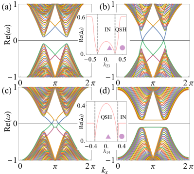
Figure 1: Topological phase transitions driven by non-Hermiticity. (a,b) The non-Hermitian term $i\lambda_{23}\Gamma_{23}$ drives the system from (a) trivial insulator ($\lambda_{23}=0.1$) to (b) QSH insulator ($\lambda_{23}=0.5$). The panels show open-boundary spectra on a zigzag ribbon. The parameters are $t=1$, $\lambda_{\text{SO}}=0.06$, $\lambda_{\nu}=0.4$ and $\lambda_{\text{Rb}}=0.05$. (c,d) The non-Hermitian term $i\lambda_{14}\Gamma_{14}$ drives the system from (c) QSH insulator ($\lambda_{14}=0.05$) to (d) trivial insulator ($\lambda_{14}=0.4$) with exceptional edge arcs. The parameters are the same as panels (a) and (b) except $\lambda_{\nu}=0.1$ and $\lambda_{\text{Rb}}=0$. The insets show the change of the real insulating gap Re($\Delta_{I}$) with respect to the non-Hermitian parameters. The dashed gray lines represent gap closing points, “IN” denotes the trivial insulator phase and the light purple triangles (disks) denote the non-Hermitian parameters for panels on the left (right).

We first consider the TR-symmetric non-Hermitian Kane-Mele model $H_{\text{nH-KM}}=H_{\text{KM}}\left(\bm{k}\right)+i\lambda_{23}\Gamma^{23}$. The term $i\lambda_{23}\Gamma^{23}$ mixes spins with non-Hermitian nearest-neighbor hopping, yielding asymmetry in the Rashba spin-orbit interaction along the bonds perpendicular to the zigzag edge. We start with a trivial insulator with strong sublattice potential $\lambda_{\nu}=0.4$. For a small $\lambda_{23}=0.1$, the open-boundary spectrum on a cylindrical geometry with zigzag edge is plotted in Fig. 1(a) and the edge states do not cross the band gap, showing a trivial insulator. For weak $\lambda_{23}$, the insulating gap scales as $\Delta_{I}=6\sqrt{3}\lambda_{\text{SO}}-\sqrt{-\lambda_{23}^{2}+\lambda_{\nu}^{2}}-\sqrt{-\lambda_{23}^{2}+\lambda_{\nu}^{2}+9\lambda_{\text{Rb}}^{2}}$ (the inset) with the gap closing at $\lambda_{23}^{c}=\pm\sqrt{(4\lambda_{\text{SO}}\lambda_{\nu})^{2}-3(\lambda_{\text{Rb}}-12\lambda_{\text{SO}})^{2}}/(4\lambda_{\text{SO}})\approx\pm 0.27$ for the given parameters. With increasing $\left|\lambda_{23}\right|>\left|\lambda_{23}^{c}\right|$, the gap reopens and the system enters the QSH phase with the emergence of helical edge states in the open-boundary spectrum at $\lambda_{23}=0.5$ (Fig. 1(b)). Surprisingly, the edge states in both regimes (trivial or topological) are purely real while the bulk spectrums are complex mySupp .

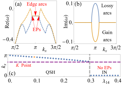
Figure 2: Exceptional points and exceptional edge arcs. (a,b) Real and imaginary parts of the edge states below the Fermi level. The parameters are the same as Figs. 1(c,d) except $\lambda_{14}=0.09$. The red arrows highlight the exceptional points (EPs) and edge arcs. (c) Evolution of (right) exceptional point along $k_{x}$ with respect to $\lambda_{14}$.

A different non-Hermitian term can also drive a phase transition from a QSH to a trivial insulator with exceptional properties of the helical edge states. We consider a QSH phase with $\lambda_{\nu}=0.1$ with vanishing Rashba spin-orbit interaction and add the non-Hermitian term $i\lambda_{14}\Gamma^{14}$. This term splits the degeneracies of the helical edge states at $k_{x}=\pi$ into two exceptional points (Fig. 1(c)), which are connected by two degenerate exceptional edge arcs with same real but opposite imaginary parts. This is illustrated in Figs. 2(a,b), where only the edge states below the Fermi level are plotted. The exceptional points are developed between two components in the helical edge state, which have opposite spins and chiralities (i.e., a TR-symmetric pair). Along the exceptional edge arc, the spins are no longer polarized.

The left and right exceptional points are symmetric to the $M$ point due to TR symmetry. In Fig. 2(c), we plot the position of the right exceptional point with respect to $\lambda_{14}$. It starts from the $M$ point ($k_{x}=\pi$) and moves almost linearly to $K$ point ($k_{x}=2\pi/3$), at which the insulating gap closes mySupp . The eigenenergies at $K$/$K^{\prime}$ points are $\pm\lambda_{\nu}\pm\sqrt{27\lambda_{\text{SO}}^{2}-\lambda_{14}^{2}}$, therefore the gap closes at $\lambda_{14}^{c}=\pm\sqrt{27\lambda_{\text{SO}}^{2}-\lambda_{\nu}^{2}}$. When the band gap reopens for $\lambda_{14}>\lambda_{14}^{c}$, the system becomes a trivial insulator, where the real insulating gap remains a constant Re$(\Delta_{I})=2\lambda_{\nu}$ (see inset of Figs. 1(c) and (d)). The exceptional edge arcs survive in the trivial insulator with constant real energies while exceptional points vanish. Such exceptional behaviors can be understood through a low-energy effective Hamiltonian of the helical edge states mySupp . We note that while similar edge arcs in Fig. 1(c) were observed previously KawabataK2019 , the non-Hermiticity-driven topological phase transition was not investigated.

Bulk biorthogonal $\mathbb{Z}_{2}$ invariant. The topological phase transition and the emergence of helical edge states indicate the change of the bulk topological invariant. In the Hermitian QSH phase with TR symmetry, the bulk topology is characterized by a $\mathbb{Z}_{2}$ index KaneZ22005 , which is obtained from the phase winding $\mathcal{W}=\frac{1}{2\pi i}\oint_{\mathcal{L}}d\bm{k}\cdot\nabla_{\bm{k}}\log\mathcal{P}(\bm{k})$ along a closed path $\mathcal{L}$ that encircles half of the Brillouin zone so that $\pm\bm{k}$ are not simultaneously included. Here $\mathcal{P}(\bm{k})$ is the Pfaffian $\mathcal{P}(\bm{k})=\text{Pf}(\langle u^{m}(\bm{k})|\mathcal{T}|u^{n}(\bm{k})\rangle)$, where $m,n$ enumerates the occupied bands and $|u^{n}(\bm{k})\rangle$ is the eigenvector. Because of the gauge-dependence of the Pfaffian, it is difficult to extend the Pfaffian $\mathbb{Z}_{2}$ to general non-Hermitian systems for describing non-Hermiticity-induced QSH insulators.

Here we establish a biorthogonal $\mathbb{Z}_{2}$ invariant for non-Hermitian TR-invariant QSH insulators by developing a non-Hermitian extension of the Wilson loop method RestaR1997 , which is equivalent to Kane-Mele Pfaffian definition in Hermitian systems YuR2011 . The biorthogonal Wilson line element is defined as

$$[G_{\alpha\beta}(\bm{k})]^{mn}={}_{\alpha}\langle u^{m}(\bm{k}+\Delta\bm{k})|u^{n}(\bm{k})\rangle_{\beta},\alpha\neq\beta,$$ (2)

where $\Delta\bm{k}=(\bm{k}_{f}-\bm{k}_{i})/N$ is a small fraction on a line constrained by two end points $\bm{k}_{i,f}$. $\alpha,\beta=L,R$ denote the left and right eigenvectors, which are defined as $H(\bm{k})|u(\bm{k})\rangle_{R}=\omega(\bm{k})|u(\bm{k})\rangle_{R}$ and $H^{\dagger}(\bm{k})|u(\bm{k})\rangle_{L}=\omega^{\ast}(\bm{k})|u(\bm{k})\rangle_{L}$. A normalization condition ${}_{\alpha}\langle u^{m}(\bm{k})|u^{n}(\bm{k})\rangle_{\beta}=\delta^{mn}$, $\alpha\neq\beta$ is imposed to form a biorthogonal system ShenH2018 .

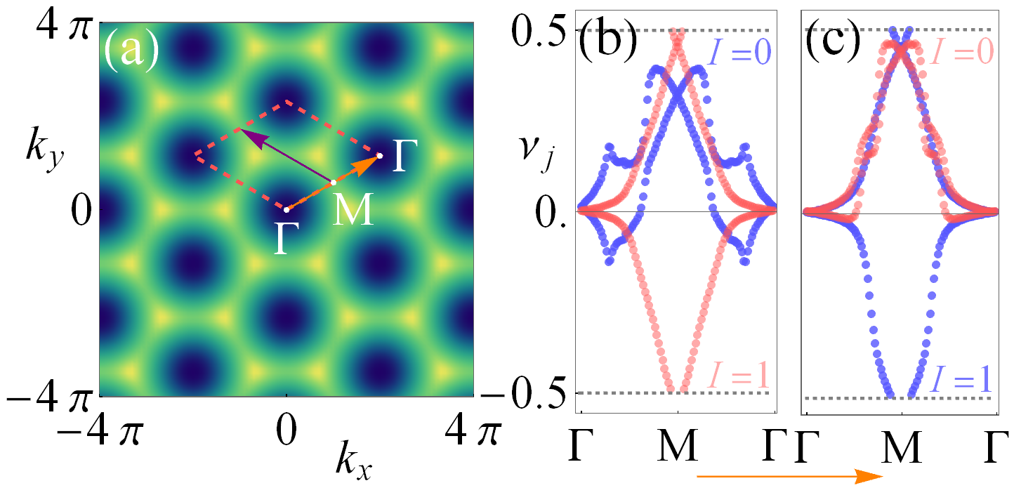
Figure 3: Bulk biorthogonal $\mathbb{Z}_{2}$ invariant from non-Hermitian Wilson loops. (a) The non-Hermitian Wilson loop in the Brillouin zone (dashed parallelogram) is defined along the purple arrow while the base point for each Wilson loop is given by the orange arrow. (b) and (c) The biorthogonal Wannier centers plotted to varying base points, corresponding to the cases in Figs. 1(a,b) and (c,d) respectively. The blue (red) points represent weak (strong) non-Hermitian effects and the biorthogonal $\mathbb{Z}_{2}$ index $I$ is labeled in each panel.

A path-ordered discrete Wilson line is defined as $\mathcal{W}_{\bm{k}_{i}\rightarrow\bm{k}_{f}}=G(\bm{k}_{f}-\Delta\bm{k})G(\bm{k}_{f}-2\Delta\bm{k})...G(\bm{k}_{i}+\Delta\bm{k})G(\bm{k}_{i})$ with

$$[G(\bm{k})]^{mn}=\frac{1}{2}\left([G_{LR}(\bm{k})]^{mn}+[G_{RL}(\bm{k})]^{mn}\right).$$ (3)

A Wilson loop $\mathcal{W}_{\bm{k}_{i}\rightarrow\bm{k}_{i}+\bm{T}}$, i.e., a closed Wilson line, starts from the base point $\bm{k}_{i}$, and returns to $\bm{k}_{f}=\bm{k}_{i}+\bm{T}=\bm{k}_{i}$ after a period $\bm{T}$. The biorthogonal Wannier center $\nu_{j}(\bm{k}_{i})$ for each $\bm{k}_{i}$ is defined as the phase of the eigenvalues $E_{j}^{N}(\bm{k}_{i})=e^{i2\pi\nu_{j}(\bm{k}_{i})}$ of the Wilson loop through $\mathcal{W}_{\bm{k}_{i}\rightarrow\bm{k}_{i}+\bm{T}}(\bm{k})|v_{j}(\bm{k}_{i})\rangle_{R}=E_{j}^{N}(\bm{k}_{i})|v_{j}(\bm{k}_{i})\rangle_{R}$ (in this work, $j=1,2$ for two lower occupied bands) and can be physically interpreted as the relative position of the particle to the center of one unit cell mySupp .

The biorthogonal $\mathbb{Z}_{2}$ invariant $I=\eta_{j}\mod 2$ is defined by the winding $\eta_{j}=\frac{1}{2\pi}\oint_{\mathcal{C}}\nabla_{\bm{k}}\nu_{j}(\bm{k}_{i})\cdot d\mathbf{k}_{i}$ for each pair of biorthogonal Wannier centers, where $\mathcal{C}$ is a loop for the base point $\bm{k}_{i}$ in the Brillouin zone. $I=1$ corresponds to the topological QSH insulator with helical edge states for odd $\eta_{j}$, while $I=0$ corresponds to trivial insulator without any topologically protected edge state for even $\eta_{j}$. When TR symmetry is preserved, the winding of each biorthogonal Wannier center must come with its TR-symmetric pair (either two 0 or a pair like $\pm 1$), therefore the biorthogonal $\mathbb{Z}_{2}$ invariant can always be defined.

To compute the biorthogonal Wannier center $\nu_{j}(\bm{k}_{i})$ on the honeycomb lattice, we choose the Brillouin zone shown in Fig. 3(a). The base point $\bm{k}_{i}$ is chosen along the orange arrow while the purple arrow defines each non-Hermitian Wilson loop. The computed $\nu_{j}(\bm{k}_{i})$ for the QSH phase is displayed in Fig. 3(b), where the blue and red dots correspond to Figs. 1(a,b) respectively. There are two $\nu_{j}(\bm{k}_{i})$ for each color since there are two occupied bands. The path $\mathcal{C}$ for the base point $\bm{k}_{i}$ starts from the $\Gamma$ point, sweeps through the $M$ point and finally ends at another $\Gamma$ point, with $\nu_{j}(\bm{k}_{i})$ symmetric to $M$ point. At TR-symmetric points ($\Gamma$ and $M$), $\nu_{j}(\bm{k}_{i})$ are degenerate as Kramers’ pairs. Inversion symmetry dictates that $\nu_{j}(\bm{k}_{i})$ must have opposite signs so that they vanish at $\Gamma$. In the topological regime, $\nu_{j}(\bm{k}_{i})$ travel along different directions and show windings $\eta_{j}=\pm 1$, yielding a biorthogonal $\mathbb{Z}_{2}$ index $I=1$ (red dots). In the trivial insulator regime, $\nu_{j}(\bm{k}_{i})$ never crosses $\pm 1/2$ and the winding vanishes, yielding $I=0$ (blue dots). Similarly, the topological phase transition driven by $i\lambda_{14}\Gamma^{14}$ in Figs. 1(c,d) is consistent with the change of bulk biorthogonal $\mathbb{Z}_{2}$ invariant from blue ($I=1$) to red ($I=0$) dots in Fig. 3(c).

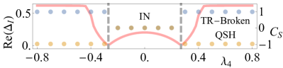
Figure 4: Biorthogonal spin Chern number as the topological invariant for TR-broken non-Hermitian QSH insulator. The parameters are the same as in Figs. 1(a,b). The blue ($S=1/2$, spin “up”) and orange ($S=-1/2$, spin “down”) dots are biorthogonal spin Chern numbers $C_{S}$. The red curve represents the real insulating gap.

Biorthogonal spin Chern number for TR-broken non-Hermitian QSH insulators. When TR symmetry is broken, the windings of Wannier centers may not come in pairs, therefore the biorthogonal $\mathbb{Z}_{2}$ invariant cannot be defined. Moreover, without TR symmetry, the system reduces to the symmetry class classified by a $\mathbb{Z}$ topological invariant KawabataK2018 . Here we consider a generalization of the spin Chern number, which, in Hermitian systems, consists of a non-trivial decomposition of a trivial Bloch bundle ProdanRobustness2009 .

We construct a biorthogonal $M$ matrix

$$[M(\bm{k})]^{mn}={}_{L}\langle u^{m}(\bm{k})|\tau_{0}\otimes s_{z}|u^{n}(\bm{k})\rangle_{R},$$ (4)

whose diagonalization decomposes the mixed occupied bands into two spin sectors (denoted by $S=\pm 1/2$) satisfying $M(\bm{k})|\psi_{S}(\bm{k})\rangle_{R}=\omega_{S}|\psi_{S}(\bm{k})\rangle_{R}$. When the eigenspectra $\omega_{S}$ of two spin sector are separable, we can define the biorthogonal spin Chern number for each spin sector $C_{S,\alpha\beta}=\frac{1}{2\pi}\int d^{2}\bm{k}\cdot\mathcal{F}_{S,\alpha\beta}(\bm{k})$ through the Berry curvature $\mathcal{F}_{S,\alpha\beta}(\bm{k})=\nabla\times\mathcal{A}_{S,\alpha\beta}(\bm{k})$, where the non-Abelian Berry connection

$$\mathcal{A}_{S,\alpha\beta}(\bm{k})=-i{}_{\alpha}\langle\psi_{S}(\bm{k})\cdot\bm{u}(\bm{k})|\partial_{\bm{k}}|\psi_{S}(\bm{k})\cdot\bm{u}(\bm{k})\rangle_{\beta},$$ (5)

and $|\psi_{S}(\bm{k})\cdot\bm{u}(\bm{k})\rangle_{\beta}=\sum_{j}\psi_{j}(\bm{k})|u^{j}(\bm{k})\rangle_{\beta}$. The summation of $j$ runs over all occupied bands and $\psi_{j}(\bm{k})$ denotes the $j$-th component of the eigenvector $|\psi_{S}(\bm{k})\rangle_{\beta}$. Previous studies have shown that the Chern numbers defined through different Berry curvatures from left or right eigenvectors are equivalent due to their gauge-invariant nature ShenH2018 . Similar arguments apply here, and we denote $C_{S}=C_{S,\alpha\beta}$ hereafter.

In our context, a non-zero biorthogonal spin Chern number $C_{S}$ means there is a chiral edge state of “spin-$S$” with the chirality determined by the sign of $C_{S}$. This is not generally true ProdanRobustness2009 but holds here because the underlying Haldane model is a Chern insulator with the topological invariant quantized to 0 and $\pm 1$ HaldaneModel1998 . In the trivial insulator phase $C_{\pm 1/2}=0$, while $C_{\pm 1/2}=\pm 1$ in QSH phase. In the integer quantum Hall phase, $C_{\pm 1/2}=1$ or $-1$ mySupp . Because $C_{S}$ is developed without symmetry constraint, it can be applied in the TR-symmetric region. In fact, the biorthogonal spin Chern number provides an equivalent description as the biorthogonal $\mathbb{Z}_{2}$ invariant in the TR-symmetric region mySupp .

The QSH phase survives even when TR-symmetry is broken except that there are small backscatterings on the helical edge states, which open a small energy gap on the edge states near the Fermi level YangTime2011 . Such a TR-broken QSH phase can also be achieved directly from a trivial phase through non-Hermiticity. For instance, we consider a term $i\lambda_{4}\Gamma^{4}$ that breaks TR symmetry, and start from a trivial insulator phase as in Fig. 1(a). This term also renders asymmetric Rashba spin-orbit interaction and the gap scales similarly as the inset in Figs. 1(a,b). With increasing $|\lambda_{4}|$, the gap closes and then reopens, leading to a TR-broken QSH phase, as shown in Fig. 4. The biorthogonal spin Chern numbers $C_{S}$ for both trivial insulator and TR-broken QSH phases are computed, which are consistent with the open-boundary spectra (see Fig. S4 in Supplemental Materials mySupp ). In Hermitian systems, a topological phase transition from a TR-broken QSH phase to an interger quantum Hall phase can be driven by a real exchange field $\lambda_{\mu}\Gamma^{34}$. Such a phase transition still exists in the non-Hermitian region and can be characterized by the biorthogonal spin Chern number mySupp .

Conclusion and Discussion. In summary, we have demonstrated that QSH insulators and their phase transitions from/to trivial insulators can be driven by non-Hermiticity and showcased the exceptional edge arcs under topological phase transition. While our discussion focuses on non-Hermitian Kane-Mele model, the developed topological invariants, i.e., the biorthogonal $\mathbb{Z}_{2}$ index and spin Chern number $C_{S}$, are applicable to other QSH models like non-Hermitian BHZ model. The biorthogonal $\mathbb{Z}_{2}$ index may be further generalized to characterize 3D non-Hermitian topological insulators, which needs further investigation. The biorthogonal $\mathbb{Z}_{2}$ (and $\mathbb{Z}$) topological invariants provide a powerful tool for characterizing wide classes of non-Hermitian topological matters and pave the way for exploring their device applications.

Appendix A Supplemental Materials for “Non-Hermitian topological phase transitions for quantum spin Hall insulators”

The Supplemental Materials provide more details on imaginary bands, exceptional points on helical edge states, non-Hermitian Wilson line in thermodynamic limits, biorthogonal spin Chern number as topological invariant for TR-symmetric non-Hermitian QSH insulators, edge states of non-Hermiticity-driven TR-broken QSH phase and non-Hermitian IQH phase.

A.1 Imaginary bands of open-boundary spectra

For the convenience of the reader, we list the non-zero coefficients of the Kane-Mele model KaneZ22005

$$d_{1} = t\left(1+2\cos\left(\frac{1}{2}k_{x}\right)\cos\left(\frac{\sqrt{3}}{2}k_{x}\right)\right),$$

$$d_{2} = \lambda_{\nu},$$

$$d_{3} = \lambda_{\text{Rb}}\left(1-\cos\left(\frac{1}{2}k_{x}\right)\cos\left(\frac{\sqrt{3}}{2}k_{x}\right)\right),$$

$$d_{4} = -\sqrt{3}\lambda_{\text{Rb}}\ \sin\left(\frac{1}{2}k_{x}\right)\sin\left(\frac{\sqrt{3}}{2}k_{x}\right),$$

$$d_{12} = -2t\cos\left(\frac{1}{2}k_{x}\right)\sin\left(\frac{\sqrt{3}}{2}k_{x}\right),$$

$$d_{15} = 2\lambda_{\text{SO}}\ \left(\sin k_{x}-2\cos\left(\frac{1}{2}k_{x}\right)\cos\left(\frac{\sqrt{3}}{2}k_{x}\right)\right),$$

$$d_{23} = -\lambda_{\text{Rb}}\ \cos\left(\frac{1}{2}k_{x}\right)\sin\left(\frac{\sqrt{3}}{2}k_{x}\right),$$

$$d_{24} = \sqrt{3}\lambda_{\text{Rb}}\ \sin\left(\frac{1}{2}k_{x}\right)\cos\left(\frac{\sqrt{3}}{2}k_{x}\right),$$

$$d_{34} = \lambda_{\mu},$$

where the last term represents a TR-broken exchange field and is introduced in TR-broken QSH insulators YangTime2011 .

In the main text, we examine two topological phase transitions in the TR-symmetric non-Hermitian Kane-Mele model. Only real parts of the open-boundary spectra are plotted in the main text (see Fig. 1). The imaginary bands are plotted here in Fig. S1.

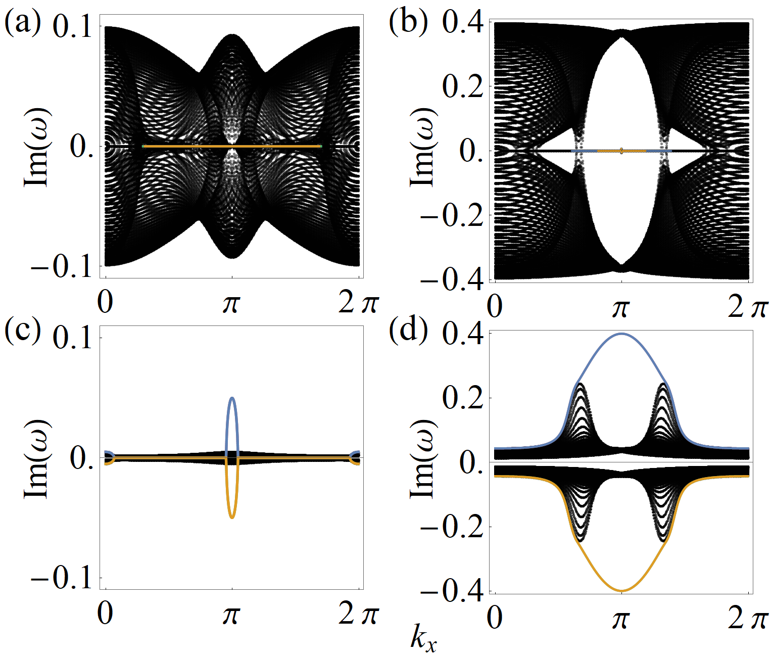
Figure S1: Imaginary bands in TR-symmetric non-Hermitian Kane-Mele model. (a-d) Imaginary parts of the spectra shown in Figs. 1(a-d) respectively. The edge states are plotted with the same color as those in Fig. 1 and we only plot the purely real edge states in panels (a) and (b).

For the topological phase transition from trivial to QSH insulators driven by non-Hermitian term $i\lambda_{23}\Gamma^{23}$, the edge states in both phases are (mostly) purely real while the bulk spectrum is complex, as shown in Figs. S1(a,b). The helical edge states are separated from the bulk bands in the entire complex plane.

Different from asymmetric Rashba spin-orbit interaction $i\lambda_{23}\Gamma^{23}$, $i\lambda_{14}\Gamma^{14}$ term represents a non-Hermitian next-nearest-neighbor hopping that only mixes spins. It splits the edge crossing into a pair of exceptional points, which are connected by an exceptional edge arc with same real energy and opposite imaginary energies, as shown in Fig. S1(c). Outside the exceptional edge arc, the edge state spectrum is purely real. In the trivial insulator phase, the entire spectrum becomes complex (see Fig. S1(d)).

A.2 Bulk bands and low-energy theory of exceptional edge arcs

A non-zero $\Gamma_{14}$ term couples different spins while preserves the sublattice degree of freedom. With a real coefficient, $\lambda_{14}\Gamma_{14}$ breaks the TR symmetry and opens a finite gap on the helical edges. There is no gap closing or topological phase transition. In contrast, the imaginary term $i\lambda_{14}\Gamma_{14}$ generates a pair of exceptional points on the gapless helical edge states that cross at TR-symmetric points. Two similar terms are $i\lambda_{13}\Gamma_{13}$ and $i\lambda_{35}\Gamma_{35}$, which can also induce topological phase transitions through splitting the edge crossings into exceptional points.

In the main text, we have described the properties of exceptional edge arcs. Here we plot the change of the bulk band spectrum across the phase transition with the band gap closing in Figs. S2(a) and (b). The gap closing happens in the complex plane, meaning both real and imaginary parts of the eigenvalues must vanish.

A similar picture holds when Rashba spin-orbit interaction exists or TR symmetry is broken by a small exchange field $\lambda_{34}\Gamma^{34}$. The Rashba term turns the real edge states outside the exceptional edge arcs into complex states and the exchange field simply shifts the exceptional points to different directions. The topological phase transition driven by $i\lambda_{14}\Gamma^{14}$ with small Rashba spin-orbit interaction (the system is still topological when $\lambda_{14}=0$) is plotted in Fig. S2(c). The critical points for the phase transition become gapless phases and the biorthogonal $\mathbb{Z}_{2}$ index developed in the main text still applies. Finally, we note that one can change the open-boundary direction and observe the same physics along $k_{y}$.

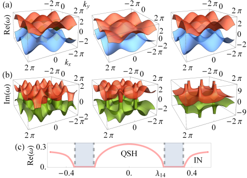
Figure S2: (a,b) Real and imaginary bands in momentum space across the phase transition. The parameters are $\lambda_{14}=0.2$, $0.295$ (gap closing point) and $0.4$. (c) Topological phase transition driven by $i\lambda_{14}\Gamma_{14}$ with nonzero Rashba spin-orbit interaction. The parameters are the same as those in Fig. 2 in the main text except $\lambda_{\text{Rb}}=0.05$. The light-blue-coded areas correspond to the gapless phases.

To understand how a non-Hermitian term induces exceptional points on the helical edge states, we consider a low-energy effective Hamiltonian

$$H_{\text{edge}}=k_{x}\Gamma_{15}+\lambda_{\nu}\Gamma_{2}+i\lambda_{14}\Gamma_{14},$$ (6)

which preserves the TR symmetry. The first term $k_{x}\Gamma_{15}$ describes a Dirac fermion with the four-fold degeneracy at $k_{x}=0$. The second term $\lambda_{\nu}\Gamma_{2}$ lifts the degeneracy and renders 4 edge crossings, two of which locate at the Fermi level with opposite $k_{x}$ while the other two at $k_{x}=0$ with opposite energies. Such a band structure resembles the edge spectrum in a QSH insulator. The last term $i\lambda_{14}\Gamma_{14}$ stretches each band crossing below and above the Fermi level into two exceptional points. Diagonalize the above Hamiltonian, we obtain

$$\omega_{\pm,-}=\pm\sqrt{k_{x}^{2}-\lambda_{14}^{2}}-\lambda_{\nu},\omega_{\pm,+}=\pm\sqrt{k_{x}^{2}-\lambda_{14}^{2}}+\lambda_{\nu},$$ (7)

$$|\psi_{\pm,-}\rangle_{R}=(0,-\frac{k_{x}-\omega_{\pm,-}-\lambda_{\nu}}{\lambda_{14}},0,1)^{T},~{}|\psi_{\pm,+}\rangle_{R}=(-\frac{k_{x}+\omega_{\pm,+}-\lambda_{\nu}}{\lambda_{14}},0,1,0)^{T},$$ (8)

where $\omega_{\pm,\pm}$ denote four eigenvalues and $|\psi_{\pm,\pm}\rangle_{R}$ are the corresponding right eigenvectors. Both the eigenvalues and the right eigenvectors collapse at the exceptional points $k_{x}=\pm\lambda_{14}$ (so do the left eigenvectors). In general, exceptional points are not protected by TR symmetry. If the TR symmetry is broken with an exchange field $\lambda_{34}\Gamma_{34}$, the exceptional points merely shift their positions to $k_{x}=\pm\lambda_{14}-\lambda_{34}$ (for the pair above the Fermi level) or $k_{x}=\pm\lambda_{14}+\lambda_{34}$ (for the pair below the Fermi level). We also note that the topological phase transition studied in Figs. 1(c,d) still occurs in TR-broken non-Hermitian QSH insulators.

A.3 Biorthogonal Wilson line in thermodynamic limit

In non-Hermitian systems, the Berry connection cannot be solely defined through the right eigenvectors. A proper way to define a purely real Berry connection involves both left and right eigenvectors

$$\mathcal{A}(\bm{k})=\frac{1}{2}\left(\mathcal{A}_{LR}(\bm{k})+\mathcal{A}_{RL}(\bm{k})\right),$$ (9)

where $[\mathcal{A}_{\alpha\beta}(\bm{k})]^{mn}=-i{}_{\alpha}\langle u^{m}(\bm{k})|\partial_{\bm{k}}u^{n}(\bm{k})\rangle_{\beta}$, $\alpha\neq\beta$ is the biorthogonal non-Abelian Berry connection. $\mathcal{A}(\bm{k})$ is real since $\mathcal{A}_{LR}(\bm{k})=\mathcal{A}_{RL}^{\ast}(\bm{k})$.

To justify our definition of the non-Hermitian Wilson line element

$$[G(\bm{k})]^{mn}=\frac{1}{2}\left([G_{LR}(\bm{k})]^{mn}+[G_{RL}(\bm{k})]^{mn}\right)$$ (10)

in the main text, we need show that the non-Hermitian Wilson line gives the desired non-Hermitian Berry phase in the thermodynamic limits, similar to the Hermitian cases RestaR1997 . We expand each element $[G_{\alpha\beta}(\bm{k})]^{mn}={}_{\alpha}\langle u^{m}(\bm{k}+\Delta\bm{k})|u^{n}(\bm{k})\rangle_{\beta}$ to the first order (assuming $N$ is very large)

$$[G_{\alpha\beta}(\bm{k})]^{mn}={}_{\alpha}\langle u^{m}(\bm{k})|u^{n}(\bm{k})\rangle_{\beta}+(\Delta\bm{k}){}_{\alpha}\langle\partial_{\bm{k}}u^{m}(\bm{k})|u^{n}(\bm{k})\rangle_{\beta}.$$ (11)

Due to the normalization condition ${}_{\alpha}\langle u^{m}(\bm{k})|u^{n}(\bm{k})\rangle_{\beta}=\delta^{mn}$ ShenH2018 , we have ${}_{\alpha}\langle\partial_{\bm{k}}u^{m}(\bm{k})|u^{n}(\bm{k})\rangle_{\beta}=-{}_{\alpha}\langle u^{m}(\bm{k})|\partial_{\bm{k}}u^{n}(\bm{k})\rangle_{\beta}$. The biorthogonal Wilson line element can be rewritten as

$$[G_{\alpha\beta}(\bm{k})]^{mn}=\delta^{mn}-i(\Delta\bm{k})[\mathcal{A}_{\alpha\beta}(\bm{k})]^{mn},$$ (12)

yielding

$$[G(\bm{k})]^{mn}=\delta^{mn}-i(\Delta\bm{k})[\mathcal{A}(\bm{k})]^{mn}.$$ (13)

The non-Hermitian Wilson loop from $\bm{k}_{i}$ to $\bm{k}_{f}$ is defined through a path-ordered multiplication

$$\mathcal{W}_{\bm{k}_{i}\rightarrow\bm{k}_{f}}=\prod_{j=1}^{N}\left(I_{0}-i(\Delta\bm{k})\mathcal{A}(\bm{k}+j\Delta\bm{k})\right),$$ (14)

where $I_{0}$ is the identity matrix. Under the thermodynamic limit $N\rightarrow\infty$, it gives the exponential of the non-Hermitian Berry phase

$$\lim_{N\rightarrow\infty}\mathcal{W}_{\bm{k}_{i}\rightarrow\bm{k}_{f}}=e^{-i\int_{\bm{k}_{i}}^{\bm{k}_{f}}\mathcal{A}(\bm{k})\cdot d\bm{k}}.$$ (15)

This equation demands that the non-Hermitian Wilson loop must be unitary in the thermodynamic limit so that the biorthogonal Wannier center can be defined.

Since the Berry phase represents the electronic contribution to the dielectric polarization in solid state, the biorthogonal Wannier center $\nu_{j}(\bm{k})$ can be physically interpreted as the relative position of the particle to the center of one unit cell with the polarization

$$p=-\frac{i}{2\pi}\log\det(\mathcal{W}_{\bm{k}_{i}\rightarrow\bm{k}_{i}+\bm{T}}).$$ (16)

A.4 Biorthogonal spin Chern number in TR-symmetric non-Hermitian QSH insulators

In the main text, we claim that biorthogonal spin Chern number also works when TR-symmetry is preserved. Here we use the biorthogonal spin Chern number to characterize two topological phase transitions studied in Fig. 1.

The first topological phase transition from a trivial insulator to a QSH insulator is driven by the non-Hermitian term $i\lambda_{23}\Gamma_{23}$. We compute the biorthogonal spin Chern number for a wild range of $\lambda_{23}$, as shown in Fig. S3(a). In the trivial insulator phase, we have both $C_{\pm 1/2}=0$ as expected. Across the phase transition point, the biorthogonal spin Chern number abruptly changes to $C_{\pm 1/2}=\pm 1$, corresponding to the non-Hermitian QSH phase.

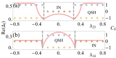
Figure S3: Biorthogonal spin Chern number as topological invariant for TR-symmetric non-Hermitian QSH insulators. (a,b) Biorthogonal spin Chern numbers computed for the TR-symmetric models in Figs. 1(a,b) and (c,d), respectively.

The other topological phase transition is ascribed to the non-Hermitian term $i\lambda_{14}\Gamma_{14}$. Since we start from the QSH phase, we have $C_{\pm 1/2}=\pm 1$ when $|\lambda_{14}|$ is relatively small, as shown in Fig. S3(b). In the trivial insulator phase, the biorthogonal spin Chern numbers vanish $C_{\pm 1/2}=0$.

From these examples, we see that the biorthogonal spin Chern number correctly characterizes the topological properties of the TR-symmetric non-Hermitian Kane-Mele model. It provides an equivalent description as the biorthogonal $\mathbb{Z}_{2}$ invariant. While a rigor proof of such equivalence is hard to formulate, similar conclusion has been drawn in Hermitian systems through the argument that the spin Chern numbers do not contain more information than the $\mathbb{Z}_{2}$ invariant and vice versa ProdanRobustness2009 . Similar arguments may be generalized to the non-Hermitian cases.

A.5 TR-broken QSH phase driven by non-Hermiticity

In the main text, we use the biorthogonal spin Chern number to characterize a topological phase transition from a trivial insulator phase to a TR-broken QSH phase driven by the non-Hermitian term $i\lambda_{4}\Gamma^{4}$, as shown in Fig. 4.

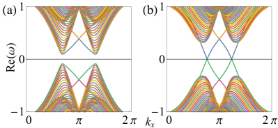
Figure S4: TR-broken QSH phase driven by the non-Hermitian term $i\lambda_{4}\Gamma^{4}$. Open-boundary spectrum is plotted for (a) trivial insulator phase ($\lambda_{4}=0.1$) and (b) TR-broken QSH phase ($\lambda_{4}=0.5$). Other parameters are the same as those in Figs. 1(a) and (b).

In Fig. S4(a), we plot the open-boundary spectrum for $\lambda_{4}=0.1$, corresponding to a trivial insulator phase. The edge states do not cross the band gap. With the increasing non-Hermitian strength, the system enters the topological region. An example of $\lambda_{4}=0.5$ is displayed in Fig. S4(b), where a typical edge configuration for the QSH phase in the Kane-Mele model is found. The edge states are consistent with the prediction from the biorthogonal spin Chern number, demonstrating the bulk-edge correspondence.

A.6 IQH phases in TR-broken non-Hermitian QSH insulators

Previous study in Hermitian systems has incorporated the spin Chern number to characterize the phase transition from a TR-broken QSH phase to an IQH phase YangTime2011 . Here, we show that such a topological phase transition still exists in non-Hermitian systems and their topological properties are characterized by the biorthogonal spin Chern number.

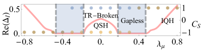
Figure S5: Biorthogonal spin Chern number as the topological invariant for TR-broken non-Hermitian QSH insulators. The topological phase transition is induced by a real exchange field $\lambda_{\mu}\Gamma_{34}$ and a small non-Hermitian term $i0.05\Gamma_{14}$ is included. Other parameters are the same as those in Figs. 1(a,b).

We consider a non-Hermitian Kane-Mele model with a small non-Hermitian term $i\lambda_{14}\Gamma_{14}$ and a real exchange field $\lambda_{\mu}\Gamma_{\mu}$. The biorthogonal spin Chern number with varying exchange field is plotted in Fig. S5. In the TR-broken QSH phase, the biorthogonal spin Chern number remains non-trivial $C_{\pm 1/2}=\pm 1$. With increasing exchange field, we observe a gapless phase and finally a non-Hermitian IQH phase, where both spin sectors have the same biorthogonal spin Chern number depending on the sign of the exchange field $C_{\pm 1/2}=\text{sign}(\lambda_{\mu})$. The spin Hall current vanishes but the charge Hall conductance is quantized to $2$ (not strictly due to the Rashba spin-orbit interaction and non-Hermitian effects).