Optimal Transport Flows for Distributed Production Networks

Abstract

Network flows often exhibit a hierarchical tree-like structure that can be attributed to the minimisation of dissipation. The common feature of such systems is a single source and multiple sinks (or vice versa). In contrast, here we study networks with only a single source and sink. These systems can arise from secondary purposes of the networks, such as blood sugar regulation through insulin production. Minimisation of dissipation in these systems lead to trivial behaviour. We show instead how optimising the transport time yields network topologies that match those observed in the insulin-producing pancreatic islets. These are patterns of periphery-to-center and center-to-periphery flows. The obtained flow networks are broadly independent of how the flow velocity depends on the flow flux, but continuous and discontinuous phase transitions appear at extreme flux dependencies. Lastly, we show how constraints on flows can lead to buckling of the branches of the network, a feature that is also observed in pancreatic islets.

Transport networks are essential for life to function on large multicellular scales. In vertebrates, blood flow delivers energy and nutrients, and removes waste through the branched network of the vascular system. The separation of vessels into arteries and veins ensures that oxygen-rich and oxygen-depleted parts of the network are kept separate. In plants the separation into xylem and phloem provides a similar function. In nature, these systems typically exhibit tree-like hierarchical structures, as e.g. in the aorta which splits into increasingly smaller arteries all the way to capillaries, the smallest vessels of the circulatory system. The tree structure can be understood as minimising the dissipation of the blood flow through the system Bohn2007 ; Hu2013 ; Ronellenfitsch2016 . Furthermore, loop-redundant tree-like structures, as is evident from observing e.g. the veins of a tree leaf, is explained by minimising dissipation under damage or under fluctuating needs Katifori2010 ; Corson2010 . Perhaps because of its origin as a power-minimising network, tree-like structures are observed not just in vascular networks, but also for instance in both natural and artificial river networks Dodds2010 ; Katifori2010 . The shared feature of these systems is that they consists of a single fluid source with a lot of sinks, or a single sink with a lot of sources (these are equivalent, dual formulations). For instance, in the arterial system the heart is the source and the body cells the sinks, whereas the roles are reversed in venous systems.

The study of flow networks that have a single source and a single sink have received much less attention, perhaps because it is not clear what properties can be optimised over such networks — indeed dissipation minimisation lead to trivial behaviour. However, such networks are critical in flow systems that have secondary products (e.g. other than oxygen in blood) that are being produced or delivered along the flow path. Here, we exemplify such a system by the Islets of Langerhans in the pancreas. In these islets, beta cells release insulin and alpha cells glucagon into the blood stream based on blood glucose levels Pour2002 ; Hong2013 . In such systems there is no need for an arterial-venous separation, and the transport from any hormone-producing cell directly couples to both the downstream and upstream transport systems.

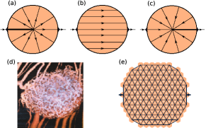
Figure 1: Vasculature of pancreatic islets. (a) Center-to-periphery flow. (b) Left-right symmetric flow. (c) Periphery-to-center flow. (d) Microscopy of vasculature, from Ref. Berclaz2016 , showing the high degree of tortuousness in the vasculature of pancreatic islets. (e) The network structure considered. This is constructed by taking a circular subsection of a hexagonal grid of nodes. Neighbours are then induced from a Delaunay triangulation. Each edge has a conductivity $C_{e}$ associated to it, which are the parameters to be optimised over. Inlet and outlet are shows by arrows.

The vasculature of pancreatic islets differs from species to species. In particular, various topologies have been observed: periphery-to-center flow, straight through, and center-to-periphery flow, as illustrated in Fig. 1(a-c) Shimokawa1988 ; Nyman2008 ; El-gohary2018 . For instance in rodents, the center-to-periphery topology is the most common Nyman2008 . furthermore, the vasculature of these islets is often very tortuous compared to the vasculature of other organs Berclaz2016 ; Kirkegaard2019 as shown in Fig. 1d. In this Letter we propose an optimisation problem over single-source, single-sink flows and use this to provide possible explanations for the type of features observed in pancreatic islets.

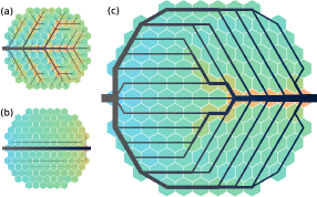
Figure 2: Optimised network structures. (a) Minimal dissipation network with sinks at all nodes. (b) Minimal dissipation network with a single sink at edge. (c) Per-node time minising network with a single sink at edge. Cell colours indicate product concentration flowing through that node as calculated by solving $\rho_{i}=1+\sum_{j\in\mathcal{I}_{i}}|F_{ij}|\,\rho_{j}/\sum_{k\in\mathcal{O}_{j}}|F_{jk}|$ ($\mathcal{I}_{i}$ denoting incoming and $\mathcal{O}_{i}$ outgoing nodes of node $i$). Flow lines are coloured by pressure, their thickness indicating (square root of) flow magnitude.

Model — To study systems of blood flow optimisation we consider, as in previous studies Bohn2007 ; Hu2013 ; Katifori2010 ; Ronellenfitsch2016 ; Corson2010 , flows on networks. While pancreatic islets indeed can have more than one inlet and outlet, we simplify the system and consider the network shown in Fig. 1e. Nevertheless, our approach works for any number of sources and sinks. In Fig. 1e cells are represented by hexagons, and edges betweens between these cells indicate where fluid can potentially flow. Inlet and outlet are indicated by arrows.

This specific graph has $n_{N}=130$ nodes and $n_{E}=357$ edges, and each edge $e$ of the graph has a conductivity $C_{e}$ and a length $L_{e}$. An $n_{E}\times n_{N}$ oriented incident matrix $\Delta$ of the graph gives each edge a unique direction, and we can thus attach to each edge a (signed) flow $F_{e}$. We furthermore define the source vector ${\boldsymbol{S}}$ with $S_{\text{source}}=1$, $S_{\text{sink}}=-1$ and $S_{i}=0$ elsewhere and require that the flow obeys Kirchoff’s current law

$$\Delta^{T}{\boldsymbol{F}}={\boldsymbol{S}}.$$ (1)

Since $n_{N}<n_{E}$, the flow is far from determined by this condition alone.

To make the flow well-defined, we furthermore require that it is derivable from a potential based on the effective conductivities,

$${\boldsymbol{F}}={\boldsymbol{C}}^{\text{eff}}\Delta{\boldsymbol{p}},$$ (2)

where $p_{i}$ is the potential (pressure) defined at the nodes, and ${\boldsymbol{C}}^{\text{eff}}$ is a diagonal matrix with entries $C^{\text{eff}}_{ee}=C_{e}/L_{e}$. Combining Eq. (1) and (2) we can solve for the potential as

$${\boldsymbol{p}}=[\Delta^{T}{\boldsymbol{C}}^{\text{eff}}\Delta]^{\dagger}\,{\boldsymbol{S}},$$ (3)

where $\dagger$ denotes the pseudo-inverse, which is needed since the system of equations is singular, but can be solved by the pseudo-inverse if $\sum_{i}S_{i}=0$, which is indeed the case here. From the potentials ${\boldsymbol{p}}$, the flows are immediately obtained from Eq. (2).

The total power dissipation of the system is $P=\sum_{e}F_{e}^{2}/C^{\text{eff}}_{ee}$ Bohn2007 ; Hu2013 ; Ronellenfitsch2016 . As mentioned, minimising this term leads to tree topologies for a single source and sinks everywhere ($S_{\text{source}}=1$, $S_{i}=-1/(n_{N}-1)$ elsewhere). This optimum on our network topology is shown in Fig. 2a. The minimisation is done under constant “material cost” $\sum_{e}L_{e}C_{e}^{\gamma}$, and the tree-like structures are obtained for $\gamma<1$. In the optimum, the conductivities scale with the flow as Briefly, minimising $\sum_{e}L_{e}F_{e}^{2}/C_{e}$ under constant $\sum_{e}L_{e}C_{e}^{\gamma}$ by the method of Lagrange multipliers leads to $-F_{e}^{2}/C_{e}^{2}+\lambda\gamma C_{e}^{\gamma-1}=0$ from which the scaling follows. See e.g. Ref. Bohn2007 for details.

$$C_{e}\sim|F_{e}|^{2/(1+\gamma)},$$ (4)

i.e. a larger conductivity is needed where there is a lot of flow.

Trivially, minimising power dissipation in the network with just a single source and single sink leads to flow only going along the shortest path between the source and sink as shown in Fig. 2b. This is also, naturally, the time minimising network for flow between the source and the sink. We are interested in network structures that visit all nodes in an “optimal” way. Indeed proper distribution of vessels is far more important in pancreatic islets and other systems than the (potentially miniscule) power being dissipated.

We consider instead graphs that minimise the average time for the product (e.g. insulin) being produced at the nodes to reach the outlet (the opposite inlet-centric definition will be discussed later). This time-optimised graph we define as follows: Denote for each node $T_{i}$ the average time taken from that node for product to reach the outlet. The average time that we intend to minimise is thus

$$\langle T\rangle=\frac{1}{n_{N}}\sum T_{i},$$ (5)

where $T_{i}$ is found by the recursive relation which follows by letting product flow in proportion to the fluid flow,

$$T_{i}=\frac{\sum_{j\in\mathcal{O}_{i}}|F_{ij}|\,(T_{j}+T_{ij})}{\sum_{j\in\mathcal{O}_{i}}|F_{ij}|},$$ (6)

with the special case $T_{\text{sink}}=0$. This is a linear equation for $T_{i}$, where $\mathcal{O}_{i}$ is the set of nodes that are outgoing from node $i$. Whether an edge $e$ is outgoing from node $i$ can be identified by the criteria $F_{e}\,\Delta_{ei}>0$. $T_{ij}$ is the time taken for the product to flow from node $i$ to neighbouring node $j$. The physics of the system is determined through the relation between $T_{ij}$ and $F$, $C$ and $L$.

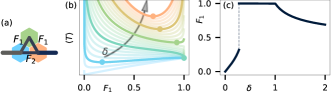
Figure 3: Phase transition in triangle geometry. (a) Triangle geometry. We consider $S_{\text{source}}=1=F_{1}+F_{2}$. (b) Value of $F_{1}$ obtained by minimising $\langle T\rangle$ for various scalings $\delta$. There is a discontinuous transition at $\delta\approx 0.275$ and a continuous transition at $\delta=1$. (c) Energy ($\langle T\rangle$) landscape for various $\delta$. Circles indicate select minima.

For blood vessels each edge corresponds to a tube of a given radius $r_{e}$. We can thus relate $F_{e}\sim v_{e}r_{e}^{2}$, where $v_{e}$ is the fluid velocity along the tube. Furthermore, in Poiseuille flow $C_{e}\sim r_{e}^{4}$, and thus $T_{ij}=T_{e}=L_{e}/v_{e}\sim L_{e}\sqrt{C_{e}}/F_{e}$. This shows that the time travelling across an edge is minimised by having a small conductivity, since in small tubes the liquid will have to move faster for the same flux $F$. So while we are interested in solutions that minimise time, this formulation yields solutions that are severely dissipation inefficient in which case power optimisation becomes more relevant than time minimisation. Instead, we reformulate $T_{ij}$ in terms of only the flows $F$ such that we stay in reasonably power-efficient regimes, as established by Eq. (4). Taking $\gamma=1$, we have

$$T_{ij}\sim\frac{L_{ij}}{\sqrt{|F_{ij}|}},$$ (7)

which is the definition we will use, and critically what enables the optimisation problem to yield non-trivial results. Variations induced by different values of $\gamma$ also work, as will be shown. We thus minimise the average time $\langle T\rangle$ in the regime where large fluid flows are associated with large conductivities. Equations (5–7) define the optimisation problem, which we solve by a momentum-based version of gradient descent Note2 .

Periphery-center optima — The result of our minimisation scheme is shown in Fig. 2c. First we note that the single-source-sink system prevents self-similar branching solutions that are known from single-source, multiple-sink systems. Instead the solution only has a few main branches, in particular one at the periphery and one at the center. Interestingly, this exact pattern is one of the three topologies [Fig. 1(a-c)] of pancreatic islet blood flow observed in nature Nyman2008 ; El-gohary2018 .

In some species, such as rodents, the glucagon-producing alpha cells and the insulin-producing beta cells comprising the islets are heterogeneously distributed with the beta cells in the center and alpha cells at the periphery. It has thus been suggested that the order of the flow suggests intercellular communication and regulation Nyman2008 , i.e. beta cells regulating alpha cells or vice versa, depending on the flow topology. Our results show a separate, but non-exclusive explanation that the patterns can appear due to an optimisation of the flow itself, independent of any heterogeneous distribution of cells. Interpreted in an evolutionary sense, one could imagine that optima such as the one derived here led to the present flow topology before the advent of alpha and beta cells and thus drove the heterogeneous distribution thereof.

The equal distribution of flow to each node and the sparsity of the network in the optimum [Fig. 2c] is possible due to the scaling of Eq. (7). In fact, considering instead $T_{ij}\sim L_{ij}/|F_{ij}|^{\delta}$ our model works for a broad range of $\delta$. To illustrate this, consider the simple network of three nodes shown in Fig. 3a. Taking $1=F_{1}+F_{2}$ it follows that $2\langle T\rangle=(1-F_{1})^{1-\delta}+2F_{1}^{1-\delta}+F_{1}^{-\delta}$, which is shown in Fig. 3b for various values of $\delta$. Minimising $\langle T\rangle$, the optimal $F_{1}$ is shown in Fig. 3c, which demonstrates that this system has a discontinuous phase transition at $\delta\approx 0.275$ and a continuous phase transition at $\delta=1$ in $F_{1}$. Between these values the optimal $F_{1}$ is independent of $\delta$, which is the regime we study.

The discontinuous phase transition occurs because the left and top node of Fig. 3a have conflicting optima: the left node minimises its time by having $F_{2}$ large, whereas the top node needs $F_{1}$ large. Large $\delta$ favour large $F_{1}$ because then a larger flow velocity compensates for the larger length of the upper branch. In contrast, a small $\delta$ favours the shorter path of the lower branch, while only leaving a small flux through the upper branch required to transport the product from the top node.

For more complex graphs such as the one we consider [Fig. 1e], the phase transition behaviour is much more rich and complex and the discontinuous transition is pushed to lower values, and the continuous transition happens at a $\delta$ smaller than (but close to) 1. Our choice of $\delta=\nicefrac{{1}}{{2}}$ lies safely within the regime, where the results are independent of the precise value of $\delta$ and where the resulting networks are sparse graphs. Thus our results are to a large degree independent of the scaling in Eq. (7).

The left-right asymmetry and thus the periphery-to-center flow of Fig. 2c comes from the fact that we are minimising the time for the product to reach the outlet from the nodes. The large collection branch emerging from the center thus minimises the time for many nodes by providing a fast route. Had we instead minimised the time from the source to the nodes $\langle T_{r}\rangle$ the solution would be reversed, since it would be important to reach the nodes fast. Indeed this opposite situation, with flow from center to periphery, is the most commonly observed topology in rodents Nyman2008 , and could perhaps hint that the time for “information” (e.g. glucose levels) to reach the cells is more important than the product to exit the islet.

Naturally, the combination of time from inlet to nodes and from nodes to outlet $\langle T_{c}\rangle=(1-\alpha)\,\langle T\rangle+\alpha\,\langle T_{r}\rangle$ ($0\leq\alpha\leq 1$) can also be optimised over. Fig. 4 shows examples of minimising $\langle T_{c}\rangle$. $\alpha=0$ corresponds to situation we have already studied, and $\alpha=1$ simply left-right mirrors this solution. In-between a compromise of the two optima is reached, e.g. as shown for $\alpha=0.25$ in Fig. 4a. The value of $\langle T_{c}\rangle$ is minimised for $\alpha=0$ and $\alpha=1$, since for any other value the solution will be the average of two solutions that both compromise. At precisely $\alpha=0.5$ the solution becomes left-right symmetric [Fig. 4b] yielding an islet topology similar to that of Fig. 1b.

Minimal flow constraints — While the solution of Fig. 2c does indeed distribute the flow to all nodes, some nodes see much more fluid flowing through them than others. As the pancreatic islets grow and if the blood flow source cannot keep up with this growth, each cell/node will see a decrease in flow permeating them. In this way, growth in networks flows can be emulated by a decreasing $S_{\text{source}}$ Ronellenfitsch2016 . At the same time a minimum amount of flow might be required at each cell e.g. for accurate estimation of glucose levels. This leads us to consider adding minimal flow constraints to the optimisation problem.

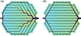
Figure 4: Varying the ratio $\alpha$ between time from nodes to outlet and inlet to nodes. (a) Obtained optimum at $\alpha=0.25$. (b) The left-right symmetric solution obtained at $\alpha=0.5$.

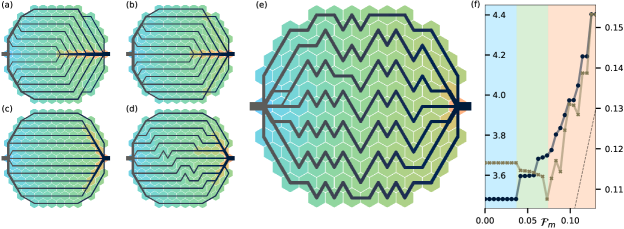
Figure 5: Optimal graphs under minimal flow constraints. (a) At $\mathcal{F}_{m}=0.042$, the network of Fig. 2c loses its front collection channels. (b) The collection point starts moving to the right as $\mathcal{F}_{m}$ is increased to $0.062$. (c) At $\mathcal{F}_{m}=0.073$ the collection point has moved to the far right. (d) One horizontal vessel has been removed by introducing kinks at $\mathcal{F}=0.078$ which increases the flow in the remaining vessels. (e) Buckling increases; $\mathcal{F}_{m}=0.125$. As $\mathcal{F}_{m}\rightarrow 1$ the global optimum becomes a Hamiltonian path through the nodes. (f) In dark blue (left axis) the average time $\langle T\rangle$ is shown as function of $\mathcal{F}_{m}$. The average flow through the nodes $\langle\mathcal{F}\rangle$ is shown in light brown (right axis). Dashed line shows $f(x)=x$, which matches the slope of $\langle\mathcal{F}\rangle$ in the buckling section. Background colours denote section: global optimum in blue, unbuckled solution in green, and buckled in red.

The flow through a node $i$ with $S_{i}=0$ is

$$\mathcal{F}=\sum_{j\in\mathcal{O}_{i}}|F_{ij}|=\sum_{j\in\mathcal{I}_{i}}|F_{ij}|$$ (8)

and we now require $\mathcal{F}\geq\mathcal{F}_{m}$ for all nodes for a given value of $\mathcal{F}_{m}$. Obtained minima are shown in Fig. 5 under variations of $\mathcal{F}_{m}$.

The optimal configuration of Fig. 2c has $\min_{i}\mathcal{F}=0.041$ and thus for any $\mathcal{F}_{m}$ smaller than this the same solution is obtained (blue section in Fig. 5f). As $\mathcal{F}_{m}$ is increased above this, the network adapts to more equally divide the flow. First the two middle branches are lost [Fig. 5a] and then the collection point starts moving towards the outlet [Fig. 5b]. In the end of this process (green section in Fig. 5f), the collection branch has moved all the way to the right [Fig. 5c]. As can be seen in Fig. 5f, naturally, the average time $\langle T\rangle$ increases as $\mathcal{F}_{m}$ increases. Fig. 5f also shows that $\langle\mathcal{F}\rangle_{i}$ decreases rapidly. So as this reordering occurs, the minimum flow rate increases at the expense of the average flow rate.

As $\mathcal{F}_{m}$ is increased further than reordering can accomodate for, buckling occurs [Fig. 5d], the degree of which increases as $\mathcal{F}_{m}$ is increased [Fig. 5e]. As soon as buckling occurs, $\langle\mathcal{F}\rangle$ starts increasing as seen in Fig. 5f. This increase scales linearly with $\mathcal{F}_{m}$, i.e. the average flow rate, after buckling, stays at a fixed level above $\mathcal{F}_{m}$. We note that the noise in $\langle\mathcal{F}\rangle$ in Fig. 5f most likely indicates that our optimisation scheme in some cases fails to find the true global optimum but ends in neighbouring local minima.

As shown in Fig. 1d, pancreatic islets do indeed have a severely tortuous vasculature Berclaz2016 similar to that obtained in Fig. 5. The mechanical reason for buckling in real islets could be due to growth-induced buckling Kirkegaard2019 . Our analysis shows how such buckling could actually be of benefit to the system under growth.

In comparing our result with blood vessels in pancreatic islets, we implicitly assume that transport time is of main concern. In fact the average blood flow velocity in Langerhans islets is $\sim 1.4$ mm/s Berclaz2016 , implying that transport across an islet takes about $\sim 0.5$ second. Activity of both alpha and beta cells are pulsatile, and in-vitro experiments show coherent oscillations of whole islets with periods down to three seconds Valdeolmillos1989 . In order for the organism to utilize coherent release of insulin downstream of islets, it is therefore plausible that time optimization on the sub-second scale is functional.

In conclusion, by simply varying how much time to nodes and time from nodes is important through the parameter $\alpha$, our proposed optimisation problem on network flows directly leads to flow topologies similar to those observed in real pancreatic islet and illustrated in Fig. 1(a-c). We have furthermore shown how minimum flow constraints leads to buckling and thus tortuous vessels as found in real islets. Our approach applies generally to all laminar network flows that have single-source and single-sink characteristics.

- (1) Steffen Bohn and Marcelo O. Magnasco. Structure, scaling, and phase transition in the optimal transport network. Physical Review Letters, 98(8):3–6, 2007.
- (2) Dan Hu and David Cai. Adaptation and optimization of biological transport networks. Physical Review Letters, 111(13):1–5, 2013.
- (3) Henrik Ronellenfitsch and Eleni Katifori. Global Optimization, Local Adaptation, and the Role of Growth in Distribution Networks. Physical Review Letters, 117(13):1–5, 2016.
- (4) Eleni Katifori, Gergely J. Szöllosi, and Marcelo O. Magnasco. Damage and fluctuations induce loops in optimal transport networks. Physical Review Letters, 104(4):1–4, 2010.
- (5) Francis Corson. Fluctuations and redundancy in optimal transport networks. Physical Review Letters, 104(4):1–4, 2010.
- (6) Peter Sheridan Dodds. Optimal form of branching supply and collection networks. Physical Review Letters, 104(4):1–4, 2010.
- (7) Parviz M. Pour, Jens Standop, and Surinder K. Batra. Are islet cells the gatekeepers of the pancreas? Pancreatology, 2(5):440–448, 2002.
- (8) Hyunsuk Hong, Junghyo Jo, and Sang Jin Sin. Stable and flexible system for glucose homeostasis. Physical Review E - Statistical, Nonlinear, and Soft Matter Physics, 88(3):1–6, 2013.
- (9) Corinne Berclaz, Daniel Szlag, David Nguyen, Jérôme Extermann, Arno Bouwens, Paul J. Marchand, Julia Nilsson, Anja Schmidt-Christensen, Dan Holmberg, Anne Grapin-Botton, and Theo Lasser. Label-free fast 3D coherent imaging reveals pancreatic islet micro-vascularization and dynamic blood flow. Biomedical Optics Express, 7(11):4569, 2016.
- (10) Hiroaki Shimokawa. The Order of Islet Microvascular Cellular Perfusion Is B—-A—-D in the perfused rat pancreas. Journal of Clinical Investigation, 82(1):350–353, 1988.
- (11) Lara R. Nyman, K. Sam Wells, W. Steve Head, Michael McCaughey, Eric Ford, Marcela Brissova, David W. Piston, and Alvin C. Powers. Real-time, multidimensional in vivo imaging used to investigate blood flow in mouse pancreatic islets. Journal of Clinical Investigation, 118(11):3790–3797, 2008.
- (12) Yousef El-gohary and George Gittes. Structure of Islets and Vascular Relationship to the Exocrine Pancreas. Pancreapedia, 2017.
- (13) Julius B. Kirkegaard, Bjarke F. Nielsen, Ala Trusina, and Kim Sneppen. Self-assembly, Buckling & Density-Invariant Growth of Three-dimensional Vascular Networks. Journal of the Royal Society Interface (in press), arXiv preprint:1910.01949, 2019.
- (14) Briefly, minimising under constant by the method of Lagrange multipliers leads to from which the scaling follows. See e.g. Ref. Bohn2007 for details.
- (15) See supplemental information, which cites Golub1973 .
- (16) GH Golub and V Pereyra. The differentiation of pseudo-inverses and nonlinear least squares problems whose variables seperate. SIAM Journal on Numerical Analysis, 10(2):283–289, 1973.
- (17) Miguel Valdeolmillos, Rosa M. Santos, Diego Contreras, Bernat Soria, and Luis M. Rosario. Glucose-induced oscillations of intracellular Ca2+ concentration resembling bursting electrical activity in single mouse islets of Langerhans. FEBS Letters, 259(1):19–23, 1989.