Parameter space arrangement
for a model system nearby domain of existence
of Plykin type attractor

Abstract

For a model system defined as combination of sequentially applied continuous transformations of a sphere, the question of arrangement of the parameter space around the domain of existence of the Plykin-type attractor is considered. Results of numerical calculations are presented, including charts of dynamical regimes and Lyapunov exponents on the parameter plane, as well as portraits of attractors in characteristic regions of chaotic and regular dynamics. The Plykin attractor region is determined and depicted using the computational procedure for checking hyperbolicity, which consists in analyzing angles between expanding and contracting tangent subspaces of typical trajectories on the attractor. The Plykin attractor takes place in a bounded continuous region of the parameter plane that corresponds to roughness (structural stability) of the hyperbolic dynamics. Outside that region, various types of dynamics are observed including non-hyperbolic chaos, periodic and quasiperiodic behaviors.

Keywords— hyperbolic chaos, Plykin attractor, Lyapunov exponent, structural stability, parameter space, scenarios of transition to chaos

Uniformly hyperbolic attractors introduced in the second half of the 20th century in a framework of rigorous mathematical theory provide examples of strictly justified deterministic chaos in dynamical systems [1,2,3]. These are attractors consisting exclusively of saddle-type phase trajectories, so that each trajectory has stable and unstable manifolds formed by sets of neighboring orbits approaching or moving away from the reference trajectory.

Until recently, only artificial mathematical constructions like Smale–Williams solenoid and Plykin attractor were considered as examples of the uniformly hyperbolic attractors. The Smale–Williams attractor appears while mapping a toroidal domain in the phase space of minimal dimension 3 with longitudional expansion and transversal contracting into itself been being rolled up into a multi-turn loop. The Plykin attractor [4,5] can be realized for a map on a sphere with four holes, or in a bounded region on a plane with three holes.

A fundamental mathematical fact is that the hyperbolic chaos has the property of roughness, or structural stability, which consists in the fact that it exhibits dynamics, which do not change qualitatively under a small variation of parameters [6]. This property would be of exceptional importance for natural systems and for technical applications, providing insensitivity of chaos characteristics to inaccurate parameter settings, manufacturing errors, various noises and disturbances.

Recently, examples of systems admitting a physical realization have been proposed, where the Smale–Williams or Plykin hyperbolic attractors take place for the mappings, which arise when constructing the Poincaré sections [7].

A fundamentally important question in the search, design, and use of systems with hyperbolic chaos is how the dynamics depend on parameters in regions where occurrence of such chaos is potentially possible. Theoretically, this is valuable for enriching mathematical concepts, as a step from considering rough situations to situations of varying degrees of non-roughness, like in the traditional theory of bifurcations. Practically, this is important for optimizing characteristics of the designed chaos generators. Also, information about the arrangement of the parameter space surrounding the area of hyperbolic chaos can help in the search for systems of natural origin, which manifest the hyperbolic dynamics (mechanics, neurodynamics, chemical kinetics, etc.).

By virtue of roughness, hyperbolic chaos must occupy continuous domains in the parameter space, but the environment structure of these regions is of interest as characterizing bifurcation scenarios of transition to the hyperbolic chaos. The available literature on this issue so far refers only to the simplest type of hyperbolic attractors, namely, the Smale–Williams solenoids [9, 10, 11, 12].

This article discusses arrangement of the parameter space region surrounding the area of existence of the Plykin attractor in the model system [8]. The system is constructed using a certain periodic sequence of continuous transformations of the sphere. To make the task more meaningful, we first modify the model, supplementing it with parameters, depending on which the analysis of dynamical behavior will be conducted. Further, we present results of computations, including visualization of charts of dynamical regimes and Lyapunov exponents on the parameter plane, as well as attractor portraits in characteristic regions of chaotic and regular dynamics. In a frame of these studies, the region of existence of the Plykin hyperbolic attractor is determined using the special computational procedure for checking hyperbolicity, based on the analysis of angles between the expanding and contracting tangent subspaces of typical trajectories on the attractor [15-17].

1 The model system

Following [8], we assume that for our system instantaneous states are given by points of the unit sphere, which can be represented in angular coordinates $(\theta,\,\varphi)$ or in rectangular coordinates $(x,\,y,z)$:

$$x=\cos\varphi\sin\theta,\quad y=\,\sin\varphi\sin\theta,\quad z=\cos\theta,$$ (1)

where $x^{2}+y^{2}+z^{2}=1$ (Fig.1). As proved by Plykin, a map of a sphere onto itself can have a hyperbolic attractor only in presence of at least four holes, the regions not visited by trajectories on the attractor. In our construction the holes correspond to neighborhoods of the points A, B, C, D with coordinates $(x,y,z)=(\pm 1/\sqrt{2},\,\,0,\,\,\pm 1/\sqrt{2})$, see Fig.1. The North and South poles of the sphere are denoted as N and S, respectively.

Let us consider a sequence of four continuous transformations:

I. Displacement of representative points per unit time along the parallels from the meridians NABS and NCDS towards the meridian circle equidistant from them:

$$\dot{x}=-\varepsilon xy^{2},\,\,\,\dot{y}=\varepsilon x^{2}y,\,\,\,\,\dot{z}=0.$$ (2)

II. Differential rotation per time $T_{1}$ around $z$ axis with angular velocity linearly dependent on $z$:

$$\dot{x}=\pi(z/\sqrt{2}+1/2)y,\,\,\,\,\dot{y}=-\pi(z/\sqrt{2}+1/2)x,\,\,\,\,\dot{z}=0.$$ (3)

III. Displacement of representative points per unit time on the sphere along circles with centers at the axis $x$ from a large circle ABCD towards the equator:

$$\dot{x}=0,\,\,\,\dot{y}=\varepsilon yz^{2},\,\,\,\dot{z}=-\varepsilon y^{2}z.$$ (4)

IV. Differential rotation per time $T_{2}$ around $x$ axis with angular velocity linearly dependent on $x$:

$$\dot{x}=0,\,\,\,\dot{y}=-\pi(x/\sqrt{2}+1/2)z,\,\,\,\dot{z}=\pi(x/\sqrt{2}+1/2)y.$$ (5)

Unlike the previously considered model, the durations of the stages II and IV are considered as parameters, depending on which the dynamical behavior analysis will be carried out, whereas in [8] they were fixed ($T_{1}=T_{2}$=1).

The Poincaré map ${\rm{\bf x}}\mapsto{\rm{\bf F(x)}}$ describing evolution of the system over a period $T=2+T_{1}+T_{2}$ is the result of sequential application of four mappings, corresponding to the stages I-IV, to the initial state ${\rm{\bf x}}=(x,y,z)$:

$${\rm{\bf x}}\mapsto\left({\begin{array}[]{l}x\sqrt{\frac{x^{2}+y^{2}}{x^{2}+y^{2}e^{2\varepsilon(x^{2}+y^{2})}}},\\ y\sqrt{\frac{x^{2}+y^{2}}{x^{2}e^{-2\varepsilon(x^{2}+y^{2})}+y^{2}}},\\ \,z\\ \end{array}}\right),$$

$${\rm{\bf x}}\mapsto\left({\begin{array}[]{l}x\cos\frac{\pi T_{1}(z\sqrt{2}+1)}{2}+y\sin\frac{\pi T_{1}(z\sqrt{2}+1)}{2},\\ -x\sin\frac{\pi T_{1}(z\sqrt{2}+1)}{2}+y\cos\frac{\pi T_{1}(z\sqrt{2}+1)}{2},\\ z\\ \end{array}}\right),$$

$${\rm{\bf x}}\mapsto\left({\begin{array}[]{l}x,\\ y\sqrt{\frac{z^{2}+y^{2}}{z^{2}e^{-2\varepsilon(z^{2}+y^{2})}+y^{2}}},\\ z\sqrt{\frac{z^{2}+y^{2}}{z^{2}+y^{2}e^{2\varepsilon(z^{2}+y^{2})}}}\\ \end{array}}\right),$$

$${\rm{\bf x}}\mapsto\left({\begin{array}[]{l}x,\\ y\cos\frac{\pi T_{2}(x\sqrt{2}+1)}{2}-z\sin\frac{\pi T_{2}(x\sqrt{2}+1)}{2},\\ y\sin\frac{\pi T_{2}(x\sqrt{2}+1)}{2}+z\cos\frac{\pi T_{2}(x\sqrt{2}+1)}{2}\\ \end{array}}\right).$$ (6)

2 Plykin attractor and method for validating the hyperbolicity

We first set the fixed $T_{1}=T_{2}$=1, which, with a suitable choice of $\varepsilon$, say, $\varepsilon=0.77$, ensures, according to [8], occurrence of the Plykin attractor. Fig. 1 shows a phase portrait of the attractor in axonometric projection obtained from results of numerical calculations by iterations of the mapping ${\rm{\bf x}}\mapsto{\rm{\bf F(x)}}$.

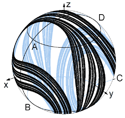
Figure 1: Attractor of the mapping (6) at $\varepsilon$=0.77 on the unit sphere

The description of the dynamics can be reformulated in such way that the instantaneous states of the system are represented by points on a plane. A suitable replacement of the variables is

$$W=X+iY=\frac{x-z+iy\sqrt{2}}{x+z+\sqrt{2}},$$ (7)

which corresponds to a stereographic projection from the sphere onto the plane when taking a point C$(-1/\sqrt{2},\,\,0,\,\,-1/\sqrt{2})$ as the center of the projection. This point does not belong to the attractor (it is in the “hole”), therefore, the attractor obtained by the variable change (7) occupies a bounded area on the plane. The portrait of the attractor on the plane is shown in Fig.2a. We note the presence of a specific fractal transverse structure: the object looks like consisting of stripes, each of which is composed of narrower stripes and so on.

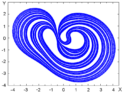
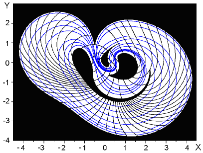
Figure 2: Portrait of the attractor for the mapping ${\rm{\bf x}}\mapsto{\rm{\bf F(x)}}$ at $\varepsilon$=0.77, $T_{1}$=$T_{2}$=1 depicted on the plane (a). Stable and unstable foliations in the attractor absorbing area shown in white, which are visualized from the results of computations (b).

To make sure that the attractor is hyperbolic, stable and unstable foliations in the region containing the attractor are visualized in Fig. 2b. Stable and unstable manifolds are shown, respectively, in black and blue. As seen from the figure, unstable manifolds follow the attractor fibers, and stable manifolds are located across them. The mutual disposition of the stable and unstable manifolds in the region containing the attractor definitely excludes tangencies.

The Lyapunov exponents calculated for this attractor via the standard algorithm, which uses iterations along the reference trajectory of two sets of linearized equations accompanied with the Gram–Schmidt orthogonalization [13], are

$$\Lambda_{1}=0.9587,\,\,\,\Lambda_{2}=-1.1407.$$ (8)

The presence of a positive exponent indicates chaotic nature of the attractor. The Kaplan–Yorke dimension of the attractor, which is determined via the Lyapunov exponents, is $D_{KY}\approx$1.84. It serves as a quantitative expression of the fractal structure of the bands forming the attractor as observed in Figures 1 and 2.

One of the conventional computer tests for hyperbolicity consists in calculating small perturbation vectors along a reference orbit on the attractor during forward and backward evolution in time with evaluating the angles between the vector subspaces responsible for instability [14,15,16]. If the statistical distribution of these angles is separated from zero angles, then the dynamics is diagnosed as hyperbolic. In our case, the subspaces of instability in direct time and in reverse time are one-dimensional.

The procedure begins with calculating a rather long phase trajectory on the attractor by iterations of the map. Further, the linearized equations are solved forward in time along the reference trajectory with normalization of the resulting vectors ${\rm{\bf a}}_{n}$ at the end of each switching period. This vector determines the unstable direction at the points of the orbit generated by the map. Further, along the same trajectory, linearized equations are solved backward in time, from which the vectors ${\rm{\bf b}}_{n}$ are obtained. Then, for each $n$, one calculates the angle between the vectors ${\rm{\bf a}}_{n}$ and ${\rm{\bf b}}_{n}$, using the formula $\cos\alpha_{n}={\left|{{\rm{\bf b}}_{n}\cdot{\rm{\bf a}}_{n}}\right|}\mathord{\left/{\vphantom{{\left|{{\rm{\bf b}}_{n}\cdot{\rm{\bf a}}_{n}}\right|}{|{\rm{\bf b}}_{n}||{\rm{\bf a}}_{n}|}}}\right.\kern-1.2pt}{|{\rm{\bf b}}_{n}||{\rm{\bf a}}_{n}|}$.

Figure 3 shows a histogram of the angles obtained for system (6) at $\varepsilon$=0.77, $T_{1}=T_{2}=1$. It is clearly seen that the distribution does not contain angles close to zero, which indicates the hyperbolic nature of the attractor.

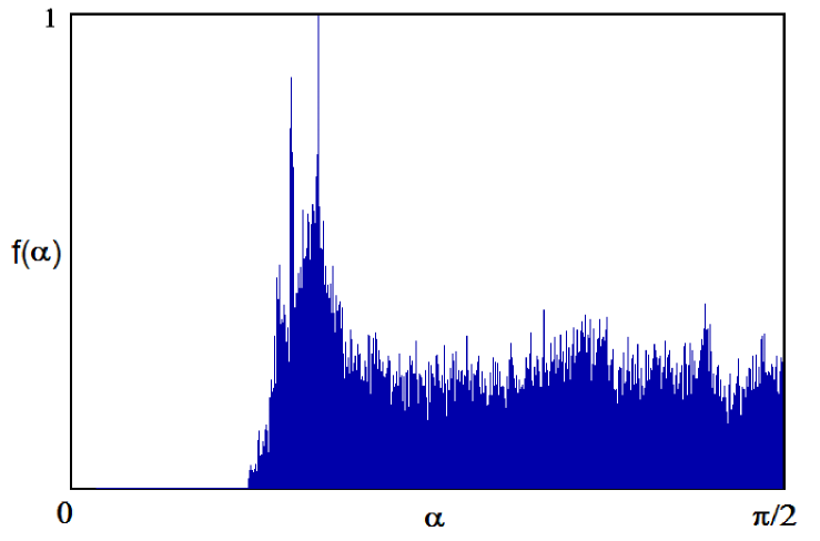
Figure 3: Histogram of the distribution of angles $\alpha$ between the subspaces of the perturbation vectors corresponding to instabilities in the forward and reverse time along a reference orbit on the attractor, obtained according to the method explained in the text.

3 Charts of dynamical regimes. Chaotic and regular attractors

To plot a chart of dynamical regimes, the parameter plane is scanned by going through the grid nodes with a certain step in two parameters (see, for example, [14, 18]). At each point, about $10^{3}$ iterations of the mapping ${\rm{\bf x}}\mapsto{\rm{\bf F(x)}}$ are performed, and according to the results of the last iteration steps, an analysis is carried out for the presence of a repetition period from 1 to 14 with some given level of allowable error. If periodicity is detected, the corresponding pixel in the diagram is indicated by a certain color, and the procedure continues with analysis of the next point on the parameter plane. Similarly, the color coding may be used not for the periods, but for the value of the largest Lyapunov exponent; then we get a representation of the parameter plane as a Lyapunov chart [19, 14]. Figure 4 demonstrates a chart of regimes on the plane ($T_{1}$, $T_{2})$ for $\varepsilon$ = 0.77, on which, in addition to periodic modes encoded with the corresponding colors, the areas of quasiperiodicity (black color), chaos (white), and hyperbolic chaos (red color, with the letter H) are shown.

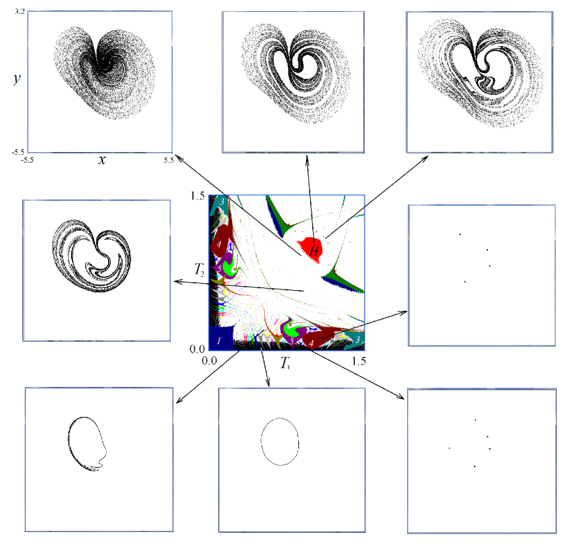
Figure 4: In the center is the chart of regimes for $\varepsilon=0.77$. Black corresponds to quasiperiodic modes, white corresponds to chaotic ones, and other colors designate periodic modes. For the main periodic tongues the periods are indicated by numbers. The region of existence of the hyperbolic chaotic attractor is shown in red and marked additionally with the letter H. The margin pictures show representative phase portraits of attractors for some particular points on the parameter plane.

The chart is symmetrical with respect to the diagonal, i.e., with respect to the replacement of the parameters $T_{1}\leftrightarrow T_{2}$, which is natural given the structure of the equations (6).

The hyperbolic attractor and periodic regimes occupy solid areas; this fact is associated with their roughness.

Departure for a small distance in one or another direction from the region of hyperbolic chaos leaves the attractor chaotic, but it becomes non-hyperbolic.

Figure 5a shows graphs of the dependences of Lyapunov exponents on a parameter counted along the main diagonal on the chart of Fig. 4. When leaving the region of hyperbolicity in the diagonal direction up to the right, the fibers forming the structure of the attractor undergo deformation, but no visible broadening occurs, and the fractal band-in-band structure is locally preserved. The Lyapunov exponents vary little in the region of hyperbolicity, and the Kaplan–Yorke dimension remains greater than 1 and noticeably less than 2. The graphs for the Lyapunov dimension along the diagonal are shown in Figure 5b.

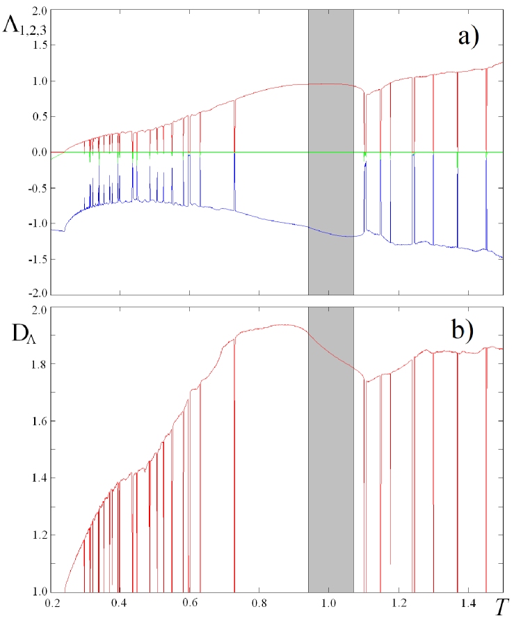
Figure 5: Dependencies of the Lyapunov exponents (a) and of the Lyapunov dimension (b) on the parameter $T=T_{1}=T_{2}$, which is counted along the main diagonal on the chart of Fig. 4. Gray tone indicates the region of hyperbolicity of the attractor.

When going diagonally to the left down, the situation looks different, namely, as “closing the holes”, which were ensuring the existence of the Plykin attractor, while the bands that make up the structure of the attractor undergo broadening, close together, merge, and the fractal structure fade away. The fractality disappearance is also evidenced by the fact that the two Lyapunov exponents become close in absolute value, which means that the Kaplan–Yorke dimension of the attractor is approaching 2.

On the parameter plane, in a strip along the vertical axis (small $T_{1}$ values) and in a strip along the horizontal axis (small $T_{2}$ values), i.e. where the duration of one stage of the differential rotation is much shorter than the other, one can see a characteristic picture of the Arnold synchronization tongues [20, 14] corresponding to periodic regimes of different periods. Between tongues there are areas of quasiperiodic dynamics. An exit from each tongue along the path inside it in the direction of expanding the tongue (i.e., up for the set of tongues in the bottom part of the chart, or right for the tongues in the left part of the diagram) is accompanied by period doubling bifurcations with transition to non-hyperbolic chaos according to the Feigenbaum scenario [21,14].

The regions of non-hyperbolic chaos between the Arnold tongues and the Plykin attractor have inclusions in a form of “shrimps” [22,23], where periodic dynamics is restored. This is characteristic of a fragile chaos situation associated with the mathematical concept of a quasiattractor [3], which occur in many other chaotic systems studied in the literature (Hénon map, Rössler model, etc.).

Figures 6 and 7 show charts for other two-dimensional sections of the three-dimensional parameter space of the system (6). Inspection of these charts shows that the region of the hyperbolic attractor is bounded from above in the parameter $\varepsilon$. With increase of $\varepsilon$, the system manifests a developed multistability.

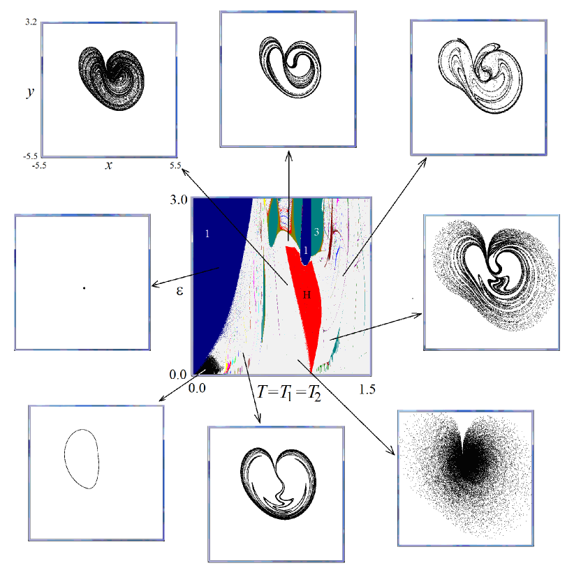
Figure 6: In the center is the chart of regimes on the parameter plane ($T=T_{1}=T_{2}$, $\varepsilon)$. Black corresponds to quasiperiodic modes, white corresponds to chaotic ones, and other colors designate periodic modes. For the main periodic tongues the periods are indicated by numbers. The region of existence of the hyperbolic chaotic attractor is shown in red and marked with the letter H. The margin pictures show representative phase portraits of attractors for some particular points on the parameter plane.

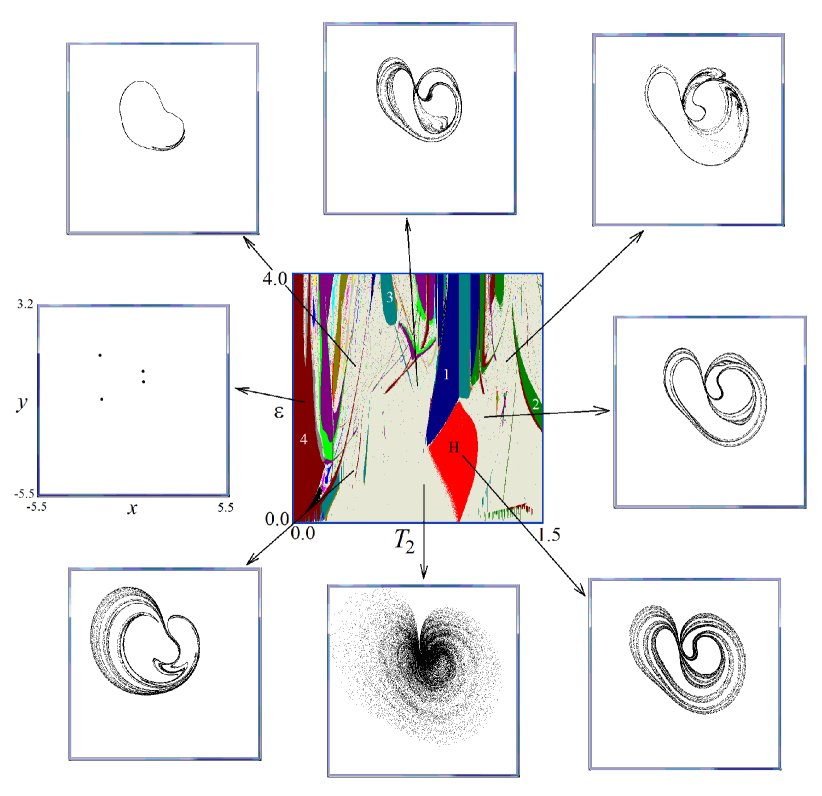
Figure 7: In the center is the chart of regimes on the parameter plane ($T_{2}$, $\varepsilon)$ at $T_{1}=1$. Black corresponds to quasiperiodic modes, white corresponds to chaotic ones, and other colors designate periodic modes. For the main periodic tongues the periods are indicated by numbers. The region of existence of the hyperbolic chaotic attractor is shown in red and marked with the letter H. The margin pictures show representative phase portraits of attractors for some particular points on the parameter plane.

4 Conclusions

We have considered a model system with Plykin type hyperbolic chaotic attractor in a map resulting from several successive transformations of a sphere such as differential rotations around two orthogonal axes alternating with stages of dissipative evolution. The attractor can also be considered on a plane by applying a stereographic projection.

The dependence of the dynamical behavior of the system on parameters specifying the duration of the stages of differential rotation and the dissipation parameter is discussed. Charts of dynamical regimes are presented, which make it possible to judge about mutual location of the regions of periodic, quasiperiodic, chaotic, and hyperbolic chaotic behavior in the parameter space of the system.

It is shown that the hyperbolic attractor and the periodic modes occupy solid regions in the parameter space, which is obviously due to the roughness of the corresponding types of dynamical behavior.

Upon leaving the periodicity regions, scenarios of transition to quasiperiodicity and chaos known in nonlinear dynamics occur, which correspond to the structures in the form of Arnold tongues in the parameter space. When leaving the hyperbolic chaos region of for a short distance, the attractor remains chaotic, but becomes non-hyperbolic. Two scenarios stand out qualitatively depending on the direction of the exit. One corresponds to a situation that the fibers forming the attractor structure undergo deformation, but without their visible broadening, and the “strip in strip” fractal structure is locally preserved. The second scenario looks like “closing the holes” which were ensuring existence of the Plykin attractor, when the bands that make up the structure of the attractor undergo broadening, and the attractor loses its fractal structure. The region of non-hyperbolic chaos manifests inclusions in the form of “shrimps”, where periodic dynamics is restored that is typical for non-rough chaos.

Summarizing, the first qualitative information on the parameter space arrangement around the region of the Plykin attractor has been obtained. It is of obvious interest to continue researches in this direction to identify details of the bifurcation transitions, to construct a complete classification of the scenarios of birth and destruction of hyperbolic chaos, and to develop comparative analysis of the pictures of the parameter spaces near the regions of occurrence of different types of uniformly hyperbolic attractors.

References

- [1]
- [2] Anosov, D.V., Gould, G.G., Aranson, S.K., Grines, V.Z., Plykin, R.V., Safonov, A.V., Sataev, E.A., Shlyachkov, S.V., Solodov, V.V., Starkov, A.N., Stepin, A.M. Dynamical Systems IX: Dynamical Systems with Hyperbolic Behaviour. Encyclopaedia of Mathematical Sciences, 1995, v. 9. (Springer).
- [3] Katok, A. and Hasselblatt, B., Introduction to the Modern Theory of Dynamical Systems, Cambridge: Cambridge University Press, 1996.
- [4] Shilnikov L. Mathematical Problems of Nonlinear Dynamics: A Tutorial. International Journal of Bifurcation and Chaos in Applied Sciences and Engineering, 1997, 7, 1353-2001.
- [5] Plykin, R.V. Sources and sinks of A-diffeomorphisms of surfaces. Math. USSR-Sb., 1974, 23(2), 233-253.
- [6] Guckenheimer, J. and Holmes, P.J. Nonlinear Oscillations, Dynamical Systems, and Bifurcations of Vector Fields. Springer, 1983.
- [7] Pugh, C., Peixoto, M.M. Structural stability. Scholarpedia, 2008, 3 (9):4008.
- [8] Kuznetsov, S.P. Dynamical chaos and uniformly hyperbolic attractors: from mathematics to physics. Physics-Uspekhi, 2011, 54 (2), 119-144.
- [9] Kuznetsov, S.P. A non-autonomous flow system with Plykin type attractor. Communications in Nonlinear Science and Numerical Simulation, 2009, 14, 3487-3491.
- [10] Shil’nikov, L.P., Turaev, D.V. Simple bifurcations leading to hyperbolic attractors. Computers & Mathematics with Applications, 1997, 34 (2-4), 173-193.
- [11] Isaeva, O.B., Kuznetsov, S.P., Sataev, I.R. A “saddle-node” bifurcation scenario for birth or destruction of a Smale–Williams solenoid. Chaos, 2012, 22, 043111.
- [12] Isaeva, O.B., Kuznetsov, S.P., Sataev, I.R., Savin, D.V., Seleznev, E.P. Hyperbolic Chaos and Other Phenomena of Complex Dynamics Depending on Parameters in a Nonautonomous System of Two Alternately Activated Oscillators. International Journal of Bifurcation and Chaos in Applied Sciences and Engineering, 2015, 25, 1530033.
- [13] Kuptsov, P.V., Kuznetsov, S.P., Stankevich, N.V. A Family of Models with Blue Sky Catastrophes of Different Classes. Regular and Chaotic Dynamics, 2017, 22, 551-565.
- [14] Pikovsky, A., Politi, A. Lyapunov exponents: a tool to explore complex dynamics. Cambridge University Press, 2016.
- [15] Kuznetsov, S.P. Dynamical chaos. Moscow: Fizmatlit, 2001. (In Russian.)
- [16] Lai, Y.C., Grebogi, C., Yorke, J.A., Kan, I. How often are chaotic saddles nonhyperbolic? Nonlinearity, 1993, 6, 779-797.
- [17] Anishchenko, V.S., Kopeikin, A.S., Kurths, J., Vadivasova, T.E., Strelkova, G.I. Studying hyperbolicity in chaotic systems. Physics Letters A, 2000, 270, 301-307.
- [18] Kuptsov, P.V. Fast numerical test of hyperbolic chaos. Phys. Rev. E, 2012, 85, 015203.
- [19] Kuznetsov, A.P., Kuznetsov, S.P., Sataev, I.R. and Chua, L.O. Multi-parameter criticality in Chua’s circuit at period-doubling transition to chaos. International Journal of Bifurcation and Chaos in Applied Sciences and Engineering, 1996, 6, 119-148.
- [20] Markus, M. and Hess, B. Lyapunov exponents of the logistic map with periodic forcing. Computers and Graphics, 1989, 13, 553-558.
- [21] Mettin, R., Parlitz, U., and Lauterborn, W. Bifurcation structure of the driven van der Pol oscillator. International Journal of Bifurcation and Chaos in Applied Sciences and Engineering, 1993, 3, 1529-1555.
- [22] Bohr, T., and Gunaratne, G. Scaling for supercritical circle-maps: Numerical investigation of the onset of bistability and period doubling. Physics Letters A, 1985, 113(2), 55-60.
- [23] Gallas, J.A. Dissecting shrimps: results for some one-dimensional physical models. Physica A: Statistical Mechanics and its Applications, 1994, 202(1-2), 196-223.
- [24] Stoop, R., Martignoli, S., Benner, P., Stoop, R. L., and Uwate, Y. Shrimps: occurrence, scaling and relevance. International Journal of Bifurcation and Chaos in Applied Sciences and Engineering, 2012, 22, 1230032.