Intelligent Reflecting Surface Aided Network: Power Control for Physical-Layer Broadcasting

Abstract

As a recently proposed idea for future wireless systems, intelligent reflecting surface (IRS) can assist communications between entities which do not have high-quality direct channels in between. Specifically, an IRS comprises many low-cost passive elements, each of which reflects the incident signal by incurring a phase change so that the reflected signals add coherently at the receiver. In this paper, for an IRS-aided wireless network, we study the problem of power control at the base station (BS) for physical-layer broadcasting under quality of service (QoS) constraints at mobile users, by jointly designing the transmit beamforming at the BS and the phase shifts of the IRS units. Furthermore, we derive a lower bound of the minimum transmit power at the BS to present the performance bound for optimization methods. Simulation results show that, the transmit power at the BS approaches the lower bound with the increase of the number of IRS units, and is much lower than that of the communication system without IRS.

I Introduction

Benefiting from various advanced technologies, the fifth-generation (5G) communications achieves great improvements in spectral efficiency, such as massive antennas deployment at the base station (BS) (i.e., massive multiple-input multiple-output), non-orthogonal multiple access, millimeter wave communications, and ultra-dense hetnets. However, these advanced technologies will introduce great mounts of energy consumption, resulting in the high complexity of hardware implementation, which brings great challenges for practical implementations [1]. For example, the ultra-dense HetNets mean that there are lots of BSs in the network, and the energy consumption scales up with respect to the number of BSs. The massive antenna arrays consist of active elements and transmit/recieve data, thus consuming energy expensively.

Intelligent reflecting surface. To improve the spectral efficiency and reduce the energy consumption, researchers are exploring new ideas for future wireless systems [2, 3, 4, 5]. Among theses ideas, intelligent reflecting surface (IRS) has been considered in several studies [6, 7, 8, 9, 10]. An IRS is a planar array consisting of many reflecting and nearly passive units. Each IRS unit is controlled by the BS remotely to change the phase of the incident signal, so that the signals at the receiver can add coherently. In other words, IRS intelligently adjusts the propagation conditions to improve communication quality between the BS and mobile users (MUs). Since each IRS unit only reflects signals in a passive way, instead of transmitting/receiving signals in an active way, the energy consumption is very low. In addition, due to the characteristics of lightweight and low profile, the IRS can be deployed on walls/building facades, and the channel model between the BS and the IRS is usually characterized as line of sight (LoS) [6].

Our contributions. To address the problem of power control at the BS for physical layer broadcasting under quality of service (QoS) constraints at the MUs in an IRS-aided network, we propose to employ the alternating optimization algorithm to jointly design the transmit beamforming at the BS and the IRS units. Furthermore, we derive the lower bound of the minimum transmit power for the broadcast setting to present the performance bound for optimization methods. Simulation results show that, for the broadcasting transmit pattern, the transmit power at the BS approaches the lower bound with the increase of the number of IRS units, and is much lower than that of the communication system without IRS.

Comparing this paper with [6, 7]. Recently, Wu and Zhang [6, 7] also considered downlink power control under QoS, with phase shifts of IRS units having continuous domains in [6] and discrete domains in [7]. The differences between our paper and [6, 7] are twofold. First, our paper considers the broadcast setting, while [6, 7] are for the unicast setting. Second, under the line of sight (LoS) channel model between the BS and IRS, we analyze a lower bound of the minimum transmit power in the general setting (i.e., an arbitrary number of antennas at the BS, an arbitrary number of IRS units, and an arbitrary number of MUs), while [6, 7] only derived the relationship between the transmit power and the received power in the special setting of considering single user and single-antenna BS, ignoring the channel between BS and MU, and assuming that the channel model between the BS and IRS is Rayleigh fading.

Other related work. For IRS-aided wireless communications, in addition to [6, 7] above and [6]’s conference version [11] for downlink power control under QoS, optimizing transmit power at BS is addressed in [10] to maximize the minimum SINR among users and in [12, 13] to maximize the weighted sum of downlink rates. An earlier draft [14] of our current paper summarizes problems of downlink power control under QoS in the unicast, multicast, and broadcast settings. As an updated version, this current paper adds simulation results and also derives a lower bound for the minimum transmit power at the BS. In the absence of IRS, downlink power control under QoS for the broadcast setting is studied in the seminal work [15].

Organization. The remainder of this paper is organized as follows. Section II presents the system model and formulates the problem of power control under QoS. In Section III, we describe an algorithm to solve the problem. A lower bound for the minimum transmit power is elaborated in Section IV. Sections V and VI give numerical results and the conclusion respectively.

Notation. We utilize italic letters, boldface lower-case and upper-case letters to denote the scalars, vectors and matrices respectively. $(\cdot)^{T}$ and $(\cdot)^{H}$ stand for the transpose and conjugate transpose of a matrix, respectively. We utilize $\bm{D}_{i,j}$ and $\bm{x}_{i}$ to stand for the element in the $i^{th}$ row and $j^{th}$ column of $\bm{D}$ and the $i^{th}$ element of $\bm{x}$ respectively. $\mathbb{C}$ denotes the set of all complex numbers. $\bm{{I}}$ is the identity matrix. $\mathcal{C}\mathcal{N}(\mu,\sigma^{2})$ denotes a circularly-symmetric complex Gaussian distribution with mean $\mu$ and variance $\sigma^{2}$. Let $\|\cdot\|$ and $|\cdot|$ denote the Euclidean norm of a vector and cardinality of a set respectively. $\text{diag}(\bm{x})$ means a diagonal matrix with the element in the $i^{th}$ row and $i^{th}$ column being the $i^{th}$ element in $\bm{x}$. arg($\bm{x}$) stands for the phase vector. $\mathbb{E}(\cdot)$ and $\textup{Var}(\cdot)$ are the expectation and variance operations, respectively. For a square matrix $\bm{M}$, we use $\bm{M}^{-1}$ and $\bm{M}\succeq 0$ to denote its inverse and positive semi-definiteness. respectively.

II System model and problem definition

II-A System model

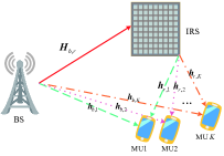
Figure 1: An IRS-aided communication system consisting of a base station (BS), multiple mobile users (MUs), and an IRS comprising many IRS units, where phase shifts incurred by the IRS units are remotely controlled by the BS.

We consider IRS-aided communications in the broadcast setting, where there are a BS with $M$ antennas and an IRS with $N$ IRS units, and $K$ single-antenna MUs, as shown in Fig. 1. We consider that the BS utilizes linear transmit precoding as the beamforming vector, denoted by $\bm{w}\in\mathbb{C}^{M\times 1}$, and thus the transmitted signal at the BS is $\bm{x}=\bm{w}{s}$ where ${s}$ is the broadcasted data. When BS broadcasts the signal $\bm{x}$, it will arrive at each MU via indirect and direct channels, and the received signal at each MU is the superposed signal from the two channels. More specifically, for the indirect channel, the transmitted signal $\bm{x}$ travels from the BS to the IRS, reflected by the IRS, and finally travels from the IRS to these $K$ MUs. For the direct channel, the transmitted signal $\bm{x}$ travels from BS to these $K$ MUs directly.

Let $\bm{\Phi}=\text{diag}(\beta_{1}e^{j\theta_{1}},\ldots,\beta_{N}e^{j\theta_{N}})$ denote the reflection coefficient matrix at the IRS, where $\beta_{n}$ and $\theta_{n}$ denote the amplitude factor and phase shift respectively. In this paper, we assume that the IRS only changes the phase of the reflected signal, i.e., $\theta_{n}\in[0,2\pi)$ and $\beta_{n}=1$. Let $\bm{H}_{\text{b},\text{r}}\in\mathbb{C}^{N\times M}$, $\bm{h}_{\text{r},i}^{H}\in\mathbb{C}^{1\times N}$, and $\bm{h}_{\text{b},i}^{H}\in\mathbb{C}^{1\times M}$ be the BS-IRS channel, IRS-$i^{th}$ MU channel, and BS-$i^{th}$ MU channel respectively. Then, the received signal at MU $i$ is given by

$${y_{i}}=(\bm{h}_{\text{r},i}^{H}\bm{\Phi}{\bm{H}_{\text{b},\text{r}}}+\bm{h}_{\text{b},i}^{H})\bm{w}{s}+{n_{i}},\ \ i=1,\ldots,K,$$ (1)

where ${n_{i}}\sim\mathcal{C}\mathcal{N}(0,\sigma^{2}_{i})$ denotes the additive white Gaussian noise at MU $i$.

We assume that the broadcasted data ${s}$ is normalized to unit power. Then, the signal-to-interference-plus-noise ratio (SINR) at MU $i$ can be written as

$$\text{SINR}_{i}=\frac{|\bm{h}^{H}_{i}(\bm{\Phi})\bm{w}|^{2}}{\sigma^{2}_{i}},$$ (2)

where $\bm{h}_{i}^{H}(\bm{\Phi})=\bm{h}^{H}_{\text{r},i}\bm{\Phi}\bm{H}_{\text{b},\text{r}}+\bm{h}^{H}_{\text{b},i}$ means the overall downlink channel from the BS to MU $i$.

II-B Problem definition

The problem of power control under QoS for broadcasting, is to minimize the transmitted power at the BS under QoS. Note that the transmitted power at the BS is $\|\bm{w}\|^{2}$, and that the QoS of MU $i$ is usually characterized by its SINR. Then, this problem can be formulated as

$$\text{(P1):~{}}\min_{\bm{w},\bm{\Phi}}~{} \|\bm{w}\|^{2}$$ (3a)

$$~{}\mathrm{s.t.}~{} \frac{|\bm{h}^{H}_{i}(\bm{\Phi})\bm{w}|^{2}}{\sigma^{2}_{i}}\geq\gamma_{i},~{}\forall i==1,\ldots,K,$$ (3b)

$$0\leq{\theta_{n}}<2\pi,\ n=1,\ldots,N,$$ (3c)

where $\gamma_{i}$ is the SINR target. Furthermore, without loss of generality, we assume that all MUs have the same SINR target and the same noise variance, i.e., $\gamma_{k}=\gamma,\sigma_{k}^{2}=\sigma^{2}$.

III Alternating optimization algorithm

In this section, we utilize alternating optimization, which is used for multivariate optimization in an alternating manner, to solve Problem (P1), as described in Algorithm 1. More specifically, we first optimize $\bm{w}$ given $\bm{\Phi}$, and then optimize $\bm{\Phi}$ given $\bm{w}$, which is performed iteratively to obtain the desired $\bm{w}$ and $\bm{\Phi}$. In the following, we describe the details of the $j^{th}$ iteration to illustrate the alternating optimization algorithm.

Optimizing $\bm{w}$ given $\bm{\Phi}^{(j-1)}$. Given $\bm{\Phi}^{(j-1)}$ obtained during the $(j-1)^{th}$ iteration, Problem (P1) becomes the conventional power control problem under QoS in the downlink broadcast channel without an IRS.

$$\text{(P2):~{}}\min_{\bm{w}}~{} \|\bm{w}\|^{2}$$ (4a)

$$~{}\mathrm{s.t.}~{} \frac{|\bm{h}^{H}_{i}(\bm{\Phi}^{(j-1)})\bm{w}|^{2}}{\sigma^{2}}\geq\gamma,~{}i=1,\ldots,K,$$ (4b)

Note that Problem (P2) is non-convex because of the non-convex constraint, which can be solved by a relaxation of Problem (P2) based on semi-definite programming (SDP) [16],

$$\text{(P3):~{}}\min_{\bm{X}}~{}~{}~{} \text{trace}(\bm{X})$$ (5a)

$$~{}\mathrm{s.t.}~{} \leavevmode\resizebox{305.33788pt}{}{$\text{trace}(\bm{X}\bm{H}_{i}(\bm{\Phi}^{j-1}))\geq\gamma\sigma^{2},~{}i=1,\ldots,K$},$$ (5b)

$$\bm{\bm{X}}\succeq 0,$$ (5c)

where $\bm{X}$ and $\bm{H}_{i}(\bm{\Phi}^{(j-1)})$ are defined as $\bm{X}:=\bm{w}\bm{w}^{H}$ and $\bm{H}_{i}(\bm{\Phi}^{(j-1)}):=\bm{h}_{i}(\bm{\Phi}^{(j-1)})\bm{h}_{i}(\bm{\Phi}^{(j-1)})^{H}$ respectively.

Apparently, Problem (P3) is an SDP, and we can utilize the convex optimization solvers (e.g., CVX [17]) to solve this problem. After $\bm{X}$ is available, the Gaussian randomization [18] is applied to obtain solution to Problem (P2). Note that, when utilizing the Gaussian randomization, we can obtain many candidate solutions to Problem (P2), and we select the one with the minimum power as the value of $\bm{w}$ during the $j^{th}$ iteration, denoted by $\bm{w}^{(j)}$.

Finding $\bm{\Phi}$ given $\bm{w}^{(j)}$. Given $\bm{w}^{(j)}$, Problem (P1) becomes the following feasibility check problem of finding $\bm{\Phi}$:

Algorithm 1 Alternating optimization to find $\bm{w}$ and $\bm{\Phi}$ for Problem (P1).

1:  Initialize $\bm{\Phi}$ as $\bm{\Phi}^{(0)}:=\text{diag}(e^{j\theta_{1}^{(0)}},\ldots,e^{j\theta_{N}^{(0)}})$, where $\theta_{n}^{(0)}$ $(n=1,2,\ldots,N)$ is chosen uniformly at random from $[0,2\pi)$;

2:  Initialize the iteration number $j\leftarrow 1$;

3:  while 1 do

3:      {Comment: Optimizing $\bm{w}$ given $\bm{\Phi}$:}

4:     Given $\bm{\Phi}$ as $\bm{\Phi}^{(j-1)}$, solve Problem (P3) to obtain $\bm{w}^{(j)}$;

5:     Compute the object function value $P_{t}^{(j)}\leftarrow\|\bm{w}^{(j)}\|^{2}$;

6:     if $1-\frac{P_{t}^{(j)}}{P_{t}^{(j-1)}}\leq\varepsilon$ then

7:        break; {Comment: $\varepsilon$ controls the number of executed iterations before termination. The algorithm terminates if the relative difference between the transmit power obtained during the $j^{th}$ iteration and the $(j-1)^{th}$ iteration is no greater than $\varepsilon$.}

8:     end if

8:      {Comment: Finding $\bm{\Phi}$ given $\bm{w}$:}

9:     Given $\bm{w}$ as $\bm{w}^{(j)}$, solve Problem (P6) to obtain $\bm{\Phi}^{(j)}$;

10:     if Problem (P6) is infeasible then

11:        break;

12:     end if

13:  end while

$$\text{(P4)}:\text{Find}~{}~{}~{} \bm{\Phi}$$ (6a)

$$\mathrm{s.t.}~{}~{}~{}~{}~{} \frac{|\bm{h}^{H}_{i}(\bm{\Phi})\bm{w}^{(j)}|^{2}}{\sigma^{2}}\geq\gamma,$$ (6b)

$$0\leq{\theta_{n}}<2\pi,\ n=1,...,N.$$ (6c)

Let $\bm{\phi}=[e^{j\theta_{1}},\ldots,e^{j\theta_{N}}]^{H}$, $\bm{a}_{i}=\text{diag}(\bm{h}^{H}_{\text{r},i})\bm{H}_{\text{b},\text{r}}\bm{w}^{(j)}$, and $b_{i}=\bm{h}^{H}_{\text{b},i}\bm{w}^{(j)}.$ Then, the (P4) can be rewritten as

$$\text{(P5)}:\text{Find}~{}~{}~{} \bm{\phi}$$ (7a)

$$\mathrm{s.t.}~{}~{}~{}~{}~{} \begin{bmatrix}\bm{\phi}^{H},~{}1\end{bmatrix}\bm{A}_{i}\begin{bmatrix}\bm{\phi}\\ 1\end{bmatrix}+{b}_{i}{b}_{i}^{H}\geq\gamma\sigma^{2}.$$ (7b)

$$|{\phi}_{n}|=1,\ n=1,\ldots,N.$$ (7c)

where $\bm{A}_{i}=\begin{bmatrix}\bm{a}_{i}\bm{a}_{i}^{H},&\bm{a}_{i}{b}_{i}^{H}\\ {b}_{i}\bm{a}_{i}^{H},&0\end{bmatrix}.$

Note that, since the constraints (7c) are non-convex, Problem (P5) is a non-convex optimization problem. However, by introducing an auxiliary variable $t$ satisfying $|t|=1$, Problem (P5) can be converted to a homogeneous quadratically constrained quadratic program (QCQP). Specifically, define

$$\bm{v}:=t\begin{bmatrix}\bm{\phi}\\ 1\end{bmatrix}=\begin{bmatrix}\bm{\phi}t\\ t\end{bmatrix},\text{and}\ \ \bm{V}:=\bm{v}\bm{v}^{H}.$$ (8)

Then, a relaxation of Problem (P5) based on SDP is

$$\text{(P6)}:\max_{\bm{V},\bm{\alpha}}\sum\nolimits_{i=1}^{K} \alpha_{i}$$ (9a)

$$\mathrm{s.t.}~{}~{}~{}~{}~{} \text{trace}(\bm{A}_{i}\bm{V})+{b}_{i}{b}_{i}^{H}\geq\alpha_{i}+\gamma\sigma^{2},$$ (9b)

$$\bm{V}_{n,n}=1,\ \ n=1,\ldots,N+1$$ (9c)

$$\bm{V}\succeq 0,\ \alpha_{i}\geq 0,i=1,\ldots,K,$$ (9d)

where variable $\alpha_{i}$ can be described as MU $i$’s “SINR residual” in the phase shift optimization [6].

Similar to Problem (P2), we can utilize the convex optimization solvers to solve problem (P6). After $\bm{V}$ is available, the Gaussian randomization is applied to obtain many candidate solutions to (P4), denoted by $[\bm{\Phi}^{(j)}_{1},\ldots,\bm{\Phi}^{(j)}_{c}]$ where $c$ is the number of candidate solutions. The rule of selecting one as the value of $\bm{\Phi}$ during the $j^{th}$ iteration, denoted by $\bm{\Phi}^{{(j)}}$, is described as follows.

First, we define

$$f:={\min({{|\bm{h}_{1}^{H}(\bm{\Phi})\overline{\bm{w}}|^{2}},\ldots,{|\bm{h}_{K}^{H}(\bm{\Phi})\overline{\bm{w}}|^{2}}})},$$ (10)

where $\overline{\bm{w}}=\frac{\bm{w}}{\|\bm{w}\|}$ denotes the transmit beamforming direction at the BS. Replacing $\bm{\Phi}$ and $\overline{\bm{w}}$ in Eq. (10) with $\bm{\Phi}^{(j-1)}$ and $\overline{\bm{w}}^{(j)}=\frac{\bm{w}^{(j)}}{\|\bm{w}^{(j)}\|}$ respectively, we can obtain the value of $f$ after optimizing $\bm{w}$ given $\bm{\Phi}^{(j-1)}$, denoted by $f^{(j)}_{\text{o}\bm{w}}$ (the subscript “o” represents optimization).

Next, after replacing $\bm{\Phi}$ and $\bm{w}$ in Eq. (10) with $\bm{\Phi}^{(j)}_{k}$ ($k=1,\ldots,c$) and $\bm{w}^{(j)}$ respectively, we can obtain the value of $f$ corresponding to $\bm{\Phi}^{(j)}_{k}$, denoted by $f^{(j)}_{k}$. If $f^{(j)}_{k}$ satisfies $f^{(j)}_{k}\geq f^{(j)}_{\text{o}\bm{w}}$, we incorporate it into a set $G$, and select the $\bm{\Phi}$ corresponding to the maximum element in $G$ as $\bm{\Phi}^{(j)}$. We denote the maximum element in $G$ as $f^{(j)}_{\text{o}\bm{\Phi}}$, which is the value of $f$ after optimizing $\bm{\Phi}$ given $\bm{w}^{(j)}$.

Proposition 1.

The rule of selecting one as the value of $\bm{\Phi}$ during the $j^{th}$ iteration, ensures the objective value in Problem (P2) is non-increasing over the iterations.

Proof: Let $P_{t}=\|\bm{\bm{w}}\|^{2}$ denote the transmit power. Given $\bm{\Phi}$, Problem (P2) can be rewritten as

$$\min_{\bm{w}}P_{t}$$ (11)

$$\mathrm{s.t.}\quad\frac{{P_{t}|\bm{h}_{i}^{H}(\bm{\Phi})\overline{\bm{w}}|}^{2}}{{\sigma}^{2}}\geq\gamma\quad\forall i\in\{1,2,\ldots,K\}.$$

Apparently, the minimum value of $P_{t}$ is

$$P_{t}=\frac{\gamma\sigma^{2}}{\min({|\bm{h}_{1}^{H}(\bm{\Phi})\overline{\bm{w}}|^{2}},\ldots,{|\bm{h}_{K}^{H}(\bm{\Phi})\overline{\bm{w}}|^{2}})}=\frac{\gamma\sigma^{2}}{f}.$$ (12)

Note that, if the value of $f$ after optimizing $\bm{w}$ given $\bm{\Phi}$ is non-decreasing over the iterations, then $P_{t}$ is non-increasing over the iterations; i.e., if $f^{(j+1)}_{\text{o}\bm{w}}\geq f^{(j)}_{\text{o}\bm{w}}$, then we have $P_{t}^{(j+1)}\leq P_{t}^{(j)}$. Based on the rule of selecting one as the value of $\bm{\Phi}$ during the $j^{th}$ iteration, it is easily to derive $f^{{(j)}}_{\text{o}\bm{\Phi}}\geq f^{(j)}_{\text{o}\bm{w}}$. Then, if the $\bm{w}^{(j+1)}$ is the optimal solution to Problem (P2) during the $(j+1)^{th}$ iteration, we derive $f^{(j+1)}_{\text{o}\bm{w}}\geq f^{{(j)}}_{\text{o}\bm{\Phi}}\geq f^{(j)}_{\text{o}\bm{w}}$. Hence, we have $P_{t}^{(j+1)}\leq P^{(j)}_{t}$, which means that $P_{t}$ is non-increasing over the iterations. $\square$

IV A lower bound for minimum transmit power

In this section, for the IRS-aided broadcast pattern, we derive a lower bound of the minimum transmit power.

We assume that the BS-MUs and IRS-MUs channel are Rayleigh fading, and that BS-IRS channel is LoS. We consider the uncorrelated Rayleigh fading channel model for IRS-$i^{th}$MU and BS-$i^{th}$MU; i.e. $\bm{h}_{r,i}\sim\text{ }\mathcal{C}\mathcal{N}(0,{\beta_{r,i}^{2}}{\bm{I}})$, $\bm{h}_{b,i}\sim\text{ }\mathcal{C}\mathcal{N}(0,{\beta_{b,i}^{2}}{\bm{I}})$, where $\beta_{r,i}^{2}$ and $\beta_{b,i}^{2}$ account for the path loss of IRS-MUs and BS-MUs respectively. Let ($x_{\text{BS}}$, $y_{\text{BS}}$, $z_{\text{BS}}$) and ($x_{\text{IRS}}$, $y_{\text{IRS}}$, $z_{\text{IRS}}$) be the coordinate of BS and IRS respectively. Then, the channel between the BS and IRS is given by [10]

$$\bm{H}_{b,r}=\sqrt{\frac{{\beta_{h}}^{2}}{{2}}}\bm{s}\bm{g}^{T},$$ (13)

where

$$\begin{array}[]{l}\bm{s}={[{s_{1}},\ldots,{s_{m}},\ldots,{s_{M}}]^{T}},\bm{b}=[{g_{1}},\ldots,{g_{n}},\ldots,{g_{N}}]^{T}\\ {s_{m}}=\exp\left({j\frac{{2\pi}}{\lambda}{d_{{\rm{BS}}}}(m-1)\text{sin}{\phi_{Lo{S_{1}}}}\text{sin}{\theta_{Lo{S_{1}}}}}\right),{\rm{}}m=1,\ldots,M\\ {g_{n}}=\exp\left({j\frac{{2\pi}}{\lambda}{d_{{\rm{IRS}}}}(n-1)\text{sin}{\phi_{Lo{S_{2}}}}\text{sin}{\theta_{Lo{S_{2}}}}}\right),{\rm{}}n=1,\ldots,N\\ {\theta_{Lo{S_{1}}}}={\tan^{-1}}\left({\dfrac{{{d_{{\rm{BS-IRS}}}}}}{{{z_{{\rm{IRS}}}}-{z_{{\rm{BS}}}}}}}\right),{\rm{}}{\theta_{Lo{S_{2}}}}=\pi-{\theta_{Lo{S_{1}}}}\\ {\phi_{Lo{S_{1}}}}=\pi-{\tan^{-1}}\left({\dfrac{{{y_{{\rm{IRS}}}}-{y_{{\rm{BS}}}}}}{{{x_{{\rm{IRS}}}}-{x_{{\rm{BS}}}}}}}\right),{\rm{}}{\phi_{Lo{S_{2}}}}=\pi+{\phi_{Lo{S_{1}}}},\end{array}$$ (14)

where $\lambda$ is wavelength, $d_{\text{BS}}$ and $d_{\text{IRS}}$ are the inter-antenna separation at the BS and IRS respectively, ${\phi_{Lo{S_{1}}}}$ and ${\phi_{Lo{S_{2}}}}$ are the LoS azimuth at BS and IRS respectively, ${\theta_{Lo{S_{1}}}}$ and ${\theta_{Lo{S_{2}}}}$ denote the elevation angle of departure at BS and elevation angle of arrival at IRS respectively, $\beta_{h}^{2}$ accounts for the path loss of IRS-BS, and $d_{\text{BS-IRS}}$ represent the distance between the BS and IRS.

Next, we present the details of deriving the lower bound of transmit power $P_{t}$ with respect to the number of IRS units $N$, the number of MUs $K$, and the number of antennas $M$, considering the following two cases of parameter settings: 1) $K=1$ and $M>1$; 2) $K>1$ and $M>1$. In addition, when discussing the case of $K=1$, we omit the subscript $i$ of $\beta_{b,i}$ and $\beta_{r,i}$ for presentation simplicity.

Case 1): $K=1$ and $M>1$. Based on Eq. (11), given $\bm{\Phi}$, the minimum transmit power $P_{t}$ is $P_{t}=\dfrac{{\sigma}^{2}\gamma}{|\bm{h}_{1}^{H}(\bm{\Phi})\overline{\bm{w}}|^{2}}$. Furthermore, because $\bm{h}_{1}^{H}(\bm{\Phi})$ is random variance, transmit power $P_{t}$ should be considered to be the average transmit power, which is more accurately written as

$$P_{t}=\frac{{\sigma}^{2}\gamma}{\mathbb{E}(|\bm{h}_{1}^{H}(\bm{\Phi})\overline{\bm{w}}|^{2})}.$$ (15)

This means that minimizing the transmit power is equivalent to maximizing the term $\mathbb{E}({|\bm{h}_{1}^{H}(\bm{\Phi})\overline{\bm{w}}|^{2}})$.

For $|\bm{h_{1}}^{\text{H}}(\bm{\Phi})\overline{\bm{w}}|$, we have

$$|\bm{h}_{1}^{H}(\bm{\Phi})\overline{\bm{w}}| =|\bm{h}_{r,1}^{{H}}{\bm{\Phi}}{\bm{H}_{b,r}}\overline{\bm{w}}+\bm{h}_{b,1}^{{H}}\overline{\bm{w}}|$$ (16)

$$\mathop{\leq}\limits^{(a)}|\bm{h}_{r,1}^{{H}}{\bm{\Phi}}{\bm{H}_{b,r}}\overline{\bm{w}}|+|\bm{h}_{b,1}^{{H}}\overline{\bm{w}}|.$$

Based on the triangle inequality, Eq. 16(a) holds if and only if $\arg(\bm{h}_{r,1}^{{H}}{\bm{\Phi}}{\bm{H}_{b,r}}\overline{\bm{w}})=\arg(\bm{h}_{b,1}^{{H}}\overline{\bm{w}})=\varphi_{0}$.

Let ${A}=|\bm{h_{r,1}}^{{H}}{\bm{\Phi}}{\bm{H}_{b,r}}\overline{\bm{w}}|,{B}=|h_{b,1}^{{H}}\overline{\bm{w}}|$. Then, the maximum value of $\mathbb{E}(|\bm{h}_{1}^{H}(\bm{\Phi})\overline{\bm{w}}|^{2})$ with respect to $\bm{\Phi}$ and $\overline{\bm{w}}$, denoted by $Q_{1}$, is given by

$$Q_{1} =\text{max}(\mathbb{E}(|{\bm{h}_{1}}^{H}(\bm{\Phi})\overline{\bm{w}}|^{2}))=\mathbb{E}(({A}+{B})^{2})$$ (17)

$$=\mathbb{E}({A}^{2})+2E({AB})+E({B}^{2}).$$

Next, we discuss how to derive each term in Eq. (17).

For $\mathbb{E}({A}^{2})$, we have

$$\left\{\begin{aligned} \mathbb{E}(A)&\mathop{=}\limits^{(a)}\mathbb{E}({\sum\nolimits_{n=1}^{N}}{|h_{r,1,n}^{H}}||{{\sum\nolimits_{m=1}^{M}}{{H}_{b,r,m,n}}\overline{w_{m}}|})\\ &=\mathbb{E}({\sum\nolimits_{n=1}^{N}}{|h_{r,1,n}^{H}}||C_{n}|)\\ &\mathop{=}\limits^{(b)}\mathbb{E}({|h_{r,1,1}^{H}}|)(|C_{1}|+|C_{2}|+\ldots+|C_{N}|),\\ \mathbb{E}^{2}(A)&=(|C_{1}|+|C_{2}|+\ldots+|C_{N}|)^{2}\mathbb{E}^{2}({|h_{r,1,1}^{H}}|)\\ &\mathop{=}\limits^{(c)}(N|C_{1}|)^{2}\frac{\beta_{r}^{2}\pi}{4}\mathop{\leq}\limits^{(d)}\frac{\pi N^{2}\beta_{h}^{2}\beta_{r}^{2}M}{8},\\ \textup{Var}(A)&=\textup{Var}({\sum\nolimits_{n=1}^{N}}|h_{r,1,n}^{H}||C_{n}|)\mathop{\leq}\limits^{(e)}\frac{\beta_{r}^{2}}{2}(2-\frac{\pi}{2})\times\frac{\beta_{h}^{2}M}{2}\times N,\\ \mathbb{E}(A^{2})&=\leavevmode\resizebox{389.89749pt}{}{$\mathbb{E}^{2}(\bm{A})+\textup{Var}(A)\leq\frac{\pi N^{2}\beta_{h}^{2}\beta_{r}^{2}M}{8}+\frac{N\beta_{r}^{2}\beta_{h}^{2}M}{4}(2-\frac{\pi}{2})$},\end{aligned}\right.$$ (18)

where $C_{n}={{\sum_{m=1}^{M}}{\bm{H}_{b,r,m,n}}\overline{w_{m}}}$, step (a) follows from the fact that $\arg(\bm{h_{r,1}}^{{H}}{\bm{\Phi}}{\bm{H}_{b,r}}\overline{\bm{w}})=\varphi_{0}$, step (b) follows from the fact that $\bm{h_{r,1}}\sim\text{ }\mathcal{C}\mathcal{N}(0,{\beta_{r,1}^{2}}{\bm{I}})$. For step (c), Since the element in ${\bm{H}_{b,r,m,n}}$ has the same amplitude and $[\overline{w_{1}},\ldots,\overline{w_{M}}]$ is the normalized vector, it is easy to derive that $|C_{1}|=\ldots=|C_{N}|$.  Step (c)  also follows from the fact that $|{h_{r,1,1}}^{H}|$ has distribution of Rayleigh with mean $\frac{\beta_{r}{\sqrt{\pi}}}{2}$, and steps (d)(e) follow from the fact that term $|C_{1}|^{2}\leq\frac{{M}\beta_{h}^{2}}{2}$ and that $|{h_{r,1,1}}^{H}|$ has distribution of Rayleigh with variance $\frac{\beta_{r}^{2}}{2}(2-\frac{\pi}{2})$.

For $\mathbb{E}({B}^{2})$, we have

$$\left\{\begin{aligned} \mathbb{E}({B})&\mathop{=}\limits^{(a)}\leavevmode\resizebox{375.80542pt}{}{$\mathbb{E}(\sum\nolimits_{m=1}^{M}|{h_{b,m}}^{H}\overline{w_{m}}|)=\mathbb{E}(\sum\nolimits_{m=1}^{M}|{h_{b,m}}^{H}||\overline{w_{m}}|)$}\\ &=(|\overline{w_{1}}|+|\overline{w_{2}}|+\ldots+|\overline{w_{M}}|)\mathbb{E}(|h_{b,1}^{{H}}|),\\ \mathbb{E}^{2}(B)&=(|\overline{w_{1}}|+|\overline{w_{2}}|+\ldots+|\overline{w_{M}}|)^{2}\mathbb{E}^{2}(|h_{b,1}^{{H}}|)\\ &\mathop{\leq}\limits^{(b)}(M|\overline{w_{1}}|)^{2}\frac{\beta_{b}^{2}\pi}{4}=\frac{\pi\beta_{b}^{2}M}{4},\\ \textup{Var}(B)&=\textup{Var}(\sum\nolimits_{m=1}^{M}|{h_{b,m}}^{H}||\overline{w_{m}}|)\mathop{\leq}\limits^{(c)}\frac{\beta_{b}^{2}}{2}(2-\frac{\pi}{2}),\\ \mathbb{E}(B^{2})&=\mathbb{E}^{2}(B)+\textup{Var}(B)\leq\frac{\pi\beta_{b}^{2}M}{4}+\frac{\beta_{b}^{2}}{2}(2-\frac{\pi}{2}),\end{aligned}\right.$$ (19)

where step (a) follows from the fact that $\arg(\bm{h}_{b,1}^{{H}}\overline{\bm{w}})=\varphi_{0}$, steps (b) and (c) follow from the fact that $|{h_{b,1}}^{H}|$ has distribution of Rayleigh with mean $\frac{\beta_{b}{\sqrt{\pi}}}{2}$ and variance $\frac{\beta_{b}^{2}}{2}(2-\frac{\pi}{2})$, step (b) also follows from the fact that term $(|\overline{w_{1}}|+|\overline{w_{2}}|+\ldots+|\overline{w_{M}}|)^{2}$ takes the maximum value if $|\overline{w_{1}}|=|\overline{w_{2}}|=\ldots=|\overline{w_{M}}|$ because of $\sum\nolimits_{m=1}^{M}|\overline{w_{m}}|^{2}=1$.

For $\mathbb{E}(AB)$, we have

$$\mathbb{E}(AB)=\sqrt{\mathbb{E}^{2}(A)\mathbb{E}^{2}(B)}=\frac{N\pi\beta_{r}\beta_{h}\beta_{b}M}{4\sqrt{2}}.$$ (20)

Substituting Eq. (18)-Eq. (20) into Eq. (17), we have

$$Q_{1} =\mathbb{E}({A}^{2})+2E({AB})+E({B}^{2})$$ (21)

$$=\frac{\pi N^{2}\beta_{b}^{2}\beta_{r}^{2}M}{8}+\frac{N\beta_{r}^{2}\beta_{h}^{2}M}{4}(2-\frac{\pi}{2})+\frac{N\pi\beta_{r}\beta_{h}\beta_{b}M}{2\sqrt{2}}$$

$$+\frac{\beta_{b}^{2}}{2}(2-\frac{\pi}{2})+\frac{\pi\beta_{b}^{2}M}{4}.$$

Then, substituting Eq. (21) into Eq. (15), the lower bound of the minimum transmit power at the BS in the case of $K=1,M>1$ is obtained in Eq. (22).

Case 2): $K>1$ and $M>1$. The minimum value of $P_{t}$ satisfying the constrains in Eq. (11), is

$$P_{t}=\frac{\gamma\sigma^{2}}{\min({\mathbb{E}({|\bm{h_{1}}^{H}(\bm{\Phi})\overline{\bm{w}}|^{2}})},\ldots,{\mathbb{E}({|\bm{h_{K}}^{H}(\bm{\Phi})\overline{\bm{w}}|^{2}})})}.$$ (23)

Based on ${\min({\mathbb{E}({|\bm{h_{1}}^{H}(\bm{\Phi})\overline{\bm{w}}|^{2}})},\ldots,{\mathbb{E}({|\bm{h_{K}}^{H}(\bm{\Phi})\overline{\bm{w}}|^{2}})})}\leq{\min({Q_{1},Q_{2},\ldots,Q_{K}})}$, the lower bound of the minimum transmit power at the BS is given by

$$P_{t}\geq P_{K>1,M>1}^{L}=\frac{r\sigma^{2}}{\min({Q_{1},Q_{2},\ldots,Q_{K}})},$$ (24)

where $Q_{i}=\max({\mathbb{E}(|\bm{h_{i}}^{H}(\bm{\Phi})\overline{\bm{w}}|^{2}}))$. Eq. (21) only presents how to get the value of $Q_{1}$, and we can use the same way to compute the other values of $Q_{i}$ ($i=1,\ldots,K$).

In addition, since Problem P(3) has $K$ linear constrains and $M^{2}$ variables, the complexity of solving Problem P(3) is ${O}((K+M^{2})^{3.5})$ for one iteration  [19]. Similarly, the complexity of solving Problem P(6) is ${O}(2K+(N+1)^{2})^{3.5})$ for one iteration. Hence, the complexity of the proposed alternating optimization is $O((K+M^{2})^{3.5})$+${O}(2K+(N+1)^{2})^{3.5})$ for one iteration. A future direction for us is to reduce the computational complexity and one potential idea is to use manifold optimization  [20].

V Simulation results

In this section, we utilize numerical results to validate the derived lower bound of the transmit power and the alternating optimization algorithm. We assume that the BS with uniform linear array of antennas is located at (0,0,0), and that the IRS with uniform linear array of IRS units is located at (0,50,0). The inter-antenna and inter-unit separation at BS and IRS are half wavelength. The purpose of deploying IRS is to improve the signal strength. To illustrate this benefiting, we assume that the MUs are uniformly located at the half circle centered at the IRS with radius 2 m as shown in Fig. 2, which are the cell-edge MUs. The channel models for BS-IRS, BS-MUs and IRS-MUs are the same as we described in Section IV, and the path loss is $\beta^{2}_{a,b}=C_{0}(d_{a,b}/D_{0})^{-\alpha}$, where $C_{0}=1$ m, $D_{0}=-30$dB, $d_{a,b}$ denotes the distance between $a$ and $b$, $\alpha$ is the path loss exponent. We set $\sigma^{2}=-30$ dBm, $\gamma=1dB$, and $\varepsilon=10^{-4}$. For BS-IRS, IRS-MUs, and BS-MUs, we set $\alpha=2,2.8,3.5$ respectively. In addition, we employ the conventional power control (i.e., without IRS, termed Without-IRS in the result figures) and power control with random phrase shift at the IRS (termed Random-IRS in the result figures) as our baselines.

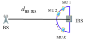
Figure 2: The location of IRS, BS and MUs in the simulation.

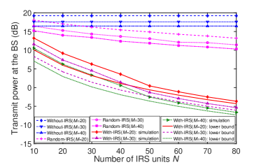
Figure 3: Transmit power vs. the number of IRS units ($K=1$).

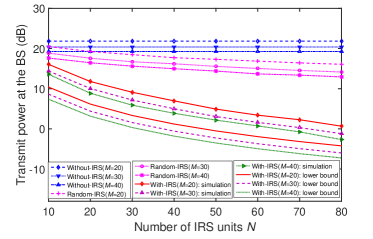
Figure 4: Transmit power vs. the number of IRS units ($K=2$).

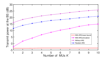
Figure 5: Transmit power vs. the number of MUs.

Figs. 3 and 4 show the variance of transmit power at BS with the number of IRS units for $M=20,30,40$ and $K=2$ respectively. We can see that, the transmit power decreases with the increase of the number of IRS units and the number of antennas at the BS, which significantly lower than the baselines. This indicates that, deploying IRS can actually improve the signal strength and thus decrease the transmit power at the BS. Furthermore, the results from Figs. 3 and 4 also show that the transmit power at the BS approaches the lower bound with the increase of the the number of IRS units, which coincide with the analysis results. Notice that Fig. 3 is more obvious than Fig. 4, and actually the speed of approaching the lower bound in Fig. 4 is extremely slow.

Fig.5 show the variance of transmit power at BS with the number of MUs $K$ ranging from 1 to 10 for $M=40,N=50$. The results show that, with the increase of the number of MUs, the transmit power increases, dramatically lower than the baselines, and the gap between the transmit power and the lower bound widens up. To obtaining a better bound which grows with $K$ is our future direction.

VI Conclusion

In this paper, we have proposed a solution to the power control under QoS for an IRS-aided wireless network. Specifically, we utilize the alternating optimization algorithm to jointly optimize the transmit beamforming at the BS and the passive IRS units at the IRS. Furthermore, we derived a lower bound of the minimum transmit power for the IRS-enhanced physical layer broadcasting. Simulation results show that, the transmit power at the BS approaches the lower bound with the number of IRS units, and is significantly lower than that of the communication system without IRS.

References

• [1] S. Zhang, Q. Wu, S. Xu, and G. Y. Li, “Fundamental green tradeoffs: Progresses, challenges, and impacts on 5G networks,” IEEE Communications Surveys Tutorials, vol. 19, no. 1, pp. 33–56, Firstquarter 2017.
• [2] S. Buzzi, C. I, T. E. Klein, H. V. Poor, C. Yang, and A. Zappone, “A survey of energy-efficient techniques for 5G networks and challenges ahead,” IEEE Journal on Selected Areas in Communications, vol. 34, no. 4, pp. 697–709, April 2016.
• [3] S. Hu, F. Rusek, and O. Edfors, “Beyond massive MIMO: The potential of data transmission with large intelligent surfaces,” IEEE Transactions on Signal Processing, vol. 66, no. 10, pp. 2746–2758, May 2018.
• [4] M. Di Renzo, M. Debbah, D.-T. Phan-Huy, A. Zappone, M.-S. Alouini, C. Yuen, V. Sciancalepore, G. C. Alexandropoulos, J. Hoydis, H. Gacanin, J. de Rosny, A. Bounceu, G. Lerosey, and M. Fink, “Smart radio environments empowered by AI reconfigurable meta-surfaces: An idea whose time has come,” arXiv preprint arXiv:1903.08925, 2019.
• [5] E. Basar, M. Wen, R. Mesleh, M. Di Renzo, Y. Xiao, and H. Haas, “Index modulation techniques for next-generation wireless networks,” IEEE Access, vol. 5, pp. 16 693–16 746, 2017.
• [6] Q. Wu and R. Zhang, “Intelligent reflecting surface enhanced wireless network via joint active and passive beamforming,” IEEE Transactions on Wireless Communications, 2019. [Online]. Available: https://doi.org/10.1109/TWC.2019.2936025
• [7] ——, “Beamforming optimization for intelligent reflecting surface with discrete phase shifts,” in IEEE International Conference on Acoustics, Speech and Signal Processing (ICASSP), May 2019, pp. 7830–7833.
• [8] “NTT DoCoMo and Metawave announce successful demonstration of 28GHz-band 5G using world’s first meta-structure technology,” https://www.marketwatch.com/press-release/ntt-docomo-and-metawave-announce-successful-demonstration-of-28ghz-band-5g-using-worlds-first-meta-structure-technology-2018-12-04, 28 October, 2019.
• [9] G. Zhou, C. Pan, H. Ren, K. Wang, W. Xu, and A. Nallanathan, “Intelligent reflecting surface aided multigroup multicast MISO communication systems,” arXiv preprint arXiv:1909.04606, 2019.
• [10] Q.-U.-A. Nadeem, A. Kammoun, A. Chaaban, M. Debbah, and M.-S. Alouini, “Asymptotic analysis of large intelligent surface assisted MIMO communication,” arXiv preprint arXiv:1903.08127, 2019.
• [11] Q. Wu and R. Zhang, “Intelligent reflecting surface enhanced wireless network: Joint active and passive beamforming design,” in IEEE Global Communications Conference (GLOBECOM), Dec 2018, pp. 1–6.
• [12] H. Guo, Y.-C. Liang, J. Chen, and E. G. Larsson, “Weighted sum-rate optimization for intelligent reflecting surface enhanced wireless networks,” arXiv preprint arXiv:1905.07920, 2019.
• [13] C. Pan, H. Ren, K. Wang, M. Elkashlan, A. Nallanathan, J. Wang, and L. Hanzo, “Intelligent reflecting surface aided MIMO broadcasting for simultaneous wireless information and power transfer,” arXiv preprint arXiv:1908.04863, 2019.
• [14] J. Zhao, “Optimizations with intelligent reflecting surfaces (IRSs) in 6G wireless networks: Power control, quality of service, max-min fair beamforming for unicast, broadcast, and multicast with multi-antenna mobile users and multiple IRSs,” arXiv preprint arXiv:1908.03965, 2019.
• [15] N. Sidiropoulos, T. Davidson, and Z.-Q. Luo, “Transmit beamforming for physical-layer multicasting,” IEEE Transactions on Signal Processing, vol. 54, no. 6, pp. 2239–2251, 2006.
• [16] H. Cramér, Random Variables and Probability Distributions.   Cambridge University Press, 2004.
• [17] M. Grant and S. Boyd. CVX: MATLAB software for disciplined convex programming. [Online]. Available: http:cvxr.com/cvx
• [18] A. M.-C. So, J. Zhang, and Y. Ye, “On approximating complex quadratic optimization problems via semidefinite programming relaxations,” Mathematical Programming, vol. 110, no. 1, pp. 93–110, 2007.
• [19] N. D. Sidiropoulos, T. N. Davidson, and Z.-Q. Luo, “Transmit beamforming for physical-layer multicasting,” IEEE Trans. Signal Process., vol. 54, no. 6, pp. 2239–2250, Jun. 2006.
• [20] C. Pan, H. Ren, K. Wang, W. Xu, M. Elkashlan, A. Nallanathan, and L. Hanzo, “Intelligent reflecting surface for multicell mimo communications,” arXiv preprint arXiv:1907.10864, 2019.